
Submitted:
02 August 2024
Posted:
02 August 2024
You are already at the latest version
Abstract
The effective baryon-baryon potential can be derived in the framework of quark model. The configurations with different quark spatial distributions are mixed naturally when two baryons are getting close. The effect of configuration mixing in chiral quark model (ChQM) is studied by calculating the effective potential between two nonstrange baryons in the channels I J = 01, 10 and 03. For comparison the results of color screening model (CSM) are also presented. Generally the configuration mixing will lower the potential when the separation between two baryons is small, and its effect will be ignorable when the separation becomes large. Due to the screened color confinement, the configuration mixing is rather large, which leads to stronger intermediate-range attraction in CSM. while the effect of configuration mixing is small in ChQM due to the quadratic confinement and σ-meson exchange, which is responsible for the intermediate-range attraction.
Keywords:
baryon-baryon interaction
; quark model
; configuration mixing
1. Introduction
The study of the dibaryon states have attracted great effort from both theorists and experimentalists since Jaffe’s prediction of the H particle [1]. The dibaryon is a color singlet multi-quark system with a sufficiently smaller size and is believed to be a prospective field to study the strong interaction phenomenology because the dibaryon may provide more information on quantum chromodynamics, the fundamental theory of strong interaction.
Baryon are well founded object. To bind two baryons together to form a dibaryon state is not a easy task, because too few states are discovered in experiments so far. Deuteron with isospin-spin-parity is a loosely bound state of proton and neutron, where the separation between two nucleons is rather large. with is believed to be a compact object of six quarks, which is reported by WASA@COSY collaboration [2]. The primary results of STAR@RHIC favors the existence of dibaryon state with [3]. With the advance of experiments, maybe more dibaryon states will be reported.
To bind two baryons, the attraction between two baryons are necessary. So the baryon-baryon effective potential is needed. Quark model is an effective approach to describe the properties of baryons, it is also applied to derive the baryon-baryon effective potentials [4,5,6,7,8,9,10,11,12,13,14,15,16,17,18]. In deriving the effective potential, generally quark cluster model is employed, in which the six quarks are grouped into two three-quark clusters and the internal motions of three-quark cluster are frozen. However, for the compact hexaquark system or if the two baryons are too close, it is reasonable to assume the quark delocalization, which is similar to the electron percolation in molecules. In 1990s, F. Wang and his collaborators developed a model-quark delocalization color screening model (QDCSM) [19] based on the Glashow-Isuger model. In QDCSM, the two new ingredients have been introduced. One is the quark delocalization, another is the color screening, taking into account the differences of confinement interaction inside a single baryon and between two color singlet baryon. The quark delocalization in QDCSM is a convenient way to realize a specific configuration mixing. The model can give a good description of nucleon-nucleon interactions, and a natural explanation of the similarity between molecular force and the nuclear force [19]. CSM is the QDCSM without quark delocalization.
By introducing the exchange of Goldstone bosons and their partner -meson between quarks, the Chiral quark model (ChQM) can also give a good description of nuclear force. So far, the configuration mixing is not considered in ChQM in calculating the baryon-baryon effective potential. In the present work, the effect of configuration mixing in ChQM is studied by calculating the baryon-baryon effective potentials. To simplify the calculation, we limit our calculation in the two flavor world, nonstrange system. The resonating group method (RGM) [20,21,22,23] is used to do the calculation. In molecular physics, the configuration interaction is a post-Hartree-Fock linear variational method for solving the non-relativistic Schrödinger equation within the Born-Oppenheimer approximation for a quantum chemical multi-electron system.
This paper is organized as follows. In section II, the model Hamiltonian and the symmetry bases are described. In Section III the calculation method is presented . The results are given in section IV and a conclusion is given in section V.
2. Quark Model and Wave Functions
2.1. The Chiral Quark Model
The Salamanca version of ChQM is chosen as a representative of chiral quark models [24,25]. It has been successfully applied to describe both hadron spectroscopy and nucleon-nucleon interactions. The model details can be found in Refs. [24,25]. The Hamiltonian in the baryon-baryon sector is
where () is the pion (sigma) mass, is the chiral coupling constant related to the coupling constant by , is a cutoff parameter, and is the Yukawa function defined as . is the kinetic energy of the center of mass. All other symbols have their usual meanings. The model parameters are fixed by the spectrum of baryons, and is fixed by fitting the scattering phase shifts. The fitted parameters are taken from Ref. [25] and given in Table 1. The absolute nucleon mass is controlled by a constant term in the confinement potential that does not affect the baryon-baryon interaction.
2.2. The Olor Screening Model
The Hamiltonian of the CSM is the same as that of ChQM with two modifications. First, there is no and meson exchange; second, the screened color confinement is used between quark pairs resident in different baryons. That is
2.3. Wave Functions
The symmetry bases of the wave functions for nonstrange six-quark system () can be constructed through the group chain such as
The symmetry basis for six quarks systems has the form
Where are the strong interaction conserved quantum numbers: isospin and spin. K denotes the intermediate quantum numbers, , which represent the symmetry of orbital, spin-isospin SU. is fixed due to the color singlet requirement. L and R are left and right gaussians, the single-particle orbital wave functions in the ordinary quark cluster model,
where is a reference center and b is a baryon size parameter. m and n are the numbers of quarks resident in left and right orbits, respectively. For some interesting sets of quantum numbers , the allowed intermediate quantum numbers K are listed in Table 2. Where take their maximum values, the eigenenergies are independent of . The twenty-seven bases for channel are shown in the Appendix A.
The spatial configurations of quarks are denoted by (). Configuration mixing means that different quark spatial distribution will mixed up. The eigen wave function is the linear combination of symmetry bases under the cluster approximation,
The numbers of the coupling channels for and are: 27, 27 and 10, respectively.
For different configurations, different orbital symmetries are allowed, the results are listed in Table 3.
3. Calculation Method
To study the baryon-baryon interaction, the Schrödinger equation for 6-quark system has to be solved,
where the eigen wave function is the linear combination of the symmetry bases under the cluster approximation, which has been given in the second section. By using Eq.(6), Eq.(7) becomes
where k stands for . The eigen energy of the system can be obtained by solving the generalized eigen equation. The calculation of the 6-body Hamiltonian matrix elements on the symmetry basis is performed by the well known fractional parentage expansion technique [21]. First the 6-body Hamiltonian with pairwise terms is reduced 2-body Hamiltonian, for example the Hamiltonian for the fifth and sixth particles, by making use the properties of identical particles. Second the symmetry basis is separated into two parts, 4-body (the first to the fourth particles) and 2-body (5th and 6th particles) using the coefficients of fractional parentage. Then the matrix element of 6-body Hamiltonian can be reduced to the product of coefficients of fractional parentage, 4-body overlaps and 2-body matrix elements.
where is the 4-body overlap. is the two body matrix element and represents the two-body operator for the last pair. and are the total coefficients of fractional parentage. All the needed coefficients can be obtained from the Chen’s book [26,27]. For the details, one can refer the Ref. [21]. As an example, a expression of the matrix element in the configuration of is given in Appendix B.
4. The Results and Discussions
The effective potentials between two baryons in the 2-flavor world are calculated in the framework of the chiral quark model and the quark delocalization color screening model with configuration mixing. The effective potential is defined as
where is the eigen-energy of 6-quark system with separation S between left and right gaussians. Here, we only give some results of non-strange 6-quark system with quantum numbers and the 03. In order to check the contribution of the configuration mixing to the effective potentials of the baryon-baryon system, we give the results of configuration only and that of all configuration mixing (denoted by ) in Figure 1, Figure 2 and Figure 3. One can see that the effects of configuration mixing on the effective potentials are different for two models, and the effects vary with the separation. Generally the configuration mixing will reduce the energy of the system compared with that of configuration only, and the effects decrease with the increase of the separation.
Figure 1 shows the effective N-N potential for channels with configuration comparing with the configuration mixing. It’s clear that the configuration only have an effective intermediate-range attraction, but it is a little weaker MeV than that of configuration mixing in ChQM. However in the CSM, the configuration mixing has a stronger effective attraction about 25 MeV than that of configuration only. One can also see that there is no intermediate-range attraction in CSM if the color screening effect is not taken into account ( fm). The configuration mixing lowers the energy of the system a little, but it is still no attraction. This infers that the quadratic confinement prevent the configuration mixing. Only when the confinement is screened, then the configuration mixing can be developed. The reason can be used to explain the small effects of configuration mixing in ChQM, where the confinement is not screened and the intermediate-range attraction is mainly provided by the -meson exchange. So it is sufficient to use baryonic structure () only when studying interaction in the ChQM. To see the contribution of different configurations to the energy of the system at each separation, the percentages of different configurations at given separation are calculated and are shown in Table 4. From the table, one can see that the baryonic structure ( configuration) is always the main configuration, it dominates when the separation becomes large in both model. In ChQM, the configuration dominates even the separation is small. The color confinement expels other configuration. It is a good approximation to consider only the configuration in ChQM. For CSM, the configuration mixing has important contribution to effective potential, there are considerable non- configurations in the state when the separation is small, fm. So it is necessary to consider configuration mixing in CSM.
Figure 2 shows the effective N-N potential for channels . The results are similar to that of (Figure 1). The percentages of different configurations at given separation are shown in Table 5. The similarity to Table 4 is also apparent.
Figure 3 illustrates the effective - potential for channels . The - are decuplet-decuplet channel, many theoretical calculations and some experiments state the existence of the -dibaryon named as [2,23,28,29,30]. In ChQM, it’s clear that the - with configuration only has an similar intermediate-range attraction about 150 MeV to that of configuration mixing. At small separation, stronger attraction is obtained with the configuration mixing. In CSM, when color screening is not considered ( fm), modest attractions are obtained in configuration only and configuration mixing calculations. When color screening is considered, fm, a very strong attraction MeV appear. The percentages of different configurations at given separation are shown in Table 6. In this case, the configuration is no longer the main component when the separation is small, a compact state is expected.
Comparing Figure 3 with the Figure 1 and Figure 2, one can see that there a deeper intermediate-range attraction between two ’s than that between two nucleons. This can be explained by the structure difference of N to . In resonance, the spins of quarks are all parallel, the color-spin interaction in one-gluon exchange potential gives a positive contribution to energy of the state, while the spins of quarks in nucleon are parallel or anti-parallel, half to half, the color-spin contribution to the energy is negative, so the mass of is larger than that of nucleon. Going to the two-baryon system, the contribution of color-spin interaction has more chances to be negative. In addition, the configuration mixing let quarks have larger space to move, which lower the kinetic energy of the system. In this way, systems generally have deeper attraction. From Table 6, one can see that the non- configurations are still considerable even the separation is large, fm.
5. Summary
By taking into account the configuration mixing in the framework of ChQM and CSM, we calculate the effective potentials of the system such as as well as the . It can be seen that configuration mixing will reduce the energy of the system, which leads to the stronger intermediate-range attraction in both models. Although the effect of configuration mixing is not important in ChQM, it is indispensable in CSM. If the compact six-quark state exists, the configuration mixing must be considered in the calculation of the binding energy of the system, even in ChQM, because the effect of configuration mixing is not small when the separation between two clusters is small. QDCSM is a simple version of CSM with configuration mixing, only the configuration is considered, but the left and right single particle wave function is delocalized ones, and . In this way, all the configurations are taken into account but with only one variational parameter . This approach is an economic way, greatly reduce the computational burden.
Author Contributions
Conceptualization, J. Ping; methodology, H. Huang and X. Zhu; investigation, X. Zhu; writing—original draft preparation, X. Zhu; writing—review and editing, H. Huang and J. Ping; funding acquisition, J. Ping. All authors have read and agreed to the published version of the manuscript.
Funding
This research was funded by National Natural Science Foundation of China under Contract Nos. 11675080, 11775118, 11535005 and 11865019.
Institutional Review Board Statement
Not applicable.
Data Availability Statement
Research data have been given in the manuscript.
Conflicts of Interest
The authors declare no conflicts of interest.
Appendix A. The 27 Symmetry Bases, for the State with α = (IJ) = (01)
Appendix B. The Matrix Element in the Configuration of L3 R3
where is the orbital matrix element, are color, isospin and spin matrix elements, respectively. For the operators, , , , we have the following results.
References
- Jaffe, R. L. Phys. Rev. Lett. 1977, 38, 195. [Google Scholar] [CrossRef]
- Bashkanov, M. [CELSIUS-WASA Collab.] Phys. Rev. Lett. 2009, 102, 052301.
- Adam, J. et al. [STAR Collab.] Phys. Lett. B 2019, 790, 490. [Google Scholar] [CrossRef]
- Machleidt, R.; Holinde, K.; Elster, Ch. Phys. Rep. 1987, 149, 1. [Google Scholar] [CrossRef]
- Nagels, M. M.; Rijken, T. A.; de Swart, J. J. Ann. Phys. 1973, 79, 338. [Google Scholar]
- Nagels, M. M.; Rijken, T. A.; de Swart, J. J. Phys. Rev. D 1975, 12, 744; 1977, 15, 2547.
- Cottingham W., N. et al. Phys. Rev. D 1973, 8, 800. [Google Scholar]
- Maessen, P. M. M.; Rijken, T. A.; de Swart, J. J. Phys. Rev. C 1989, 40, 2226. [Google Scholar]
- Holzenkamp, B.; Holinde, K.; Speth, J. Nucl. Phys. A 1989, 500, 485. [Google Scholar]
- Oka, M.; Shimizu, K.; Yazaki, K. Nucl. Phys. A 1987, 464, 700. [Google Scholar]
- Koike, Y.; Shimizu, K. Yazaki, K. Nucl. Phys. A 1990, 513, 653. [Google Scholar] [CrossRef]
- Shimizu, K. Rep. Prog. Phys. 1989, 52, 1. [Google Scholar] [CrossRef]
- Yazaki, K. Properties and interactions of hyperons, ed. B. F. Gibson et al, World Scientific, Singapore, 1994, p.189.
- Straub, U.; Zhang, Z. Y.; Bräuer, K.; Faessler, A.; Khadkikar, S. H.; Lübeck, G. Nucl. Phys. A 1988, 483, 686. [Google Scholar]
- Straub, U. et al Phys. Lett. B 1988, 200, 241. [Google Scholar] [CrossRef]
- Fujiwara, Y.; Nakamoto, C.; Suzuki, Y. Phys. Rev. Lett. 1996, 76, 2242. [Google Scholar] [CrossRef] [PubMed]
- Fujiwara, Y.; Nakamoto, C.; Suzuki, Y. Prog. Theor. Phys. 1995, 94, 215; 94, 353.
- Nakamoto, C.; Suzuki, Y.; Fujiwara, Y. Prog. Theor. Phys. 1995, 94, 65. [Google Scholar] [CrossRef]
- Wang, F.; Wu, G. H.; Teng, L. J. Goldman, T. Phys. Rev. Lett. 1992, 69, 2901. [Google Scholar] [CrossRef] [PubMed]
- Ping, J. L.; Wang, F.; Goldman, T. Nucl. Phys. A 1999, 657, 95. [Google Scholar]
- Wang, F.; Ping, J. L.; Goldman, T. Phys. Rev. A 1995, 51, 1648. [Google Scholar]
- Valcarce, A.; Garcilazo, H. et al. Rep. prog. Phys. 2005, 2005 68, 965. [Google Scholar] [CrossRef]
- Ping, J. L.; Huang, H. X.; Pang, H. R.; Wang, F.; Wong, C. W. Phys. Rev. C 2009, 79, 024001. [Google Scholar]
- Valcarce, A.; Gonzalez, P.; Garcilazo, H.; Fernandez, F.; Vento, V. Phys. Lett. B 1996, 367, 35. [Google Scholar] [CrossRef]
- Entem, D. R.; Fernández, F.; Valcarce, A. Phys. Rev. C 2000, 62, 034002. [Google Scholar]
- Chen, J. Q. Tables of the Clebsh-Gordan, Racah and Subduction Coefficients of SU(n) Groups, World Scientific, Singapore, 1987.
- Chen, J. Q. Tables of the SU(mn)⊃SU(m)×SU(n) Coefficients of Fractional Parentage, World Scientific, Singapore. 1991. n.
- Bashkanova, M.; Brodsky, S. Phys. lett. B 2013, 727, 438. [Google Scholar]
- Ping, J. L.; Wang, F.; Goldman, T. Nucl. Phys. A 2001, 688, 871. [Google Scholar]
- Valcarce, A.; Garcilazo, H.; Fernandez, F.; Gonzalez, P. Rep. Prog. Phys. 2005, 68, 965 and references there in.
- Chen, L. Z.; Pang, H. R.; Huang, H. X.; Ping, J. L.; Wang, F. Phys. Rev. C 2007, 76, 014001. [Google Scholar]
Figure 1.
Effective potential (in MeV) vs. baryon-baryon separation (in fm) for N-N () channels.
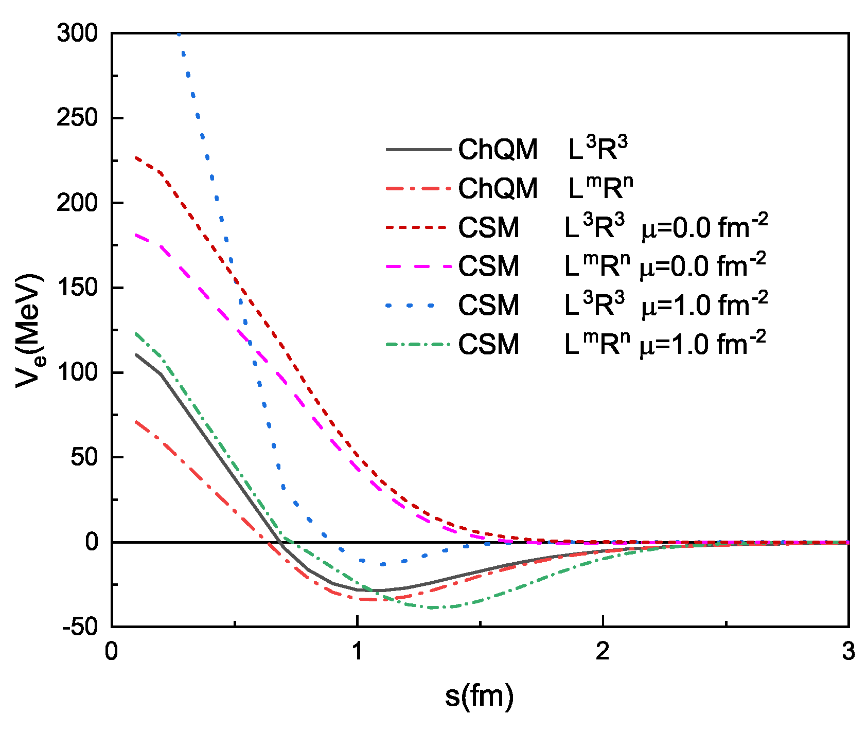
Figure 2.
Effective potential (in MeV) vs. baryon-baryon separation (in fm) for N-N () channels.
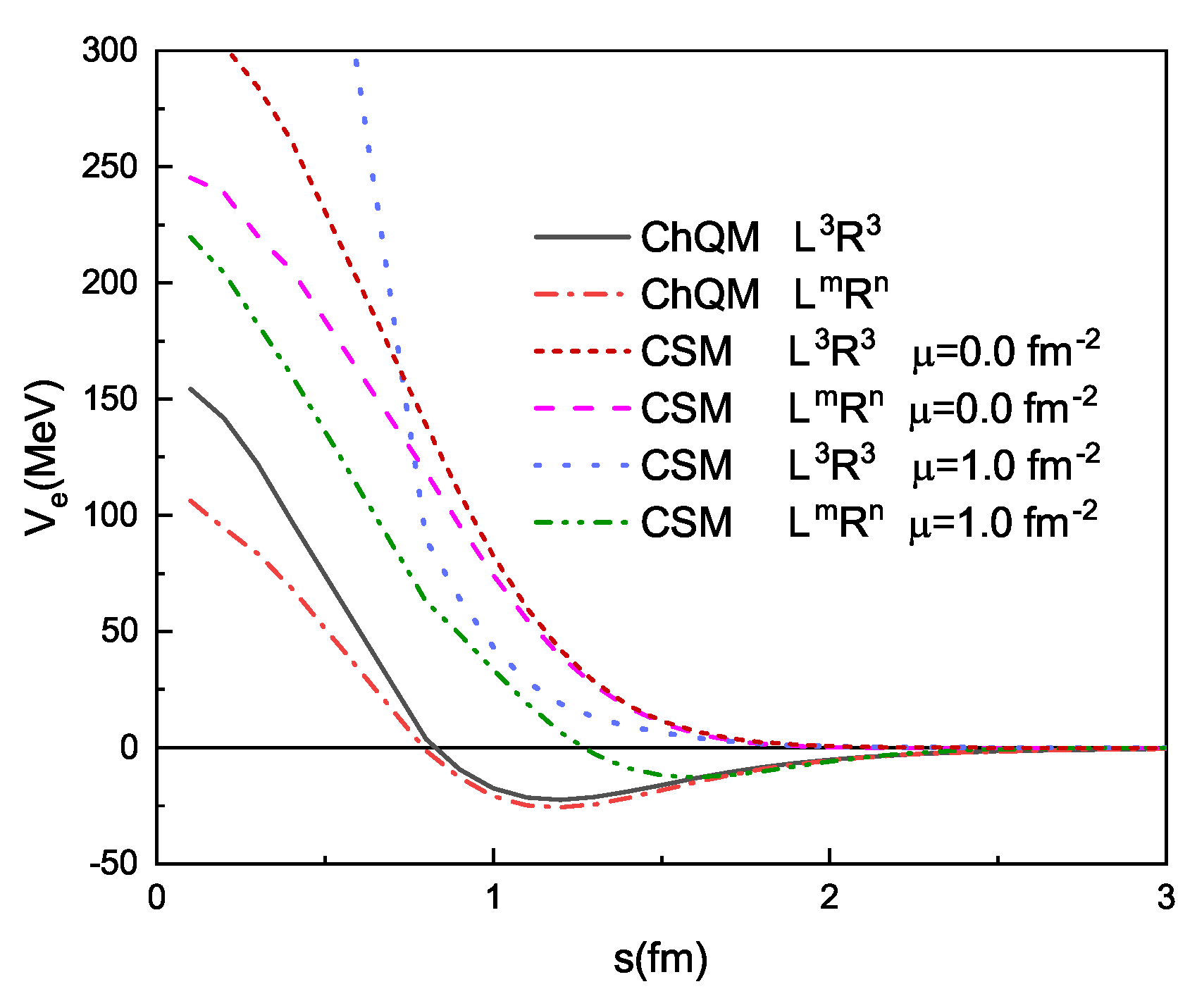
Figure 3.
Effective potential (in MeV) vs. baryon-baryon separation (in fm) for - () channels.
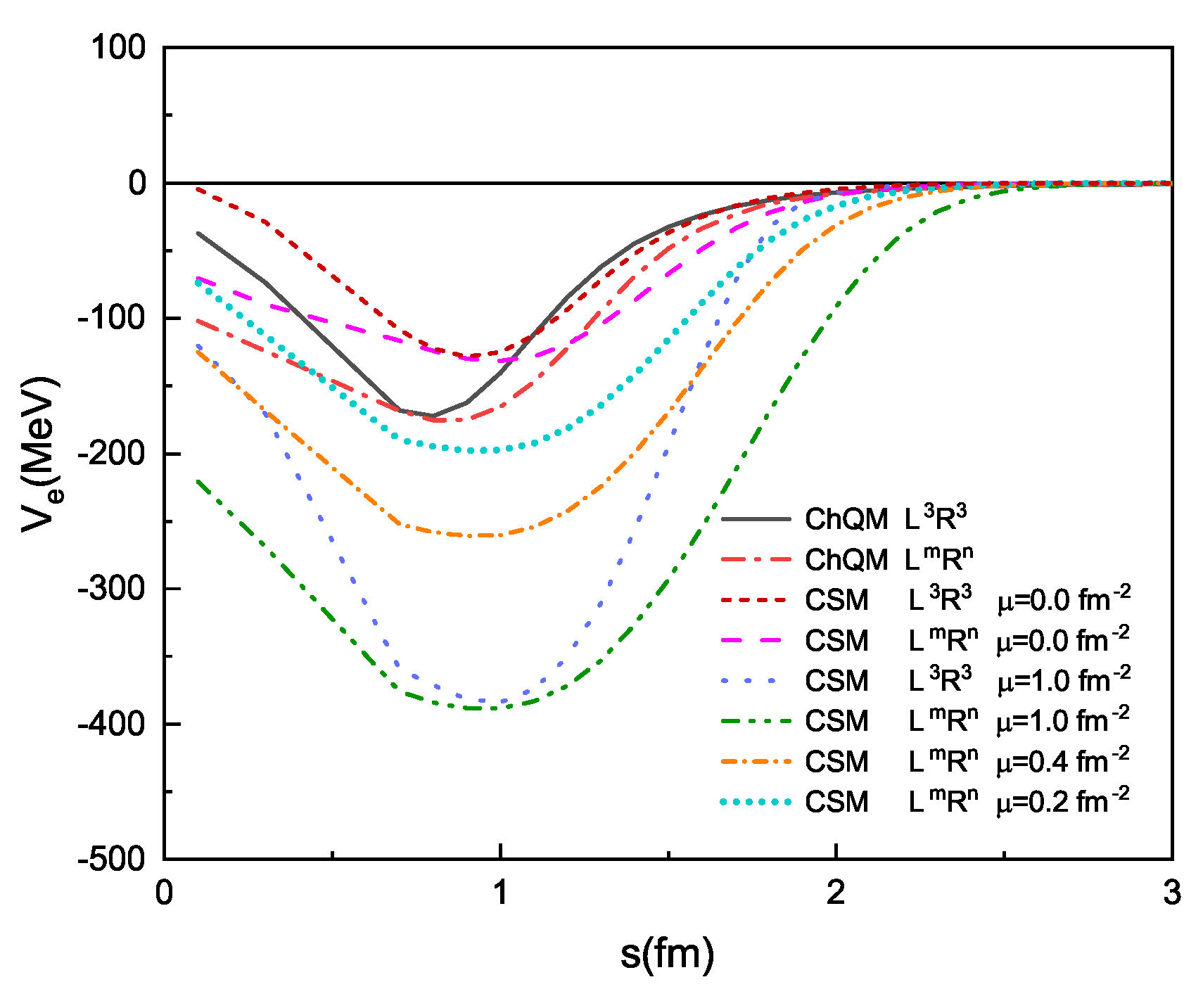

Table 1.
Model parameters.
| Model | ChQM | CSM | |
|---|---|---|---|
| Quarks | b (fm) | 0.518 | 0.603 |
| (MeV) | 313 | 313 | |
| (MeV) | 313 | 313 | |
| Confinements | (MeV·fm) | 46.938 | 25.13 |
| (fm) | − | ||
| (fm) | − | ||
| OGE | 0.485 | 1.54 | |
| Goldstone bosons | (MeV) | 675 | − |
| (MeV) | 138 | − | |
| (fm) | − |
Table 2.
The allowed for interesting sets of . The irreducible representation of is denoted by the partitions.
Table 2.
The allowed for interesting sets of . The irreducible representation of is denoted by the partitions.
| K | |||||||
|---|---|---|---|---|---|---|---|
| 01 | [6][44] | [51][321] | [42][51] | [42][33] | [42][2211] | [42][321] | [42][411] |
| 10 | [6][33] | [51][321] | [42][51] | [42][33] | [42][2211] | [42][321] | [42][411] |
| 03 | [6][33] | [42][33] | |||||
Table 3.
The allowed orbital symmetry for given configuration .
| [6] | 1 | 1 | 1 | 1 | 1 | 1 | 1 | |
| [51] | 0 | 1 | 1 | 1 | 1 | 1 | 0 | |
| [42] | 0 | 0 | 1 | 1 | 1 | 0 | 0 | |
| [33] | 0 | 0 | 0 | 1 | 0 | 0 | 0 |
Table 4.
The percentages of configurations in the states with and fm (CSM).
| fm | fm | fm | ||||
|---|---|---|---|---|---|---|
| ChQM | CSM | ChQM | CSM | ChQM | CSM | |
| 0.15 | 0.15 | 0.00 | 0.00 | 0.00 | 0.00 | |
| 0.00 | 0.01 | 0.00 | 0.08 | 0.00 | 0.01 | |
| 0.13 | 0.19 | 0.17 | 0.03 | 0.01 | 0.12 | |
| 0.44 | 0.30 | 0.66 | 0.78 | 0.78 | 0.74 | |
| 0.13 | 0.19 | 0.17 | 0.03 | 0.01 | 0.12 | |
| 0.00 | 0.01 | 0.00 | 0.08 | 0.00 | 0.01 | |
| 0.15 | 0.15 | 0.00 | 0.00 | 0.00 | 0.00 | |
| fm | fm | fm | ||||
| ChQM | CSM | ChQM | CSM | ChQM | CSM | |
| 0.00 | 0.00 | 0.00 | 0.00 | 0.00 | 0.00 | |
| 0.00 | 0.00 | 0.00 | 0.00 | 0.00 | 0.00 | |
| 0.00 | 0.09 | 0.00 | 0.00 | 0.00 | 0.00 | |
| 1.00 | 0.82 | 1.00 | 1.00 | 1.00 | 1.00 | |
| 0.00 | 0.09 | 0.00 | 0.00 | 0.00 | 0.00 | |
| 0.00 | 0.00 | 0.00 | 0.00 | 0.00 | 0.00 | |
| 0.00 | 0.00 | 0.00 | 0.00 | 0.00 | 0.00 | |
Table 5.
The percentages of configurations in the states with and fm (CSM).
| fm | fm | fm | ||||
|---|---|---|---|---|---|---|
| ChQM | CSM | ChQM | CSM | ChQM | CSM | |
| 0.13 | 0.07 | 0.00 | 0.00 | 0.00 | 0.00 | |
| 0.00 | 0.00 | 0.01 | 0.01 | 0.00 | 0.00 | |
| 0.14 | 0.15 | 0.18 | 0.22 | 0.00 | 0.04 | |
| 0.46 | 0.56 | 0.63 | 0.54 | 1.00 | 0.92 | |
| 0.14 | 0.15 | 0.18 | 0.22 | 0.00 | 0.04 | |
| 0.00 | 0.00 | 0.01 | 0.01 | 0.00 | 0.00 | |
| 0.13 | 0.07 | 0.00 | 0.00 | 0.00 | 0.00 | |
| fm | fm | fm | ||||
| ChQM | CSM | ChQM | CSM | ChQM | CSM | |
| 0.00 | 0.00 | 0.00 | 0.00 | 0.00 | 0.00 | |
| 0.00 | 0.00 | 0.00 | 0.00 | 0.00 | 0.00 | |
| 0.00 | 0.04 | 0.00 | 0.00 | 0.00 | 0.00 | |
| 1.00 | 1.00 | 1.00 | 1.00 | 1.00 | 1.00 | |
| 0.00 | 0.04 | 0.00 | 0.00 | 0.00 | 0.00 | |
| 0.00 | 0.00 | 0.00 | 0.00 | 0.00 | 0.00 | |
| 0.00 | 0.00 | 0.00 | 0.00 | 0.00 | 0.00 | |
Table 6.
The percentages of configurations in the states with and fm (CSM).
| fm | fm | fm | ||||
|---|---|---|---|---|---|---|
| ChQM | CSM | ChQM | CSM | ChQM | CSM | |
| 0.29 | 0.15 | 0.00 | 0.00 | 0.00 | 0.00 | |
| 0.00 | 0.01 | 0.02 | 0.03 | 0.00 | 0.01 | |
| 0.11 | 0.19 | 0.05 | 0.08 | 0.05 | 0.11 | |
| 0.20 | 0.30 | 0.86 | 0.78 | 0.90 | 0.76 | |
| 0.11 | 0.19 | 0.05 | 0.08 | 0.05 | 0.11 | |
| 0.00 | 0.01 | 0.02 | 0.03 | 0.00 | 0.01 | |
| 0.29 | 0.15 | 0.00 | 0.00 | 0.00 | 0.00 | |
| fm | fm | fm | ||||
| ChQM | CSM | ChQM | CSM | ChQM | CSM | |
| 0.00 | 0.07 | 0.00 | 0.03 | 0.00 | 0.00 | |
| 0.00 | 0.01 | 0.00 | 0.00 | 0.00 | 0.00 | |
| 0.00 | 0.04 | 0.00 | 0.00 | 0.00 | 0.00 | |
| 1.00 | 0.76 | 1.00 | 0.94 | 1.00 | 1.00 | |
| 0.00 | 0.04 | 0.00 | 0.00 | 0.00 | 0.00 | |
| 0.00 | 0.01 | 0.00 | 0.00 | 0.00 | 0.00 | |
| 0.00 | 0.07 | 0.00 | 0.03 | 0.00 | 0.00 | |
Disclaimer/Publisher’s Note: The statements, opinions and data contained in all publications are solely those of the individual author(s) and contributor(s) and not of MDPI and/or the editor(s). MDPI and/or the editor(s) disclaim responsibility for any injury to people or property resulting from any ideas, methods, instructions or products referred to in the content. |
© 2024 by the authors. Licensee MDPI, Basel, Switzerland. This article is an open access article distributed under the terms and conditions of the Creative Commons Attribution (CC BY) license (https://creativecommons.org/licenses/by/4.0/).
Copyright: This open access article is published under a Creative Commons CC BY 4.0 license, which permit the free download, distribution, and reuse, provided that the author and preprint are cited in any reuse.


