
Submitted:
02 August 2024
Posted:
02 August 2024
You are already at the latest version
Abstract
The dominant part of energy performance of a building consists of consumption of heating and lighting. Both heating and lighting systems of buildings work at their designed efficiency for most of the buildings’ lifetimes. Interference with existing systems is costly considering replacements and construction adjustments. Therefore, considerable effort must be put into the design of these systems during the building design phase. The article is focused on luminaire layout design strategy, which affects the number of luminaires in a building and therefore their power consumption and the sustainability of the building. A genetic algorithm with radiosity implemented has been used to find suitable placements of luminaires of a single type in a model room to decrease the number of luminaires as much as possible. Three outcomes of optimal luminaire layout design are presented in this paper, including design strategy conclusions. Results of calculation outcomes are verified by software DIALux, that is commonly used for designing lighting systems.
Keywords:
lighting design
; genetic algorithm
; luminaire layout design
; luminous intensity curve
1. Introduction
While designing lighting systems for indoor working places, a designer must take several requirements into account. As far as illumination [1], visual comfort [2], and performance of occupancy [3] is considered, it can be said in general that the illumination levels provided by the lighting system (artificial lighting, daylighting) must be suitable for the activities for which the indoor space is intended [4]. This and more are taken into account by the European Standard EN 12464-1 [5] mandatory on the territory of the European Union.
The initial phase of lighting design for a specific environment prioritizes the establishment of illuminance requirements. This adheres to European Standards [5] and is achieved by calculating the required luminous flux and the corresponding number of luminaires. Lighting software facilitates an initial, uniform grid-based layout of these luminaires, each possessing identical luminous flux, photometric distribution curve, and mounting height.
However, a skilled lighting designer transcends this preliminary analysis. To achieve a comfortable environment, additional factors are integrated into the design process. These encompass:
- Spatial distribution of luminance: This ensures a balanced illumination scheme, surpassing a uniform application of illuminance.
- Light directionality: Strategic manipulation of light direction influences mood and accentuates specific spatial features.
- Color Rendering Index (CRI): A high CRI guarantees accurate and natural color perception within the environment [Error! Reference source not found.].
- Chromatic response of materials: The interaction of light with various materials necessitates consideration to optimize the overall visual experience.
- Architectural characteristics: The spatial dimensions, configuration, and intended purpose of the environment all play a crucial role in shaping the final lighting design.
By incorporating these scientific principles, lighting designers create environments that are not only functional but also aesthetically compelling.
The simplest, and most commonly used, electric lighting system for commercial spaces is consisting of luminaires only of a single type laid out in a regular symmetric pattern on the ceiling using recessed, surface-mounted, or pendant luminaires. Such design can be obtained by using various professional lighting design software and its wizard feature for indoor spaces. Another way would be to use professional lighting design software for manual irregular luminaire placement where the compliance with the standard can be checked by calculating the luminous flux distribution in the chosen indoor space. Finding manually the optimal luminaire layout design can be difficult and its impact on lighting power density [6] is uncertain.
Research on lighting optimization so far leverages advanced computational techniques, notably neural networks, competition over resource algorithm, evolutionary algorithms and genetic algorithms, to enhance the efficiency and quality of lighting systems in various environments.
Neural network technique was applied in 2013 by Wang et al. [7] to map the relationship among dimming levels of luminaires grid without optimizing the luminaire layout pattern. In 2017, in addition to dimming, Mendez [8] took into account the total cost of lighting optimization using the competition over resource algorithm [9].
In 2019, Mandal et al. [10] applied particle swarm optimization, an evolutionary algorithm [11], with three decision variables (regular luminaire spacing along the length and width and luminaire mounting height) to find the optimal grid-based pattern of luminaires. The number of luminaires was determined by a loop in the program, which makes the algorithm inefficient. Grid-based luminaire layout design based on particle swarm optimization was verified with DIALux software [12] simulation in 2022 by Ji-Qing Qu et al. [13].
Luminaire layout design is more often solved using genetic algorithms. In 2015, Mattoni et al. [14] used a single-objective genetic algorithm to optimize indoor luminaire layout design by considering energy efficiency, Uo, and UGR with two variable luminaires in uniform grid-based pattern. In 2016, Madias et al. [15] proposed a multi-objective nondominated sorting genetic algorithm [16] to optimize the two objectives of reducing the energy consumption of buildings by dimming of one type of luminaire and improving the Uo of uniform grid-based luminaire pattern. In 2022, Watini et al. [17] applied genetic algorithms for economical optimization of school room lighting by optimizing spacing in a grid-based luminaire pattern.
Another option of luminaire layout design is to use of a non-grid-based luminaire pattern. Such design was proposed in 2017 by Plebe et al. [18] with more flexible approach to the interior lighting design by considering , Uo, and energy consumption, but only with general omnidirectional light source.
Genetic algorithms were also used for lighting optimization of outdoor lighting [19], plant lighting [20] and street lighting [21].
In this paper, we propose a method to obtain the most optimal luminaire layout design by running a genetic algorithm script based on real luminaires and independent of the conventional grid-based luminaire pattern. The goal is to meet the requirements of technical standards while reducing the number of luminaires needed, and consequently, to increase lighting installation sustainability. Another benefit of the proposed method could be the architecturally interesting unconventional non-grid luminaire layout design. In this paper, only artificial lighting is considered.
2. Model Room
A cuboid shaped test model room has been chosen to be used for luminous flux distribution calculations for the defined luminaire layout of the chosen type. These calculations were carried out using DIALux software [12] and our own implementation of the global illuminating algorithm radiosity, requiring the room’s surfaces to reflect light diffusely. To acquire specific requirements for the lighting system of the model room from the mentioned standard, we chose a room used for handwriting, writing on typewriters, reading and processing of data according to reference number 34.2 [5]. There are several specific conditions required by the standard that have to be met by the designed lighting system:
- – maintained average illuminance of 500 lx;
- – illuminance uniformity 0.6;
- – unified glare rating RUG limit value 19;
- – colour rendering index (CRI) 80.
Beside walls, floor and ceiling of the model room, a reference plane has been used. In this specific case the reference plane represented work surfaces of the room, i.e., top surfaces of desks used in the room. Since placements of desks were ignored in this project, which is an approach often used in lighting system designs, the horizontal reference plane filled the whole model room 0.85 m above the floor as suggested in standard [5].
According to standard ČSN EN 36 0011-1 [22] the values of and should be measured in a grid on the reference plane starting 1 m away from walls with spacing from 0.5 m to 2 m between adjacent points. However, we used a denser grid (Figure 1b) to make the calculated values of and more precise. Also, this grid of calculation points is suggested by default by DIALux.
The model room will meet the stated average illuminance requirement if the reference plane’s average illuminance will not drop below this value over the course of operation of the lighting system. The initially needed average illuminance is calculated by using the maintenance factor MF [23]. MF indicates the depreciation of luminous flux emitted from luminaires and reflected from surfaces at the end of the maintenance period. To get initial illuminances, maintained illuminances need to be divided by maintenance factor . The value of MF has been set to 0.8 as suggested for very clean indoor spaces by DIALux. Lighting uniformity is the ratio of minimum maintained illuminance to of the reference plane and, as required, must be greater than the stated value.
The calculation of has not been implemented into our algorithm. Whether the output luminaire layout from the algorithm meets the requirement is instead validated by DIALux by using horizontal calculation areas filling the whole model room at the height of 1.2 m above the floor using calculation point spacing 10 cm with views towards the north, south, west, and east walls (Figure 1a).
is a parameter of light sources and luminaires that is dependent on their light spectrum, but independent on the model room and its luminaire placements and as such, it was therefore not included into the calculations. All the used luminaire types and their light sources met the minimum requirement.
The presented genetic algorithm was developed and tested using a model room of dimensions 10 m × 5 m × 4 m (Figure 1a). No barriers or equipment were considered. As generally assumed while designing lighting systems for indoor working places, the surfaces of the model room showed uniform diffuse reflections with reflectance ρ (ratio of reflected and incident light) of the following defined values:
- floor reflectance ;
- wall reflectance ;
- ceiling reflectance .
The rendering algorithm radiosity has been implemented to be used by the genetic algorithm for the objective function feedback, calculating the given luminaire layout design’s quality. As radiosity is an application of the finite element method, the model room’s surfaces had to be divided into smaller facets (rectangular facets of dimensions 0.2 m × 0.2 m have been used). These were used by our implemented radiosity method for special luminous flux distribution calculations including 6 reflections. The number of reflections has been limited to 6 after several radiosity test runs using only a single luminaire of type MSTR SLB 4×18W (exported from software BuildingDesign – Wils library [24]) placed in the model room in the center of the ceiling, for illuminances of the facets have been affected by less than 10 % using more than 6 reflections by the algorithm. The radiosity reflection test run results are graphically shown in Figure 2.
A rectangular grid of evenly spaced control points – used for illuminance calculations – was placed on the reference plane with 25 cm distances between neighboring points (Figure 1b). Luminaires were placed in the plane of the model room’s raster ceiling starting 0.5 m from the eastern and western wall and 0.4 m from the northern and southern wall as depicted in Figure 1a with available positions spaced 0.6 m apart. Three luminaire types were used in this project from manufacturer Trevos, i.e., TT LED, PSV PISA T8 OP and PSV PISE T8 PAR (Figure 3), all being designed for a 600 × 600 mm gypsum or raster ceiling. All placed luminaires were oriented identically with their planes C0°-C180° [25] parallel to the room’s y-axis as depicted in Figure 1a.
3. Genetic Algorithm
Genetic algorithms (GA) belong to the group of evolutionary algorithms. Similar to living organisms, solutions (individuals) are defined by their structure (genotype), representing the parameter coding, and by their parameter set (phenotype), representing behavior, response and features of the solutions. The structure is typically coded as a vector-termed string with elements being described as features [26]. Each solution is evaluated based on its parameter set and selected if the set fits the constraints and conditions of the examined environment or task. The ability to survive and reproduce in a specific environment is called fitness and the function evaluating fitness is called the objective function. The selection must maintain or increase the fitness of solution sets that are called populations. Each set of solutions corresponds to a so-called generation. Each generation starts from a selected set of parent individuals. Each following generation picks a set of parent individuals from the previous generation. Individuals of populations are created from their parents by their string recombination and mutation. The crossover mechanism combines the strings of the two parents. A modified one-point crossover was used in the presented solution described in section 3.2.
The mutation mechanism changes a one or several values of the string directly. The implementation of mutation depends on the character of the task, and it is therefore briefly described later. Both recombination and mutation are applied only with a certain probability. The probability of crossover is typically high (more than 90 %) in comparison to mutation, which must be low (under 10 %). High probability of mutation makes the optimization difficult because of the high rate of changes in the solutions’ strings.
GAs are capable of reaching the vicinity of optimal or suboptimal solutions. There are several reasons why outputs of GAs are rarely optimums. The main are random algorithm behavior and difficulties to overcome suboptimal solutions. Therefore, designer’s corrections are required after getting an output in order to get closer to the global or local optimum. A great advantage of GAs is that there is no need to describe the functional dependency of genotype on phenotype. While getting the resulting parameters from input strings is quite easy (for example by calculations or experiments), the opposite procedure is much more difficult or impossible due to several possible solutions or the complexity of the task. This is also visible in the presented paper, where getting illuminance and uniformity values from known luminaire positions is relatively easy to calculate, but evaluating luminaire positions from known illuminance and uniformity values is significantly more complex.
3.1. Grid of Possible Solutions
A grid of possible luminaire positions has been defined. Such grid actually represents raster ceilings widely used in office buildings. The grid respected also the size of the used luminaires meaning that they could never overlap.
Possible luminaire positions were numbered and ordered as a string. The presence of the luminaire at a given position was represented by a Boolean value 1 (True) and the absence was represented by a Boolean value 0 (False). This approach enabled the optimization of both the luminaire layout and the luminaire count.
3.2. Recombination
A simple one-point crossover based on random selection of a string splitting point can result in an offspring being completely different from its parents. Consider, for example, the extreme case where both parents are solutions with luminaires concentrated into opposite halves of the luminaire grid, i.e., the first parent’s string consists of ones the whole first half and of zeros the second half, the latter parent’s string consists of zeros the first half and of ones the second half. If the splitting point is then chosen to be the middle of the parents’ strings, one offspring solution will have only zeros in the string, the other only ones, i.e., one offspring solution will not contain any luminaires whatsoever, the other will contain luminaires in all possible positions. Both offspring solutions will not be similar even in terms of the resulting illuminance and uniformity compared to their parents. Even though the parents might fit the criteria for the model room’s lighting system, both their offspring solutions are unusable solutions.
In order to ensure, that such pathological behavior does not occur, one-point crossover has been modified in such a way that not the whole parts of parents’ strings were switched. Instead, luminaire positions following the crossover point up to a limit were switched to create the offspring strings. This way only a few luminaires at most are added or removed from the solution after the crossover has been applied as seen in Figure 4b. In Figure 4a luminaire positions are only switched.
As the outcome of the presented custom one-point crossover depends on the order of the two input solutions, two offspring solutions are created switching the order of the input parent solutions.
3.3. Mutation
As in crossover, a similar issue occurs in mutations. A simple inversion of an element of the solution’s string affects the luminaire count, i.e., a luminaire would be added or removed. Better results in terms of output solution convergence towards the optimum and time efficiency have been achieved by implementing a permutation that changes the luminaire layout only, i.e., luminaire count does not change, only string elements are switched. In the final form of the algorithm up to 3 permutations were allowed per solution and generation.
3.4. Objective Function
A simple objective function has been defined for solution optimization. In the case of our project, GA was minimizing the outcome of the following equations:
where:
- and are calculated values of average illuminance and lighting uniformity,
- and are calculated values of average illuminance and lighting uniformity,
- α is the preference factor,
- denotes the sum of used luminaries (sum of 1s in the string)
- is the population size
The objective function was set up to include and optimize the luminaire count, being a dominant factor. By doing so, solutions were evaluated from the point of view of power consumption, preferring solutions containing fewer luminaires if average illuminance and lighting uniformity requirements are still met.
The implemented preference factor α is a number between 0 and 1 that corresponds to the designer’s wish to prefer average illuminance over lighting uniformity or vice versa with the defined weight. Authors tried several settings of the factor but the results differed just slightly. Only values of α close to the bounds 0 or 1 had a significant influence on the outcome. The presented results were always optimized with a balanced preference, i.e., α was set to 0.5.
The raster ceiling design allowed that a limited number of positions of luminaires could be placed which enabled us to pre-calculate illuminance values of the reference plane in calculation points for single luminaires in all available positions. Calculating the reference plane illumination values for a lighting system design (multiple luminaires) is then simply achieved by summing up the pre-calculated illuminance values for the used luminaires. Since these calculations were used for each solution’s evaluation, the GA running time has been considerably shortened.
3.5. GA Settings
All settings of the used GA are summarized in Table. 1. Parents for the offspring solutions are chosen using tournament 1 of 4, i.e., from the whole generation 4 solutions are chosen and the one with the highest fitness picked. This procedure is done twice (two parents are needed) creating two offspring solutions using custom recombination (section 3.2) with a probability of 90 % as mentioned in Table 1. Furthermore, mutation is applied to both offspring solutions with a probability of 1 % followed by the permutation of one, two, or three element pairs of the solutions’ strings with probabilities defined in Table 1.
Elitism has been used in the final algorithm picking the best solution of a generation and preserving it in its original form for the following generation. Then another copy of this best solution is passed to the following generation undergoing mutation. This approach was supposed to improve the algorithm convergence, however, no noticeable advantages were observed.
4. Results and Analysis
Sample outputs of the implemented GA are presented in this section. The output solutions were always a little different for a given luminaire type after each run of the GA. This phenomenon was discussed above and is caused by the initial random string generation of the first generation as well as by random mutations, permutations, crossovers, and tournaments (section 3). The output solutions are always close to the optimum but almost never the exact optimum. The designer is always supposed to choose a suitable solution after multiple runs of GA and adjust the luminaire positions if needed.
Although the outputs using a given luminaire type were different, the basic patterns were always similar. Examples of GA outputs using luminaires TT LED, PSV PISA SDK T8 OP, and PSV PISA SDK T8 PAR are in Figure 5a, 5b, 5c, respectively, and Table 2. All results are presented in their raw form as they were generated by GA. Em and U0 values presented in Table 2 were confirmed and UGRL values calculated by recreating the GA outputs (luminaire placements) in software DIALux [12]. All presented GA outputs complied with the UGRL requirement across the whole calculation plane, i.e., there were no restrictions for an occupant to work at any desired place in the model room with view directions towards the north, south, west, or east wall.
As expected, the luminaire count was dependent on the output luminous flux of the given luminaire type and on its luminous intensity curve shape (Figure 3). Looking at Table 2 the total output luminous flux of all placed luminaires of type PSV PISA SDK T8 PAR was 37584 lm, while in case of luminaire type PSV PISA SDK T8 OP it was 47520 lm, making the first mentioned type more efficient for the chosen model room. Both luminaires use the same light source with slightly different luminaire light output ratios [27], but their luminous intensity curves are different as seen in Figure 3b and 3c. Looking further at the total power consumption of the used luminaire types, the solution using TT LED luminaires compared to PSV PISA SDK T8 OP luminaires require 3.5 times less electrical power for the lighting system to meet the set requirements.
4.1. Luminaire Placement Dependency on Luminous Intensity Curve Shape
The luminaire positions of the GA solutions are dependent on their luminous intensity curves. Luminaires with narrower luminous intensity curves, i.e., luminaires emitting luminous flux predominantly in the vertical direction, were placed close to the corners of the model room to ensure the required uniformity of the illuminated reference plane. This effect can be seen in case of luminaires TT LED and PSV PISA SDK T8 OP (Figure 5a and 5b). There are 4 luminaires in very similar positions near the corners in both cases. On the other hand, luminaires of type PSV PISA SDK T8 PAR have a wide luminous intensity curve in direction parallel to the model room’s y-axis which enables GA to place them closer to the x-axis (longitudinal) of the model room (Figure 5c).
Luminaires PSV PISA SDK T8 OP and PSV PISA SDK T8 PAR are fitted with exactly the same quantity of the same light sources. However, the resulting total count of placed luminaires in each run of GA differed in both cases needing at least 4 luminaires less for solutions using luminaires PSV PISA SDK T8 PAR (Table 2), even though in this case the total luminous flux of all placed luminaires was 20 % lower. It appears that the luminaire PSV PISA SDK T8 PAR is more appropriate for the chosen model room. By comparing the illuminance levels of the reference plane of both solutions it is evident that the illuminance pattern of the luminaire PSV PISA SDK T8 PAR solution is more spread to the sides of the model room along the x-axis which leads to a better uniformity value even though less luminaires are used (Figure 5c and 5b).
Luminous intensity curves of luminaire TT LED and PSV PISA SDK T8 OP are quite similar as it is obvious from Figure 3. Therefore, the resulting total flux of both solutions is also similar (within 10 %, see Table 2). Less total luminous flux is needed in the case of TT LED since its intensity curve is little bit more widened between angles ±30◦ and the requested uniformity is met with greater spacing of the luminaires compared to the PSV PISA SDK T8 OP output solution. The overall low count of TT LED luminaires is given by its higher nominal luminous flux higher for about 40 % than the nominal flux of the other presented luminaires.
5. Conclusion
An optimization method of luminaire placement was presented in this paper with a few sample results (see Figure 5 and Table 2). The optimization was based on a genetic algorithm. The presented method settings made it possible to place luminaires in a specified irregular luminaire pattern, which is the main difference from various previous research. The irregular luminaire pattern generated by genetic algorithm may be very attractive for architects, because the irregular pattern could be influenced by the configuration of the genetic algorithm to achieve different architectonic solutions.
By using our GA implementation, it is possible to generate single-luminaire-type placements for different luminaire types which can be compared and the most effective solution chosen. Some luminaires may fit specific room requirements more appropriately than other as it was shown in the output examples. Investment costs and power consumption can be very different even for designs using different luminaires with the same build-in light sources. Common computer design programs can generate rectangular grid-based luminaire patterns. Although this might be the preferred layout for most lighting systems due to its simplicity, it is very often inefficient in comparison to randomly placed luminaires, for example by genetic algorithm presented in this paper. The designed GA can also be configured to generate symmetrical solutions, which might be visually more preferable.
Author Contributions
Conceptualization, Z.P. and R.B.; methodology, M.B.; software, R.B.; validation, M.B., Z.P. and R.B.; formal analysis, R.B.; investigation, R.B.; resources, M.B.; data curation, R.B.; writing—original draft preparation, R.B.; writing—review and editing, Z.P.; visualization, Z.P.; supervision, M.B.; project administration, M.B.; funding acquisition, M.B. All authors have read and agreed to the published version of the manuscript.
Funding
This research was funded by Czech Technical University in Prague, grant number SGS23/167/OHK3/3T/13
Conflicts of Interest
The authors declare no conflicts of interest. The funders had no role in the design of the study; in the collection, analyses, or interpretation of data; in the writing of the manuscript; or in the decision to publish the results.
References
- Baniya, R.R.; Tetri, E.; Halonen, L. A study of preferred illuminance and correlated color temperature for LED office lighting. Light Eng. 2015, 23, 39. [Google Scholar]
- Hwang, T.; Kim, J.T. Effects of indoor lighting on occupants’ visual comfort and eye health in a green building. Indoor Built Environ. 2011, 20, 75–90. [Google Scholar] [CrossRef]
- Vanus, J.; Martinek, R.; Nedoma, J.; Fajkus, M.; Cvejn, D.; Valicek, P.; Novak, T. Utilization of the LMS Algorithm to Filter the Predicted Course by Means of Neural Networks for Monitoring the Occupancy of Rooms in an Intelligent Administrative Building. IFAC-PapersOnLine 2018, 51. [Google Scholar] [CrossRef]
- Van Duijnhoven, J.; Aarts, M.P.J.; Kort, H.S.M. Personal lighting conditions of office workers: An exploratory field study. Lighting Res. Technol. 2021, 53, 285–310. [Google Scholar] [CrossRef]
- EN 12464-1 Light and lighting - Lighting of work places: Part 1: Indoor work places. European Committee for Standardization (CEN). Brussels, Belgium, 2022.
- Montoya, F.G.; Peña-García, A.; Juaidi, A.; Manzano-Agugliaro, F. Indoor lighting techniques: An overview of evolution and new trends for energy saving. Energy Build. 2017, 140, 50–60. [Google Scholar] [CrossRef]
- Wang, Z.; Tan, Y.K. Illumination control of LED systems based on neural network model and energy optimization algorithm. Energy Build. 2013, 62, 514–521. [Google Scholar] [CrossRef]
- Mendes, L.A.; Freire, R.Z.; dos Santos Coelho, L.; Moraes, A.S. Minimizing computational cost and energy demand of building lighting systems: A real time experiment using a modified competition over resources algorithm. Energy Build. 2017, 139, 108–123. [Google Scholar] [CrossRef]
- Mohseni, S.; Gholami, R.; Zarei, N.; Zadeh, A.R. Competition over resources: a new optimization algorithm based on animals behavioral ecology. In Int. Conf. Intell. Netw. Collab. Syst., Salerno, Italy, 10-12 September 2014.
- Mandal, P.; Dey, D.; Roy, B. Optimization of luminaire layout to achieve a visually comfortable and energy-efficient indoor general lighting scheme by particle swarm optimization. Leukos. 2019, 17, 91–106. [Google Scholar] [CrossRef]
- Kennedy, J.; Eberhart, R. Particle swarm optimization. In Proceedings of the ICNN’95-International Conference on Neural Networks, Perth, WA, Australia, 27 November–1 December 1995; Volume 4, pp. 1942–1948. [Google Scholar]
- DIALux software. Available online: https://www.dialux.com/ (accessed on 24 July 2024).
- Ji-Qing, Q.; Qi-Lin, X.; Ke-Xue, S. Optimization of Indoor Luminaire Layout for General Lighting Scheme Using Improved Particle Swarm Optimization. Energies. 2022, 15, 1482. [Google Scholar]
- Mattoni, B.; Gori, P.; Bisegna, F. A step towards the optimization of the indoor luminous environment by genetic algorithms. Indoor Built Environ. 2015, 26, 590–607. [Google Scholar] [CrossRef]
- Madias, E.N.D.; Kontaxis, P.A.; Topalis, F.V. Application of multi-objective genetic algorithms to interior lighting optimization. Energy Build. 2016, 125, 66–74. [Google Scholar] [CrossRef]
- K. Deb; A. Pratap; S. Agarwal; T. Meyarivan A fast and elitist multi-objective genetic algorithm: NSGA-II. IEEE Trans. Evol. Comput. 2002, 6, 182–197. [Google Scholar] [CrossRef]
- Watini, U.; Yusuf, M.I.; Kurniato, R. Application of Genetic Algorithm for Economical Optimization of School Room Lighting According to SNI 03-6575-2001. Jurnal Teknik Elektro. 2022, 14, 60–66. [Google Scholar] [CrossRef]
- Plebe, A.; Pavone, M. Multi-objective Genetic Algorithm for Interior Lighting Design. In Proceedings of the International Workshop on Machine Learning, Optimization, and Big Data, Volterra, Italy, 14–17 September 2017; pp. 222–233. [Google Scholar]
- Corcione, M.; Fontana, L. Optimal Design if Outdoor Lighting Systems by Genetic Algorithms. Light res Technol. 2003, 35, 261–280. [Google Scholar] [CrossRef]
- Ferentinos, K.P.; Albright, L.D. Optimal Design of Plant Lighting System by Genetic Algorithms. Eng Appl Artif Intell 2005, 18, 473–484. [Google Scholar] [CrossRef]
- Shintabella, R.; Abdullah, A.G.; Hakim, D.L. Application of Genetic Algorithm in Optimizing Redesign of Street Lighting, In: The 5th Annual Applies Science and Engineering Conference, on-line, 21-22 April 2020.
- CSN EN 36 0011-1 Lighting measurement in areas: Part 1: General regulations. Czech Standardization Agency. Prague, Czech Republic, 2014.
- CIE 97: 2005 Guide on the maintenance of indoor electric lighting systems. 2nd ed. International commission on illumination. Vienna, Austria, 2005.
- BuildingDesign software. Available online: https://www.astrasw.cz/lighting (accessed on 24 July 2024).
- Novak, T.; Valicek, P.; Mainus, P.; Becak, P.; Latal, J.; Martinek, R. Possibilities of Software Goniophotometer usage for LED Luminaires Luminous Intensity Distribution Curves Modelling - Case Study. In Proceedings of the 22nd International Scientific Conference on Electric Power Engineering, Kouty and Desnou, Czech Republic, 8-10 June 2022. [Google Scholar]
- FOGEL, D.B. Evolutionary computation: toward a new philosophy of machine intelligence. 3rd ed. Hoboken: John Wiley, 2006.
- Habel, J.; Zak, P. Energy performance of lighting systems. Przeglad Elektrotechniczny. 2011, 87, 20–24. [Google Scholar]
Figure 1.
Model room configuration, N – northern, W – western, S – southern, E – eastern wall: (a) Model room’s dimensions, raster ceiling yellow (possible luminaire placements), reference plane cyan; (b) Reference plane and measurement (calculation) points.
Figure 1.
Model room configuration, N – northern, W – western, S – southern, E – eastern wall: (a) Model room’s dimensions, raster ceiling yellow (possible luminaire placements), reference plane cyan; (b) Reference plane and measurement (calculation) points.
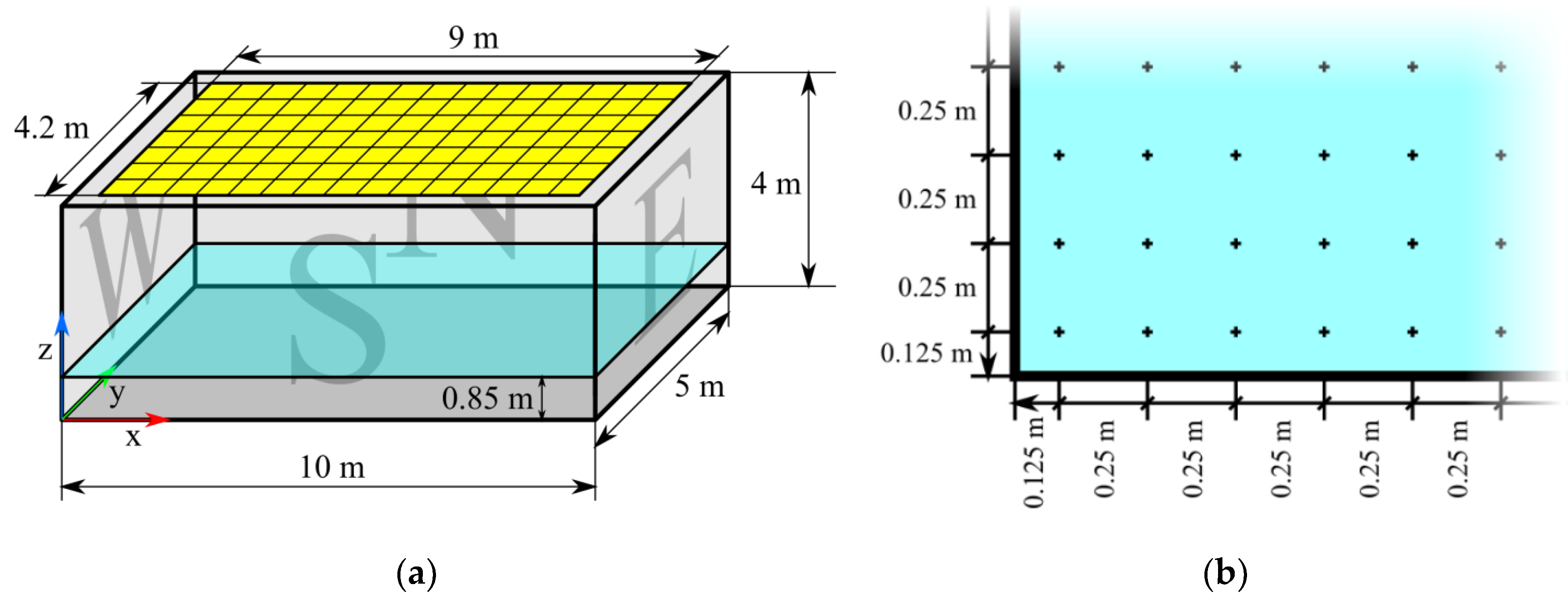
Figure 2.
Increase of average wall illuminances with a single luminaire MSTR SLB 4×18W mounted in the center of the model room’s ceiling depending on the count of light impacts, i.e., number of reflections – 1, calculated using radiosity.
Figure 2.
Increase of average wall illuminances with a single luminaire MSTR SLB 4×18W mounted in the center of the model room’s ceiling depending on the count of light impacts, i.e., number of reflections – 1, calculated using radiosity.
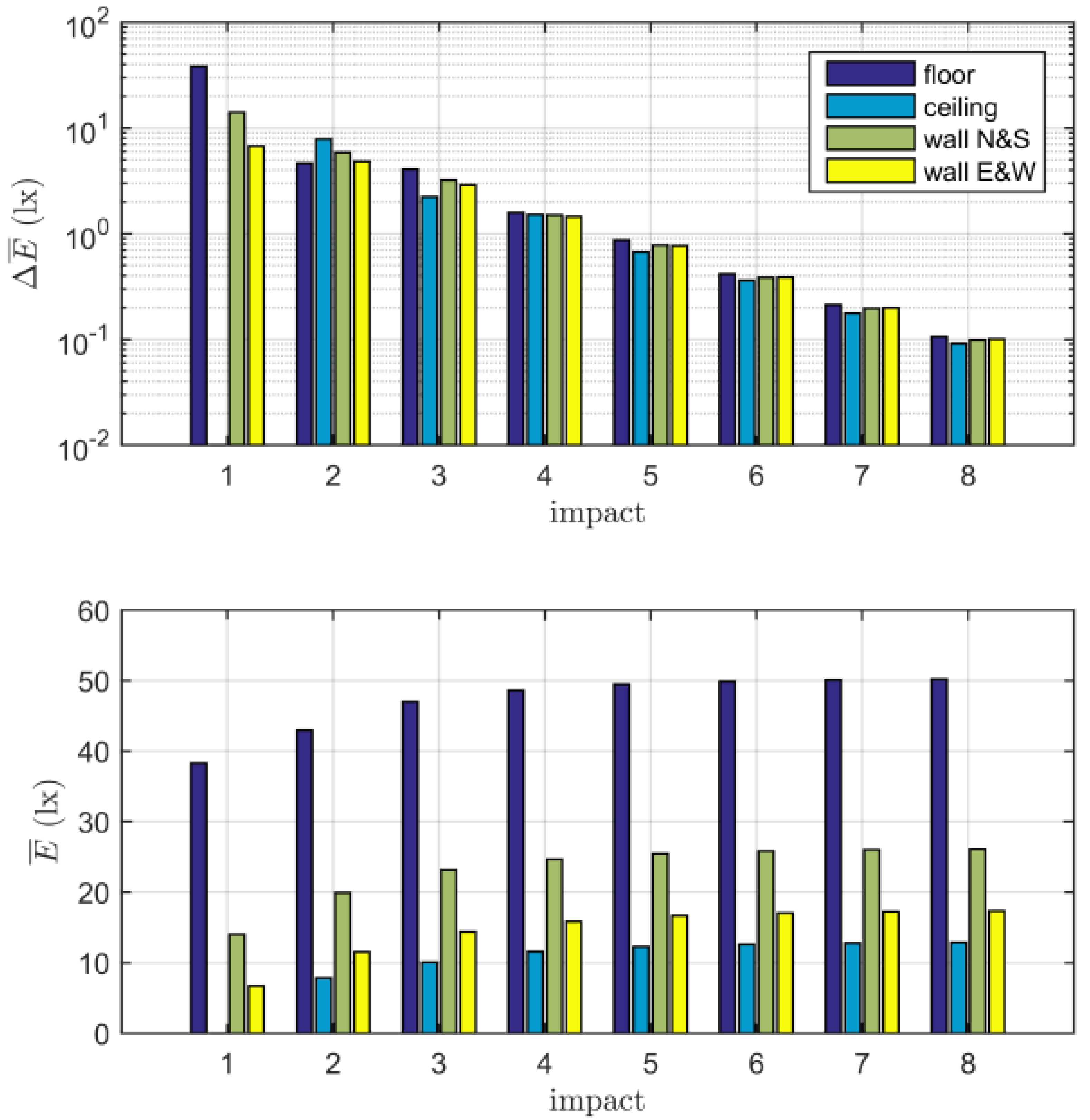
Figure 3.
Used luminaire types from the manufacturer Trevos, their luminous intensity curves, luminous flux ϕ and power consumption P from their respective Eulumdat files: (a) TT LED ϕ = 4340 lm, P = 33 W; (b) PSV PISA SDK T8 OP ϕ = 2970 lm, P = 72 W; (c) PSV PISA SDK T8 PAR ϕ = 3132 lm, P = 72 W.
Figure 3.
Used luminaire types from the manufacturer Trevos, their luminous intensity curves, luminous flux ϕ and power consumption P from their respective Eulumdat files: (a) TT LED ϕ = 4340 lm, P = 33 W; (b) PSV PISA SDK T8 OP ϕ = 2970 lm, P = 72 W; (c) PSV PISA SDK T8 PAR ϕ = 3132 lm, P = 72 W.
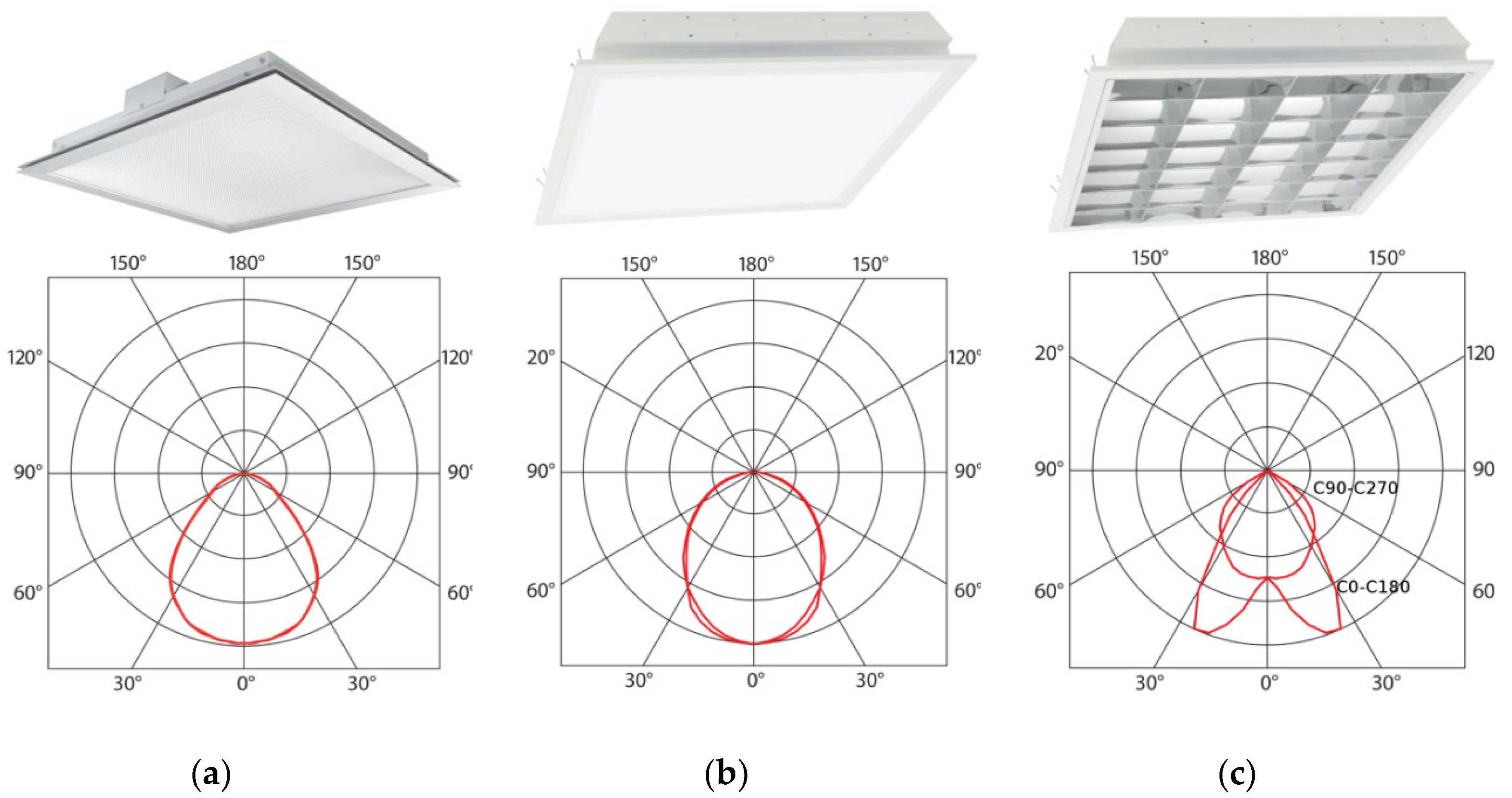
Figure 4.
Custom crossover, switching three luminaires after the selected position (dotted vertical line): take content of parent X’s string and step 1) replace values at positions of three 1s with values from parent Y (green), step 2) replace values at positions of three 1s from parent Y (blue): (a) Offspring with preserved luminaire count; (b) Offspring with reduced luminaire count (one less).
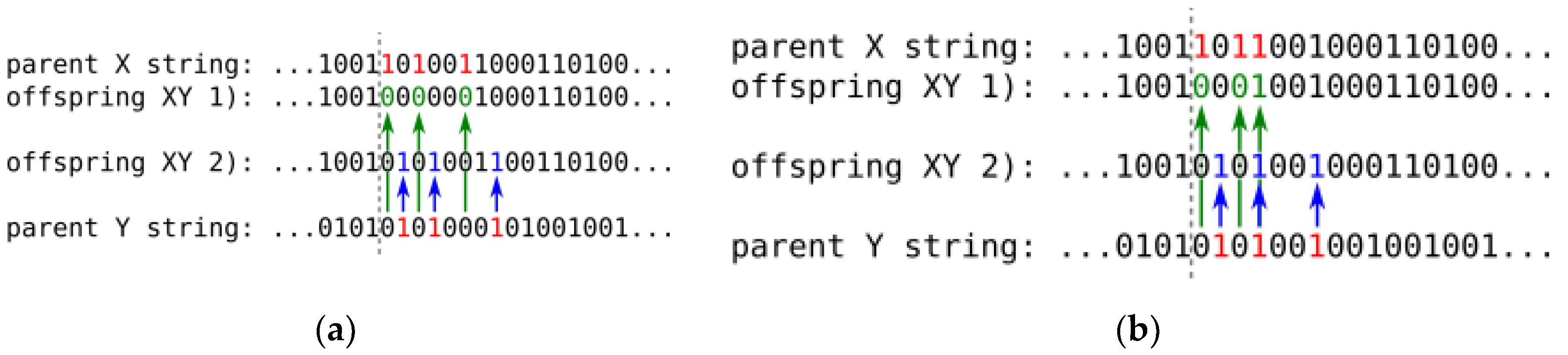
Figure 5.
Top-down view of the model room with black-yellow circles representing luminaire positions in the ceiling plane and isolux diagram of the reference plane (initial illuminance values): (a) TT LED; (b) PSV PISA SDK T8 OP; (c) PSV PISA SDK T8 PAR.
Figure 5.
Top-down view of the model room with black-yellow circles representing luminaire positions in the ceiling plane and isolux diagram of the reference plane (initial illuminance values): (a) TT LED; (b) PSV PISA SDK T8 OP; (c) PSV PISA SDK T8 PAR.
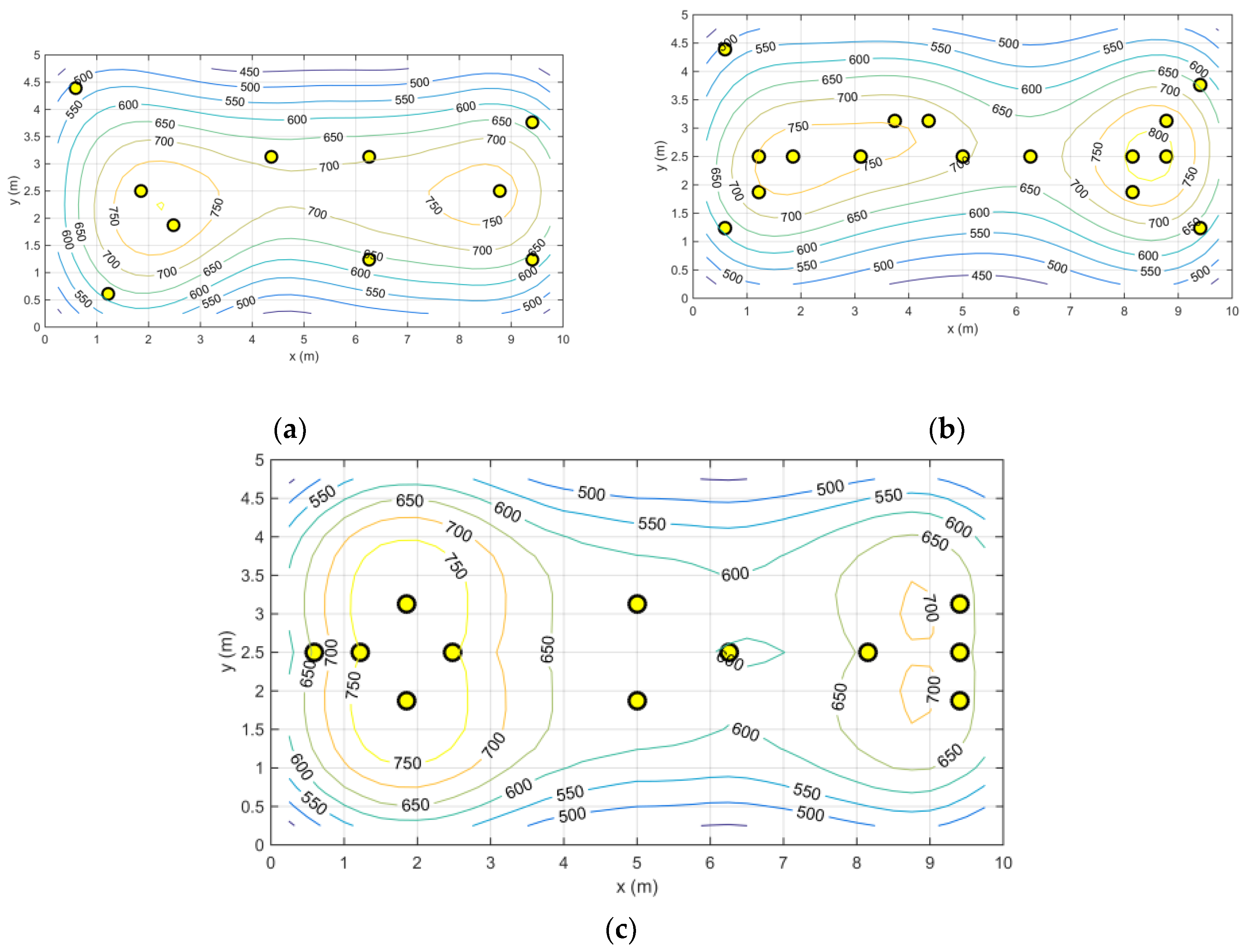

Table 1.
Genetic Algorithm Settings.
| First Population | Random logic vectors |
| Termination Cond. | Defined count of generations |
| Count of Gen. | 500 |
| Population Size | 500 |
| Parent Selection | Tournament 1 of 4 |
| Survival Selection | Elitism |
| Recombination Type | One point, random count of 1 |
| Recombination Prob. | 90% |
| Mutation Method | Bit inversion & Permutation |
| Mutation Prob. | 1% |
| Permutation Prob. | 10% (perm. ≥ 1) 0.349% (perm. ≥ 2) 0.004% (perm. = 3) |
Table 2.
GA output examples, where is the total luminous flux and the total power consumption of all installed luminaires of the given output solution.
Table 2.
GA output examples, where is the total luminous flux and the total power consumption of all installed luminaires of the given output solution.
| Luminaire Type | Count | ||||
|---|---|---|---|---|---|
| TT LED | 10 | 504 | 0.68 | 43400 | 330 |
| PSV PISA SDK T8 OP | 16 | 505 | 0.67 | 47520 | 1152 |
| PSV PISA SDK T8 PAR | 12 | 500 | 0.70 | 37584 | 864 |
Disclaimer/Publisher’s Note: The statements, opinions and data contained in all publications are solely those of the individual author(s) and contributor(s) and not of MDPI and/or the editor(s). MDPI and/or the editor(s) disclaim responsibility for any injury to people or property resulting from any ideas, methods, instructions or products referred to in the content. |
© 2024 by the authors. Licensee MDPI, Basel, Switzerland. This article is an open access article distributed under the terms and conditions of the Creative Commons Attribution (CC BY) license (http://creativecommons.org/licenses/by/4.0/).
Copyright: This open access article is published under a Creative Commons CC BY 4.0 license, which permit the free download, distribution, and reuse, provided that the author and preprint are cited in any reuse.


