Submitted:
30 July 2024
Posted:
30 July 2024
You are already at the latest version
Abstract
A topological representation theory of chiral spin liquid is proposed to unify the integral and fractional quantum Hall fluid based on hyperbolic geometry, knot lattice and Thurston's train track theory. The integral and fractional Hall resistivity obeys an exact unified equation, $R_{xy} = (h/e^2)B_{e}$, $B_{e} = (n+\nu)^{-1}$, with respect to the bulk energy gap ${\Delta}E = {\hbar{e}B_{e}}/{Mc}$. The Wen-Zee matrix formulation of topological fluid for quantum Hall effect is constructed by topological surgery and train track. The chirality of spin liquid is spontaneously distinguished by Jones polynomial. The integral Chern number for Hall conductance is fractionalized by generalizing Thurston's train track to folding laminations in three dimensions, which spontaneously bring fractional quantum Hall fluid and anyons into three dimensions and provided an theoretical explanation on the competing fractional quantum Hall states. The many body system of interacting fermions or bosons are mapped into many interacting liquid droplets that interwind into knot lattice, which provide an effective topological representation for superfluid and superconductor, the strange metal state in superconductor is explained by topological dislocation and topological surgery. The Kauffman decomposition rule in knot theory is extended to describe the topological relations between different two dimensional manifolds, which further reveals the non-trivial relationship between the partition functions of pairing fermions and free electrons. The minimal energy state is the most stable topological state, even thought it maybe shares the same topological number with the excited states. The topological representation theory predicts a circular motion of electrons in hyperbolic space, that is implementable and testable by inhomogeneous magnetic field in three dimensions. The folding lamination representation of topological quantum fluid provides an promising implementation of string theory in high energy physics.
Keywords:
Topological order
; Spin liquid
; Quantum many body system
; knot
; Train track
1. Introduction
Landau’s symmetry-breaking theory is a fundamental law on the nature of phase transitions, offering a comprehensive understanding of the collective phases in many-spin systems. However, this theory does not extend to the spin liquid state, a phenomenon that emerges from quantum frustrated states within the Heisenberg model and has been postulated as a mechanism underlying superconductivity [1]. The chiral spin liquid phase, a characteristic feature of the fractional quantum Hall effect (FQHE) [2], also remains outside the theoretical framework provided by Landau’s symmetry-breaking theory. The Chern-Simons field theory and tensor category theory were proposed as effective theoretical tools for classification of topological order of spin liquid [3]. Despite these advances, the quest for a universal theory for topological order in condensed matter physics continues to be a formidable challenge. Furthermore, the quantization of integral Hall conductance, a problem that has puzzled mathematicians for the past four decades, remains unresolved [4], with the fractional Hall conductance posing an even greater enigma.
An universal topological order theory should provide an exact quantification for both integral and fractional quantum Hall conductance in a self-consistent way, and reveal the topological nature of quasiparticles in spin liquid. The quasiparticles (usually termed as anyon) in fractional quantum Hall fluid carries fractional charge [5] and exotic statistics, is one of the most exotic quasiparticles in condensed matter physics since 1980s [6][7][8][9], showing promising application in topological quantum computation [8] and exploring new topological matters [10].
In this article, the knot lattice model [11] and topological path fusion model [12] are combined to extend the Thurston’s train track theory [13][14] and Witten’s topological quantum field theory [15] into an universal topological representation theory of chiral spin liquid. This topological representation theory provides an unified framework for both integral and fractional quantum Hall conductance, as well as a topological fluid implementation of Jain’s composite fermion theory [16] and Wen-Zee matrix formulation for fractional quantum Hall effect [17]. In this topological representation theory, a quantum particle is modeled as oscillating quantum droplet that continuously deforms into different geometry by keeping its topology invariant. These elongated quantum droplets intertwine to form train tracks in topological fluid. Interacting droplets also collide with one another to fuse into a knot lattice in excited states, which disintegrates into many isolated droplets at high temperature. The mathematical theory of Thurston’s train track [13][14] and knot theory [18][19] provides a rigorous foundation to capture the most important characters of topological fluid on knot lattice.
This articles is organized as follows: in section II, the topological representation of spin liquid on lattice is constructed by knot lattice and train tracks. An unified topological representation theory of integral and fractional quantum Hall fluid is established and extended into three dimensions. In section III, the topological representation theory of anyon in three dimensions is developed through folding laminations. In section IV, the knot lattice theory of chiral spin liquid is developed for quantum many body system in two dimensions to explain the topological phase of fermions pairing and topological superconductor.
2. The topological representation of chiral spin liquid in fractional quantum Hall effect
When the kinetic energy of quantum particles is highly suppressed near zero temperature, many interacting quantum particles collectively acts as topological fluid, since the thermal de Broglie wavelength of a particle can grow up to thousands of times larger than the radius of point particle. We modeled a point particle as a quantum droplet that is stretched into a long ribbon loop, covering the propagation path of point particle following Bohm’s quantum potential [20]. This quantum droplet carries all physical information of a point particle, such as spin, mass, momentum and so on. Many neighboring droplets fuse into one big droplets when temperature decreases. A big droplet also breaks apart into many small droplets under thermal fluctuations. A quantum fluid ribbon winds around another one or twist itself into knot lattice, providing an effective topological representation of quantum fluid.
2.1. The topological representation of spin by knot
The classical Ising spin is modeled as a rotating quantum fluid droplet, featuring two topological defects at the north and south poles, each carrying an identical winding number (Figure 1a). This Ising spin characterize the angular momentum of a rotating charged fluid, which is ideally simplified into an electric current loop (Figure 1b). The Ising spin represents the two opposite states of magnetic dipole moment (Figure 1b). This topological representation of Ising spin satisfies the topological constraint that the sum of the winding numbers equals the Euler number (or Chern number) of the underlying manifold, . The spherical surface of quantum droplet results in . Duan’s topological current theory [21] suggests there exist a topological line defect along which the density of wave function vanishes (Figure 1a),
where the vectorial velocity field that is tangential to the surface of the droplet. The line defect connects the north pole and south pole. Even though the two topological defects carry the same topological charge, but are assigned with opposite magnetic charges (Figure 1c). Free spins without interaction are represented by directed loops without intersections (Figure 1d). Interacted spins are represented by intersecting loops(Figure 1e-h), i.e., cutting each loop current to generate two ending points and glue them with the open endings of another loop (Figure 1e-h). The ferromagnetic coupling is represented by one giant loop made of the fusion of two small loops without self-crossings (Figure 1e). For the antiferromagnetic coupling, the self-crossing of the giant loop made of two nearest neighboring loops is inevitable (Figure 1f). Different crossing states are characterized by chiral index, , where indicated a positive chirality that the four fingers of the right hand first point into the direction of the current above the crossing point and then bend to the direction of the current underneath the crossing point (Figure 1g), while the opposite case is labeled by a negative crossing index (Figure 1h).
A classical rotating droplet is a good representation of Ising spin, but is inadequate to take into account of the phase factor of a quantum particle. A quantum fluid droplet is described by a wavefunction that obeys Schrdinger equation . The Schrdinger equation is equivalently transformed into a pair of fluid dynamic equations by Bohm [20],
The quantum character of a particle is governed by the potential combination of a classical potential V and the well known Bohm potential ,
Here we substitute the identity equations,
into the Bohm potential Eq. (3) to decomposes into the sum of two terms,
The Bohm potential approaches to negative infinity at the zero points of wave function . For a nonzero wave function , the first term on the right hand side of Bohm potential Eq. (5) vanishes. The second term of Bohm potential Eq. (5) is determined by the gradient of wavefunction. The Bohm potential turns into zero at the extremal points of wavefunction, i.e., . According to Duan’s topological current theory [21], the sum of topological charges of zero points of wavefunction is determined by the topology of spacetime manifold. Therefore a quantum particle is born to carry the topological information of the space time manifold at , which usually is eliminated in local dynamics. The Bohm potential reaches the minimal (maximal) point when the gradient of wavefunction is positive (negative). The particle moves along the minimal points of Bohm potential under the mathematical constraints . The quantum fluid droplet deforms into different oscillating modes following Bohm potential. The velocity field on the surface of quantum droplet is defined as
The velocity field as showed in Figure 1a shows two topological defect on the north pole and south pole of the spherical droplet. The spherical droplet deforms into a solid torus when the line defect penetrate through the north pole, south pole and the mass center. A moving particle going around the topological line defect twice provides an effective representation of spinor wavefunction for (Figure 2a),
An equivalent topological deformation of solid torus is Mbius strip. The edge of the Mbius strip locates along the extremal points of Bohm potential. An electron winds around the topological line defect to form a closed path in Figure 2a. The periodicity of the other phase factor is still . The eigenvalues of the spin operator are , which represents the chirality of flowing current in Mbius strip.
Unfolding the edge of Mbius strip into an ∞-shaped knot preserves the topology of quantum fluid torus and the periodicity of spinor wavefunction. The Figure 2a represents the wavefunction of topological spin state , which defines a topological representation of electron spin . The spin states of ∞-shaped knot crossing, and , are represented by complex wavefunctions with four components,
It must be pointed out that magnitude of wave function for knot crossing is not normalized to unity, instead it is normalized by Jones polynomial, . Figure 2b (Figure 2c) represents the two components of wavefunction for topological spin state with (). The tangential velocity of circling fluid in the knots of Figure 2b-c is determined by the gradient of phase field of wavefunction. Opposite gradient fields generate opposite tangential flow fields. A crossing state in Figure 2a-b transforms into uncrossing state in two different ways, as showed in Figure 2d-e. The uncrossing states are topological vacuum states, denoted by and ,
Both the topological crossing basis and vacuum basis are not normalized and orthogonal, but a set of orthogonal basis always exists to expand the two sets of topological basis into the same Hilbert space,
The conventional Jones polynomial are projected into the orthogonal basis . The eigenvalue of topological spin with respect to vacuum states is zero, or . Once the two currents are oriented to form the horizontal vacuum state , the vertical vacuum state is forbidden under continuity constraint of topological invariant. The magnitude polynomial of the topological spin states transform into one another following Kauffman decomposition rule in knot theory[18],
which are further reformulated into matrix equation,
Substituting the orthogonal Eq. (9) of topological vacuum states into the decomposition Eq. (12) yields the transformation equation between the crossing basis and uncrossing basis ,
The basis transformation equation an unitary matrix, which is expanded by the generators of SU(2) group,
where the crossing state vector and uncrossing state vector are denoted as
Both the crossing state and uncrossing state have four open endings. In order to form closed path that is topologically equivalent to circles, edge states with two open endings are introduced as following.
where , represents the left, the right, the top and the bottom edges respectively. The topological edge state of single current branch locates along the edge of knot lattice. Once the edge current configuration is fixed, its collective configuration remains invariant when the bulk knot lattice transform from the crossing basis to the uncrossing basis. The product of two edge states of opposite semicircles, or , are defined as closed vacuum state . The closed vacuum state can be represented by unit matrix. The simplest representation of is U(1) group element,
In knot theory [18], the polynomial with respect to the combination of a closed loop and general link is defined as
This decomposition rule is derived from two coupled crossings, that decomposes according to Eq. (11).
Two coupled crossings with independent topological spin numbers generate four possible crossing states, , , and as shown in Figure 3. Unlike the four independent basis of two coupled spins in quantum mechanics, the two crossings with opposite topological spin are transformed into the same product state of two vacuum states under Reidemeister moves,
where is the operator of the Reidemeister move. As showed in Figure 3b-c and Figure 3e-f. Applying the Kauffman decomposition rules for the four crossing basis transforms them into four vacuum basis of two coupled spins,
In mind of the orthogonal relations between different basis, i.e., , , , the transformation matrix of knot polynomial is mapped into the transformation matrix between the two four dimensional basis vectors,
The polynomial vector of N coupled crossings transforms into N coupled uncrossings following the same decomposition rules as above, . The transformation matrix U is a matrix of Kauffman polynomial, which is equivalent to Jones polynomial.
Beside the quantum wavefunction representation of knot, the knot lattice has a straight forward representation by matrix of quantum creation and annihilation operators. Cutting one cross out of its surrounding network generates four open endings in Figure 4a. The directed flow along the current line is represented by the product of a creation operator and an annihilation operator, i.e., and . The crossing in Figure 4a is represented by a matrix equation,
where h is the hopping rate. is fermion operator and obeys anticommutative relations,
The hopping rate in Eq. (22) is multiplied by a topological phase term , where the topological spin is quantified by
where is the gauge field potential along the current lines. The two crossing current lines that avoid touching each other always bend into opposite directions, since the four ending points are projected into the same plane. When the topological spin flips to by exchange the top and bottom lines, the divergence field or flips its orientation respectively. The topological spin Eq. (24) is essentially the abelian Chern-Simons action,
defined on a local crossing. The quadratic fermion operator Eq. (22) is equivalent to Hamiltonian equation with t measures the kinetic energy of a hopping particle. Therefore the representation matrix is termed as topological Hamiltonian matrix here. The topological vacuum state for two uncrossing current lines in Figure 4b is also represented by four fermion operators which interact with one another following the Hamiltonian equation ,
Since the two current lines in vacuum state avoid crossing each other, the topological spin is defined by the product of the divergence field of the two arc lines,
The divergence of the two arcs in Figure 4b are oriented in the same direction, denoted by the black dot surrounded by a circle, therefore the eigenvalue of topological spin is . The topological spin Eq. (27) for vacuum states shares similar definition with the second Chern number in four dimensional manifold,
The conjugate of is represented by the same two arcs in Figure 4c, in which both the flow field and divergence field of the two arcs are reversed simultaneously to preserve the value of topological spin . When the two arcs in vacuum state generate opposite divergence fields, the topological spin of vacuum state is . For example, the Figure 4d is composed of two arcs with opposite divergence, the topological spin in the Hamiltonian matrix,
is , which is invariant in the conjugate vacuum state , because both the two opposite divergence fields reversed their orientations (Figure 4e).
The open endings are connected by edge currents to form a closed loop. In the quantum operator representation of knot, the edge current are also the product of a creation and an annihilation operator. The Hamiltonian matrix of the "8"-shaped knot in Figure 4f reads
where is the hopping rate of edge current. A ∞-shaped knot is generated by adding the other two edge states, and , on the cross in Figure 4a. The corresponding Hamiltonian matrix is
The ∞-shaped knot and "8"-shaped knot share the same topology but are distinguishable by the Hamiltonian matrix. This Hamiltonian matrix representation of knot lattice has a straight forward extension to more complex knot lattice. For example, the chiral flow in the knot lattice of Figure 4h is described by the chiral Hamiltonian matrix
where is the complex hopping rate. This topological Hamiltonian representation spontaneously eliminated the intersecting current lines out of knot lattice (Figure 4i), where the product terms of four fermion operators emerges. The dimension of the Hamiltonian matrix of a knot lattice is determined by the total number of nontrivial endings. Each ending represents one fermion particle. This quantum representation provides a natural explanation on the assumption in knot theory, i.e,. The collective quantum state of a trivial circle composed of N endings is denoted as
where is the occupation number on the ith ending. The Hamiltonian matrix representation of the circle is dimensional diagonal matrix. The knot polynomial is derived from determinant of the Hamiltonian matrix,
If the occupation number at any one ending points is zero, the track chain remains open, the polynomial equation of circle is spontaneously zero.
The topological Hamiltonian for a knot lattice is independent of dynamics of interacting crossings. Interacting crossings in knot lattice is described by dynamic Hamiltonian. When the crossing states transform into another crossing states under thermal fluctuation or external field stimuli, the knot lattice is in superposition state of different crossing patterns. For the simplest superposition state of single crossing with opposite topological spin , the wavefunction is denoted as , the density matrix is defined as
counts the probability of the cross in the state with topological spin . counts the probability of the cross state with . or counts transition rate between the two opposite crossing states. The density matrix obeys the Heisenberg equation of motion,
A general Hamiltonian for the crossing transition dynamics is
measures the reversing frequency of the chiral current in knot. measures the hopping strength between opposite crossing states. Notice here the Hamiltonian and density operator are expressed by the same basis. If the density operator is expressed by superposition state of topological vacuum basis
The density matrix in the vacuum space is an unitary transformation of the density matrix in the crossing space,
The vacuum state is transformed into topological crossing state according to the inverse of Eq. (14), . The dynamic Hamiltonian Eq. (37) in the crossing basis also has an equivalent expression in the vacuum basis,
The dynamic Hamiltonian Eq. (40) is self-consistently applicable on a density matrix originally expressed by topological vacuum states. If the quantum system is a hybrid four level system of two crossing states and two vacuum states, the corresponding dynamic Hamiltonian is expressed by both the crossing basis and the vacuum basis,
The topological invariant polynomial maps the vacuum basis to the crossing basis, providing a topological constraint equation on the hopping process between vacuum state and crossing state. The dynamic hopping in non-topological electron fluid is governed by quantum electrodynamics. The hopping process between different energy levels of topological fluid must take the knot invariant into account.
The Kauffman polynomial of knot lattice is equivalently mapped into Jones polynomial by multiplying with the writhing number, i.e., . The Jones polynomial is equivalent to an evolution operator that maps the initial crossing states of linked knot lattice into all possible full loop states with inequivalent topology,
where denotes the ith full loop state. For the initial knot crossing state of the right handed trefoil knot in Figure 5, , decomposing the three crossings of leads to eight possible full loop states,
The four vacuum states with two loops, , , and , are topologically equivalent. The three vacuum states with one loop, and , share the same topology. There is only one vacuum state with three loops, . The power indices in Jones polynomial with respect to the right handed trefoil knot in Figure 5 encoded the total number of topologically inequivalent loops state,
where . The Jones polynomial of the left handed trefoil knot reads . The Jones polynomial is independent of the sequential order of decompositions of the three crossings. Permutating the spatial locations of the three crossings in decomposition always leads to the same eight vacuum states and the same Jones polynomial. The Jones polynomial of the left handed trefoil knot is expressed by the same counting sequence , except that the variable t is replaced by in Eq. (44). In the Ising model of knot lattice, the polynomial variable t is a Boltzmann factor with respect to different energy, . The value of local spin with respect to crossing state is () in the right (left) handed trefoil knot. This physical interpretation coincides exactly with the rigorous proof in knot theory. On the other hand, different vacuum states also evolve into different excited states under thermal fluctuation, i.e., different loop configurations evolves into different knot lattices, therefore the Jones polynomial builds a robust bridge between zero energy states and excited states with non-zero spins, as long as thermal fluctuation does not destroy the topology of knot lattice.
The right handed trefoil knot in Figure 5, , is one of the eight crossing basis, with . The vacuum basis also has eight components, with . The matrix of Jones polynomials is a transformation matrix from the vacuum space to the crossing space,
This transformation equation holds for the most general case of a knot lattice with N crossings. The Jones polynomial matrix encodes all possible series decay from a knot lattice of crossings to a lattice of full loops, because the knot lattice with crossings is in excited state and unstable, the fluctuating current lines inevitably touch each other at some time point and fuse into vacuum states. The full loop state is the most stable state against thermal fluctuations.
The Jones polynomial determines the partition distribution of loop states with different number of loops in zero energy state. In the highly degenerated Hilbert space of zero energy state with respect to the right handed trefoil knot (Figure 5), the loop states with three loops contributes the major part to the Jones polynomial. On the contrary, the three loop states contributes the minimal part to the Jones polynomial. This conclusion holds for link on a general knot lattice with many crossings. Only chiral flow in knot lattice survives during thermodynamic evolutions, the flow in knot lattice with opposite chirality exponentially decays to zero (as shown in Figure 6). Therefore the series decay of knot lattice prefer choosing a chiral path.
The energy of the three crossings of trefoil knot Figure 7a is quantified by an effective Hamiltonian, . The high energy state is defined by three crossing states with the same positive topological spins across the cutting surface in Figure 7b. The low energy state is a crossing state formed by two fluxes without penetrating through the boarder. Every topological vortex costs at least two continuous braiding operations as well as two identical crossing states. The total energy of many topological vortices on boarder surface is counted by the linking number of the knot lattice of magnetic fluxes,
The eigenenergy of Hamiltonian Eq. (46) counts the total energy of the 12 topological vortices in Figure 7b. When the docking points of the four fluxes in cross section or are connected to fuse the four separated flux loops into one flux loop, the knot pattern in Figure 55e realizes a chiral trefoil knot in Figure 7a. The flux segment that connects the edge points of flux No. 2 and flux No. 3 cross the boarder surface once, while the edge flux segment has to cross three boarder surface to connect flux No. 1 and No. 4. There are four topological vortices created in the left-hand cross section . On the right-hand cross section , the edge flux connecting flux No. 1 and No. 3 intersect with four boarder surfaces and created four topological vortices swirling around the intersecting point. Four topological vortices are also created along the edge flux segment connecting flux No. 2 and No. 4. There are eight topological vortices in total in the right-hand cross section (Figure 7b). The total number of topological vortices in grows with respect to an increasing number of periods of braiding.
The Hilbert space of three spin 1 particles is expanded by basic knot patterns, 15 exemplar knots are listed in Figure 8. Every knot pattern is labeled by a general quantum state The left-handed trefoil knot is denoted as The ferromagnetic state represents the right-hand trefoil. The Kauffman bracket polynomial of the left-hand trefoil reads
The Kauffman bracket polynomial of the right-hand trefoil is , in which the parameter A is
The chirality of the trefoil knot is distinguished by the Kauffman bracket polynomial. Since the trefoil knot in Figure 7c is created by braiding operations, the highest power of A in bracket polynomial Eq. (47) is . The fractional quantum Hall state in the cross section of Figure 7c carries fractional charge . Therefore the chiral edge modes in FQHE is distinguishable by Kauffman bracket polynomial. When the ferromagnetic state flips to , the total spin flips to , driving the Kauffman polynomial of the left-hand trefoil into that of the right-hand trefoil. The chirality of trefoil knot is spontaneously mapped into chiral Jones polynomial as well as Kauffman polynomial,
The Jones polynomial is equivalent to Kauffman polynomial under the exact map of variables . The trefoil knot in Figure 7a is mapped to crossing state of three mutually perpendicular fluxes in three dimensions with a special boundary condition (Figure 7c). Both Jones polynomial and Kauffman polynomial can be interpreted as the Boltzman weight of collective spin state with respect to eigenenergy .
At high temperature, a magnetic flux within low magnetic field could cut another flux and reconnect to each other, this dynamic process drives an overcrossing flipping to undercrossing (or vice versa). In the plasma analogy theory of FQHE, the inverse of total number of braiding operations is proportional to effective temperature. At finite temperature, the partition function of three topological spin1 is the sum of Boltzmann weights of all possible collective states of the three crossings,
where indicates all possible collective spin configurations of three crossings. The simplest formulation of the total energy of three crossings is . The coupling interaction between crossings leads to more complex energy formulations. The partition function with is not a topological invariant due to the absence of boundary condition with respect to each knot state. The Kauffman bracket polynomial is the eigenfunction with respect to eigenenergy . The Hamiltonian of three crossings is equivalent to a renormalized writhing number of single loop, . Therefore topologically nonequivalent knots are classified by writhing number, i.e., the total spin, The partition function of three crossings is the sum of the Boltzmann weights with respect to different knots states,
where is the writhing number of the nth knot states. The Boltzmann weight measures the occupation probability of a knot state at finite temperature.
The knot polynomial of all possible knots that are generated out of three crossings is derived by Kauffman decomposition rules in knot theory,
where and . The polynomial of knot including closed loops are decomposed following the conventions, and . In Figure 8, the knot state of represents two linked loops, () represents two loops circling in the same (opposite) direction. The writhing number equation for is equivalent to the linking number of two interlocking loops, . The Kauffman bracket polynomial of nontrivial knot states in Figure 8 are derived from Kauffman decomposition rules,
An implementation of the knot variable A by periodical wave transforms the bracket polynomials into the superposition wavefunction. The simple bracket polynomials are eigenfunctions of angular momentum operator . The eigenvalue of equals to the number of braiding operations as well as the writhing number of single loop, i.e., or . The knot states with the same topology in Figure 8 are represented by the same Kauffman polynomials,
However the knot states with the same topology do not share the same energy due to the geometric bending or twisting of the loop. Three coupled spins generate 64 possible collective states in total. The total number of knot states with respect to the writhing number is denoted as and counted as following,
The energy of knot is assumed to be proportional to the writhing number , . The thermodynamic partition function of three coupled topological spins is
The free energy and thermodynamics entropy are spontaneous output of this partition function,
The entropy approaches to zero when temperature decreases to zero (Figure 9). The three knot crossings tend to orient their spins in the opposite direction of external field h. There is no coupling between different crossings. Therefore the entropy of three free crossings (as showed in Figure 9) is similar to that of three free Ising spins. The crossings in knot lattice are always strongly correlated with one another. It is a reasonable assumption that the left handed trefoil knot shares the same energy as the right handed trefoil knot in absence of external field. Therefore the total Hamiltonian of knot lattice in external field is the sum of the coupling interaction and the interaction with external fields,
where is the total number of crossings. The output energy of acting on the knot configurations in Figure 8 are listed as following,
The eigenenergy of states with writhing number includes the coupling interaction between a positive crossing and a negative crossing, which is spontaneously eliminated by Hamiltonian . The corresponding thermodynamic partition function of a knot with three crossings reads
The coupling interaction between crossings introduced non-topological factors into partition function. The thermodynamic entropy with respect to is similar to entropy Eq. (56) on the cross sectional surface of , but expands into the extra dimension defined by coupling strength J.
The knot configurations with different eigenenergy (i.e. writhing number) may share the same topology. The knot with only one crossing keeps its topology invariant when it hops from excited state to ground state under thermal fluctuations. The topology experiences a sudden change when the knot hops from the left-hand or the right-hand trefoil knot to ground state with . The dynamics hopping between the two chiral trefoil knot states, and , is governed by the effective Hamiltonian,
Notice here , the Jones polynomial wavefunction is expressed by orthogonal basis,
The density operator of a mixed state with the probability being and probability being is defined as
where and . The uncertainty of the mixed state is measured by the von Neumman entropy,
Because the right hand trefoil knot state is not a pure state in the orthogonal basis space, itself is a mixed state in the orthogonal basis space. Substituting the Kauffman polynomial Eq. (54) into the von Neumman entropy of the pure state yields
Substituting the Boltzmann factor into Eq. (65) yields the von Neumman entropy that evolves with temperature,
Figure 10 shows that the von Neumman entropy of the right hand trefoil knot reaches the maximal value before it decays to zero near zero temperature. The entropy of the left hand trefoil knot vanishes at finite temperature (Figure 10). The entropy of other pure states is derived in a similar way of combining Kauffman polynomial Eq. (54) and the von Neumman entropy Eq. (64). The entropy of the single loop state (as shown in Figure 8) is constantly zero, so does its topological equivalent configuration in Figure 8.
A complex topological fluid is composed of many different knots. These knots entangle with one another to form a knot lattice when temperature drops. As temperature gradually increases, the viscous topological fluid gains more kinetic energy to breaks into discrete flowing zones, decomposing a knot lattice into many isolated small loops. The Jones polynomial governs the topological decomposition process, offering an effective density operator to measure the number of all possible states with respect to certain number of loops. For a general knot lattice with n crossings, the knot polynomial wavefunction is not the direct product of the polynomial of single crossing, instead it is a nonlinear function,
where denotes topological index of local crossing state. The two crossing states and topological vacuum state at the ith lattice sites are denoted as a vector of two components,
The crossing wavefunction transform into the uncrossing wavefunction under the decomposition operator , which is derived from the Kauffman decomposition rule in knot theory,
The modular square of the crossing wavefunction is defined as the conventional Jones polynomial or Kauffman polynomial, . As a result, the transformation operator between Jones polynomials is the product of the decomposition operator and its conjugate operator ,
acts on the polynomial with crossings . The polynomial with crossings is further decomposed into the sum of polynomial with crossings,
The iterative decomposition operation generates a series of Jones polynomials that maps the knot lattice with i crossings into free loops configuration. The Jones polynomial of knot lattice with n crossings reads,
The von Neumman entropy of the knot lattice with n crossings is
The Jones polynomial is a topological invariant, as a result, the entropy Eq. (73) is the topological entropy of knot lattice.
2.2. The knot invariant of chiral spin liquid of one dimensional spin chain
Every electric knot interlocks with an induced magnetic knot current. The electric knot with only one self-crossing interlocks with a simple magnetic loop (Figure 11a) without self-crossing following electromagnetic induction effect. The link of this electric loop and magnetic loop is characterized by a topological invariant number—Linking number,
where is the total number of positive (negative) crossings. The link in Figure 11a has a linking number . Flipping one of the two spins in Figure 11a either unties the self-crossing into parallel lines (Figure 11b) or generates one more crossing both on the electric loop and magnetic loop (Figure 11c). This linking number is invariant during the flipping process. For a more general case of many coupled spins along one dimensional chain, the antiferromagnetically coupled spins is either represented by a knot lattice of electric loops or a topologically equivalent magnetic knot lattice (Figure 11 d), there exist an exact one-to-one correspondence between the electric knot lattice and magnetic knot lattice. This exact correspondence also holds for a ferromagnetically coupled spin chain as well as an arbitrary spin liquid state.
The combination of a knot lattice of magnetic fluxes and Thurston’s train track pattern constructs an unique topological representation of a spin liquid state. Figure 12a shows an exemplar spin liquid state, where Ising spins are represented by arrows pointing up or down. Based on the convention of constructing magnetic knot lattice in Figure 11 a-b, two antiferromagnetically coupled spins are represented by two parallel magnetic lines, while ferromagnetically coupled spins are represented by crossing magnetic lines. A magnetic line segment always connects two poles of the spin arrows with opposite magnetic charges (Figure 12c). The linking number of the knot lattice formed by connected magnetic lines is independent of local direction of the line segments, therefore the knot lattice is further mapped into the same knot lattice generated by two magnetic fluxes that are oriented in opposite direction, as represented by the blue and red lines in Figure 12d. When the two magnetic fluxes are immersed in an electronic fluid, the flowing electron fluid form laminar layers winding around the two magnetic fluxes under the propulsion of Lorentz force, . To reconstruct exactly the same knot lattice as Figure 12d, the left endings of the two magnetic fluxes are first fixed, and their corresponding right endings are braid in a designed protocol so that the cross section of the right ending of the electric laminar layer generates a winding path that is described by a topology theory called Thurston’s train track (Figure 12e). As an application of Thurston’s train track theory, the number of layers of electric line segments on the two opposite sides of the magnetic fluxes are counted and labeled by and correspondingly. An integral electric charge splits into fractional charges passing thorough the train tracks,
leading to fractional Hall resistivity in fractional quantum Hall effect [12]. The train track pattern in Figure 12e generates two fractional charges, and .
The train track of electric current on the boundary is a stable topological pattern against local perturbations on spins in the bulk chain. In the exemplar spin configuration of spin liquid state in Figure 13a,
two ferromagnetic domains are separated by a topological kink soliton, (indicated by the orange dash line on the left hand side of the spin pair of red arrows. Flipping the local spin pairs labeled by red arrows does not annihilate the kink,
but transferred it to the right hand side. Therefore, and share the same eigenenergy, . Flipping the local spin pair labeled by red arrows in Figure 13b annihilates two kinks simultaneously and leaves only one kink behind.
The eigenenergy of this spin liquid state is the energy gap of one kink, . Topological kink solitons always generate or annihilate by pairs to keep the total topological charge invariant. The linking number of the knot lattice is invariant during these local flipping operations in the bulk, so does the train tracks on the boundary. The fractional charges on the boundary is quantized by the topological linking number,
where is the total number of effective braiding operations. As proved by the topological path fusion theory of fractional quantum Hall effect [12], this fractional charge straightforwardly determines the fractional Hall resistivity,
Therefore, the fractional Hall resistivity is quantized by topological linking number, this quantization rule is different from that of integral quantum Hall effect that is quantized by Chern number [22].
The linking number of the knot lattice determines the energy gap of the spin liquid state, which is similar to the Haldane gap in one-dimensional Heisenberg chain with spin S antiferromagnetic coupling, i.e., an unique gapped ground state exists for an integral Spin [23]. Here an integral linking number indicates two fully separated magnetic fluxes without any touching point (Figure 14a). For half-integral linking number, there always exist two vortices penetrating through the electric laminar layer that acts as a boundary layer separating the two magnetic fluxes (Figure 14b). The two vortices glue the two magnetic rings into one big ring with a self-crossing point, which is exactly the boundary of mbius strip. The magnetic current along the boundary of mbius strip represents a topological spin state, and , where represents the two topological vortices that cannot be eliminated by local operations. The local fluctuation of magnetic fluxes can also generate a pair of vortices crossing the electric laminar layer (Figure 14c) with topological spin 0, however this vortex pair is unstable and tend to annihilate each other under thermal fluctuations (Figure 14d). There is no topological vortices on the electric boundary layer for a magnetic knot lattice with an integral linking number, for the exemplar Figure 14e, the knot lattice of two linking magnetic rings generates electric wrinkles with a topological spin . Braiding the magnetic flux segments of spin 0 states three times generates two half integer spin states with opposite spin S = and S = . The fractional charges and on the boundary cross section between the two states S = and S = (Figure 14f) are unstable against local thermal fluctuations, reducing to spin 0 state without topological crossing. The unstable fractional charges can also be generated out of spin state by local braiding (Figure 14f), the sum of a S = 1 state and S = state, however the topological vortex pair is always robust against any local braiding or thermal fluctuations.
The real spin vectors sandwiched in between two magnetic flux lines represent the spins of real particles. The collective order of real spins fluctuate in thermal environment and transform from one collective phase to another. The two magnetic flux lines form a one dimensional knot chain of crossings, the collective order of many crossings in knot lattice is invariant during thermal fluctuation. A local crossing state in knot lattice is equivalent to topological spin 1, . and represents the overcrossing state, undercrossing state and cross avoiding state respectively in Figure 15a. The key difference of topological spin 1 from the spin 1 of real particle in nature is that the zero spin state has two topologically different states, the vertical vacuum and horizontal vacuum states in Figure 15a III-IV, denoted as and respectively. In knot theory, the crossing states in Figure 15a are represented by Kauffman brackets,
In the knot lattice theory of anyons [11], the partition function of a spin 1 state is mapped into a Boltzmann weight factor within external magnetic field h,
which counts the occupation probability of a topological spin 1 on state with eigenenergy . The Boltzmann factors are exactly the corresponding Jones polynomials with respect to different crossing states, satisfying the Skein relationship
where the coefficients in Eq. (83) are
The Jones polynomial is mapped exactly to Kauffman polynomial by redefining the variable A in Kauffman bracket as
The Kauffman brackets Eq. (Figure 8) transforms into brief formulations of Boltzmann distribution,
The Kauffman polynomial of spin zero state measures the probability of finding spin up or spin down,
In statistical physics, the conventional partition function is the sum of Boltzmann weights of all possible states
The magnetization of the knot lattice is topological linking number [11], which is an integer at zero temperature but deviates from integer at finite temperature,
The linking number equivalently counts the total number of braiding, , where counts the total number of clockwise (counterclockwise) braiding. In the train track representation of abelian FQHE, the one dimensional knot lattice of magnetic fluxes is generated by periods of identical braiding, leading to average fractional quantum Hall resistivity ,
Substituting linking number Eq. (89) into Eq. (90) yields average fractional Hall resistivity at finite temperature,
where t is the same parameter in Jones polynomial. At hight temperature, thermal fluctuation drives a local crossing to fluctuate among many different crossing states, different fractional Hall resistivity may appear simultaneously, Eq. (91) measures the average fractional filling factors at certain temperature.
The single crossing of Figure 15 a-II braids the electron fluid surface into a folded lamination with an edge cross section state of . More braiding operations in the same direction twists the single crossing into an alternating knot chain in Figure 15 b, which is represented by Kauffman bracket polynomial,
where represents the overcrossings with . If the left-hand endings of the two fluxes in Figure 15 b are fixed, the right-hand cross section of the alternating knot generates the train track pattern with fractional filling factor,
The Kauffman bracket polynomial is mapped to the eigenfunction of angular momentum operator ,
The eigenvalue of angular momentum records the total number of continuous braiding in the same direction,
Negative indicates braiding operations in opposite direction. The fractional Hall conductivity only exist for the alternating knot chain of Figure 15 b that is confined rigorously in two dimensions, the knot chain is prevented from flipping back to a trivial circle due to dimension reduction. The renormalized Kauffman polynomial of the alternative knot is
where is the writhing number of a twisted circle. Here equals to the sum of the signs of all crossings in the knot chain formed by a circle. The constant value of Kauffman polynomial suggests that the twisted circle shares the same topology with the initial unit circle. The fractional Hall conductivity encoded by alternating knot in Figure 15 b is unstable at finite temperature due to the simple topology.
The collective configurations of many real spins in one dimensional chain can map into the same knot lattice of intertwined magnetic fluxes (Figure 12). In Figure 15 c, the leftmost and the rightmost edge zone of the double hyperbolic surface are covered by ferromagnetic phase of classical Ising spins, while antiferromagnetic phase covers the bulk zone in the middle. If the bulk lattice is composed of an even (odd) number of unit cells, the ferromagnetic phase of the leftmost edge zone orients in the same (opposite) direction to that of the rightmost edge zone (Figure 15 c-d). The collective phases of far separated edge zones in opposite boundaries are strongly correlated, due to the robust topology of two intertwined magnetic fluxes. This topological correlation is stable against local thermal fluctuations unless the magnetic flux line is cut into discrete segments. The two intertwined magnetic flux loops in Figure 15 c transform into two far separated loops under Reidemeister moves, which are represented by Kauffman bracket polynomial . While two interlocking loops in Figure 15 d is equivalent to two magnetic loops linked in a nontrivial way, described by Kauffman bracket polynomial . If the left-hand and the right-hand edges of Figure 15 c-d are fixed, a pair of hyperbolic surfaces of electron fluid lamination with opposite normal directions is generated in the middle zone. Each cross section of the hyperbolic lamination represents a qusiparticle with fractional charge . These quasiparticles are always generated or annihilated by pairs under local fluctuations of real spins in one dimensional chain.
If the collective configuration of real spins in the bulk zone of Figure 15 e are frozen, finite hyperbolic surfaces of electron fluid lamination are generated on the left-hand and the right-hand edge. Topological quasiparticles carrying opposite topological spin and fractional electric charge as are pushed to the edge zone. The linking number of the two interlocking loops in Figure 15 e counts the total number of robust crossings which can not be generated or annihilated by local spin fluctuations, unless the loops are cut to reconnect. The two hyperbolic edges are flattened by opposite braiding operations to the initial braiding orientation in Figure 15 e, the four crossings in bulk zone are transferred to the intertwined magnetic loops in infinity by keeping the topological linking number conserved.
The topological linking number of magnetic flux knot lattice is inadequate to distinguish different boundary states. In Figure 16, braiding the leftmost edge three times in counterclockwise direction around the left normal direction and braising the rightmost edge three times in clockwise direction around the right normal direction maps into monotonic hyperbolic surface generated by five counterclockwise braiding around the left normal direction. The monotonic hyperbolic surface and double hyperbolic surface in Figure 16 share the same topological linking number, but their geometric characters and dynamics of electron on the surface are completely different. Therefore quantum states characterized by topological number are usually highly degenerated.
Inhomogeneous magnetic field folds the electron fluid lamination into non-Euclidean geometry, bending the flat lamination into hyperbolic surface with negative curvature. In Figure 17a, the endings of the flux pairs on the right hand side are fixed. Braiding the endings on the left hand side in counterclockwise direction folds the flat lamination into a hyperbolic surface, which is implementable in experiment by designing a decreasing magnetic field strength from the right hand side to the left hand side. The train track on the left boundary cross section represents fractional filling state . In Figure 17b, both the two endings of the flux pair on the left and right hand side are fixed, braiding the middle points of the two fluxes expands the middle zone of the initial flat surface, generating a double hyperbolic surface on which the filling factors decrease from on the edges to in the middle. Figure 17c shows a more complicate magnetic field configuration, a constant magnetic field strength is homogeneously distributed in bulk, but decreases in edge zones on both the left and right hand side. The initial flat lamination in edge zones are folded into hyperbolic surface by braiding operations on the left and right endings of the flux pair in counterclockwise direction. The filling factor decreases from the bulk to the edge, i.e., from to , until it reaches on the outermost boundary. The conducting channel in the edge zone is not pure fractional quantum Hall states, instead is the superposition state of and , which forms resistivity in parallel. The resultant edge resistivity in edge zone obeys
Substituting the fractional Hall resistivity Eq. (179) into edge resistivity Eq. (97) yields
For a general edge zone covers fractional filling serial , the resultant edge resistivity obeys the parallel resistivity equation,
Since the electric lamination in the edge zone is continuous during topological braiding, the fractional filling factor equation for edge lamination in Figure 17c is generalized to a continuous filling function, , the resultant edge resistivity obeys
where and are the initial and final braiding numbers respectively. The resultant edge resistivity decreases approximately to zero when the topological braiding number m approaches to 30 as showed in Figure 18. Every braiding generates a new conducting channel for the electrons in edge zone, the resultant edge resistivity keep decreasing as the number of conducting channels increases. From the point view of hyperbolic geometry, the spatial area of electron fluid lamination expands to infinity as the electrons approach to the horizon boundary of edge zone (Figure 17c), which corresponds exactly to the outermost boundary line of the edge. The edge space is large enough for electrons to avoid colliding with one another, resulting in zero resistivity.
Opposite boundaries of the folded electron fluid lamination can carry different fractional charges, which is determined by the chirality of braiding operations on boundary. In Figure 16, the middle points of the flux pair is fixed, the left endings of the flux pair is braided in opposite direction to its right endings. The fractional filling factors of train track at the left and the right boundaries are respectively,
In Figure 16, the filling factor on the rightmost edge zone grows from to in the normal direction of the outermost boundary. But the filling factors on the leftmost edge zone decreases from to along the normal direction of the leftmost boundary (Figure 19). The resultant edge resistivity on the left boundary grows to the maximal value as the electrons approaches to the leftmost boundary (Figure 19). This is because the edge lamination twists in the opposite direction to the motion of electrons. The more closer an electron moves to the leftmost boundary channel, the longer distance it covers a geodesic channel against its forward motion.
2.3. The folded lamination of anyons
The topological excitations always generate or annihilate as a pair of quasiparticles with opposite topological charges. In the ground state of one dimensional Ising model with antiferromagnetic spin coupling interaction, , spins are fully polarized into the same plane with alternative opposite orientation, representing by a vacuum knot lattice state in Figure 20a. Braiding one pair of local magnetic segments generates a pair of fermionic kink excitations, and , which carry opposite topological charge and correspondingly. The sum of the two topological charge is a conserved topological number (Figure 20b). Further braiding the endings of the crossing segments of one kink drives the kink to move in the opposite direction of the other kink(Figure 20c). In this case, the topological spin and topological charge together move along the knot lattice. However the local magnetic charges located at the north and south pole of a spin arrow does not move around, instead they are fixed at the local sites of the knot lattice. In the mean time, the fermionic kink results in a local deformation of the electric laminar layer, carrying an electric fractional charge . The anti-kink carries a electric fractional charge . This fractional charges act as propagating wave package, exciting up the local dancing pattern of electrons but do not change the global electron density distribution.
When spins are not fully polarized into one plane and are able to rotate into other directions, a vacuum state or a fermionic kink excitation splits into a pair of anyons (Figure 20d). An electron gas in weak magnetic field could generate unpolarized spin system, which is effectively described by Ising model with a weak external field,
In the knot lattice representation of antiferromagnetic ground state (Figure 20d), a classical spin has two components,
Here we fixed the y-component of the classical spin for simplicity. The spin polarized state is determined by . The local phase of the spin vector in Figure 20d is , representing two anyons carrying opposite topological spin . Local braiding operations drive the two anyons to move away from each other or vice versa.
The knot lattice of magnetic fluxes and train tracks on the cross section of electric laminar layers together give a topological representation of anyon fusion rules. A vacuum particle fuse with an anyon is still an anyon, (Figure 21a). Two anyons with opposite topological spin fuse into a vacuum particle, (Figure 21b). Two identical anyons carrying the same topological spin fuse into a fermionic kink excitation (Figure 21c), . The kink excitation carries electric fractional charge and topological spin .
2.4. Topological phase transition of folded spin chains
The edge cross section of electric lamination is a train track of electric current, which is equivalently modeled as a compact chain of polarized electrons in high magnetic field. The electric laminar surface propagates as running wave, correspondingly induced a electric current wave sandwiched in between two antiparallel fluxes (as showed in Figure 22a). The wavy current is straightened to form a one dimensional chain of coupled Ising spins,
where J is the coupling strength, B is the external magnetic field strength. There is no electromagnetic interaction between the current bonds connected head to tail in a straight line. When the spin chain folds into a spiral vortex pattern in Figure 22b, the electromagnetic interacting force between stacked electric current bonds obeys the Bio-Savart law,
Parallel (anti-parallel) current bonds attract (repel) one another. Integrating the force vectors along two independent current bonds yields an effective interacting potential,
This long range interaction results in a one dimensional chain of strongly correlated many current bonds
where is an effective bond operator with respect to ferromagnetic coupling () or anti-ferromagnetic coupling () between two nearest neighboring Ising spins (as showed in Figure 22c). is dielectric coefficient. is the length of the current bond. is the perpendicular distance between the nearest neighboring electric bonds, i.e., the unit lattice space of the one dimensional chain of bonds represented by the diamonds in Figure 22b.
In one dimensional straight chain of Ising spins (Figure 22a), all spins gradually align to giving rise to a non-zero macroscopic magnetic moment when temperature keeps dropping to zero. At finite temperature, the fluctuating collective spin configurations equivalently correspond to fluctuating orientation configuration of many current bonds. At low temperature, the nearest neighboring current bonds align to form local ferromagnetic clusters. The collective ordered phase of many current bonds with identical orientation is formed at zero temperature. The ferromagnetic phase of the straight chain of many Ising spins corresponds exactly to a dual antiferromagnetic phase of many electric current bonds in the spiral vortex pattern in Figure 22b. The spiral vortex of current bonds is incompressible due to the repulsive interaction between nearest neighboring anti-parallel bonds. The total electromagnetic energy of N antiparallel current bonds reads [12]
A chain with odd number of current bonds always has lower energy that with even number of bonds (Figure 23). The collective energy grows to converge to a limit value when the length of current bond chain increase up to infinity.
An one dimensional chain with antiparallel current bonds generates the fractional quantum Hall state with filling factor . Figure 22b and Figure 22d represents the fractional filling states and respectively. When the two fluxes in the innermost gaps of Figure 22c hop outward into the two second innermost gaps, there is no obstacle to prevent the three current bonds sandwiched in between two fluxes from contracting to single bond topologically (Figure 22d). The train track in Figure 22d is a topological representation of state, since there are only two unshrinkable current bonds on the outer side of the two fluxes. The state is characterized by single unshrinkable current bond on the outer side of the two fluxes (i.e., the leftmost and rightmost side of Figure 22e). The five current bonds sandwiched in between the two fluxes in Figure 22e is topologically equivalent to one current bond. Topological contraction of the five antiparallel currents lowers the electromagnetic interaction energy from to following Eq. (108).
The fractional filling factor is characterized by the ratio of winding number of current bonds on the left hand side of in Figure 22c-d-e to the winding number of all unshrinkable bonds bridging and . In Figure 22f, when the input point at winds around in counterclockwise direction to fuse with the point right above , the winding number of the closed loop around is exactly . The current bond bridging and winds exactly half of the total phase of the closed loop,
i.e., twice of the topological number of bond is exactly the winding number, . Correspondingly, the topological number of the current bond on the right hand side of is also . The middle current bond sweeps over phase ,
The fractional filling factor is a function of topological winding numbers,
The fraction filling factor with respect to Figure 22f is . Even though the middle current bond in Figure 22e is consists of five layers of currents, the phase accumulation along antiparallel path segments canceled each other, the resultant phase accumulation is still .
The continuity of the winding path around the magnetic fluxes (or singular points) is the top priority for the existence of fractional filling factors as topological invariant. The conservation law of energy or total particle number along the winding path usually changes under topological transformation, thus it is not a sufficient and necessary condition to extract topological character of spin chain. In Figure 24a, the double core vortex track is pinned down to a square lattice in the presence of two fluxes in the central zone. When the two fluxes move outward away from the central zone and relocate at the outermost gap zone, separated by single track from the free zone, the spiral track on this finite square lattice is a topological representation of state (In Figure 24b). A further hopping of the two fluxes to the open free zone results in an integral filling state in Figure 24c. The winding track in the bulk zone of Figure 24b (confined by the blue rectangle) can freely winds or shrinks into all possible configurations as long as it keeps its continuity. The shortest path is consists of six spins, isolated the rest six spins out of the spin chain (Figure 24d). The longest path covers all lattice sites between A and B (Figure 24e). For a spin chain with only the nearest neighboring interactions, all possible paths connecting the lattice site A in Figure 24b to the site B is denoted as , which leads to fold degeneracy of the topological state . A topological transformation is independent of the distance between two points, a physical implementation of topological transformation for spin chain is to established long range coupling between any two lattice sites. In that case, the total number of possible connected paths from A to B is
where counts the possible states of i Ising spins in the connected path, and counts the number of lattice site in x- and y-axis.
For the finite middle zone in Figure 24b, the entropy with respect to reads
Notice here this entropy is not topological invariant. The high entropy results in an insulating state of the bulk zone. On the contrary, the entropy of edge tracks is highly suppressed by the two fluxes, leading to superfluid state. The total energy of a path contains p spins is countable by a long range coupling Ising model
The probability to find p-path obeys the Boltzman distribution,
The long range coupling interaction is usually smaller than the nearest neighboring coupling interactions, therefore the minimal energy state of the p-path is the ground state of spin chain with only nearest neighboring coupling. Spontaneous magnetization does not occur in one dimensional chain of many Ising spins. When the one dimensional chain folds to form a spiral vortex pattern covering a two dimensional square lattice, some far separated spins are relocated to become the nearest neighbors, introducing new coupling bonds in extra dimension perpendicular to its original chain. The newly added coupling bonds strengthened the stability of ferromagnetic phase of the original one dimensional chain against thermal fluctuations (Figure 24f), results in a critical temperature of spontaneous magnetization, which is predicted by Onsager’s exact solution of two dimensional Ising model,
The critical temperature of spontaneous magnetization in absence of magnetic field is
where is the average entropy per bond. The critical temperature is proportional to the coupling energy strength J. The ground state of the folded Ising spin chain is ferromagnetic phase composed of all polarized spins in the bulk zone. In thermal dynamic limit, both the size of bulk zone and the distance between two fluxes grows to infinity, there are large number of inequivalent path configurations even if the path covers the same number lattice sites. Figure 24e showed exemplar inequivalent paths with the same number of spins. The two inequivalent paths in Figure 24e becomes indistinguishable in a two dimensional Ising model.
The free energy of the folded spin chain is determined by the energy of the spin chain and entropy of the folded paths between fluxes ,
The nearest neighboring approximation of the total energy of spin chain in ground state is . The critical temperature for the phase transition of spin liquid into a ferromagnetic phase obeys ,
Therefore the critical temperature is proportional inversely to the entropy. The fractional quantum Hall state has the maximal entropy, and the minimal critical temperature of phase transition from normal metal phase to Hall fluid phase.
2.5. Fractional quantum Hall effect of topological fluid in vortex lattice
The coupling interaction between two nearest neighboring Ising spins can be effectively represented by a rotating current bond in plane, which corresponds to spin in XY model, i.e., . The total energy of this current lattice is a dual model of 2D Ising model with long range interaction,
If only the nearest neighboring coupling interactions between current bonds are taken into account, the long range coupling model maps to the XY model of many current bonds on square lattice,
A continuous current flowing along the spiral train track requires a small variation of the orientation of current bonds from site to site, i.e., . The spiral current track is described by the effective XY-Hamiltonian,
which predicts Berezinskii-Kosterlitz-Thouless (BKT) phase transition of vortex. The free energy of a free vortex reduces above a critical temperature ,
where is winding number of the vortex. Below the critical temperature , single vortex gains higher free energy and becomes unstable, two vortices prefer binding together to form a pair with lower energy.
When a square lattice of current bonds is immersed in strong magnetic field, the center of square plaquette surrounded by four current bonds is penetrated through by a number of magnetic fluxes (Figure 25 ab). The velocity of electrons in the current bonds is generated by the gradient of phase field, , where is the phase field without magnetic field, is phase field generated by gauge potential vector due to the presence of magnetic field. The same (or opposite) gradient of phase field generates current loops circulating around the two fluxes and respectively with the same (or opposite) chirality in Figure 25a (or Figure 25b). In a weak magnetic field, the vortices are separated far away from one another. The energy of a vortex around one flux is , with L the size of the system and the unit lattice space. All possible locations of the vortex core in a square lattice with periodic boundary condition is . Two vortices prefer combining to form a pair below critical temperature . In a finite system with open boundary condition, the vortex core cannot reach the lattice sites in edge zone unless it splits into two half vortices. The entropy of finite system is smaller than that with periodical boundary condition, leading to higher critical temperature.
Because the distance between two vortices is smaller than the size of finite system L, the energy of the vortex pair (Figure 25ab) is smaller than that of single vortex,
The entropy of unfused vortex pair in Figure 25ab is approximated by . The free energy of unfused vortex pair is
The critical temperature is derived from ,
The distance between two vortices is larger than the unit lattice space of magnetic fluxes, i.e., . When the distance , the critical temperature of vortex pair is smaller than that of single vortex. Stable vortex pair exist in the temperature zone . Below the critical temperature , the vortex pair prefer binding together to form vortex quaternion.
For vortices with m layers of concentric current loops around the flux core, the distance between the flux cores of two nearest neighboring unfused vortices in Figure 25ab is , the critical temperature of vortex pair reads
The energy of vortex pair grows with respect to a growing number of layers m, while the corresponding entropy decreases, leading to higher value of critical temperature . The chirality of circling flow within current loop has strong influence on . A bosonic vortex is surrounded by m layers of concentric loop current circling with the same chirality. The vorticity of bosonic vortex is the total winding number of m layers of concentric loops
A fermionic vortex is surrounded by m layers of antiparallel loop currents, in which the nearest neighboring loop currents circling with opposite chirality. A fermionic vortex is represented by antiferromagnetic state of many concentric current loops (Figure 25b). The total vorticity of fermionic vortex is defined by the total topological charge
The m layers of antiparallel loops generates the winding number for odd m, and for even m. The vorticity of fermionic vortex is a classical spin that only takes two discrete values for odd m. For two vortices with the same vorticity in Figure 25ab, the antiparallel current segments in the contacting zone repel each other, resulting in positive energy increment in free energy Eq. (126). While for two vortices with opposite vorticity in Figure 25ab, the parallel currents in the contacting zone attract each other, generating a negative energy increment in free energy Eq. (126). Therefore a pair of vortices with opposite winding number has lower energy than that with the same winding number, so does the critical temperature .
Vortex fusion accompanied by topological change occurs in high magnetic field. The magnetic field can be tuned strong enough to squeeze the two vortex cores (which exactly locate at the center of magnetic flux tube) into one unit plaquette. In that case, unit lattice space between fluxes is smaller than the unit lattice space between heavy nucleuses within the crystal lattice. The energy of a vortex is determined by unit lattice space of flux lattice. The current segments in the contacting zone of two vortices with the same vorticity is antiparallel. The high magnetic field reforms the local potential landscape to help the current overcome the potential barrier generated by the repulsive interaction between antiparallel currents in the contacting zone. These antiparallel current segments annihilate one another, and unit the rest segments to generate larger concentric loops flowing only in the outer zone of the flux pair (Figure 25a). The large vortex with double flux core has lower energy than the two initial separated vortices. The swirling electron fluid during vortex fusion is compressible quantum fluid under strong magnetic field, however the effective repulsion between fermions due to Pauli exclusion principal provides a counterbalance interaction to prevent the concentric current loops from overlapping one another. The flow field around each flux of the double core vortex in Figure 25a carries fractional winding number . The energy of the double core vortex is
which is smaller than the energy of binding pair of two separated vortices with integral winding number. The energy of single core vortex diverges when the system size reaches thermal dynamic limit. However the vortex pair has finite energy limited by the distance between the cores of two vortices, carrying smaller energy than that of single core vortex. For the case of two vortices with opposite vorticity, the current segments in the contacting zone is parallel, the neighboring parallel currents attract one another and finally fuse into one to reduce the total energy of vortex pair. Since the energy barrier between the two opposite vortices is rather small, it takes a weaker magnetic field to push them into smaller unit cell and fuse into one. The effective energy increment of two opposite vortices above single vortex is smaller than that of two identical vortices. The effective magnetic field strength is proportional inversely to the distance between the cores of two nearest neighboring vortices,
A weaker magnetic field generates vortex with larger radius as well as higher number of layers m. In the opposite case, a stronger magnetic field reduces the energy of a double core vortex, resulting in lower critical temperature.
A square lattice of many vortices with identical vorticity is unstable (Fig Figure 25a). The antiferromagnetic vorticity state of many vortices is a stable phase due to the attractive interaction between parallel current segments between neighboring vortices. For a square lattice composed of many fermionic vortices in antiferromagnetic order (Fig Figure 25b), a dislocation of flux lattice is favored by energy reduction. To keep the continuity of the fused current within every current loop, the magnetic flux together with the semicircular currents in Figure 25b translate to the right hand side by one step and reconnect to the currents around , generating a continuous spiral current pattern without flow orientation frustrations. The total energy of the spiral current track is lower than that of two fermionic vortices according to the long range-coupling energy Eq. (121), because the distance between anti-parallel current segments grows larger during the dislocation of magnetic fluxes. The spiral current in Figure 25b generates a stable collective phase of incompressible fluid due to the diverging repulsive interaction between antiparallel currents. The spiral currents generated by dislocation has lower energy than vortex lattice. This dislocation mechanism is equivalent to the hopping of one flux to the other side of current and braiding with with its original nearest neighboring flux. Two opposite fermionic vortices contributes opposite winding numbers, hence the total winding number of the vortex pair is zero. After the dislocation of magnetic flux lattice, the winding number around flux (and ) is (and ), the total winding number of the spiral current is still zero, . Therefore winding number is not sufficient enough to distinguish the two topologically different states in Figure 25b.
The double core bosonic vortex generated by fusing two bosonic vortices in Figure 25a is equivalent to single core bosonic vortex with renormalized magnetic flux, The unit lattice space is also renormalized as . In thermodynamic limit, the spatial size of lattice grows to infinity, the same BKT phase transition also occurs for double core bosonic vortices at the same critical temperature Eq. (124) (Figure 25a). Two double-core bosonic vortices prefer binding together to form a tetra-core vortex below the critical temperature . The vortices keep fusing until all bare fluxes gathered together and are enveloped by n layers of parallel current loops flowing along the edge, resulting in gapless states with respect to integral quantum Hall effect with filling factor n. The bulk zone is filled by a forest of bare magnetic fluxes without any currents. Conducting electrons are fully confined in the edge zone. The collective condensation of many bosonic vortices phase fulfills integral quantum Hall state and topological insulator state. The vortex fusion of two double core fermionic vortices occurs by connecting two neighboring spiral tracks head to tail, one of flux pair in the center of a spiral track falls in the same domain as another flux of the other flux pair, the two fluxes can be renormalized as new flux The length of the spiral track also renormalized as . The fusion of fermionic vortex leads to continuous open current tracks crossing the whole lattice, which represents fractional quantum Hall states.
The collective phase transition from localized vortex pair state to an extended state represented by an open spiral track in Figure 25b is obviously a topological phase transition, which can be characterized by Euler number of graph of current tracks. Dislocation of magnetic flux lattice creates many open docking points on edge. Different boundary conditions are defined by different docking patterns. For example, the spiral vortex lattice in Figure 25d has 13 docking points on its four edges. The periodical boundary condition is defined by connecting the ith docking point on the upper boundary to the ith docking point of the bottom boundary. The same periodical boundary condition is defined to connect the docking points on the left and right hand side in Figure 25d. The whole vortex lattice is composed of four localized vortices surrounded by three layers of current loops, and a loop of spiral vortices connected head to tail at the 7th docking point in Figure 25d. The spiral loop on torus is equivalent to a boundary enveloping four bosonic vortices in the bulk, generating fractional charges for fractional quantum Hall state. The bulk filled by localized vortices is in insulating state.
Landau’s symmetry breaking theory of phase transition provides a basic understanding for the phase transition from disordered vortex phase to ordered vortex phase. The square vortex lattice in Figure 25c can be constructed by either bosonic vortex or fermionic vortex. Every vortex generates a local magnetic momentum, which is equivalent to a macroscopic spin. In an extremely high magnetic field, the local magnetic momentum of all electric current loops are polarized in the same direction, generating ferromagnetic phase of bosonic vortices. In weak magnetic field and low temperature environment, the orientation of electron flow within local current loop fluctuates to align with external magnetic field and reduce its local potential energy, driving the collective phase of vortex lattice into ground state. A vortex at the ith lattice site is represented by an effective vorticity which is measured by winding number . The total energy of all vortices on the vortex lattice is summarized as
where is the distance between vortices (or anti-vortices). is external magnetic field in z-axis. For a lattice of many separated vortices, the strongest coupling interaction is assumed to occur between the nearest neighbors. The long range coupling potential is approximated by constant term with the unit lattice space of vortex lattice. Each of the m layers of concentric orbital around the double core of vortex contributes a vorticity . If the phase field of the loop orbital fluctuates in thermal environment, the vorticity of certain loop orbital also fluctuates between . The possible values of vorticity for m layers of loop orbital are . represents bosonic vortex, while corresponds to fermionic vortex.
The Hamiltonian Eq. (133) of vortex lattice is equivalent to Heisenberg model for large spins, which is not exactly solvable. In a mean field approximation, the local vorticity is assumed to has a small deviation away from average vorticity , i.e., . The vorticity of vortex lattice is defined in a similar way of magnetic momentum of spins,
where N is the total number of vortices. The mean field approximation of Hamiltonian Eq. (133) reads
where is the absolute value of vorticity. p is the total number of the nearest neighbors. The effective magnetic field is denoted as
The eigenenergy of the effective Hamiltonian take a serial of discrete values, . The partition function sums over all possible vorticity values,
The vorticity is derived from the partition function in a straightforward way,
A self-consistent solution of the transcendental Eq. (138) is derived under the first order approximation, which outputs a critical temperature in absence of external magnetic field ,
Below the critical temperature , the vorticity obeys a power-law growth with respect to a decreasing temperature,
Most vortices are aligned to the same direction due to spontaneous breaking of time reversal symmetry. The maximal vorticity is proportional to at zero temperature. For large vorticity , the total number of the nearest neighboring parallel current loops is larger than that of antiparallel loops. All vortices are bosonic vortices at zero temperature.
For , all vortices are spontaneously polarized into fermonic vortices below the critical temperature Eq. (139), which is consistent with Onsager’s exact solution for two dimensional ising model,
The distance between two vortex cores is . Notice the spontaneously ordered vortices above are still individual vortices, they are not paired up to form highly ordered state. In the antiferromagnetic phase of many fermionic vortices with double cores, a collective dislocation of magnetic flux lattice occurs to drive the vortex lattice into lower energy state. The m current loops around double flux core are cut into halves and reconnected to generate spiral current tracks, generating the spiral vortex chain with fractional charge . These spiral chain is formed by spiral vortex fusion in the edge zone. The spiral vortices connected to one another head to tail to form a closed loop along the edge. All possible locations of the spiral vortex on edge is . In mind of the internal degree of freedom of spiral vortex, the total number of possible internal state is proportional to m. As a result, the entropy of the spiral vortex loop in edge zone is . The effective critical temperature with respect to fractional quantum Hall state with filling factor reads
increases with respect to an increasing m as well as below half-filling state c (Figure 26), and decays with respect to growing . diverges at half-filling state , where the energy gap between landau levels approaches to zero, and effective magnetic field is also zero. The electron fluid is in a normal metal state in thermal environment at . The fractional Hall state has the lowest critical temperature. A growing system size L further reduces the effective critical temperature.
The half-filling factor is a critical point of the effective magnetic field, at which its orientation reverses from to (or vice versa). The correlation length between vortices approaches to infinity at . Reversing the orientation of an infinite weak magnetic field results in a global reversal of all vortices. As a result, the electron fluid within the spiral track in edge zone reversed its flowing direction, indicated by reversing the sign of to (or vice versa), driving the fractional filling serial with into the opposite side of with . The effective magnetic field for fermionic vortex lattice is the sum of two oppositely oriented magnetic fields, . In Figure 25, the alternative distribution and in square lattice form antiferromagnetic phase of magnetic fluxes. The fermionic vortex surrounded by layers of antiparallel current loops carries zero vorticity, . The total energy of vortex lattice composed of vortices with zero vorticity is zero. The collective zero energy state has fold degeneracy. Dislocation of flux lattice keeps the zero vorticity of the vortex lattice, but drives the isolated vortices on edge into spiral vortex loops, which has lower energy with respect to fractional filling factors .
The topological fluid in the vortices lattice generates a serial of fractional Hall resistivity in FQHE. We first focus on topological representation theory of the 0th Landau level. In a homogeneous magnetic field, all vortices have the same flow pattern, we first focus on one vortex at the jth lattice sites. The ith current loop around the ith flux core represents the eigenstate with eigenenergy , where . All current loops around the ith vortex core has the same degree of degeneracy, which is proportional to the number of fluxes enveloped by these loops. The locations and total number of fluxes is not conserved, instead it varies with respect to the external magnetic field strength. The density of electrons in vortex lattice is defined by the ratio of the total number of electrons to the area of lattice , i.e., . The density of electron defines an effective internal magnetic field strength , which counts how many layers of loops fully occupied by electrons. can be viewed as effective magnetic field with respect to Fermi level. The initial current loop has fold degeneracy and fully occupied by electrons. The thought experiment to reach such a state is first immersing electrons in an extremely low magnetic field , then every vortex is surrounded by almost infinite number of loops, each of which is occupied by one electron. As grows higher, all loops together with an electron shrink to overlap with one another, finally converging to the single loop in ground state. When the external field strength is higher than , there are more empty external loops shrink by the external magnetic field to overlap with the initial current loops. These newly overlapped loops are unoccupied since there is no more electrons. The degeneracy of the initial loop in external magnetic field is . In this case, all electrons are squeezed into ground state loop to form a stacked viscous fluid. The bulk vortex in Figure 25b is surrounded by only one layer of loop. There is no intersecting between neighboring loops, resulted in fully insulating state. While in the edge zone, dislocation of flux pair connects the initially isolated loop to form a continuous spiral track, forming a conducting edge state. The viscous interaction between the nearest neighboring antiparallel flow currents contributes to Hall resistivity. Since fold degenerated electron flow contributes simultaneously to Hall resistivity, the Hall resistivity grows linearly with the degree of degeneracy, which is quantified by the external field strength .
When external magnetic field strength reduces below , the degeneracy of the initial loop becomes smaller than the number of electrons, the additional electrons are expelled out of the first innermost loop to occupy the second innermost loop with larger radius. As a result, the viscous interaction between the flowing electron lamination is reduced due to the growing distance between current loops, leading to a reduction of Hall resistivity. The Hall resistivity in the edge zone of this vortex lattice obeys the familiar form in FQHE,
The edge current with in Figure 25d flows in a crossing avoiding path in the middle zone. A further reduction of external field strength adds more concentric loop states around the same vortex core, more electrons are expelled out of the inner loops to occupy the outer loops, until there is only one electron occupying one loop state. The spiral vortex pattern on the edge reaches the half-filling state with respect to zero effective magnetic field . Then the magnetic field reversed its orientation, leading to a further reduction of and larger separation distance between neighboring current loops. The flow current in the loop also reversed its circling chirality, topological contraction of two connected nearest neighboring antiparallel current segments generated by folding one longer segment further reduces the Hall resistivity to . The growing in negative z- axis leads to a reducing magnetic field , until the Fermi level of electron sea is raised up to reach the 1st Laudau level.
In de-Haas-Van Alphen effect, the magnetic moment of electron oscillates with respect to magnetic field strength. The vorticity of fermionic vortex here is equivalent to magnetic momentum of electron, showing similar quantum oscillation effect. In high magnetic field , all electrons occupy the ground state, i.e., the innermost loop around the vortex core. The ground state energy of the vortex reads
In a low magnetic field initially oriented in z-axis, , the degree of degeneracy of ground state loop is smaller than the total number of electrons. Electron are pushed out of ground state loop to occupy higher energy levels. When the magnetic field strength takes the value
all energy loops below the mth loop with energy are occupied, but the th loop are partly occupied, the total energy of the fermion vortex reads
The vorticity of the fermion vortex reads
The unpaired current loop is polarized to the negative direction of z-axis. A positive increment of magnetic field strength increased the degeneracy of its inner nearest neighboring loop, the electrons of the initial outer loop join in the inner loop. As a result, the magnitude of the negative vorticity decreases linearly with respect to magnetic field. When all electrons of the initial loop flows into its inner nearest neighboring loop, the total number of loops around vortex core becomes even. The vorticity of the fermionic vortex reduces to zero. Further increment of magnetic field increases both the cyclotron frequency and the degeneracy loop current. The vorticity switches to positive axis when . Therefore the vorticity oscillates to show the same de-Haas-Van Alphen effect as electron.
2.6. The train track representation of fractional quantum Hall fluid
A high magnetic field at low temperature is the most crucial factor to find fractional quantum Hall resistivity of two dimensional electron gas [2]. The knot lattice of magnetic fluxes and train tracks around dense magnetic flux lattice is an exact topological representation of strongly correlated electron fluid in high magnetic fluid, leading to a self-consistent explanation to the hierarchy structure of fractional quantum Hall resistivity [12]. Here we introduce an electric laminar flow around a pair of antiparallel magnetic fluxes to model quantum Hall fluid in high uniform magnetic field (Figure 27a). The two magnetic fluxes—an external magnetic field and gauge field strength —are located in opposite space domains separated by the electric laminar boundary. Rotating the two antiparallel vectors ( and ) counterclockwisely generates folded electric laminations Figure 27a. The cross sections of the folded lamination in the plane perpendicular to magnetic fluxes is exactly a train track pattern. Therefore, counting the number of intersecting points between a vertical line and laminar layers around the magnetic flux pair can generate the same fractional charges passing through magnetic flux lattice (Figure 27a). The number of laminar layers is labeled by and in Figure 27a, showing fractional charges
Continuously braiding the two antiparallel vectors ( and ) in counterclockwise direction twice generates fractional charge, . In the most general case, m times of braiding over the two antiparallel magnetic vectors generates fractional charges,
The total number of directed braiding m is determined by the resultant magnetic field strength, ,
Counterclockwise braiding is governed by (, ). While clockwise braiding are determined by (, ). The highest magnetic field strength is given by with respect to fractional charge . When the resultant magnetic field strength reduced to , , the fractional charge reaches . Further reduction of resultant magnetic field strength drives the train tracks to rotate in clockwise directions. A clockwise braiding on the two vectors ( and ) in Figure 27c only drives them to touch the electric laminar boundary but without folding effect. One more clockwise braiding of the two magnetic vectors fold the electric laminar boundary into train tracks of fractional charge , which is derived by substituting into Eq. (149). For the special case of only one clockwise braiding , the fractional charge equation outputs an integral charge .
The cross section pattern of the electric lamination folding is train track that can be exactly described by Wen-Zee matrix formulation of topological fluid. The Wen-Zee matrix formulation is constructed from abelian Chern-Simons field theory, providing an effective description for fractional quantum Hall resistivity with odd denominator [9][17]. When electrons flow around the flux pair, they feel the gauge potential vector generated by Maxwell magnetic field as well as U(1) gauge potential and its corresponding gauge field strength (Figure 28a). Cutting the first track loop into two half semicircles creates four open endings, which are equivalent to the Feynman diagram representation of annihilation or generation of particles, () and (). The effective Hamiltonian for this topological surgery reads,
The first gauge field strength is oriented into the opposite direction of Maxwell magnetic field , because the electric current along the reconnected train track must be continuous and flow in the same direction, the first gauge potential vector reversed its orientation (Figure 28c). Therefore the coupling between Maxwell gauge potential and shows opposite sign to that between and . The corresponding Lagrangian of abelian Chern-Simons action with respect to the first loop is
where is gauge field strength and is the charge. Another equivalent way of generating the train track of Figure 28c is to braid the two fluxes counterclockwisely once (Figure 28d-e), which is the mother train track pattern of state. The topological surgery of cutting two electric loops around the magnetic flux pair and reconnect the cutting poins leads to the continuous train track of fractional charge state (Figure 28f - e). The second electric loop introduce the second gauge potential vector and gauge field tensor . The orientation of and is independent of that of and before the topological surgery. Since these gauge potential vectorial segments reconnect to form one continuous train track, conflicting orientations are forbidden to fulfil the continuity of field distribution so that the electric lamination flow in a minimum energy state. The effective Hamiltonian with respect to the reconnection process of two cut loops reads,
The effective Lagrangian of Abelian Chern-Simons action with respect to the train track of in Figure 28g is
The same train track of Figure 28g can also be generated by one counterclockwise braiding of two fluxes out of the mother state of (Figure 28h-i). For the most general case, the train track generated by m rounds of braiding on the flux pair is exactly described by Wen-Zee matrix formulation of hierarchy abelian Chern-Simons field action[9][17],
Where is a matrix with its diagonal terms assigned with the integer of filling factors, i.e., (; is electromagnetic potential and is the gauge potential induced by the U(1) gauge symmetry of the Ith electric loop. Wen-Zee matrix formulation provides an effective description for fractional quantum Hall resistivity with odd denominator [17],
where the charge vector is . In this train track model, the Wen-Zee formulation of fractional filling factor is exactly The train track generated by m rounds of braiding represents the collective dancing pattern of quantum Hall fluid, which matches the effective wavefunction constructed by Wen-Zee matrix formulation [17],
This wave function reduces to the celebrated Laughlin wave function with .
The fractional serial only characterize the collective dancing pattern of electron fluid around one pair of magnetic fluxes. The celebrated Laughlin wave function
is almost an exact trial wavefunction of fractional charge state. However, an intuitive physical understanding of Laughlin wave function is still not achieved so far due to the blur physical picture of collective dancing pattern of electron fluid. Here we proposed a physical mechanism based on trains tracks generated by squeezing magnetic fluxes to give an exact characterization of the collective dancing pattern of fractional charge state . Electrons move around a bundle of magnetic fluxes along concentric circles with different radius The magnetic field strength of the flux bundle is quantified by the number of fluxes in unit area, , where d is the distance between fluxes. As the strength of magnetic flux bundle increases, the electrons along the loop tracks far away from the bundle center are squeezed into inner loops. The condensation of electrons and gauge potentials keep pushing inward until there is only one loop left, circling around a pair of fluxes. However the flux pair here is different from that of Jain’s composite fermion, one flux is determined by Maxwell magnetic field, while the other flux is quantified by U(1) gauge field tensor oriented in opposite direction. The resultant magnetic field strength is determined by the sum of two opposite fluxes. In bulk region, the loop tracks around flux pair are separated from each other (Figure 29a), constructing an one dimensional lattice of flux pairs. When the flux pairs are squeezed into boundary, every loop track breaks apart into a top half loop and a bottom half loop (Figure 29a), wrapping around the top flux and bottom flux respectively. The one dimensional lattice of bottom half loop around the bottom flux collectively translocate one step to the right hand side, creating a dislocation of flux lattice. The open endings of the top half loop are reconnected to the open endings of the bottom half loop to construct a continuous winding path (Figure 29a). When the vertical flux pairs are squeezed into an one dimensional chain with only horizontal flux pairs on the edge, the distance between nearest neighboring fluxes is further reduced to a smaller value, as a result, the higher magnetic field strength on the edge leads to a collective dancing pattern of electron fluid carrying a fractional charge , which is exactly an one dimensional chain of weakly interacted composite fermions (i.e., one electron combined with two fluxes). This collective dancing pattern matches the Laughlin wave function Eq. (158) with .
The Laughlin wave function Eq. (158) with describes the fractional charge state. The corresponding train track of state can be generated by squeezing two pairs of fluxes of into one unit space (Figure 29b), i.e., the state is the collective state of two composite fermions. Figure 29b-I shows three pairs of fluxes of state, braiding the leftmost and rightmost flux in clockwise direction until they squeeze into the gap zone between the two fluxes of the middle flux pair, the train track must be kept continuous without any breaking points during this braiding process. The distance between the nearest neighboring fluxes is further reduced, resulting in higher magnetic strength (Figure 29b(I-IV)). In fractional quantum Hall theory, the effective magnetic field strength B is proportional to the inverse of filling factor . Therefore the magnetic field strength of state increased by two units comparing with that of state. Drawing vertical line passing through the center of the middle flux pair in Figure 29b-III and counting the number of parallel track segments on the two opposite sides of the flux, outputs a pair of fractional charges (above the flux) and (below the flux) in Figure 29b. The same train track of state can also be generated by the dislocation and compression process of magnetic flux lattice showed in Figure 29c. The isolated two loops fused into a winding track around four fluxes after the topological surgery on two flux pairs (Figure 29c). Moving the middle flux No. 2 to the top location and the other middle flux No. 3 to the bottom and squeezing the leftmost flux No. 1 and the rightmost flux No. 4 into the space between flux No. 2 and No. 3, leads to the same train track of state in Figure 29b.
The collective dancing train track of electron fluid carrying fractional charge is generated following similar protocol as and state. Three pairs of composite fermions are squeezed and compressed into one unit, matching the Laughlin wave function Eq. (158) with . However, there are many different ways to rearrange the spatial ordering of the six fluxes, the degeneracy degree of train track pattern of is higher than that of and state. The leftmost flux No. 1 and the rightmost flux No. 6 in Figure 29c are fixed to their initial locations, the middle flux pair of No. 3 and No. 4 are relocated to the top and the bottom sites respectively. While the two fluxes No. 2 and No. 5 are translated to the second top and bottom sites respectively. When the six fluxes are translated to squeeze into one column and form a one dimensional chain, the train tracks around the middle flux pair No. 1 and No. 6 outputs fractional charges . The two fluxes No. 2 and No. 5 carry fractional charge , while the fluxes No. 3 and No. 4 carry fractional charge 1/3. In another spatial ordering, the two fluxes No. 2 and No. 5 are translated to the top and the bottom respectively, while the fluxes No. 3 and No. 4 are translated to the second top and bottom sites, it also leads to the same fractional charges around the flux pair of No. 1 and No. 6. But the two fluxes No. 2 and No. 5 carry fractional charge in this case. The collective train track pattern of is the mother state of . Based on the train track pattern of in Figure 29b, braiding the leftmost flux and the rightmost flux in counterclockwise direction and squeeze them into the middle flux pairs (Figure 29e) generates the same train track pattern as Figure 29d. The distance between magnetic flux is further reduced and magnetic field strength grows higher. This physical picture is consistent with experimental observations in fractional quantum Hall effect.
As a conclusion, the Laughlin wave function Eq. (158) of fractional charge can be explained as the condensation of m composite fermions. The corresponding train track pattern generated by squeezing m pairs of magnetic fluxes into one unit by keeping the path continuous guides the collective dancing paths of electron fluid in high magnetic field. However,the fractional charge state is not homogeneous around all fluxes, instead other fractional states alternatively distributed along the flux lattice (as showed in Figure 29d). The Laughlin wave function Eq. (158) captured the strongest fractional state by dropping the other inhomogeneous fractional charge states. While this train track representation reveals the complete distribution of fractional charges around magnetic fluxes.
2.7. The train track as contour of potential surface constructs an effective model of fractional quantum Hall fluid
2.7.1. The knot lattice and train track representation of Hall resistivity
The continuous train track of many composite fermions winds through the edge of the two dimensional electron fluid (indicated by the rectangular zone in Figure 30) to form a closed loop, resulting in an effective conducting path. As an example, Figure 30a showed the edge train track of state and Figure 30b showed the edge train track of state. In the bulk zone of the two dimensional electron fluid, the track loops are confined to go around local magnetic flux pairs. Due to high magnetic field strength, the local track loops with larger radius condensed into one ultimate track loop surrounding one flux pair in state (Figure 30a). The magnetic field strength in state is weaker than that of state, therefore the second minimum track loop is released by the weaker local confinement strength, circling around the flux pair together with the minimum track loop (Figure 30b). The electrons flow along these localized track loops in local minimum energy state, they can not travel through the bulk zone to reach the detector (Figure 30ab), showing the bulk zone as insulator.
The global train track pattern that combines the bulk track loops and edge train tracks can be mapped into the contour line pattern of an effective potential energy surface (Figure 30c). For a given landscape of effective potential energy, its contour lines join all points with equal potential energy (Figure 30c). The effective potential surface of many magnetic fluxes can be approximated by the collection of many parabolic potential wells. In quantum mechanics, the harmonic oscillator Hamiltonian,
results in equal energy gap between different eigenenergy levels, . Similar distribution of eigenenergy levels also holds for Landau levels of electrons in homogeneous magnetic field,
The equal energy gap between different Landau levels is , where . The physical effect of a magnetic flux is mapped into to a parabolic potential well by replacing with ,
The confinement strength of this parabolic potential well is proportional to the magnetic field strength. The potential well with higher magnetic field shows deeper well and narrower top opening. Figure 30c showed an example of two nesting parabolic potential wells with respect to two different magnetic field strengths, that matches state and of state. The energy difference between the minimum values of potential wells and is proportional to the bulk energy gap between and states. For the most general case of fractional charge state , the resultant potential surface is m layers of nesting parabolic potential wells, that is quantitatively described by the potential landscape function,
where the resultant magnetic field strength with respect to fractional charge state is
When the electron fluid flow along the contour curves of the effective potential energy well, the energy of electron fluid keeps at a constant value, this is a classical demonstration of quantum energy levels. The resistivity of Hall fluid is proportional to the inverse of fractional charge, a straightforward result of Ohm’s law, , where Q is the fractional charge, v is velocity. This effective magnetic field equation matches the experimental values of magnetic field strength with respect to different fractional quantum Hall states [24]. The measured magnetic field strength [24] fits well with the fractional Hall resistivity equation,
where m is the number of effective braiding, which is proportional to the topological linking number of the linked magnetic flux pair. The measured magnetic field strength in Ref. [24] agrees with the fitting equation
where the initial magnetic field strength . The fitting curves of in Figure 31a suggested that the absolute value of is exactly proportional to the inverse of m. The integer m represents the number of braiding of flux pair either in clockwise direction () or in couterclockwise direction (). The sign of m is determined the orientation of magnetic field (Figure 31b). This effective magnetic field Eq. (165) agrees with theory of the half-filled Landau level [25]. In the train track representation theory, the half filled Landau level is a limit case of the electron fluid behaves as conducting metal. Different braiding protocol generates different serial of fractional filling factors, leading to different effective magnetic field strength. The general equation of resultant magnetic field strength Eq. (163) also holds for a general fractional serial, such as the train tracks that generates fractional serial with even denominator, .
Substituting the resultant magnetic field with respect to different fractional filling states into Landau model of two dimensional electron gas in magnetic field gives out the energy gaps between different fractional quantum Hall states. We assume spins are fully polarized in high magnetic field. The resultant symmetric gauge potential vector,
produces a resultant magnetic field . Without losing generality, the resultant magnetic field Eq. (163) with respect to the fractions with odd denominator, , is incorporated into the gauge vector Eq. (166). The Hamiltonian with resultant gauge potential vectors reads
The Hamiltonian Eq. (167) is the effective Hamiltonian for the fractional quantum Hall state with fractional filling factor . It is essentially the Hamiltonian of free composite fermion gas. The resultant magnetic length of state is defined by
This equation governs how grows with an increasing topological number m. The length scale of complex variables,
also decreases with a growing topological number m. However the geometric effect of complex derivatives is amplified,
The Hamiltonian Eq. (167) is diagonalized,
with the annihilation operator a and generation operator defined as following,
The resultant cyclotron frequency,
decreases with respect to an increasing m. There are infinite hyperfine energy levels sandwiched in between the Nth and th Landau level,
The energy gap between different fractional filling states is no longer constant,
but decreasing to zero with . The resultant cyclotron frequency Eq. (173) holds for every Landau level with Chern number n. Figure 30c demonstrates the global landscape of potential surface above the 0th integral Hall plateau. The effective magnetic field strength is proportional to the inverse of integral filling factor with respect to integral Hall plateaus, which is quantized by the first Chern number n, [22]. We proposed a complete resultant magnetic field strength with respect to the nth Hall plateau as well as the mth hyperfine level,
Notice here the Chern number n is not the same integer N that labels the quantized energy levels. Since every Landau level contributes a non-zero Chern number, the sum of Chern numbers of all Landau levels equals to the quantum number N. The eigenenergy with respect to the nth integral Hall plateau and the mth fractional Hall plateau reads
In analogy with De Haas-van Alphen oscillation of magnetization of electrons in magnetic field, equal increment of between the nth and th Hall plateaus is proportional to the inverse of initial magnetic field strength,
The fractional Hall resistivity is proportional to the resultant magnetic field strength Eq. (176),
Notice here the integer m is a topological number determined by the total number of braiding on flux pair. This topologically quantized Hall resistivity Eq. (179) unifies the integral and fractional Hall resistivity, and fits exactly with the measured Hall resistivity [2] with .
The laminar electron fluid surface in an inhomogeneous magnetic field can be mapped into a hyperbolic surface. Fixing the two leftmost endings of a pair of fluxes in Figure 31c and braiding the two rightmost endings four times in counterclockwise direction expands the laminar surface into a hyperbolic space. The laminar electron fluid surface is kept continuous during this braiding process. Two electrons ( and in Figure 31c) that are separated from each other at the same distance as the leftmost endings of two fluxes are pushed far away from each other during the braiding operations. We choose a periodic boundary condition to fuse the two points and into one point, and constructed a pseudosphere surface in Figure 31d, which is described by the hyperbolic metric,
where we assume x is proportional to the distance between the two point in Figure 31e, (). The effective magnetic field, , is defined as
where is the initial magnetic field strength at half-filling state, determined by the density of electron fluid. This magnetic field strength Eq. (181) fits well with the measured magnetic field strength [24], the parameters read , . is the relative magnetic field strength to that at the half-filling state. Defining the effective magnetic field strength as a new variable, , maps to a hyperbolic metric . Figure 31e shows one exemplar projection of hyperbolic surface, in which the distance increases up to after m times of braiding. Since we allow the laminar surface to fold or expand continuously by keeping the rightmost endings of the two fluxes fixed during braiding, which ensured the topological number m is invariant, the unit length segments in Figure 31e are also allowed to expand or shrink following Ricci flow equation. As a result, a topologically equivalent surface can always continuously transform into the hyperbolic surface described by the metric Eq. (180).
The hyperbolic surface expanded by growing train tracks around the flux pair gives a geometric topology explanation for fractional quantum Hall resistivity. When the two open endings of train track synchronously wind around the flux pair in clockwise direction m times, the train tracks expands outward and results in fractional charges . Figure 32a shows train tracks of , and . The outermost layer of train track expands to infinity when m approaches to infinity, in the mean time, the effective magnetic field strength reduced to zero. A further reduction of resultant magnetic field requires reversing the orientation of the effective magnetic field , i.e., the topological number m turns into a negative number. The two open endings that carry electric charge also reversed its winding direction and circling around the flux pair in counterclockwise direction (Figure 32a), the radius of the outermost layer of train track loops are further enlarged. The outermost track layer reaches its maximal value at , which leads to state by fractional filling equation . More train track layers provide more passing channels for electron fluid, Hall conductance grows with growing number of train track layers, on the other side, the Hall resistivity decreases correspondingly.
The stacked train tracks with respect to above those tracks generated by braiding in Figure 32a are not robust under topological transformation. Opposite winding tracks annihilate each other until the topologically stable train tracks are left to wind around the flux pair. The electron laminar surface that incorporates all topological equivalent train tracks from to can be mapped into a double hyperbolic space as showed in Figure 32b, the upper hyperbolic surface is generated by an effective magnetic field strength that increases up to , while the lower half hyperbolic surface corresponds to an effective magnetic field that grows to . The double hyperbolic surface can be generated by braiding a pair of middle segments of the magnetic flux pair. Figure 32c and Figure 32d showed two finite double hyperbolic surfaces generated by one braiding and two braiding respectively. After infinite number of braiding operations (), it finally constructs a symmetric double hyperbolic surface with its contour curve at finite m leading to fractional filling factor (Figure 32e). The half-filled state locates exactly at the mirror interface between the upper and lower hyperbolic surface. We stretch out the electron laminar surface to make it fit onto the flat space expanded by , where is governed by the metric Eq. (180). Then the double hyperbolic space is projected into double Beltrami-Poincare half-plane (as showed in Figure 32b). The total number of braiding approaches to infinity as y reduces to zero. Therefore the hyperbolic geometry is exactly comparable with the effective magnetic field equation, revealed the underline geometry of fractional quantum Hall effect.
The fractional Hall resistivity in high Landau levels are much smaller than that in the 0th Landau level. A scheme of Landau levels and topological landscape of effective potential surface on the edge is illustrated in Figure 33 to visualize the complete Hall resistivity Eq. (179). The resultant magnetic field strength grows from top to bottom, while the effective magnetic field on the edge grows into opposite directions from the mirror interface (indicated by the blue oval disk in Figure 33). For fractional filling factor equation , the highest magnetic field strength locates at the bottom with respect to fractional state . All electrons are confined to the ground state, winding through the train track pattern in Figure 30a. As the resultant magnetic field strength reduces to the critical value for state, electrons are released from the first layer of train tracks to join the second train track laminations with larger radius, this reduces Hall resistivity. In the meantime, the energy gap between the 0th Landau level and the 1st Landau level decreases correspondingly, accompanied by a rising Fermi surface. The radius of the outermost layer of train tracks extends to infinity at half-filled state , where the effective magnetic field becomes zero. When resultant magnetic field strength reaches the critical value with . The fractional filling factor equation outputs an integer , then Fermi surface reaches the first Landau level. The fractional Hall resistivity on the first Landau level obeys
which implies a smaller amplitude of Hall resistivity than that of the 0th integral Hall plateau. The ratio of to reads . For the most general case, the ratio of Hall resistivity on the nth integral Hall plateau to that on the th integral Hall plateau is
which is schematically visualized in Figure 33. This resistivity ratio Eq. (183) agrees with the experimental observation in FQHE [24].
The half-filled edge state is a Hall metal state that exists above every Landau level (Figure 33), . The Hall resistivity in vicinity of shows a linear dependence on resultant magnetic field strength. The famous state observed in experiment [24] attracted most research interests on fractional filling states with even denominator, due to the existence of nonabelions in state [26] and potential application in topological quantum computation. In the train track representation theory of FQHE, the state is generated by the overlap of half-filling state at and two filled Landau levels (Figure 33), this is because the radius of the outermost layer of train tracks around the flux pair extends to infinity at , resulting a heavy overlap between wavefunction of and wavefunctions of the 0th as well as the 1st Hall plateau. The same physical phenomena also holds for half-filled states on the nth Hall plateau, , in which n electrons with integral charge e entangled with a composite fermion with fractional charge .
The fractional serial of filling factors is a special serial generated by infinite number of braiding of flux pair. There also exist fractional charges with even denominators generated by finite number of braiding or the corresponding equivalent topological surgery operations [12]. In Fig. Figure 34a, the upper magnetic flux carries the upper semicircular track to move two steps toward the right hand side and reconnect its open endings with the bottom semicircular track. Squeezing the flux pair back to its original location leads to the train track pattern for fractional charge , which is described by the effective Lagrangian,
Further more, repeating this topological surgery operation on three concentric loops around flux pair generates the trains track pattern for fractional charge (Fig. Figure 34b). For the most general case of performing two steps of topological surgery operations on concentric loops around flux pair, it leads to the train tracks for fractional filling factor,
The filling factor Eq. (185) does not always produce fractions with even denominator. When , has an odd denominator. The train track of the special case with (, ) is showed In Figure 34c. When the braiding number m runs in the domain from 2 to , the filling factor Eq. (185) produces the fractional serial,
This fractional serial agrees with the experimental observation of fractional quantum Hall states with even denominator[27]. which matches exactly the double hyperbolic space in Figure 32 and fractional Hall resistivity on the nth Landau level in Figure 33, leading to the fractional Hall resistivity on the nth Landau level,
where is corresponding Linking number of the braided flux pair. Further more, a long range hopping electron can fuse its track with another track far away, this is usually true when the two dimensional system is clean enough to ensure high mobility of electrons, new fractional serials would be observed following the filling factor Equation.
where p is the steps of translations. From physics point of view, the electrons can hop to its pth nearest neighboring sites. For two steps of translation, , this filling factor Eq. (188) reduces to Eq. (185). For three steps of translation, , this filling factor Eq. (188) reads
The fractional filling state is showed as in this fractional serial Eq. (189) with (Figure 34d). Here the electrons hop to its third nearest neighboring tracks due to long range dislocation of flux lattice on the edge. Three more fluxes are squeezed into one unit space, resulting in an increased magnetic field strength higher than before.
2.7.2. The train track representation of diagonal Hall resistivity
The diagonal resistivity vanishes at the plateaus of Hall resistivity, but exhibits a parabolic peak in the transition zone from one fractional filling state to its nearest neighboring filling state [2]. In the Hall plateau zone, the train tracks around flux pairs on the edge are strongly confined into an one dimensional flux chain and connected to form stable loop. In the transition period from one Hall state to another, electrons break the closed tracks and generate two open endings that wind out of the edge to pass the bulk zone, and finally come back to the edge to form the close loop of another fractional Hall state, this process is governed by the topological constraint that the topological braiding number m must an integer (Figure 35a). Only during the transition zone, the open endings of the bulk train track collide with edge tracks, leading the bulk electrons to flow in the same direction as electric field and contributing to the diagonal resistivity (Figure 35a). The experimentally measured diagonal resistivity does not always vanish for fractional filling factors that are closer to [2][27], the minimal point of gradually rise to the maximal value at . This phenomena can be qualitatively explained by Figure 35a. The edge zone (indicated by the white zone in Figure 35a, distinguished from the bulk zone dyed as blue) is confined into long rectangular zone with finite width(Figure 35a). At the fractional filling state with m assigned with small integers, such as . The outermost layer of train track is strictly confined in the edge zone without any overlapping with the bulk zone. Then the diagonal resistivity is exactly reduced to zero at these filling state. The outermost layer of train track inevitably expands into the bulk zone as the topological number m grows larger, there is no way to avoid the collision between bulk tracks and edge tracks even if the edge tracks had already formed closed loop, as a result, the diagonal resistivity cannot drop to zero, instead shows finite values. Because closed track loops are more robust against thermal fluctuations than open tracks, the diagonal resistivity still has a minimal value at these filling factors closer to . At half-filled state, the bulk tracks and edge tracks are highly entangled with each other everywhere in the two dimensional electron fluid, it behaves as metal state.
The diagonal Hall resistivity oscillates with external magnetic field in vicinity of half-filling state [2]. This oscillation effect is similar to Shubnikov-De Haas (SdH) effect of metal in weak magnetic field [28]. The key difference from metal in weak magnetic is that fractional Hall effect occurs in high magnetic field. The theory of SdH effect for low magnetic field is not directly applicable. The spiral train track around two antiparallel fluxes suggests that the half-filling state occurs exactly at the zero point of an effective magnetic field . The oscillation of diagonal Hall resistivity in vicinity of matches exactly SdH effect of electron fluid in metal, and fits with the Lifshitz-Kosevich formula [28] with effective magnetic field instead of the real magnetic field B,
The diagonal resistivity Eq. (190) is reformulated by the topological braiding number m according to ,
where The periodicity of oscillation is determined by the ratio of Fermi energy to initial magnetic field strength . The filling factor is a function of braiding number m, as a result, the braiding number is also inverse function of filling factor. For a given filling factor equation , the real magnetic field strength is quantified by
Substituting into equation (192) and diagonal Hall resistivity Eq. (191) yields the diagonal Hall resistivity as a function of the real magnetic field,
The oscillation of diagonal Hall resistivity in vicinity of is computed according to Eq. (193) and showed in Figure 36, which agrees with the experimental measurement of the oscillating diagonal Hall resistivity [2]. The half filling state corresponds to the real magnetic field strength in FQHE.
The oscillation Hall resistivity Eq. (193) only fits well for the neighboring zone in vicinity of half filling state . In the filling factor zone far away from , the peak of in the transition from one Hall plateau to another can be approximated by a parabola function. We first introduce the width of the parabola peak w, and assume the diagonal resistivity is proportional to
This equation ensures that vanishes exactly at fractional filling factors. The parabolic distribution of diagonal resistivity defined by Eq. (194) fits well with integral filling factors and fractional filling state in the transition period, where , since the train tracks of these filling states are confined to the edge and fully separated from the bulk. Eq. (194) is also consistent with mutual reciprocal relation between Hall conductivity and Hall resistivity , i.e.,
which determines the relationship between and in integral quantum Hall effect,
This equation can be viewed as the second order Taylor expansion at the extremal point of the cosine function Eq. (193) of diagonal Hall resistivity.
The diagonal Hall resistivity grows higher when temperature increases, because more quasiparticle are excited up by thermal energy. The temperature dependent Hall resistivity is usually fitted by an empirical Arrhenius formula in experiment [2][27],
where is the energy gap for exciting up quasiparticles, C is a constant. For fractional filling states closer to , the minimal values of diagonal resistivity are finite in stead of zero. The energy gap to excite up the quasiparticle with on the nth Landau level is
approaches to zero at the half-filled state with . For the special fractional filling serial , the diagonal resistivity of the half-filled state is given by
where is the initial magnetic field strength. is the critical magnetic field strength of Fermi energy . For general filling serial ,
The linear dependence of on obeys a decreasing slop with an increasing fractional filling factor as well as integral filling factor n. In fact, the oscillation Eq. (193) yields a temperature dependence equation of diagonal Hall resistivity. For fixed values of magnetic field and filling factors, Eq. (193) reduces to a brief formulation,
which produces almost identical curves as the empirical Arrhenius formula Eq. (197). Substituting into Eq. (201) and driving to zero, transforms Eq. (201) into a similar formulation as Arrhenius formula
This similarity suggests that Eq. (201) is a good approximation for measured diagonal Hall resistivity.
The hidden geometry of diagonal resistivity that depends on energy gap and temperature (as defined by Arrhenius formula Eq. (197)) is a pseudosphere with metric equation
where can be interpreted as average kinetic energy at the enregy gap level . also quantifies the radius of the circle passing through the point on the psudosphere surface. decrease as the energy gap grows. The pseudosphere has negative constant curvature
This Gaussian curvature G grows to infinity as temperature approaches to zero. The one dimensional space of one edge is labeled by the space variable x. A two dimensional manifold is expanded by energy gap rooted on the edge. A local perturbation drives the electron to deviates away from geodesic curves, the local deviation away from the geodesic curve is denotes , which obeys the Jacobi-Levi-Civita equation,
Let be the initial trajectory of electron in surface, the special solution of Eq. (205) in isotropic hyperbolic surface reads,
Substituting the Gaussian curvature Eq. (204) into the deviation solution Eq. (206) yields
The geodesic path is unstable. The parameter s in Eq. (207) denotes the distance to the initial point, which can be interpreted as effective energy determined by integral of . Any two neighboring geodesic paths tend to stay far away from each other as temperature decreases (Figure 37). Electrons collide with one another as temperature rises, as a result, the Hall fluid transform into metal state, generating growing resistivity as temperature grows. The electrons flowing on edge always locate at the saddle point of hyperbolic surface. They condense into Hall fluid at large energy gap, but scattering as ballistic particles at small energy gap. This hyperbolic geometric observation agrees with the physical measurement of diagonal Hall resistivity. Substituting the Arrhenius formula Eq. (197) into the curvature Eq. (204) yields the explicit metric of diagonal resistivity,
A peudosphere can project into the Beltrami-Poincare half-plane by a conformal map [29]. Here we define the conductivity , then the metric associated to this map reads,
When the energy gap continuous to decrease, the conductivity also decreases until it becomes 1 at , in the mean time, the diagonal resistivity reaches the maximal value. The distance between two spatial points in the Beltrami-Poincare half-plane reaches the maximal separation distance, as showed in Figure 35b. The horizon rim of pseudosphere is right at half-filling state with vanished energy gap. Figure 35b only shows the case for the 0th Landau level, this Beltrami-Poincare half-plane also exists on high landau levels.
2.8. The fractional quantum Hall effect in three dimensional magnetic field
For three dimensional homogeneous magnetic field oriented in z-axis, the double Beltrami-Poincare half-plane in Figure 35b shows straightforwardly that the Fermi wavelength is twice of the wavelength of the charge density wave. There is a discrete energy level in the bulk corresponding to every fractional filling state with (as showed in Figure 30). A polarized electron first occupies the ground state with , when the resultant magnetic field strength decreased to the critical value for , another electron piles up to fill the second energy level with , and so on. Since the topological number m can grow to infinity, the number of quantum energy levels with m also grows until all electrons are accommodated. The fermi level here is characterized by a critical number , the quantum states with are entirely filled, while those states with are empty. In mind of the enormous number of electrons in a real material, the critical number is almost infinity. Therefore the Fermi surface is exactly the horizon surface in the double hyperbolic surface in Figure 35c, which projects the horizon line that produces the mirror images of Beltrami-Poincare half-plane in Figure 35b. The eigenenergy of Fermi level is straightforwardly derived from the eigenenery Eq. (215)
The magnetic field strength of Fermi level is , which is also the critical magnetic field strength for the half-filled state . The Fermi level locates exactly at the middle point of the energy gap between the 0th and the 1st Landau level (Figure 33),
The wavelength corresponding to the cyclotron frequency is inversely proportional to wavelength . The Fermi wavelength is twice of the wavelength that bridges the energy gap , since . The number of energy levels grows by power law as approaches to , therefore the density of electrons also grows to the maximal value at and then decays following as moving away from . During this process, the topological linking number first grows to the maximal value and then decays to zero in the end. The charge density wave periodically distributes along z-axis in a homogeneous magnetic field. This topological train track representation agrees with Halperin’s theory of three-dimensional electron gas in a high magnetic field [30], that is verified by experimental observation in three dimensional quantum Hall effect [31]. Notice here the topological braiding number is a half-integer, , which means the two open endings of the track only wind around the flux pair over an angle of , then they flow along the straight geodesic path in z-axis to complete one period of braiding operations on the top surface. This topological train track configuration agrees with the tunneling theory in three dimensional quantum Hall effect in Weyl semimetals [32], which was verified by experimental observation of Weyl orbits in [33].
The pseudosphere of energy gap against spatial distance x is experimentally implementable by an inhomogeneous magnetic field distribution in the direction perpendicular to the plane of two dimensional electron fluid. We define the relative value between an arbitrary magnetic field strength and the magnetic field strength at half-filling state as effective magnetic field strength ,
For the fractional filling with odd denominator , the effective magnetic field strength reads . In Figure 35c, the inhomogeneous effective magnetic field strength is schematically depicted by a pair of blue and red hyperbolic curves, where the z-axis is defined by defined by , reformulating into . The edge zone is labeled by a white loop corridor surrounding a rectangular bulk zone(indicated by the rectangular yellow green zone). The magnetic field strength is inversely proportional to the separation of the two hyperbolic curves, which also represent the magnetic flux pair. The two magnetic flux lines are pushed away from each other to infinity on the horizon surface in Figure 35c, which corresponds to zero magnetic field strength. The cross-sectional surface of electron fluid lamination expanded in plane on the edge (Figure 35c) can rigorously map to the Beltrami-Poincare half-plane extended by energy gap and x in Figure 35b by applying the initial convention equation . This inhomogeneous effective magnetic field is generated by an effective gauge potential,
The effective Hamiltonian with respect to this gauge potential vector Eq. (213) reads
where the resultant magnetic field . The cyclotron frequency determined by the effective Hamiltonian Eq. (214) is exactly derived following the same analytical method for the two dimensional gauge potential Eq. (166),
The eigenenergy levels determined by this cyclotron frequency distributes symmetrically around , with z running from to .
Unlike the two dimensional electron fluid in homogeneous magnetic field, the electrons in this inhomogeneous magnetic field tends to move along the semicircular track in plane or plane, initially running out of the two dimensional plane (illustrated by its projected horizon line in Figure 35b) into the third dimension and finally returning to the plane. This is because the geodesic curves of the Beltrami-Poincare half-plane are semicircles with different curvatures, or a straight line perpendicular to plane which is in fact a special semicircle with zero curvature. From physics point of view, the electron fluid must travel through many different fractional filling states in the third dimension in order to move from one location to another within the same plane. The longer distance it covers, the more new Hall states must be excited up along its travel path. For the special case of electrons moving along straight geodesic line in z axis, the electrons at bottom plane must travel through all fractional quantum Hall states in sequence in order to reach the top plane. There is a high probability to observe many closed circular tracks in plane or plane which are exactly divided into two identical semicircles by the horizon line in Figure 35b. Notice here the circular track in plane is not the same circular trajectory of an electron under the propulsion of Lorentz force, because there is no magnetic field applied perpendicularly to plane, they are geodesics of the curved space expanded by energy gap and spatial dimension.
An inhomogeneous charge density wave also exist in three dimensional inhomogeneous magnetic field with its strength determined by the space dependent equation
where y represents the continuous extension of the quantum number n of Landau level, and z is the inverse of topological braiding number . The double hyperbolic scheme in Figure 35c visualize spatial distribution of energy magnetic field strength on the cross-sectional plane at (the 0th Landau level). The wavelength of charge density wave grows up to
for . While the Fermi wavelength locates at . The eigenenergy levels distribute around the Fermi level on the yth Landau level with a double hyperbolic surface as its boundary outline (Figure 33). The Fermi wavelength on the 1st Landau level is
Half of Fermi wavelength yields that of charge density wave , leading to the equation of fractional filling factor . The topological braiding number must be to fulfill the fractional filling factor . Each of the two open endings of the track path sweeps over in the bottom surface and then tunnels to the top surface to sweeps over , finally fulfilling the topological constraint of a closed path (Figure 38). On the nth Landau level, the general sweeping angle of track arc around flux pair in the bottom plane obeys equation,
decays with an increasing quantum number n (Figure 39a). The dual sweeping angle in the top plane is (Figure 39b). As the quantum number of Landau level grows, the charge density wavelength converges to Fermi wavelength and approaches to infinity together, the sweeping angles of electron in bottom plane restores .
The knot lattice and train track representation theory provides an effective topological characterization for chiral spin liquid in homogeneous magnetic field oriented in the same direction. In a general three dimensional magnetic field distribution, the laminar layer of electron fluid can fold into three independent directions, with interlocking trains tracks as its cross sectional pattern in different cutting plane. We extend the train track theory in two dimensions into laminar folding in three dimensions and combine the Schrdinger equation of electrons in three dimensional magnetic field to give a complete description for 3D fractional quantum Hall effect.
In analogy with the symmetric gauge potential for a constant magnetic field perpendicular to the two dimensional plane, we choose symmetric gauge potentials that generate constant magnetic field in three perpendicular directions,
The magnetic field vector projects three constant components, . Spin is assumed to be fully polarized in high magnetic field, so that the spinless Hamiltonian for Schrdinger equation reads
The eigenstates of Hamiltonian Eq. (221) are inadequate to deduce fractional Hall resistivity, due to the absence of strong correlations among electrons in quantum Hall fluid. The Coulomb repulsive interaction between electrons is also remodeled to fit in collective potential configuration of viscous electron fluid. In mind of the high similarity of equal energy distribution of harmonic oscillator in parabolic potential well and Landau levels in magnetic field, each magnetic flux can effectively map into a parabolic potential well with frequency by following correspondence equation
The Hamiltonian Eq. (221) effectively describes the electron motion in a parabolic potential determined by . The strong interaction between electrons in Hall fluid splits this parabolic potential surface into many layers of stacked parabolic surface with respect to different fractional Hall states as showed in Figure 30, breaking a highly degenerated state into many distinguishable quantum states labeled by topological number m. This multilayered potential surface is encoded into the effective magnetic field
where is the fractional filling factor determined by magnetic field strength . Substituting the multi-valued Eq. (223) for the original magnetic field in Hamiltonian Eq. (221) yields the effective Hamiltonian
This effective Hamiltonian Eq. (224) for electrons in multilayered three dimensional magnetic field can be reformulated into a three dimensional harmonic oscillator with an angular momentum vector, ,
where in are angular momentum operators
The three components of cyclotron frequency vector in is characterized by the effective magnetic field strength that is renormalized by fractional filling factors
The resultant cyclotron frequency vector that quantifies the strength of parabolic potential in obeys the following equations
Without losing generality by firstly dropping terms in Hamiltonian Eq. (224), the exact eigenenergy of Hamiltonian is solved by the same analytical method of Harmonic oscillator,
The resultant cyclotron frequency in one dimension is utterly determined by the original cyclotron frequencies oriented into the rest two dimensions,
In mind of the correspondence relation between cyclotron frequency and magnetic field, the effective resultant magnetic field is expressed into similar formulation by the initial magnetic field strength, ,
The fractional quantum Hall resistivity in three dimensions is governed by equations
which agrees with the Hall resistivity tensor derived from an extension of classical Drude model into three dimensional magnetic field (Appendix),
The multi-valued magnetic field Eq. (223) is incorporated into fractional Hall resistivity equation Eq. (231), which is explicitly expanded by the initial magnetic field strength in three dimensions,
Notice here the initial magnetic field strength are usually different from or , leading to fractional filling factors that depend on initial field strength. In order to eliminate this artificial effect and only keep the topological invariant factor in Hall resistivity, we assume and finally derived the topological quantum Hall resistivity,
The fractional Hall resistivity in plane depends on the braiding operations around x-axis and y-axis (Figure 40), i.e., the magnetic flux pairs oriented in x-axis and y-axis, so does the fractional Hall resistivity and . This is a key difference of 3D FQHE from that in two dimensions, where the Hall resistivity is generated by a magnetic field perpendicular to plane. At a fixed Hall plateau of , the topological numbers ( and ) in Eq. (233) must varies in a see-saw way to output a fixed value, i.e., the increasing of is always accompanied by an decreasing , or vice versa. The fractional Hall resistivity shows competing signals from and , which are controlled by magnetic field projected in x- and y-axis. When is smaller than the minimal value, , competes with . When is larger than the minimal value, , grows linearly with (Figure 41).The 3D fractional Hall resistivity Eq. (233) provides a theoretical explanation on the competing fractional Hall states observed in a tilted magnetic field [27].
The complete Hamiltonian with is exactly solvable by Green function method. The angular momentum operator in the interaction term V is expressed by the same creation and annihilation operators in ,
The creation operator and annihilation operator obey the following commutator relations . The angular momentum operators include the creation or annihilation terms of boson pair,
where the coefficients depends on the ratio of resultant cyclotron frequencies in one direction to another,
For the special case of equal magnetic field strength in three directions, the resultant cyclotron frequencies are equal, . Then the coefficients reduces to (, , ). The angular momentum operator reduces to a brief form,
Substituting the second quantization of angular momentum operator Eq. (234) for in , and combining V with the diagonal Hamiltonian ,
finally yields the complete Hamiltonian H that is expressed by creation or annihilation operators. The eigenenergy of quasi-excitations locates at the Green’s function poles. The interaction term V rotates the eigen states around the original frequency vector by operator,
leading to complex resultant cyclotron frequency that mixed the three original cyclotron frequencies. It is hard to tell the specific spatial directions for measuring Hall resistivity in an inhomogeneous spatial distribution of magnetic field, because the resultant frequency is the output of mixing all of its three spatial components. However the Hall resistivity for a homogeneous distribution of initial magnetic field strengths and fractional filling factors in three dimensions should has definite values, since the physical effect of the three spatial dimensions are identical. Therefore we choose identical initial magnetic field strength and fractional filling factors , the resultant cyclotron frequency generates two golden ratio solutions
where . Besides a simple fractional Hall resistivity serial,
which agrees with the Hall resistivity Eq. (233) derived from , the Hall resitivity also takes two golden ratio values
All of the three solutions of Hall resistivity in three dimensions is smaller than that in two dimensions, this is because the total number of transportation paths in three dimensions is much larger than that in two dimensions. is always larger than , while is always smaller than . The angular momentum breaks the degeneracy of Hall resistivity at the symmetric point. The most familiar fractional serial is , which produces fractional resistivity with odd denominator. Unlike the single serial of fractional resistivity of two dimensional electron fluid, here the fractional resistivity serial splits into three similar branches.
2.9. Fractional filling factors determined by folding electron fluid lamination in three dimensions
The Schrdinger equation is inadequate to determine the fractional filling factors . In two dimensional electron gas, the fractional filling factors with odd denominator can be constructed by Wen-Zee matrix formulation of topological fluid, which is not directly applicable for electron fluid in three dimensional magnetic field due to the non-abelian character of angular momentum operators. In order to construct general fractional filling factors in three dimensional magnetic field, we have to generalize Thurston’s train track that is confined in two dimensions into folded lamination in three dimensions.
The moving electrons are slowed down by low temperature to form viscous fluid, wrapping the magnetic flux lines in three dimensions as folded laminations. The continuous electron lamination has lower energy than the laminations with genus, which pins down the singular point as the core of topological vortex. In order to reduce the energy cost for vortex penetrating through the lamination, the two fluxes in the same direction are placed at the opposite sides of the lamination. In Figure 42a, one x-flux () and one y-flux () perpendicular to are located in front of the lamination, while the other two fluxes and are placed at the back of the lamination. The four fluxes avoid crossing one another, constructing a knot lattice with four crossing points (Figure 42a). The single layer lamination folds into a three layer lamination after the two parallel y-flux lines ( and ) are braided clockwisely (Figure 42b), and one more clockwise braiding on the two x-flux lines ( and ) fold the three layer lamination into a nine layer lamination (Figure 42c). In the end, every flux is fully wrapped by electron fluid lamination and pushed back to its original plane (Figure 42d). The cross section of the folded lamination in the perpendicular plane to x- and axis are both the train track pattern for fractional quantum Hall states with in high magnetic field strength.
Another way of producing folded electron fluid lamination without intersections is to replace the intersecting lines between two surfaces by vacuum state that is consists of two curved surfaces avoiding touching each other (Figure 43). In Figure 43a-I, the two flat electron laminations intersect at a straight line in y-axis, the strong Coulomb repulsive interaction between electrons drives the quantum state with this electron density distribution to high energy level. The two intersecting lamination reorganize the local electron distribution along the intersecting line into two curved surfaces avoiding touching each other, and stay away from each other as far as possible to reduce the Columb repulsive potential, as showed in Figure 43a-II and Figure 43a-III. The two degenerated vacuum states in Figure 43a reduced the same amount of energy, but can result in different topological configurations. Figure 43b apply the topological surgery procedure of Figure 43a to a surface intersection configuration between a flat surface which separates two flux lines in axis and a tubular surface that fully envelop the flux pair, folding a flat lamination into a three layer lamination that is identical to Figure 42b. Similarly, when the magnetic field strength is reduced to a weaker value so that the electrons confined in the innermost tubular surface are release to form a second tubular surface that envelops the innermost surface, the intersecting lamination between two tubular surfaces and one flat surface in Figure 43c transforms into a folded lamination with five layers. The cross section curve in its horizontal plane perpendicular to axis is the train track for fractional filling factor .
For a general folded lamination generated by braiding y-flux pairs (Figure 43d-I), a horizontal tubular surface enveloping the x-flux pairs intersects with all monolayers within the laminations. Mapping the intersecting lines into identical vacuum states leads to the folded lamination of fractional quantum Hall states. The resultant cyclotron frequencies in and fluxes are governed by the cyclotron frequency Eq. (229) with ,
The fractional filling factor in z-axis is
The corresponding Hall resistivity with respect to this folded lamination configuration is . Even though the two perpendicular magnetic fields are confined in plane, a cyclotron motion around z-axis is still induced by the non-commutative character of angular momentum operators in three dimensions. As showed by the unfolded electron fluid lamination in Figure 47a, the two topological braiding operations labeled by result in a loop flow along the four boundaries circling around z-axis. The resultant energy levels are quantized by three primary quantum numbers and two topological numbers, .
The semiclassical representation of these quantum energy levels are many stacked concentric spheres with different constant energy in three dimensional momentum space,
The discrete distribution of spherical contours with constant energy in three dimensional momentum space represents Landau levels characterized by quantum numbers . There are hyperorbitals sandwiched in between the nearest neighboring Landau levels in x-axis (y-axis). While the total number of hyperorbitals that are sandwiched in between the nearest neighboring Landau levels in z-axis is . The energy gap between nearest neighboring hyperorbitals in z-axis is larger than that in axis or axis. The correspondence between energy gap in z-axis and the energy of classical wave in z-axis,
suggests that the wavelength is shorter than that in x-axis (y-axis). This physical result is consistent with the topological representation of a highly folded quantum fluid lamination in z-axis.
The folded lamination is not a simple linear stack of many identical monolayers because the electron fluid must flow continuously passing through each layer of the folded lamination, the orientation of electron flow in each layer determines the collective potential energy of folded lamination. In the train track representation of two dimensional fractional quantum Hall states, the nearest neighboring tracks are always antiparallel. The repulsive interaction between antiparallel electric currents results in incompressible train track pattern, which represents incompressible electron fluid. However in three dimensional lamination representation of 3D fractional Hall states, the electric currents in certain nearest neighboring monolayers are parallel to one another. The attractive interaction between parallel electric currents reduces the collective potential energy, implying a compressible electron lamination in three dimensions. In the nine layer lamination generated by braiding the y-flux pair and x-flux pair in sequence (Figure 44a), each three layer lamination separated by and is composed of three antiparallel currents flowing in monolayer. However, the bottom current in the three layer lamination above is parallel to the top current of the three layer lamination below , the two nearest neighboring parallel currents attract each other, reducing the total potential energy. For another electron flow pattern that all currents flow along y-axis, the two nearest neighboring currents (labeled by red arrows in Figure 44a) separated by is antiparallel to each other, repelling the nearest neighboring three-layer laminations from each other. Unlike the incompressible Hall fluid in two dimensions, the total potential energy of electron fluid lamination in three dimensions is partially compressible according to the current orientation configurations layer by layer. For the first case that the orientation of electric currents are fixed to x-axis (Figure 44a), the electromagnetic potential of the nine layer lamination is the sum of the potential between the th and th layer,
where and are the width of the rectangular monolayer projected in x- and y-axis. is the distance between the th and th layer. is the electric current strength of the th layer. For example, is bottom layer of the lamination at the crossing point between magnetic fluxes and . The interaction strength coefficient () for two antiparallel (parallel) currents. In Figure 44a, the 3rd and the 4th layer attract each other, so does the 6th and 7th layer. Folding one initial layer around the same flux pair and four times generates nine layers of antiparallel currents, which has a total electromagnetic potential energy,
where (Tm/A) is dielectric coefficient. The area of monolayer in the lamination is set to for simplicity. the distance between monolayers is . For the stacked current configuration with the nine directed monolayer oriented in axis (as indicated by the black arrows in Figure 44a), the total electromagnetic potential energy is
In this case, the potential energy is highly reduced comparing with the nine layers of antiparallel monolayers due to the parallel monolayers sandwiched in between laminations. Therefore hybrid folding operations by braiding flux pairs in different directions drives the folded lamination into low energy state. When the currents are all oriented in y-axis within monolayers of the fold lamination in Figure 44a, the total electromagnetic potential energy is further lowered to
The No. 1, No. 2 and No. 3 monolayer attract one another and tend to get close to one another to reduce enrgy, constricting a locally compressible lamination cluster. The three monolayers (No. 3, No. 4 and No. 5) are oriented into opposite direction to the lamination cluster of (No. 1, No. 2 and No. 3), therefore the two lamination clusters repel each other, demonstrating incompressible character. The fractional quantum Hall states in three dimension is not only determined by folded lamination pattern, but also depends on the orientation configuration of currents flowing in each monolayer.
The fraction filling factor of the lamination in Figure 44a can be exactly derived by the spatial distribution of monolayers around the four fluxes. Figure 44b showed the numbers of layers above or below every flux. The fractional filling factor determined by y-flux pair and flux pair are both ,
The resultant filling factor is not a fractional number and is larger than . The resultant Hall resistivity is also an irrational number, reducing to a smaller value that that of the state. Notice here the flux lines also wind around the flux lines, constructing a train track of folded fluxes (Figure 44b). Because these fluxes are fully enveloped by electron fluid lamination, which prevent them from touching each other, as a result, the magnetic fluxes can not fuse to generate fractional fluxes.
An anisotropic magnetic field induces inhomogeneous lamination folding in different directions, than can be decomposed of a number of inhomogeneous lamination clusters. In Figure 44c, the magnetic field strength in y-axis is weaker than that in x-axis, folding the initial monolayer into a five layer lamination. The cross section pattern of this lamination matches the train track of state. The flux pair generates the lamination of state. The three dimensional filling factors is derived from Eq. (243), which is close to half-filling factor . The number of local monolayer distribution is labeled in Figure 44d. In the ground state of this lamination configuration, all electric currents are oriented in y-axis,
To generate the magnetic fluxes oriented in y-axis as showed in Figure 45a, the simplest gauge potential vector field has a similar form as Landau gauge . The electron fluid lamination immersed in an one dimensional magnetic flux lattice with lattice spacing is modulated into collective waves that obeys discrete Schrdinger equation,
The wave function along z-axis is assumed as plane wave , since the gauge potential vector does not explicitly dependent on z or y. Substituting the plane wave function into the difference equation (252) leads to the discrete Harper equation [34],
In this topological representation theory, the effective magnetic field strength B is quantified by the inverse of fractional filling factor , i.e., . Then the discrete Harper equation with respect to fractional quantum Hall states with reads
where is the flux quanta. The fractional filling factor is determined by the train track in the cross section plane at x,
The train track generated by a pair of antiparallel fluxes always leads to a rational filling factor, . The wavelength of the oscillating lamination can exactly overlap an integral number of the lattice space between the two fluxes within one pair, generating a stable standing wave pattern crossing the unfolded lamination plane. In this case, the fractal energy spectrum of Hofstadter butterfly[35] reduced to a collection of many pure fractional quantum Hall states, which matches knotted orbital in phase space [12].
The fractional filling factor is not always a rational number, irrational filling factors inevitably emerge when many fluxes (more than two) are braided in a hybrid combination sequence of clockwise or counterclockwise braidings. Irrational filling factors generates open train tracks in phase space, which has exact one-to-one correspondence with the fractal energy spectrum of Hofstadter butterfly [35]. In real space, the open tracks match running plane waves that never coverage to standing wave. Three fluxes would be squeezed into one local bundle when magnetic field strength grows high enough. The electric lamination around the flux trimer generated superposition state of a number of different fractional Hall states. Figure 45a shows the simplest initial lamination that single electron fluid layer passes the opposite one side of three nearest neighboring fluxes, No. 1, No. 2 and No. 3 alternatively. The combinatoric braiding operations, (exchanging the location of fluxes No. 2 and No. 3 counterclockwisely) and (exchanging the location of fluxes No. 1 and No. 2 clockwisely), is denoted by a product operator, i.e., , which maps the initial integral charge into a new distribution of fractional charges around the three fluxes,
The fractional charge passing underneath the ithe flux is determined by . The fraction Hall state around the flux trimer is not a pure fractional charged state, it is the superposition of three fractional states, , and . For the most general case of m-periods of operations of the braiding string operator , the number of layers around the fluxes obey the following difference equation,
The difference Eq. (257) is equivalently summarized into matrix formulation,
with the lamination distribution vector and string operator matrix defined as
where is the constant initial lamination distribution. The fractional filling factors after m times of actions of string operator reads,
The total number of bonding layers bridging two nearest neighboring fluxes obeys the conservation law, , , which is governed by difference equation,
where and are constant initial number of layers at the input and output endings. The number of bonding layers obeys the matrix equation, ,
The eigenvalues of the bonding layer matrix is , with respect to golden ratio eigenvectors,
The total number of bonding layers grows asymptotically by under each braiding operation of string operator , which maps the initial single lamination into a heavily stacked mixed lamination, increasing the topological entropy of the electron fluid lamination. According to the topological chaos theory [36], the entropy generated by each braiding operation of is
The fractional charges determined by the filling factor Eq. (260) finally converge to irrational charges dominated by the golden ratio.
A electron fluid lamination that is confined in two dimensional knot lattice of magnetic fluxes can fold in two independent directions around fluxes in x- or y-axis. The flux lines are kept straight without any bending operations during its parallel exchanging motion with another flux for simplicity. Figure 45b shows the stacked lamination generated by braiding three fluxes in x-axis under the string operator , which first counterclockwisely exchanges the location of fluxes No. and No. ) twice and then clockwisely exchanges the location of fluxes No. and No. twice. This braiding operation is implementable by designing a local distribution of magnetic field strength, such as two local magnetic dipoles oriented in antiparallel direction. The number of lamination layers around three fluxes in x-axis is countable by the same analytical method in topological path fusion theory [12]. In the limit of infinite number of braiding actions, the ratio of number of laminations above one flux to that below the flux finally converges to a stable value. The largest eigenvalue of the bonding layer between fluxes No. and No. is silver ratio , correspondingly the number of lamination above and below the flux No. reaches a maximal eigenvalue and [12]. The fractional filling filling factor around the flux No. is governed by Eq. (260), in the limit of infinite number of braiding operations, Eq. (260) yields
The local Hall resistivity around flux No. is also irrational
The filling factors around fluxes No. and No. reaches the half-filling factor, and Therefore the local Hall resistivity varies from one flux to another when many fluxes are wrapped into one bundle by electron fluid lamination. If the initial single lamination is braided by hybrid string operator that involves both two directions simultaneously (Figure 46), i.e.,
the area of the unit square confined by the four bonds: , , and , converges to
The topological entropy of folding lamination by parallel braiding operations is defined as
Substituting the limit area Eq. (268) into the entropy Eq. (269) yields .
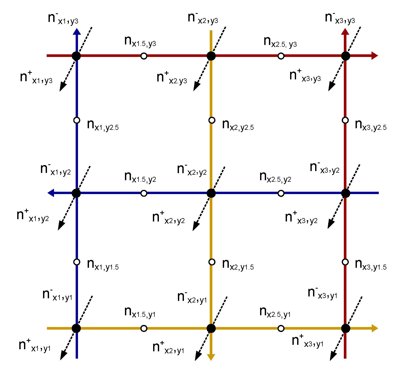
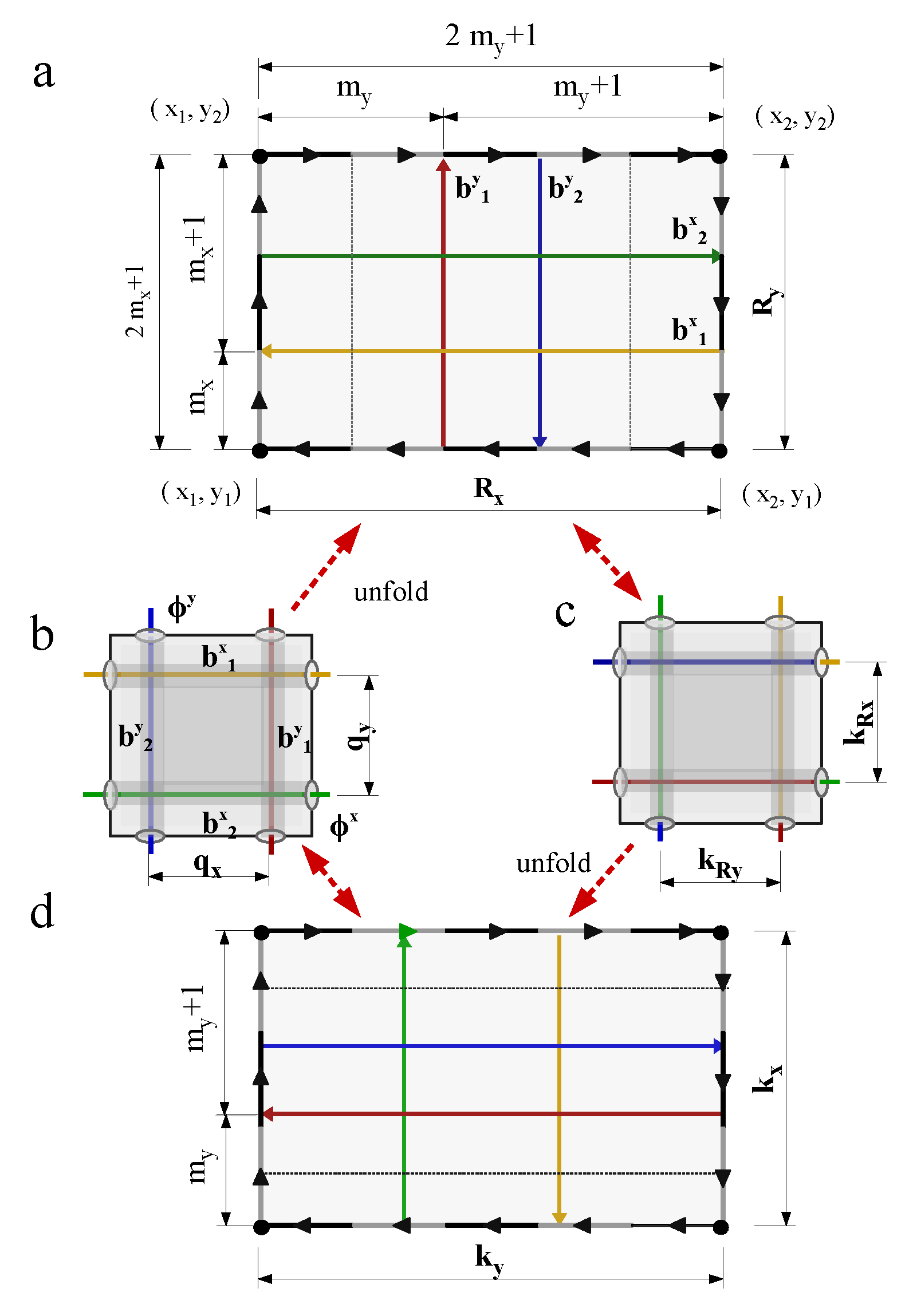
Figure 46.
The number of laminar layers around three magnetic fluxes in axis that over-crossing( or under-crossing) three magnetic fluxes in axis are labelled at the crossing points. The number of bonding laminations are labelled one the bonds of the square knot lattice.
Figure 46.
The number of laminar layers around three magnetic fluxes in axis that over-crossing( or under-crossing) three magnetic fluxes in axis are labelled at the crossing points. The number of bonding laminations are labelled one the bonds of the square knot lattice.
Figure 47.
(a) The unfolded lamination generated by braiding two perpendicular flux pairs in opposite chirality to that for generating the folded lamination in (b). (c) The folded lamination is summarized into two perpendicular bond carrying fractional fluxes. (d) The square lattice of fractional fluxes is generated by translating the unit cell in (c).
2.10. Fractional Hall conductance quantized by Chern number of folded lamination in three dimensions
The electron fluid lamination in homogeneous magnetic field is quantum fluid that obeys Schrdinger equation. The magnetic fluxes in certain direction are all parallel to one another, folding the electron fluid monolayer into stacked flat laminations without buckling or concave (as showed in Figure 47b). When the unit cell in Figure 47b translates to fully cover a homogeneous square lattice of magnetic fluxes oriented in two perpendicular directions, the periodic electron fluid confined in x-y plane is described by a magnetic Bloch wave function ,
where the potential is a periodic function in Schrdinger equation above, is the unit lattice space between two nearest neighboring fluxes. The Bloch wave functions satisfy . The four magnetic field lines around an unit square cell of unfolded lamination in Figure 47b confines one x-flux and one y-flux, since each flux line segment is shared by two nearest neighboring unit cells. The Hamiltonian is invariant under magnetic translations [37],
Here the magnetic translation operator () characterize the periodic distribution of magnetic flux lines oriented in x-axis (y-axis).The magnetic translation operators commute with Hamiltonian .
Without losing generality, we first fold one unit cell in real space (the whole grey rectangular zone in Figure 47a) by times of parallel braidings on x-flux pair (y-flux pair), to generate a highly folded unit cell of lamination in Figure 47b. The unit cell lamination in Figure 47b is overlapped by layers of stacked monolayers. Every monolayer within the unit cell lamination confines a pair of fractional flux quanta,
The square grid of perpendicular magnetic fluxes in plane can be generated by choosing generalized Landau gauge . Unfolding this heavily stacked unit cell lamination into a square array of many unit square monolayers in Figure 47a extends the original unit lattice space to
The oscillating pattern of electron fluid lamination in the square grid is collective wave formed by intersecting plane wave two dimensions with lattice spacing and . Because every unit square monolayer in Figure 47a carries a fractional flux quanta defined by Eq. (272), the two magnetic translation operators along are not commutable,
where the fractional flux within unit square monolayer of Figure 47a is quantified by the product of two independent filling factors,
The magnetic translation operators over an enlarged unit square consists of unit square monolayers are commutable,
because the extended unit cell confined by and contains two integral flux quanta , guaranteeing the commutation relation . The corresponding Bloch wave function on the periodic lattice of extended unit cells reads
The folding (or unfolding) operation in momentum space is exactly the inverse operation of that in real space. Folding the unit cell in real space leads to the unfolding of Brillouin zone in momentum space, because the absolute magnitude of reciprocal unit lattice vector is proportional to the inverse of unit lattice vector in real space. The reciprocal lattice space with respect to the unit cell in real space of Figure 47a reads
which fulfills the reciprocal relation, . When the large unit cell in Figure 47a folds into a small unit cell with stacked lamination in Figure 47b, the reciprocal unit cell lamination defined by in momentum space is unfolded and expanded into a large reciprocal unit cell defined by , covering small reciprocal unit cells of the original size . The inverse operation of unfolding the unit cell of stacked lamination in Figure 47b into Figure 47a compresses the Brillouin zone with momentum vectors ) into a smaller Brillouin zone with .
The folding (or unfolding) operation of electron fluid surface is controlled by the effective magnetic field strength. A reduction of magnetic field strength results in corresponding increment on stack number of monolayers around the flux pair. On the contrary case, the stack number of monolayers is reduced with respect to an increasing magnetic field strength. Since folding (or unfolding) operation in real space results in exactly opposite topological effect to that in momentum space, the effective magnetic field strength in real space is the inverse of that in momentum space, i.e.,
In real space, the two fluxes in the same direction are placed in opposite domains of three dimensional space divided by the two dimensional electron fluid surface. Each of the unit squares covering the unit cell in real space carries a fractional flux , indicating a decreasing magnetic field strength as and grows. In the meantime, the unit square monolayer of Brillouin zone in momentum space folds into stacked unit lamination with monolayers, resulting in an increasing magnetic field strength in momentum space as and grows. The Bloch band denoted by energy curves in unit cells of momentum space correspondingly splits into stacked sub-bands in unit lamination of stacked Brillouin zones. The two perpendicular flux pairs divide the unit cell in real space into four sub-unit cells carrying four pairs of fractional fluxes respectively (Figure 47a),
The sum of fractional fluxes in the same side of the electron fluid surface equals to two integral flux quanta, . The () layers of monolayers above the magnetic fluxes and (denoted by the yellow and red bold lines in Figure 47a) generates fractional fluxes,
which locate at the horizontal and vertical bonds respectively in the folded unit cell (Figure 47b-c). The two perpendicular flux pairs approaches to the middle lines of the rectangle when , dividing the unit cell into four equal sub-unit cells filled by half flux quanta .
When the square lattice composed of many uniform fractional flux pairs is folded back to the unit cell with two integral fluxes in Figure 47b, the collective state of electron fluid on the lattice of integral fluxes is described by magnetic Bloch state, which is a complex fibre bundle on base manifold of magnetic Brillouin zone,
The Hall current driven by external electric field is derived by linear response theory [22],
where the current operator is defined by the quantum momentum operator, . The Hall current Eq.(283) is reformulated into a brief commutator form
by renormalizing the two currents with energy gaps
The Hall conductance tensor is the coefficient of electric current in response of external electric field, ,
which is exactly the familiar Berry curvature of magnetic Bloch states
which characterize the topology of the magnetic Brillouin zone, leading to a topologically quantized Hall conductivity by the first Chern number n of the magnetic Brillouin zone [22],
The Chern number n is an integer in the magnetic Brillouin zone confined by .
When the stacked unit cell in Figure 47b is unfolded and expanded to a square lattice composed of many uniform fractional flux pairs , the electrons hopping from one site to another in the unfolded square lattice gain fractional phases. Both the magnetic Bloch waves and magnetic Brillouin zone are squeezed into small Brillouin zone, however the Chern number is independent of this scale transformation,
whose value is exactly equal to the topological number in Eq. (288). The area of Brillouin zone of the unfolded square lattice is times of the stacked unit cell, i.e.,
Eventhough chiral braiding operation does not change the topology of Brillouin zone, but can split the magnetic Bloch waves into different propagation modes with opposite chirality. The unfolded square lattice are covered by chiral fractional fluxes , which are defined by its location to the left (or right) hand side of the fluxes in Figure 47. There are Brillouin zones to the left hand side of flux and to the right hand side of . The chiral edge states running along the edges of the two dimensional space only occupy the unit cells with the same chirality in the unfolded square lattice. As a result, the Chern number of whole Brillouin zone is decomposed into different fractions with respect to different chiral subzones,
The quantum Hall conductance is quantized by fractional topological numbers,
The fractional filling factors is determined by braiding string operator. For the square lattice of chiral fractional fluxes in Figure 47, the fractional Hall conductance explicitly reads
where is the braiding period number in -axis.
The eigenenergy with respect to certain fractional Hall conductance can be derived from Harper equation [34]. The collective wave function of the folded electron fluid lamination obeys two dimensional discrete Schrdinger equation,
which is a generalization of the discrete Harper equation for electrons immersed in homogeneous magnetic field in z-axis [34]. Here the effective magnetic field strength B is quantified by the inverse of fractional filling factor , i.e., . Then the discrete Harper equation with respect to fractional quantum Hall states with reads
The train track generated by a pair of antiparallel fluxes always leads to a rational filling factor, . The wavelength of the oscillating lamination can exactly overlap an integral number of the lattice space between the two fluxes within one pair, generating a stable standing wave pattern crossing the unfolded lamination plane. The fractal energy spectrum of Hofstadter butterfly[35] reduced to a collection of pure fractional Hall fluid states, which matches knotted orbital in phase space [12].
The Berry curvature acts as an effective magnetic field, attracting an electron to circle around a local extremal point of curvature in momentum space [37],
where is an uniform electric field. The tensor equation of motion for electron in three dimensional electric field is
A closed orbit of a moving electron in real space corresponds to a rescaled closed orbit in momentum space that is rotated by . The physical effect of curvature tensor is equivalent to an effective magnetic field in momentum space, generated by symmetric gauge potential vectors in three perpendicular directions,
The effective Hamiltonian for Schrdinger equation in three dimensional magnetic field is
where is effective mass of electron in lattice. The covariant derivative operators are
The Berry curvature in three dimensional momentum space is quantized by the Chern number of curvature tensor in an unfolded three dimensional reciprocal lattice with respect to the folded unit cell in real space,
When the two dimensional unit cell confined by are folded into stacked unit lamination defined by , the three dimensional Brillouin zone expands to a large Brillouin zone with reciprocal unit lattice spaces
A train track in real space is also mapped into a rescaled train track in momentum space. The train track pattern in the cross sectional plane perpendicular to fluxes in x-axis (and y-axis) defines a chiral fractional flux (and ) and fractional unit lattice space,
The fractional quantum Hall conductivity with respect to train tracks in (and ) plane is (and ),
The fractional Hall conductance tensor above coincides with the Hall conductance coefficient derived from the classical Drude model in three magnetic field (See Appendix A), which also predicts the diagonal resistivity .
2.11. The collective wave function of 3D fractional quantum Hall states represented by quaternions
If the magnetic fluxes are all located on the same side of the laminar surface, no matter how many times the fluxes lines exchange, the laminar surface is not really folded and can always restore its original unfolded configuration. Therefore the magnetic fluxes split into two separated sets in the simply connected space that is divided by the laminar surface. The plane of two dimensional knot lattice could be oriented to be parallel to the laminar surface. Once a flux that is perpendicular to the laminar surface is introduce to the two dimensional knot lattice, it inevitably penetrates through the laminar surface, driving the electron fluid to flow around itself in a helical path, until a worm hole is finally formed to connect two separated laminar surfaces (the blue surface and red surface in Figure 48a). Many fluxes are topologically equivalent to many genus of a continuous manyfold (Figure 48a). In fact, electron fluid lamination can also construct multiply connected surfaces that envelopes the two dimensional lattice completely (Figure 48b). In that case, even if all magnetic fluxes are locked inside the multiply connected surface, braiding magnetic fluxes in parallel still generates non-trivial folding, which demonstrates the same train track pattern as bare flux knot lattice. The multiply connected surface that envelopes three dimensional knot lattice is generated by cutting two holes at the north pole and south pole of the sphere centered at a crossing point (Figure 48c), with the equatorial plane overlaping with the plane of two dimensional knot lattice. Three mutually perpendicular fluxes overcross (or undercross) at this crossing point, constructing different local knot configurations. All possible crossing states can be characterized by the relative location vector of projecting the other two fluxes along two different axis to certain flux along the third axis [12],
The normalized vector is Ising spin in three dimensions. Besides the eight different crossing states, there are still many vacuum states composed of self-avoiding flux arcs connecting the face centers at different axis and many hybrid states with two vacuum arcs and one crossing flux [12].
Here we introduce Hamilton quaternion to characterize a general crossing state of three magnetic fluxes in knot lattice. As showed in Figure 48c, a general magnetic flux vector is expanded by quaternion basis ,
where , and , , . is an unit number. The Pauli matrices for spin is a natural matrix representation of quaternion, , , . This quaternion flux vector exactly characterizes the spin Eq. (304) due to the anti-commute relations,
The quaternion representation of the vacuum state composed of vortex arc pair and a straight flux line has a similar formulation as following
The full vacuum state composed of three vortex arcs has the following form,
Exchanging the locations of two fluxes maps an over-crossing state to an under-crossing state (or vice versa), flipping a local spin from S to . In Figure 48c, all magnetic fluxes are fully enveloped within the multiply connected electron fluid surface, braiding fluxes does not change the topology of the laminar surface. Therefore the fractional quantum Hall states in the cross section of the multiply connected laminar surface still matches the abelian Chern-Simons field theory, which is described by the effective wavefunction of Wen-Zee matrix formulation [17].
When the electric tubular surfaces that envelope magnetic fluxes in different axis avoid intersecting with one another, as showed in Figure 48d, the highly degenerated collective Hall states in three dimensions split into many sub-states which is characterized by crossing states of flux knot lattice. The surface state on the boundary surfaces of finite three dimensional knot lattice is fractional quantum Hall state. When the flux tubes are braided in parallel, the boundary state is identical to any cross-sectional state in the bulk. Figure 48e showed the stacked lamination after braiding two fluxes in parallel that belong to two separated enveloping tubular surfaces once, the train track pattern on the top and bottom plane corresponds to fractional charge states . m times of braiding operations leads to the fractional filling states () on the top and bottom boundaries. Parallel braiding is physically implementable by homogeneous magnetic field strength in three perpendicular directions. The fractional states around the eight corners of the cubic knot lattice obey non-abelian statistics [12]. The abelian Chern-Simons field theory is inadequate to describe the electron fluid flowing along the tubular surfaces in knot lattice, the non-abelian Chern-Simons field theory has to be introduced to establish an effective topological field theory [15] for the 3D knot lattice of quantum Hall fluid,
where is the gauge field potential in the tubular surface, and is expanded by the generators of group (i.e., ).The hierarchy construction of abelian Chern-Simons Lagrangian for fractional quantum Hall state is extended to non-abelian Chern-Simons theory in a straightforward way,
The Wen-Zee wavefunction for abelian quantum Hall states is constructed in complex plane with locations of electron denoted by complex number [17]. In mind of the exact correspondence between quaternion and Pauli matrices, the spatial locations of electrons in three dimensional knot lattice of electric tubular surface can be denoted by quaternions,
In order to construct the wavefunction in three dimensions, the complex variable of locations is extended to quaternions. The effective collective wavefunction with respect to non-abelian Chern-Simons theory is generalized as
In abelian Chern-Simons theory for fractional quantum Hall states, the filling factor Eq. (79) equivalently maps the fractional filling factor constructed by Wen-Zee formulation into a fraction of linking number of magnetic flux knot lattice. The topological quantum field theory suggested that non-abelian Chern-Simons action is also a topological invariant of link [15]. The topological linking number of a three dimensional knot lattice is directly countable by projecting every crossing point of three mutually perpendicular tubes into the same two dimensional plane, the projected locations of crossing points must be carefully arranged to avoid overlapping. Figure 48f showed an exemplar projection of crossing point in three dimensions into a knot configuration in two dimensional plane, which has a linking number Every local crossing point is characterized by an unique spin state, , which has one-to-one correspondence with linking number . Thus the total linking number of the knot lattice is the sum of all local crossing states, . The total linking number is invariant with respect to an eigenstate. The knot lattice configuration of electron fluid tubes can be reconstructed under thermal fluctuations. The partition function of all possible knot lattice configurations is a topological invariant.
The effective collective wavefunction Eq. (312) determines the spatial probability distribution of an electron within certain branch of train tracks
where and . This probability distribution is reformulated into a Boltzman distribution form by introducing an analogue potential . Similar to the partition function in statistical physics, the analogue partition function for many electrons is effectively defined by the product of probability distribution of all electrons confined in the train track pattern
The analogue potential of Hall fluid has a similar form of harmonic oscillator potential
, the first two terms at the right hand side of Eq. (315) summarizes the interaction between parallel electric current segments within a stacked train track pattern, while the third term is a parabola potential well that generates quantized energy levels with equal energy gap, which reflected the physical effect of a homogeneous magnetic field. The effective potential surface deformed into a hyperbolic surface when the electron approaches to the edge.
The locations of electron flowing in the tubular knot lattice is expressed by Pauli matrices to encode the non-abelian nature of three dimensional knot lattice,
The interaction potential between two parallel electric currents and parabola potential well are spontaneously constructed within this non-commutative space,
The coefficients in front of are collected and summarized into a function to derive a compact formulation of analogue potential for Hall fluid in three dimensions,
This potential is consistent with the non-abelian Chern-Simon action Eq. (309), which transforms into similar form as Eq. (318). The analogue potential regrouped the energy levels into two energy bands,
The energy gap between two bands is finite in the bulk, but drops to zero on the edge,
The landscape of effective potential for fractional quantum Hall effect in Figure 30 is a qualitative visualization of the analogue potential . In real space, the energy gap closes when the incompressible lamination is penetrated through by magnetic flux lines perpendicular to the folding plane of lamination. Every gap closing point, locating at the solution of , is characterized by a topological winding number, that counts how many times the unit vectors winds around the origin point,
Duan’s topological current theorem [21] suggests that the sum of these local winding numbers equals to the first Chern number of base manifold,
where is Dirac function, is the winding number around the ith energy gap closing point of . is the Jacobian of vectorial energy space in real space. The topological vortices locate at the solution of . There are m energy gaps closed on the edge with respect to fractional filling factor , with the energy gap ruled by the energy Eq. (198).
The Chern number is an integer as the sum of winding numbers of all singular points, either circling around by clockwise flows or counterclockwise flows, it is independent of the chirality of circling motion around singular points. However, the action of magnetic field breaks time reversal symmetry, only the circling flows with the same fixed chirality are allowed to transport along the edge, the edge flow with opposite chirality are eliminated out of conductivity measurement. The gapless points on the left (right) edge are denoted as (), the complete Chern number is the sum of the chiral winding numbers,
The viscous electron flow can only passes one of the two edges in FQHE due to the far distance between them, the measurable chiral Chern number on edge is a fraction of the whole Chern number,
where is a polynomial of the chiral filling factors. When the transformation operation between different knot states in three dimensional knot lattice are taken into account [11], the fractional Hall conductivity are quantized by the second Chern number as well as higher order Chern numbers.
The knot lattice of magnetic fluxes generates non-abelian magnetic field in three dimensions. We choose a special symmetric gauge potentials along the knot of magnetic flux tubes and expanded it by quaternions,
The effective magnetic field with respect to the gauge potential vector above reads , which is replaced by non-abelian gauge field tensor in knot lattice,
The abelian magnetic field corresponds to the gauge field tensor ,
The first term on the right hand side of Eq. (327) represents the abelian magnetic field, which reduces to in the absence of quaternion representation of knot. The rest three terms represents the non-commutative character magnetic fluxes in knot lattice. The magnetic field in z-axis is influenced by the product of . The magnetic fields in the other two directions both join in the gauge field tensor. The highly entangled magnetic field components results in complex relation between Hall resistivity and magnetic field. The current tracks form closed loops under periodical boundary condition. The gauge field tensor alone these loop tracks is periodical function, which transform into brief formulation under Fourier transformation,
The Hall conductance tensor in the chiral Brillouin zone is fractional number determined by laminar folding of momentum space,
The fractional Hall conductance tensor in three dimensional knot lattice of magnetic fluxes includes nonlinear terms denoted by the product of four fractions. These higher order contribution is much smaller than the dominant fractional terms denoted by the product of two fractions in Eq. (329), which is also much smaller than the Hall conductance in two dimensions, because the contacting area between viscous laminations is much larger than that between viscous paths in two dimensions. Therefore the fractional Hall conductance in three dimensions hard to detect. More over, the non-abelian fractional Hall conductance tensor can be extended to four dimensional space time, where the Hall conductance is quantized by the second Chern number. The fractional Hall conductance in four dimensions is composed of product terms of eight fractions. Viscous electron flow swirls around a singular time line in curved space time. The three dimensional fractional filling factors predicted here is testable by quantum Hall system in a tilted magnetic field, which is well developed both in theory [38] and experiment.
3. Topological representation of anyon in three dimensions by folded multilayer laminations
Indistinguishable particles are classified into two fundamental types, fermions and boson. Fermion has half integral spin , while boson has integral spin , where m is integer. The collective wavefunction of two interacting fermions is antisymmetric, which is expressed as a complex function of the locations of the two fermions and ,
While the collective wave function of two bosons is symmetric function, i.e., If the exchanging of two quantum particles contributes a non-trivial phase to the collective wavefunction,
These quantum particles are classified as anyon [8] with an effective spin The statistical phase in Eq. (331) is independent of the distance between the two particles . Exchanging the locations of two particles indicates an exact closed loop formed by the trajectories of the two particles, any small deviation from the original location points breaks the closed closed loop into an open path. The statistical phase is determined by the topology of the trajectory loop of one particle around another.
The spatial ordering of many interacting particles is a topological ordering independent of the relative distances among them. In Figure 49a, the point particle locates in the inside domain enveloped by a circular boundary B, where the outside domain is filled by the second point particle with its center labeled by . The boundary between the two particles is the coexistence domain created the product of . The boundary is assigned with a phase factor and vanishes if either one of the two particle annihilates. The statistical phase defines a phase gradient vector pointing from to . When particle crossed the boundary into the outside domain, it gains or losses a phase difference to join the same domain as , where the boundary between the two particles vanishes, transforming the two fermions into two bosons. The particle surrounded by an odd number of circling boundaries is fermion. Every particle is represented by a singular point in a topological domain, if there is no singular point existing in the domain sandwiched in between two nearest neighboring boundaries, the two boundaries fuse into one by continuous topological contraction.
In Figure 49b, a quantum state is represented by a compact two dimensional manifold. A fermions with spin is a singular point surrounded by a circling boundary. The outer domain outside the circular boundary can be filled by another fermion with spin , which corresponds to a domain enveloped by a boundary circling in opposite chirality. A third particle either inside the circle or outside the circle is forbidden due to the violation of statistical rule of fermion that is only allowed to have an odd number of boundaries. Three quantum states are represented by three compact manifolds, at most two singular points are allowed to occupy one quantum manifold, visualizing an exact topological representation of Pauli exclusion principal. In Figure 49c, singular point enveloped by only one circular boundary can coexist with another one within the same quantum manifold of , because there are two layers of boundaries between them. More singular points enveloped by one circular boundary can coexist within the same quantum manifold of , since there are two layers of boundaries among any two singular points. This topological representation exactly visualizes the statistical character of many interacting bosons.
The boundary line segment in Figure 49 is expanded to a cylindrical manifold to construct an unified topological representation of fermion, boson and anyons. When the fermionic fluid around the singular point flows over half of the cylindrical boundary, its phase continuously reduces until it meets the fluid in the other domain around . The front line of the fermionic fluid around sweeps over along the circular cross section of the cylindrical boundary with infinitesimal radius in Figure 49ab. When the quantum fluid filled with domain rotates around the cylindrical boundary over an angle of in Figure 49cd, the quantum fluid in domain gains a phase of to meet anyonic quantum fluid in . For bosonic quantum fluid in Figure 49ef, the topological fluid sweeps over either zero phase or to meet topological fluid . The intersecting lines between the cylindrical boundary and fluid surface determines the statistical phase of two coexisting fluids on boundary. The statistical phase is a topological factor, because it is independent of the curvature of the cylinder.
The fractional statistical phase of anyon in FQHE is generated by braiding two fluxes separated by an electron path. In Figure 51a, the magnetic fluxes are represented by two singular points in two opposite sides of the boundary line. A clockwise braiding of the two singular points generates the spiral boundary pattern with respect to . The single boundary line between two singular points folds into three layers of stacked boundary line (In Figure 51b). The three layers of boundary segments share a phase of to keep the continuity of phase field. Each of the three stacked boundary segments carries a phase . The particle must cross two layers of boundary to enter its original region on the left hand side, gaining a phase . However has to travel another distance of to reach its original location, it losses another phase factor (In Figure 51c). In the end, the statistical phase of point particle is .
When the two particles are braided in counterclockwise direction in Figure 51d, the first period of braiding exchanges the mirror locations of the two particles in opposite side of the boundary mirror. The second period of braiding brings the two particle to their original locations and fold the boundary into a triple layer boundary (Figure 51e). Both the two particles have to cross two layers of boundary lines to return to their original location points (Figure 51f), gaining a statistical phase of ,
Therefore braiding particles divided by non-trivial phase boundary renormalized the monophase boundary as mixed phase boundary, driving the conventual statistical phase of fermion or boson into fractional phase of anyons. The phase mixing effect changes the relative statistical phase of all particles to the two particles that take part in the braiding operation, no matter how far they are separated. The four particles in Figure 51g are grouped into three different domains, is in the green zone, in the white zone, while and are in the gray zone. Braiding and bridges them with four layers of boundary lines, where single layer carries a fractional phase . The left hand and the right hand side of are covered by three layers and one layer of boundary line respectively (Figure 51h). The phase around are divided into four equal fractional phases, . The relative phase between and is . The phase difference between and is . The phase difference between and is . and are initially bosons with a statistical phase , the clockwise braiding transforms them into fermions with statistical phase of . The fermion pair and transform into anyon pair.
The statistical character of interacting quantum particles in three dimensions can be represented by two dimensional boundary surfaces. In Figure 52a, the boundary surface with a phase divided the three dimensional space into two fermionic domains, each of them is filled with fermionic quantum fluid. Two interacting point particles in three dimensional solid ball are divided by a two dimensional surface into two separated domains in Figure 52b. When the blue particle winds around the red particle and returns to its initial location, a fermionic blue particle would gain a phase factor , while a bosonic blue particle gains a phase . The closed path in Figure 52c shrinks to the initial location point by continuous topological contraction. In this case, the statistical phase of two interacting particles is either or , i.e., the particle is either boson or fermion, anyon does not exist in this space. When the three dimensional space is divided by a torus surface with one genus in Figure 52d, the winding path in a simply connected region still contracts to a point continuously (the green loop in Figure 52d), however the winding path passing the multiply connected region cannot contract to a point due to the unavoidable genus on its way (the blue loop in Figure 52d). In a multiply connected region with two genus, the closed path of a particle could winds into different knots, leading to non-trivial statistical phase of two interacting particles, with statistical phase , where is the winding number around the ith genus. However here the two point particles are either fermion or boson, because the point particle did not penetrate through the boundary surface to enter the other domain.
When two fermions are separated into opposite domains divided by two dimensional boundary surface, braiding the two fermions in three dimensions traps them by highly folded boundary surface. The stacked laminar surfaces fuse into one renormalized boundary surface due to quantum interference. The fermion has to cross a number of boundary layers to return its initial location. The the two interacting fermions transform into two interacting anyons in three dimensions. In Figure 53a, the two fermions (denoted by the blue dot) and (denoted by the red dot) are in the front and the back domains respectively. The upper edge of boundary surface bends toward the front domain to wrap around the fermion . The bottom edge bends into the back domain to envelop the fermion (Figure 53b). In Figure 53c, the horizontally folded boundary surface is further folded around a vertical axis. The resultant laminar boundary surface forms nine layers of stacked boundary surfaces that traps the two particles. There are five (four) layers above () and four (five) layers below () in Figure 53c. The statistical phase of the two particles and is ,
For a general case of periods of braiding in x-axis followed by periods of braiding in y-axis, the boundary surface is a lamination consisted of monolayers. The number of monolayers above the particle is , while that below is . and form a pair of anyons with fractional statistical phase,
The fractional phase serial converges to when and grow from 0 to infinity. Either or reproduces the fractional serial of anyons in two dimensions. For , the fractional numbers are much less than that of two dimensional case and converges quickly to . The laminar boundary surface can be implemented by viscous electron fluid. The two particles are simulated by either singular points in three dimensions or effective magnetic monopoles in frustrate spin ice.
Singular loop in two dimensions is equivalent a point particle represented by a singular point, showing the same anyon statistics under braiding operation of many loops, but experiences much more complex collision phenomena than point anyons, because the point-like anyon in this case has topological internal structure. A singular loop is either a topological ring defect in liquid crystal or a magnetic flux loop immersed in two dimensional electron fluid. A simple connected region in Figure 54a can be viewed as vacuum state. Two new loop boundaries (the blue loop and red loop in Figure 54b) are created simultaneously by the cutting action on vacuum states. The antisymmetric wave function of the two loop boundaries are denoted as
where denotes the radius of the loop boundary. The two loop anyons are separated by a singular gap that divides a simply connected region into two separated regions (Figure 54a). This singular gap zone is the boundary surface between two loop particles and carries a statistical phase . Unlike two point particles, two loops interlock with each other to move together as a pair in two dimensions. There is no physically implementable path for two loops exchanging their locations unless there is a tunnel through the loop gap to fuse two loops into one ( Figure 54c). After the blue fluid and red fluid in Figure 54a exchanged their locations, withdrawing the tunnel restores the interlocking two loops. The singular loop gap between two loop shrinks to a singular point due to the existence of tunnel. In three dimensional solid ball, the inner sphere surface and the outer sphere surface are also generated by pairs under cutting action along a boundary sphere in Figure 54b. The tubular tunnel surface fuses the inner and outer sphere into one big sphere. The blue outer sphere deforms into a concave sphere to replace the original red sphere (Fig. Figure 54c). Two tubular tunnels transform the two separated sphere into a torus with one genus, exchanging of the original two boundary spheres is realized by rotating the torus sphere around its radial central circle (Fig. Figure 54d). More over, four tubular tunnels fuse the two boundary spheres into a torus with three genus (Fig. Figure 54e).
Magnetic loop interlocking with electric loop is a natural solution of Maxwell equation of electromagnetic dynamics. When the constant magnetic loops are immersed in viscous electron fluid, the electron fluid lamination flow around the magnetic loop to form torus laminations. Figure 55b showed four layers of concentric torus divided by four magnetic loops. If all of the four magnetic loops are braided rigorously in parallel, i.e., all points of one magnetic loop move simultaneously in the same way, the vertical cross section of the lamination torus corresponds exactly to anyons in two dimensional viscous fluid of FQHE. Here the cross section of electron fluid torus is the closed path of electron flow. The cross section point of the magnetic loop is the singular point of magnetic fluxes in FQHE. Each electron fluid loop in cross section plane is represented by a fermion operator, the interlocking four loops are denoted by the product of four fermion operators, , because they have to move together as a quadramer in space (Figure 55b).
When the magnetic loop is cut into two semicircular arcs, four contacting points are created on the left and the right cross section, and (Figure 55a). If the contact points of the four magnetic flux loops in different cross sections are not braided following the same protocol (Figure 55b), the magnetic fluxes form nontrivial knot lattice pattern (Figure 55c-d-e). In Figure 55bd, the flux No. 1 and No. 2 in the right cross section are braided once in clockwise direction, because flux No. 1 together with its torus envelope are in the same domain as bare flux No. 2, there is no fractional charge generated in this braiding. Flux No. 1 and No. 2 in can reconnect to the corresponding contacting points in by keeping the topology of torus surface around them invariant. In Figure 55d, the flux No. 3 and No. 4 are braided in clockwise direction, mixed two opposite domains that holds flux No. 3 and No. 4 respectively. In Figure 55e, two clockwise braiding on flux No. 3 and No. 4 folds the boarder surface into a lamination with four layers. An integral charge splits into and when it passes flux No. 3. Because the cross section of the torus surface in is not folded, it cannot reconnects to the train track which is the cross section of torus surface around flux No. 3 in without introducing new genus to the torus surface. The flux No. 4 in has to penetrate through the surface twice to connect to flux No. 4 in in Figure 55e. This penetration creates two topological vortices on the electron fluid torus surface. Another equivalent way of creating the two topological vortices is to keep the boarder surface flat and to braid the flux No. 3 and No. 4 into either overcrossing state or undercrossing state. If the initial position of flux No. 3 (No. 4) is below (above) the boarder surface, the open ending points of the two fluxes bend within the same domain to create an overcrossing state of flux No. 4 over flux No. 3. A further braiding in the same direction leads the two flux lines into an inevitable penetrating through the boarder, creating at least one hole in the boarder surface. Electron fluid swirling around this singular hole forms topological vortex.
4. The topological representation of chiral spin liquid by knot lattice
4.1. Topological representation of chiral spin liquid in one dimensional ring of knot lattice
A classical spin of electron is equivalent to magnetic dipole that generates the same magnetic momentum . In Figure 56, the classical is depicted as a solid bar with its two endings attached by two magnetic monopoles of opposite charges, the black dot (the unfilled circle) has positive (negative) charge. The nearest neighboring spins prefer forming antiferromagnetic order due to the attractive interaction between magnetic monopoles with opposite charge. In a weak magnetic field, some spins are aligned to the direction of external magnetic field under thermal fluctuations. The spin chain along a ring of Figure 56a is modeled as a classical Heisenberg spin chain, where the spin is represented as a two dimensional vector in the plane that confines the radius R and z-axis, where is the deviation angle of a spin from z-axis at the ith site (Figure 56b). The Heisenberg Hamiltonian
describes the superposition of waves that depends on the phase difference between nearest neighboring spins
where the phase difference equals to the gradient of phase field in continuous limit, . If a spin deviates a large angle from local minimal point, the cosine function of interaction cannot be approximated by parabola, instead it is cosine wave pattern. The interaction between two spins with large deviation is approximated by Taylor expansion up to the fourth order,
The antiferromagnetic spin chain is equivalently represented by two parallel neutral loops that connect alternating magnetic monopoles( the blue and yellow dashed loop in Figure 56a). Flipping the spin to align it with and in the same direction, raise the minimal energy point up to a local maximal potential energy at in Figure 56b, due to the repulsive interaction between magnetic monopoles. (Figure 56a) prefers rotating to reach one of the two degenerated minimal energy states in Figure 56c. The topological ribbon sandwiched in between two parallel neutral loops is formed by high density electron fluid, the strong attractive interaction between magnetic monopoles of opposite charges keeps the continuity of the two edge loops. If rotates further more than , the continuous edge loops drag the next nearest neighboring spins to deviate from their local minimal energy states, raising up the potential energy in vicinity of . The potential energy around a local spin shares the same landscape with the well-known model in classical field theory in Figure 56c.
The one dimensional knot lattice is essentially an one dimensional lattice of topological solitons that fulfills the classical model. The accumulating phase field describes the basic character knot crossings, denotes the phase of a spin deviating from the z-axis, s is the distance to the initial point of the spin. Every crossing in knot lattice is equivalent to a kink excitation. The dynamics of knot crossing is described by the Lagrangian,
A local crossing state of knot lattice fulfills the topological kink excitation,
The overcrossing state (or undercrossing state) corresponds to kink(or anti-kink) respectively. The energy density of knot crossing is
Both the overcrossing and undercrossings have the same energy density localized at site , acting as a topological soliton.
Two interlocking magnetic lines wind around each other to create more crossings under thermal fluctuation. The crossings are topological solitons that are always created or annihilated by pairs. The total energy of solitons in knot lattice is proportional to the total number of solitons despite of the sign of their topological charges.
where is the initial total number of crossings. The number of solitons in ground state is a topological number protected by the topology of alternating knot ring, because a local soliton cannot be annihilated unless the topology of the knot lattice suddenly changes. The total number of spins in a spin chain is conserved for both periodical and open boundary condition. While the total number of crossings in knot lattice is not conserved, because new crossings are excited up by external input energy. The sum of signs of all crossings in a ring of alternating knots is twice of topological linking number. A local flipping of spin creates or annihilates two opposite crossings simultaneously, keeping the linking number invariant but transforming the initial antiferromagnetic spin ordering into a spin liquid state at higher energy level. Flipping local crossings at different lattice sites creates different spin liquid states. The degeneracy degree of spin liquid state with energy is
These spin liquid states share the same topological linking number as the initial alternating knot ring as long as the topology of knot ring is kept invariant.
The Jones polynomial remains the same form at different temperatures as long as the alternating knot ring keeps its original topology under thermal fluctuations. The Jones polynomial not only characterize the topology of the knot lattice with crossings, but also encoded the topological transformation process of a zero crossing state growing up crossings step by step. All different growing paths lead to the same Jones polynomial. A local crossing in knot lattice is unstable at high temperature and oscillating between opposite crossing states (, ). The alternating knot ring is formed by one circle for an odd number of crossings (Figure 56d). For an even number of crossings, the alternating knot ring is generated by two intertwined magnetic loops (the blue loop and yellow loop in Figure 56e). Flipping a crossing to crossing reduced the total number of crossings from to (Figure 56f).
The one dimensional ring of interacting particles mapped into a torus with magnetic current lines winding around the surface of torus. Winding the magnetic current line through the genus of a torus p times and q revolutions around the central ring to glue to its initial point generates a torus knot showed in Figure 56d-e-f. The integer (or ) counts the total number of chiral crossings. The Jones polynomial of a torus knot reads [18]
where t is Boltzmann weight factor The torus knot is exactly the familiar trefoil knot. The topologically invariant probability of torus knot ring consists of left-handed crossings is characterized by Jones polynomial
The von Neumman entropy of the torus knot measure all the probability distribution of all possible loop states generated out of the knot ring,
Figure 57 showed the von Neumman entropy of torus knot composed of the right-hand crossings and the left-hand crossings. The entropy decay exhibits distinct evolutionary curves for different chirality of the torus knot. The torus knot, consisting of right-handed (or left-handed) crossings, decays to zero at zero temperature (or finite temperature). This decay curve of entropy agrees with that observed for the trefoil knot in Figure 10. The von Neumann entropy, , corresponding to different chirality of the torus knot, diverges into distinct branches at low, intermediate, and high temperature zones. At low temperatures, such as shown in Figure 58, the entropy of the left-handed torus knot is zero, whereas the entropy of the right-handed torus knot, , initially peaks at before decaying to zero for . At an intermediate temperature of (Figure 59), the von Neumann entropy, , of the left-handed torus knot initially reaches a maximum at and subsequently declines to zero for . Conversely, the entropy of the right-handed torus knot, , gradually increases to a maximum at and then slowly decreases as p increases. At a high temperature of (Figure 60), the entropy of both the left- and right-handed torus knots increases monotonically with p, although the rate of increase for the left-handed knot consistently exceeds that of the right-handed knot. The absence of entropy at low temperatures indicates a highly ordered topological phase, while the increase in entropy at high temperatures results from a disordered phase induced by thermal fluctuations.
4.2. chiral spin liquid in two dimensional knot lattice
A conventional spin is represented by a rotating quantum droplet, which carries the same mass, electric charge and momentum of a conventional electron. The droplet deforms into different shapes following the Schrdinger equation, with its density distribution matching exactly the electron wavefunction. An electron gas of many free electrons is represented by many isolated droplets. An electron fluid is represented by many droplets (the green discs in Figure 61a) that bonding with its nearest neighbors in Figure 61a. The twisted fluid bond between two droplets provides an exact physical implementation of the Seifert surface of knot. In Figure 61a, the Seifert surface of twisted electron fluid covers a square lattice lattice sites, and has knot genus under periodic boundary condition. A knot crossing turns into uncrossing when a twisted bond untwists itself ( in Figure 61b) or breaks apart into two isolated segment by a gap ( in Figure 61c). The two uncrossing states obey Kauffman decomposition rule.
Many antisymmetric bonding states similar to that of Figure 61a is characterized by the same Euler number, with . Different antisymmetric bonding states are further classified by linking number. The fluid lattice with one broken bond not only reduces the total number of genus from 16 to 15 and reduces the corresponding topological number from to , but also reduces the linking number by . The untwisting bonding state in Figure 61 c shares the same Euler number with the antisymmetric bonding state, , but increased its linking number by one unit . In a more general case, a topological fluid state is characterized by Euler number and Linking number. Whenever an uncrossing state breaks a twisting bond, the two genus separated by this bond fuse into one, as a result, the Euler number reduces by . A twisting bond contributes an energy unit to the total energy, breaking a twisting bond reduces the total energy by . While untwists a bond reduces the energy by , i.e., the energy difference between a twisting bond and a flat bond, which is usually smaller than , . The quantum liquid state of a full knot lattice has higher energy. When the temperature drops, the knot lattice prefer breaking twisting bonds to reduce the total energy of the liquid (Figure 61d), until there is only one twisting bond left to connect two quantum droplets.
A chiral spin liquid is the superposition of all possible dimer covering of fermonic dimers, i.e., a twisted quantum droplet in Figure 61e. Two fermionic dimer cannot occupy the same lattice space due to Pauli exclusion principal. Rising temperature above breaks the chiral spin liquid into spin gas state, in which the kinetic energy of free droplets contribute the dominant energy part. When the temperature is decreased from the critical temperature of chiral spin liquid state, the coherent length of fermionic dimer extends longer to overlap one another. As a result, two opposite twisting bonds cancel one another, and finally untwist the fermionc liquid bond into bosonic bond. When all the fermionic dimers counterbalanced thermal fluctuations and transformed into bosonic dimers, the chiral spin liquid transform into superfluid. A bosonic dimer is allowed to occupy any lattice site in lattice space. A local lattice site can hold any number of bosonic dimers. The superfluid state is the superposition of all possible spatial distribution configurations of many bosonic dimers (Figure 61f).
To establish a quantum field theory of chiral spin liquid on knot lattice, the topologically protected crossing point is modeled as singular point of fiber bundle on the base manifold of angle field between top current over the bottom current (Figure 62a). In Figure 62a, the sweeping angle from the blue top current to the yellow bottom current at the crossing point No. 1 is denoted as , which falls in the angle interval under a continuous rotation of the blue top current around the crossing point No. 1. The top current is blocked by the bottom current and unable to reach the limit angles and . A sudden change of topology of the knot lattice occurs when the bottom current is cut into discrete segments. The chirality of a local crossing is characterized by a winding number around the singular point or on phase field surface, i.e., . The effective Lagrangian of a knot lattice is summarized as
where is Dirac function. Exchanging the locations of the top and bottom currents reverses the chirality of the crossing. The singular point of crossing is removed by mapping it into two avoiding arc currents. The top current fuses into the bottom current in the left-handed vacuum state in Fig. Figure 62b, allowing the original blue top current to reach or . The zero winding number of vacuum state indicates the annihilation of singular point (Fig. Figure 62c). The current segment of knot is not strictly confined in two dimensions, instead it bends into three dimensional space. Therefore is the projection of a vectorial phase field in three dimensions. The angle in Fig. Figure 62a is the z-component of a three dimensional phase field . The phase field indicates the rotation angle of current segments confined in the plane perpendicular to a-axis. The effective Lagrangian Eq. (348) can be equivalently viewed as the solution of Duan’s topological current [21],
The total Lagrangian reads , with the Chern-Simon Lagrangian in terms of phase field. Duan’s topological current theorem [21] states that the singular point of topological current locates at the solution of ,
The gauge invariant correlation function of phases of singular points is the expectation value of Wilson loop, which is the Kauffmann polynomial of a knot,
For a self-linked loop, the sum of all winding numbers of singular points is the writhing number of the knotted loop, i.e., . Duan’s topological current contributes exactly the normalized factor for bracket polynomial in Kauffman polynomial,
where A is the elementary variable in Kauffman polynomial. The expectation value of Wilson loop for a trivial circle is with zero writhing number . The Kauffman polynomial of a square lattice covered by trivial circles reads,
The square lattice of trivial circles in Figure 62d is generated by 3 rows of four vacuum states and 3 columns of four vacuum states. Exchanging the two types of vacuum states and maps the vacuum lattice into a different vacuum lattice in Figure 62e composed of 10 trivial circles. The Kauffman polynomials with respect to the vacuum lattices in Figure 62d-e read respectively,
Both the two collective vacuum states, and , have zero energy due to the absence of non-trivial crossings (or solitons), . However the two degenerated collective vacuum states are distinguished by Kauffman polynomial. If a pair of opposite crossings are created out of vacuum state or to drive the knot lattice into the first excited state or , the corresponding eigenenergy hops to with the energy of single soliton. The Kauffman polynomials with respect to the first excited state is still the same polynomial as Eq. (354). In a general case for the creation of N pairs of opposite crossings out of the same vacuum state, the eigenenergy increases up to . The phase transition between collective states with the same Kauffman polynomial is not topological phase transition.
A topological phase transition is characterized by different Kauffman polynomials with respect to different collective states. For the knot lattice with one crossing at the site in Figure 62f, the eigenenergy is . Thermal fluctuations without breaking the topology of knot lattice drives the knot lattice of Figure 62f into excited state with N pairs of opposite crossings with the original single crossing, which yields an eigenenergy . The topology changes when the knot lattice transforms from the offspring states of vacuum state to the collective states of in Figure 62f, accompanied by the change of writhing number from to . The knot invariant with respect to the knot lattice of Figure 62f and its offspring in excited state is derived by Kauffman decomposition rules,
where denotes a right-handed crossing state. The Kauffman polynomial keep growing when local crossings are added into the collective knot states in Figure 62f, until the total number of crossings reaches the limit size in Figure 62g.
Every collective Ising spin configuration on knot lattice evolves into full loop states following Jones polynomial. For a knot lattice with N non-zero crossings, the dimension of Hilbert space grows as , but the maximal number of loops is N, the loop states with less number of loops (<N) have high degeneracy. Therefore, the initial excited states can be read out from the partition distribution of different loop states. Unlike the thermodynamic partition, the sum of Jones polynomial with respect to all possible classical Ising spins does not tell the partition weight of the collective spin state, instead it tells the evolution paths to full loop state. The conventional Ising spin state is not topological knot state unless spins on the boundary are robustly connected. The superposition of different excited states may generates the same loop states, the quantum entanglement of excited states is also encoded in the loop states with zero energy.
4.3. chiral spin liquid in toric code model
A topological representation of two dimensional chiral spin liquid is a square lattice weaved by a continuous electron fluid ribbon in Figure 63a. Every spin flipping creates four crossings on the bonding ribbon that bridges its four nearest neighboring spins (Figure 63b). Every bond carries an effective Ising spin to label its crossing state. The knot pattern transformation under spin flipping provides a topological implementation of toric code model,
The knot pattern transformation caused by flipping a real spin at lattice site s is denoted by terms. The topology of the knot ring around a plaquette is characterized by terms (Figure 63b). flips the four crossing states around lattice site s,
The eigenvalue of operator with respect to a knot ring around plaquette reads
The knot ring with even number of crossings produces an eigenvalue of . The eigenstate of has three fold degeneracy with , which represents the knot pattern of four crossing state, zero crossing state and four crossings state. The alternating knot ring with four crossing state is a right-handed spin liquid state, while the left-handed spin liquid state corresponds to alternating knot ring with . For a negative eigenvalue of , the total number of crossings is 1 or 3, the corresponding knot ring has two effective crossings counted by writhing number around the pth plaquette ,
The topological transition from a left-handed spin liquid state to a right-handed spin liquid state is realized by plaquette operator ,
4.4. Lattice gauge theory of chiral spin liquid in knot lattice
The topological spin at the intersecting point is equivalently projected to a square with four crossings located at its four corners in Figure 64a. Independent crossings are created in two pairs of magnetic double lines that are perpendicular to each other. The rotation of a real spin in two perpendicular directions is recorded by two rotation angles, and . The planar spins are placed on the links of the square lattice. The rotation angle of spin in -axis is denoted as , the same link at the ith link is also labeled by , i.e., , because the normal direction of the two cross sections at the cutting point is opposite, as showed in Figure 64b. The interaction between two classical spins is summarized by Heisenberg Hamiltonian,
Two braided current bonds that bridge two nearest neighboring spins in Figure 64b is a topological representation of coupling interaction.
If the current bond is cut into open segments, the two open endings that label the two endings of a classical spin vector can rotate slowly in long wavelength limit, . In this case, the wavelength is much longer than the lattice space of spin lattice, the phase difference pruning along a close square path is summarized as ,
The interacting potential is approximated by the first order Taylor expansion of the cosine
The effective Heisenberg Hamiltonian in long wavelength limit is approximated by
The phase field is an effective analogy of gauge field
and generates the same gauge field tensor equation as in electromagnetic dynamic theory.
The approximated Hamiltonian Eq. (364) with infinitesimal describes the dynamics of open currents with fluctuating endings. For strong bond that strictly keeps the continuity of current, the phase difference between two neighboring spins only takes an integral number of phases , where N counts the total number of crossings on the bond. The coupling interaction in Heisenberg Hamiltonian takes discrete values, . The eigenenergy of the knot lattice is counted by the original Heisenberg Hamiltonian
The binary value of is equivalently mapped into the coupling between two classical spins , where . The non-interacting spins is represented by topological vacuum states, and . The topology of knot lattice is encoded in an effective Ising Hamiltonian,
The vacuum states contribute zero energy to the total energy. The knot lattice patterns covered by inequivalent vacuum states share the same zero energy, expanded a highly degenerated Hilbert space.
The topological edge state is characterized by combinatorial boundary conditions of connecting open endings into pairs. Figure 65a showed an exemplar corner state, in which currents circle around four corners without intersecting point. The 16 edge endings of the knot lattice is reorganized into an one dimensional chain in Figure 65b. Each open ending is equivalent to a node in complex network. The complex knot network that connect the edge nodes expands complex topological states, which could replicate the bulk knot lattice as logn as the currents keep their continuity.
4.5. The time reversal invariant fluid of paired topological spins
A spin liquid composed of many unoriented spins is topologically represented by many open liquid strips with chiral crossings. The two oriented endings of the open strip denotes the orientation of Ising spins ( and ) at different locations in real lattice space (Figure 66a). The chiral crossing moves freely within the open strip at speed of . When the Ising spins rotate at different angle, the topological spin of chiral crossing flips from to or , the correspondence between topological spin and topological spin is listed as following
The two endings of an open strip is assumed to carry respectively two elementary charges of electron . An electron fluid with electrons is represented by open strips. The open strip in Figure 66a is a topological representation of dimer. Many strips with identical length and on-site repulsive interaction represents a classical dimer gas covering a solid lattice.
The length of the open strip is assumed to be proportional to the thermal de Broglie wavelength of a dimer of two real particles. The single crossing between the two endings of an open strip represents a topological spin in Figure 66a. The thermal de Broglie wavelength of topological spin is defined in the same way of real particles, which is inversely proportional to the square root of temperature T,
The length of the strip grows when temperature drops (Figure 66b). This allows the topological spin to travel over a longer distance. As a result, the continuous electron fluid ribbon extends from a short strip to a long strip, which winds into a train tracks in the presence of external magnetic field or a strong spatial confinement. The dimer gas phase of many short strips transforms into quantum Hall fluid phase of many long strips at low temperature.
The two endings of the open strip are free to rotate in space due to thermal fluctuations at high temperature, the geometric configuration of topological spin is a superposition state of all possible dimer states as listed in Eq. (368). The topological spin acts as hot electron in metal and obeys classical electron transportation dynamic equation. The stochastic rotation of the two endings of strip is highly suppressed at low temperature. The negatively charged spin at one ending of the strip attracts the positively charged nuclei at a local lattice sites, which in turn excites up phonon along the strip to attract the other ending. As a result, the two endings wind around the nuclei to meet and form a close strip (Figure 66c-d), driving the normal metal state into superconducting state. The annihilation process of the two endings is denoted by the product of two density functions, , where represents the wave function of Ising spins. A full loop state is described by the familiar Ginzburg-Landau theory free energy of superconductor,
where is the free energy of normal metal state represented by many open strips. is the free energy of superconducting fluid represented by closed strips, either the unorientable Mbius strip with single crossing or orientable closed strip with even number of crossings. The minimal free energy solution has a random phase distribution , above critical temperature , due to the random distribution of phase field under strong thermal fluctuations.The phase fluctuation of Ising spins is strongly suppressed due to the existence of energy gap to break a closed strip loop when , leading to the minimal free energy state with a constant phase field. The closed strip with odd (even) number of crossings represents fermionic (bosonic) topological spin. The minimal fermionic spin is represented by the well-known Mbius strip with only one crossing in Figure 66c. It takes at leat an energy gap to break the Mbius strip into open strips. The minimal bosonic topological spin is a cylindrical strip without crossing or two opposite crossings that are about to annihilate each other in Figure 66d. The flat strip loop represents the pair of two opposite topological spins similar to Cooper pair of conventional spins. The energy gap to break the bosonic strip loop is at least . The bosonic strip loop has lower energy than fermionic strip loop, i.e., , since the twisting energy of sing in Mbius strip loop drives the state into an excited state. The flat strip loop with is more robust against thermal fluctuations than Mbius strip.
The average radius of the fluctuating loop of electron fluid is assumed to be proportional to thermal de Broglie wavelength (Figure 66e). Above the critical temperature , the short thermal de Broglie wavelength confines the loop in a small space that is approximated by a point particle. The small loops with topological spin transport in lattice space following the same dynamic theory of electrons. The small loops enlarge to become large loops as temperature decreases. The electron fluid of many far separated small loops began to contact and overlap with one another (Figure 66f). The Mbius loop of single topological spin is fragile and easy to break into open strip under thermal fluctuation due to its inevitable twisting stress. The trivial strip loop of topological Cooper pair is isomorphic to a cylindrical surface and is more stable against thermal fluctuation. It costs at least an energy unit to break a topological Cooper pair. A topological Cooper pair is represented by trivial strip loop covering a pair of lattice sites in Figure 66g. The superconducting state is the superposition state of all possible dimer coverings over the whole lattice (Figure 66g). The long range dimers cover lattice sites that are far apart from each other and form knot crossing states in three dimensions (Figure 66g) .
The superconducting fluid is time reversal invariant fluid composed of many bosonic loops. The topological fluid above is consists of two different fluids, the viscous fluid and superfluid. The viscous fluid is composed of unpaired topological spins, while the superfluid is composed of topological spin pairs. In the viscous fluid, two nearest neighboring Mbius strips are pushed close enough to fuse into one bosonic loop(Figure 66g). When all Mbius strips pair up to form a dimer covering of the whole lattice, the mixed fluid turn into superconducting state (Figure 67a). At the critical temperature , the shortest bosonic loops cover the nearest neighboring lattices sites in Figure 67a. The dimer loop is represented by a solid bar with two opposite endings (indicated by the white or the black disc in Figure 67b) for simplicity. The dimer lattice of bosonic loops are mapped into the conventional demonstration of classical dimer model (Figure 67b). As the temperature continuous to decrease, the area covered by a bosonic loop expands. The expanded loops squeeze and wind around one another to form train track pattern of laminar fluid in Figure 67c. Since there is no tunneling current between different laminar layers, the collective laminar pattern can restore its original configuration without dissipation (Figure 67c). The super-current persistent for long period below the critical temperature .
The dimer loop in Figure 67a represents boson that obeys Bose-Einstein distribution. A pair of selected lattice sites represents a spatial state. Figure 67a shows one special collective state of many bosonic loops. Another exemplar collective state is shown in Figure 67d, in which many bosonic loops coexist at the same spatial point due to the statistical character of boson. For pairs of electrons, the superconducting state is the superposition state of all possible spatial distributions of loops on a lattice with sites,
where is collective spatial state covered by loops. When these elongated bosonic loops flow and wind around each other to form topological superfluid (Figure 67d). The topological transformation simply maps the superconducting wavefunction to itself,
The resistivity that measures the transformation capability from one spatial configuration of electrons to another one is zero, because is invariant under the topological transformation. For fermionc knot loops in Figure 67e, there is only one knot loop allowed to occupy one spatial site due to Pauli exclusion principal. All possible dimer covering configurations is counted by the classical dimer model [39]. The knot loops repel one another in two dimensional lattice. In a full dimer covering of winding knot loops, the unmixed superfluid constructs topological defect with topological charges in Figure 67e, in which the winding flow pattern denoted by the red (blue) dashed circle carries (). The topological defect has a stable existence in high density zone. In the low density state, there are less electrons than lattice sites. The unfilled lattice sites provide more free space for the dimer loops to flow around, thus the topological excitations become unstable. For a square lattice covered by many deformed bosonic loops, each loop has more free space to expand into a circular shape. The small loops fuse into big loops as temperature drops and finally form a global circle covering the whole space. It finally leads to a topological representation of s-wave superconductor with homogeneous energy gap in Brillouin zone.
In three dimensions, the topological defects with half-integral charges are unstable, because the topological flow pattern of is untied and loosed into the third dimensions (Figure 68). Two crossed dimer with even number of crossings transform into uncrossing state under topological transformation. The example in Figure 68a showed the case of two crossings. For two long range dimers with odd number of crossings, the flow path that connects the two opposite endings in Figure 68b deforms and winds around in space, transforming into the simplest crossing state. From the point of view of train tracks in Figure 68c, an even number of braiding operation always brings the operation target back to its initial locations, the train track can continuously shrink to its initial trivial configuration from the third dimensions. An odd number of braiding operation generates topologically equivalent train track as that generated by one braiding (Figure 68d).
The concentric laminar loops of electronic fluid is a topological representation of s-wave superconductor (Figure 69a). Two nearest neighboring fermionic loops expand to squeeze each other and fuse into one bosonic loop when temperature drops to a critical value. The bosonic loop is an orientable strip loop which carries two elementary charges . The electrons in the concentric loops flow under the propulsion of external electric field and magnetic field. There is no tunneling current between different bosonic loops, therefore the resistivity of the circling flow is zero, i.e., . The s-wave superfluid is a collective laminar fluid composed of concentric loops with the same phase. Every bosonic loop is represented by a complex wavefunction . The genus of loop representation of topological Cooper pair locates exactly at the zero point of wavefunction . A singular line passes through the zero point and plays a similar role as magnetic field lines in electron fluid, which induces vortex flow of swirling electron fluid. Unlike the fixed field lines of external magnetic field, the locations of singular lines passing through the center of the strip loop are free to move within the internal area confined by the folded loop. An effective magnetic field strength is defined by the total number of singular lines in unit area,
where counts the total number of zero points of the wavefunction.The average radius of the bosonic loop is assumed to be proportional to thermal de Broglie wavelength (Figure 66e). The disc area enveloped by the bosonic loop is quantified by (Figure 66e). According to Eq. (369), the thermal de Broglie wavelength approaches to infinity when temperature drops to zero. As a result, the area of the elongated bosonic loop grows to infinity simultaneously, leading the effective magnetic field to zero. The bosonic loops expand to fill in the edge zone, leaving an unfilled bulk area behind. The supercurrent of topological Cooper pairs flows along these edge loops. The effective magnetic field is assumed to obey the equation of motion of gauge field theory, which generates exactly the same classical Maxwell equation of electrodynamics.
In the London theory of superconductivity, the supercurrent is proportional to the magnetic vector potential,
The superfluid density of topological Cooper pairs is . is the magnetic vector potential. Both the magnetic field strength and supercurrent decay exponentially from the surface to the bulk,
where r is the distance from the surface to the bulk. This Meissner effect is self-consistently mapped into this topological representation theory. Each loop carries a quantized flux represented by a singular line. The edge supercurrent is represented by many concentric loops that are squeezed to edges (Figure 69a). The presence of external magnetic field induced an effective magnetic field in the opposite direction to . The induced magnetic field line annihilates an external magnetic field line whenever it falls in the internal area of a loop. For N layers of concentric loops, the internal area of the inner most loop is penetrated through by N singular lines, that annihilates the external magnetic field strength defined by N magnetic fluxes, resulting in zero magnetic field strength . The gap zone between the inner most loop and the second inner most loop envelopes singular lines, as a result, of the N magnetic fluxes are annihilated, resulting in a weaker magnetic field . The magnetic field strength in the bulk area of ith inner most layer loop is
The annihilation process expelled the external magnetic field out of the bulk zone of superconductor. The concentric loops of supercurrent are squeezed into a narrow strip loop on the surface. This topological representation framework provided an effective topological implementation of Meissner effect.
The energy gap of s-wave superconducting state is constant under all possible symmetry operations on lattice structure (Figure 69a). In d-wave pairing theory of high superconductor, the energy gap closes along the nodal line, ,
A periodical distribution of concentric loops in momentum space is an effective topological representation of s-wave pairing (Figure 69b). Every unit cell of concentric loops represents an energy band composed of many energy levels separated by fine energy gap. The gap between different square unit cells in Figure 69b is quantified by the conventional energy gap of Cooper pairs in the BCS theory. The nodal line (defined by ) in momentum space divide the whole loop lattice into the left handed domain and the right handed domain (Figure 69b). The concentric loops along the nodal line are cut into concentric semicircles. When the right handed domain are shifted upward by one step in parallel with the nodal line and reconnected to the left handed domain, the unconnected concentric semicircles are glued together to form a global train track across the whole momentum space (Figure 69c). As a result, the energy gaps between different concentric loops as well as that between different unit cells are closed, electrons move freely along the train track. The same topological surgery of translation and reconnection along the nodal line also generate a gapless state. The two nodal lines are viewed as singular line defects in momentum space generated by dislocation. The topological representation of d-wave pairing wavefunction is a mixed topological pattern of concentric loops and spiral train tracks as showed by the exemplar pattern in Figure 25d. Notice here train track pattern is formed in absence of magnetic fluxes, similar phenomena occurs in classical topological fluid mixing [40].
The effective Hamiltonian for the strange metal state is line defect generated by dislocation over an odd number translations on vortex lattice. The effective Hamiltonian with respect to the vortex lattice in Figure 69b reads
where labels the center of the concentric loops. is the maximal radius of the outermost layer of concentric loops. The unit lattice space , is the unit lattice space of vortex lattice and is the unit lattice space between the nearest neighboring concentric loops. We define a translation operator to collectively move the fermion operators along the dislocation line by steps of ,
The global train track pattern in Figure 69c is generates by one step of translation, , which maps the effective Hamiltonian of vortex lattice into the Hamiltonian of directed flow in train track,
where the minus sign in front of the hermitian conjugate of the hopping operators above indicates directed hopping of quantum particles, since the electron fluid has to keep its continuity along train track. The effective Hamiltonian of a general train track generated by p steps of translation reads,
where . The Feynman diagram in real pace with respect to the Hamiltonian Eq. (381) describes directed flows in the train track of Figure 69c. The arrows that represent the creation and annihilation of quantum particles in the th layer are oriented in the opposite direction as those in the th layer. The train track in Figure 69c has translation symmetry along with the unit lattice space of vortex lattice. The energy spectrum of Hamiltonian Eq. (381) is derived by performing Fourier transformation on fermions operator,
When the Hamiltonian Eq. (381) describes undirected currents, the total Hamiltonian is the sum of the hopping terms and their Hermitian conjugate, its corresponding energy spectrum shares similar form as Eq. (382),
The train track wave along the line defect oriented in -axis has straightforward extension into two intersecting line defects in two perpendicular directions. If the train track wave along has a phase difference from that along , the energy spectrum of train track wave in two dimensional lattice shares similar formulation as that of d-wave pairing, , where is a current matrix characterize the real space configuration of train tracks with finite number of layers.
The topological representation of d-wave pairing wavefunction provides an effective description for the strange metal state in high superconductivity. The resistivity of strange metal decreases linearly with respect to a decreasing temperature [41]. In d-wave superconducting state, bosonic strip loops and global train tracks coexist in the topological flow pattern. The supercurrent in the global train track of Figure 69c is excited up under an arbitrary small input of thermal energy. It takes at least an energy gap to break the concentric supercurrents in bosonic loops into open strips. The open strip, Mbius strip and flat strip loop coexist simultaneously above . The average temperature of topological spin liquid is inversely proportional to the area of the loop,
The effective magnetic field strength of topological fluid is quantified by the number of singular lines in unit area, , where counts the number of zero points of the pairing wave function . Substituting into Eq. (384) yields a linear equation between the average temperature T and the effective magnetic field ,
The spiral train track in Figure 69c is identical to that in the edge zone of fractional quantum Hall system, which shows a linear dependence of the off-diagonal resistivity on magnetic field strength . The global train track in Figure 69c are not limited to the edge zone, instead it travels through the bulk zone to guide the diagonal supercurrent of d-wave superconductor. The superconducting bosonic loops break into open strips and are reconnected to form spiral train tracks above . The resistivity encountered by moving electrons in these train tracks is linearly proportional to the effective magnetic field according to Eq. (385),
where is the effective magnetic field strength with respect to Fermi energy. Therefore the strange metal state in high superconductor is represented by spiral train tracks in the bulk zone. The linear dependence of resistivity on temperature is the output of the gapless quasiexcitations within the train track. The coherent length of Cooper pair in BCS theory of superconductor reads,
Finite energy gap at zero temperature suggested a maximal finite radius of concentric loops. While the gapless modes in spiral train track has an infinite coherent length due to the zero energy gap. A finite bosonic loop covers almost lattice space units, while the global train track covers the whole lattice.
4.6. The topological decomposition of quantum Hamiltonian for fermion pairs
In the BCS (Bardeen-Cooper-Schrieffer) theory of superconductor, the pair of two strongly correlated electrons with opposite spins and momentum vectors is the fundamental charge carrier. Many overlapped cooper pairs together form superfluid to move around without resistivity. The BCS Hamiltonian describes the fermion pairing action in momentum space. In order to find the topological representation of cooper pair in real space, the Feynman diagram is constructed in one dimensional chain in Figure 70a, in which the arrows of electron annihilation and creation distribute periodically in real space. Two paired electrons separated by a wavelength of behave as the two endings of an elastic string at equilibrium, oscillating around the center of mass with opposite velocity. The fermion pairing Hamiltonian in real space reads
where the four-fermion interaction coefficient is positive, . The one dimensional chain of Feynman diagrams in Figure 70a bears translational symmetry. Applying the translation operator to the location indices of fermion operators, , transforms the pairing Hamiltonian into a symmetric form,
The Feynman diagram of fermion pairing in 1+1 spacetime constructs a honeycomb lattice in Figure 70a that keeps growing in the direction of time. The fermion operator in real space is mapped into momentum space by Fourier transformation , correspondingly the pairing Hamiltonian Eq. (389) transforms into the familiar formulation of BCS Hamiltonian in momentum space,
The Cooper pairing is summarized by Feynman diagram in Figure 70b. The real space implementation of BCS Hamiltonian is also realized by two dimensional lattice of Feynman diagrams,
The conventional Feynman represents an electron by a point without illustrating the spin of electron. Here an electron with spin 1/2 is represented by a Mbius strip of electric superfluid in Figure 70c. The world-sheet of two colliding Mbius strips with opposite crossings depicts an untwist waist belt and twisted edges of pants in Figure 70d. The unoriented electrons prefer binding together to from an oriented strip manifold. The elastic strip acts as phonon to bind two electrons together, constructing an effective topological representation of fermion pair. The collective world-sheet of many fermion pairs is a honeycomb lattice of connected tubular pants in space time manifold.
The superconducting fluid composed of many Cooper pairs is time reversal invariant quantum fluid. The time reversal symmetry is explicitly revealed by exchanging the momentum vectors of with in the four-fermion product terms of BCS Hamiltonian Eq. (390),
The Feynman diagram of four-fermion product term in Figure 71a is mapped into a knot crossing configuration embedded in pants diagram in Figure 71d. The attractive interaction between two electrons is characterized by electron flow field distribution on the pant diagram in world sheet manifold, since topological defect with negative topological charge centers at the saddle point of the pant diagram. A pair of crossing Feynman diagram lines are lifted up in opposite directions by an infinitesimal distance h to label the spatial state of a crossing. The levitation distance h is either positive or negative with respect to a or knot crossing in Figure 71d with h proportional to the radius of the cross section. The two distinguished knot crossing states are degenerated in conventional Feynman diagram of Cooper pairs. The degenerated Cooper pairing state splits into two chiral crossing states in the pant diagram of Figure 71d. The corresponding energy gap between the two chiral crossing states is derived by a deviation equation from the conventional Cooper pairing energy Eq.(392),
The energy terms proportional to are omitted since h is a small deviation. The energy gap linearly depends on the hopping energy along single crossing line,
The two identical fermions and are labeled by indistinguishable fermion operators to reduce the energy gap into a brief formulation,
The two chiral crossings are distinguished by imbalanced hopping term in the kinetic energy terms,
The eigenenergy of quasi-excitations of fermion pairing in Hamiltonian Eq. (396) is derived by Green function method. The levitation of hopping lines to extra dimension only reduced the kinetic energy, The energy gap terms spontaneously vanish in chiral crossing states. Both the left-handed and right-handed crossing states has the same eigenenergy
The partition function of the chiral crossing state decomposes into electron-electron pairing part and electron-hole pairing part following Kauffman rule,
The effective wave function of Cooper pairing of two electrons is represented by the topological vaccum state in Figure 71b, i.e., . While the effective wave function of electron-hole pairing (i.e., electron reflection) reads , which leads to the topological vacuum state in Figure 71c. In a non-trivial knot lattice, the chirality of the knot is distinguishable by topological invariant terms within the resultant partition function. For a simple Hamiltonian including only the four-fermion product term and its splitting sequence under topological spatial separation by h, the partition functions of the left-handed and right-handed crossing state are explicitly expresses as,
The thermal dynamic entropy of the chiral crossing states is formulated as
where is the Fermi distribution of quasiparticles,
When the entropy of the left-handed crossing state grows, the entropy of the right-handed crossing state reduces. Therefore quantum fluid tends to condense into one chiral crossing state in order to reduce its entropy. The conventional ground state of quantum fluid of many Cooper pairs keeps the chiral symmetry since the two chiral crossing states fuse into one state. This controlled chiral symmetry breaking brings the BCS state into more ordered state with lower energy.
The Mbius strip representation of electron is equivalently constructed by covering a knot with Seifert surface, which ensures that the crossing cannot be eliminated by continuous transformation except topological surgery. The twisting energy of Mbius strip is quantized by the singular crossing point with respect to spin angular momentum . Pairing up two Mbius strips with opposite crossings annihilates two singular points simultaneously and reduces the collective energy of two independent electrons (Figure 72a). The pairing manifold of two identical spins preserves the two original crossings and drives the collective energy of two spins into a higher energy level (Figure 72b). Even though thermal fluctuation creates more crossing pairs and drives the pairing manifold into high energy states, these high energy states are unstable and finally decay into the minimal energy state that is bounded by the number of nontrivial topological crossings. The cylindrical surface with two opposite (or negative) crossings represents the topological spin state (or spin state). The conventional tubular surface represents topological spin 0 state with respect to Cooper pair of two electrons (Figure 72c). The topological representation of vacuum state is a Klein bottle surface in Figure 72d, i.e., . Creating a genus on the close surface of Klein bottle maps it into a Mbius strip , which continuously transforms into a semi-spherical surface with its cross-section as a basic knot (Figure 72d),i.e., . This topological surgery operation performs the same action as creation operator of fermions on vacuum state,
The Mbius strip encodes a non-trivial crossing that represents a fermionic quasiparticle. When the knot crossing of Mbius strip is eliminated by two uncrossing states, i.e., and in Figure 72e-II, the Mbius strip transforms into either a tubular surface with two circular boundaries or a disc manifold with one circular boundary. Kauffman decomposition rules of knot can be generalized to characterize this manifold transformation since the topology of the Seifert surface covering the knot is not broken. The Mbius strip, tubular surface and disc are represented by Jones polynomial of the knot with respect to one crossing state, and . The Mbius strip is expressed as the superposition of tubular surface and disc,
where and . This decomposition equation revealed the topological relation between single fermion and the paired fermions with opposite spins, because the tubular surface in Figure 72 represents the Cooper pair, while the Mbius strip represents a fermion.
The knot invariant polynomial of pairing fermions is equivalently expressed as the superposition of Jones polynomial of two chiral fermions by a linear transformation of Kauffman decomposition rule,
where indicates the top line above the cross tilted to the right hand side at an angle of , while means the top line tilted to the left hand side at . Cutting a hole out of the sphere creates a bosonic vacuum state . The rectangular membrane in Figure 73a is a topological representation of the boson composed of two opposite spins, as labeled by the blue and red arrows at the left and the right hand endings. A topological separation of the rectangular membrane creates a pair of opposite spins along the cutting line (Figure 73a). The continuous rectangular membrane breaks into two separate rectangles simultaneously. In a contrary process, two separated domains unit into one domain by annihilating a pair of edges with opposite orientation. Mapping a boson into a rectangular membrane provide an exact correspondence between Feynman diagram of Cooper pair and pants diagram in space time (as showed in Figure 73). The vacuum state exactly matches the topological mapping of Cooper pair into pants diagram in Figure 70d. Cutting a torus once creates a tubular manifold with two separated circular edges, one more cutting of tube divides the manifold of Cooper pair into two identical tubes in Figure 73c. This topological representation generates a orientated pants manifold to match exactly the conventional Feynman diagram of Cooper pairs in Figure 73d. The two tubes at the bottom edge of the world sheet manifold in Figure 73d represents two Cooper pairs (i.e., two bosons). The tubular manifold at the intersecting point of pants manifold is the condensation of two bosons.
The knot lattice expands different closed manifolds under different boundary conditions. When the open endings of currents in square knot lattice in Figure 74a are connected to form loops following the spatial ordering denoted by the arrows, the square knot lattice expands a Klein bottle surface in continuous limit. If both the x-currents and y-currents are bent to the same normal direction of the lattice plane to connect and form loops following the spatial ordering in Figure 74b, the square lattice turns into a sphere in thermal dynamic limit. In Figure 74c, the x-currents and y-currents are bent into opposite normal direction of the lattice plane to connect, it leads to a torus configuration. The same topological cutting on the three close manifolds transform them into M strip, disc and tube correspondingly, which correspond exactly to the crossing state, and vacuum states of knot in Figure 72e. The Jones polynomial of knot is expressed as partition function in quantum field theory [15], therefore partition functions of the three closed manifolds in Figure 74d obey Kauffman decomposition rule,
The entropy of Klein bottle is higher than that of disc and tube manifold,
In mind of the inequality , the entropy of Klein bottle must be larger or equal to the sum of entropy of disc and tube,
The minimal entropy of Klein bottle is , which counts the two possible states of spin . The topological manifold of Cooper pair is generated by cutting a torus, therefore it is a highly ordered state with lower entropy. The entropy of Cooper pair is smaller than that of an unpaired electron according to the entropy Eq. (406), since identical topological cutting operation does not break the Kauffman decomposition rule. The entropy of electron fluid reduces when the total number of Cooper pairs grows with respect to an decreasing temperature.
In a more complete theoretical analyze, the partition functions of electron-electron pairing (Cooper pair) and electron-hole pairing are derived from similar pairing Hamiltonian as conventional BCS model. The energy gap for exciting up a Cooper pair is defined as which is usually a complex function, , . The electron-electron pairing Hamiltonian is briefly formulated as a fermion spinor coupled to a pseudo-spin vector ,
Here is 2 by 2 unit matrix. and are Pauli matrices. The eigenenergy of electron-electron pairing reads
where is the absolute value of energy gap. The thermodynamic entropy of electron-electron pair in superconductor is
The energy gap for exciting up the electron-hole pair is defined in a similar way, The electron-hole pairing Hamiltonian is reformulated into a brief equation by electron-hole spinor , ,
The eigenenergy of electron-hole pair is derived by Green function method,
The energy gap of electron-hole pair depends on the occupation number of fermions. The total number of particles is assumed as constant, . The energy gap , reads
which reaches the maximal value when . Figure 75 shows the energy gap with respect to different occupation number , where . The energy gap closes at half-filling state, and . The energy function is a complex spectrum below the half filling, i.e., or .
The topological entropy of the three collective quantum states (the chiral knot lattice state, Cooper pairing state and electron hole pairing state) obey similar entropy inequality as Eq. (407),
Both the electron-electron pairing state and the electron-hole pairing state have lower entropy than knot lattice state. As temperature drops, the topological fluid of many loop state evolves toward collective state with low entropy. The topological fluid composed of more loops has higher entropy than that composed of fewer loops. As a result, the small loop tends to fuse into big loops to reduce the total number of degree of freedom. The highest ordered state is a topological fluid state on lattice that is covered by a highly folded single loop. All loops condensed into one folded loop to form superfluid which carries zero entropy. In superconducting fluid, this loop fusion process indicates the fusion of small loops of Cooper pair into big loop with high even number of electrons.
5. Conclusion
It is a longstanding challenge to find the exact solutions of strongly correlated many body system, because the conventional physical model of many point particles results in a Hilbert space with its dimension grows exponentially. To avoid the exponentially high dimensional Hilbert space of many body state, this topological representation theory model the interacting point particles as fluctuating quantum droplets in mind of the long de Broglie wavelength at low temperature. Quantum droplets wind around one another or twist itself to form knot lattice. At high temperature, the thermodynamic effect of quantum fluid ribbon dominant over topological effect, because the continuous ribbon breaks apart into discrete liquid segments under thermal fluctuation. The interacting quantum spins overlap one another to for chiral spin liquid ribbon near zero temperature. The quantum liquid ribbon twist into knot lattice in the bulk zone but winds into train tracks on the edges, generating quasiexcitations with fractional charges on edge.
The quantum liquid ribbon, composed of strongly correlated electrons, continuously winds into distinct laminations under varying magnetic field strengths. The folded lamination of the electron fluid membrane is mapped onto a hyperbolic surface, generating identical series fractions in both fractional quantum Hall resistivity and integral Hall resistivity through an unified equation. This lamination folding representation theory further elucidates the competitive phenomena observed between fractional Hall resistivity oriented in two perpendicular directions, agreeing with recent experimental findings. Based on these mathematical and experimental insights, we propose that the dislocation of the magnetic flux lattice is the fundamental physical mechanism underlying the fractional quantum Hall effect. Specifically, the fractional Hall resistivity is induced by a long-range train track pattern formed through topological surgery on concentric liquid loops encircling magnetic flux pairs. The intact concentric loops around different flux pairs are compressed by densely packed magnetic fluxes, causing them to break and reconnect, ultimately merging into a continuous train track pattern which represents the gapless fractional Hall state. We extended the concept of train tracks from two dimensions to three-dimensional folded laminations, extending anyons from two dimensions to three dimensions and characterizing chiral spin liquids using the Jones polynomial. Current experimental technology provides a promising platform to test this anyon theory in three dimensions [42]. More over, the Brillouin zone in momentum space is manipulated by topological surgery of folding laminations, naturally integrating the well-known TKNN formula for integral Hall conductance into the fractional Hall conductance equation. The agreement between this topological representation theory and current experimental measurements suggests that the folding laminations of topological fluid is most likely an exact solution for the fractional quantum Hall fluid.
In both two-dimensional and three-dimensional lattice systems, the chiral spin liquid states of many interacting electrons are characterized using knot polynomials and topological invariants. The twisted loop with odd (even) number of crossings is defined as fermion (boson). Consequently, conventional point particles are depicted as twisted droplets. Paired fermions are mapped into twisted loop with even number of quantum liquid loops, which not only maps the superfluid state into superposition of all possible loop covering on lattice, but also provides a topological constraints equation on the partition function of different phases according to Kauffman decomposition rule in knot theory. The linear dependence of resistivity on temperature in unconventional superconductor is explained by trains tracks generated by dislocations.
In quantum Hall and superconducting states, the strongly correlated many particles collectively act as time reversal invariant fluid, which continuously winds into train tracks and folded laminations. As the temperature rises above a critical value, thermal fluctuation breaks the energy barrier between different layers and mixes different fluid laminations, driving the topological fluid into non-topological fluid. Near zero temperature, a quantum particle is more like an oscillating quantum droplet than a point particle running around in space. The string theory in high energy physics, which models the elementary particle as oscillating string or membrane[43], is more likely to be implemented and tested in chiral spin liquid. This topological representation theory is a small step into that endless unknown world.
Acknowledgments
There is no funding information to acknowledge.
Conflicts of Interest
The author declares that he has no known competing financial interests or personal relationships that could have appeared to influence the work reported in this paper.
Appendix A
Appendix A.1. Extending Drude model into three dimensional magnetic field
The classical Drude model of charge transportation produces the correct relationship between Hall resistivity tensor and magnetic components. An effective Lagrangian with non-abelian magnetic field is formulated as,
Substituting the equation above into the Lagrange equation of motion,
yields the classical equation of motion,
A dissipation term is added into the equation of motion above to take into account of the scattering of electrons, it leads to the classical Drude model,
We extend the two dimensional magnetic field and electric field into three dimensions, the equation of motion is composed of three coupled equations,
In equilibrium state, the electrons are in a steady state, moving collectively at constant speed without acceleration, The steady velocity is
Both the diffusion tensor and drift tensor of the center Eq. (A6) are matrix. The drifting tensor is the sum of a symmetric matrix and antisymmetric matrix ,
both of the matrices are normalized by
The symmetric conductance matrix is
the antisymmetric conductance tensor reads
The inverse of the conductance tensor is Hall resistivity tensor,
which are explicitly expressed as fractional Hall resistivity,
The relation between Hall resistivity and magnetic field component is consistent with the theoretical result of quantum many body theory.
References
- Anderson, P.W. The Resonating Valence Bond State in La2CuO4 and Superconductivity. Science 1987, 235, 1196. [Google Scholar] [CrossRef] [PubMed]
- Stormer, H.L. Nobel Lecture: The fractional quantum Hall effect. Rev. Mod. Phys. 1999, 71, 875. [Google Scholar] [CrossRef]
- Wen, X.G. Choreographed entanglement dances: Topological states of quantum matter. Science 2019, 363, eaal3099. [Google Scholar] [CrossRef] [PubMed]
- Michalakis, S. Why is the Hall conductance quantized? Nat. Rev. Phys. 2020, 2, 392. [Google Scholar] [CrossRef]
- Laughlin, R.B. Anomalous Quantum Hall Effect: An Incompressible Quantum Fluid with Fractionally Charged Excitations. Phys. Rev. Lett. 1983, 50, 1395. [Google Scholar] [CrossRef]
- Murthy, G.; Shankar, R. Hamiltonian theories of the fractional quantum Hall effect. Rev. Mod. Phys. 2003, 75, 1101. [Google Scholar] [CrossRef]
- Kapfer, M.; Roulleau, P.; Santin, M.; Farrer, I.; Ritchie, D.A.; Glattli, D.C. A Josephson relation for fractionally charged anyons. Science 2019, 363, 846. [Google Scholar] [CrossRef] [PubMed]
- Nayak, C.; Simon, S.H.; Stern, A.; Freedman, M.; Das Sarma, S. Non-Abelian anyons and topological quantum computation. Rev. Mod. Phys. 2008, 80, 1083. [Google Scholar] [CrossRef]
- Blok, B.; Wen, X.G. Effective theories of the fractional quantum Hall effect: Hierarchy construction. Phys. Rev. B 1990, 42, 8145. [Google Scholar] [CrossRef] [PubMed]
- He, J.; Kou, S.P. Topological hierarchy matters with superlattices of defects. Chin. Phys. B 2016, 25, 117310. [Google Scholar] [CrossRef]
- Si, T. Entangled multi-knot lattice model of anyon current. Chin. Phys. B 2019, 28, 40501. [Google Scholar] [CrossRef]
- Si, T. Fractionally charged anyons generated by topological path fusion of propagating electron in magnetic flux lattice. Nucl. Phys. B 2021, 969, 40501. [Google Scholar] [CrossRef]
- Thurston, W.P. Bull. Am. Math. Soc. 1988, 19, 417 . [CrossRef]
- Mosher, L. Notices of the AMS 2003, 50, 354.
- Witten, E. Quantum Field Theory and the Jones Polynomial. Commun. Math. Phys. 1989, 121, 351. [Google Scholar] [CrossRef]
- Jain, J.K. Composite-fermion approach for the fractional quantum Hall effect. Phys. Rev. Lett. 1989, 63, 199. [Google Scholar] [CrossRef] [PubMed]
- Wen, X.G.; Zee, A. Classification of Abelian quantum Hall states and matrix formulation of topological fiuids. Phys. Rev. B 1989, 46, 2290. [Google Scholar] [CrossRef] [PubMed]
- Kauffman, L.H. Knots and Physics. World Scientific 2001. [Google Scholar] [CrossRef]
- Liu, X.; Ricca, R.L.; Li, X.F. Minimal unlinking pathways as geodesics in knot polynomial space. Commu. Phys. 2020, 3, 136. [Google Scholar] [CrossRef]
- Bohm, D. A Suggested Interpretation of the Quantum Theory in Terms of "Hidden" Variables. Phys. Rev. 1952, 85, 166. [Google Scholar] [CrossRef]
- Duan, Y.S.; Liu, X.; Fu, L.B. Many knots in Chern-Simons field theory. Phys. Rev. D 2003, 67, 085022. [Google Scholar] [CrossRef]
- Thouless, D.J.; Kohmoto, M.; Nightingale, M.P.; den Nijs, M. Quantized Hall Conductance in a Two-Dimensional Periodic Potential. Phys. Rev. Lett. 1982, 49, 405. [Google Scholar] [CrossRef]
- Haldane, F.D.M. Nonlinear Field Theory of Large-Spin Heisenberg Antiferromagnets: Semiclassically Quantized Solitons of the One-Dimensional Easy-Axis Neel State. Phys. Rev. Lett. 1983, 50, 1153. [Google Scholar] [CrossRef]
- Willett, R.; Eisenstein, J.P.; Stormer, H.L.; Tsui, D.C.; Gossard, A.C.; English, H. Oberservation of an even-denominator quantum number in the fractional quantum Hall effect. Phys. Rev. Lett. 1987, 59, 15. [Google Scholar] [CrossRef]
- Halperin, B.I.; Lee, P.A. N,R. Theory of the half-filled Landau level. Phys. Rev. B 1993, 47, 7312. [Google Scholar] [CrossRef] [PubMed]
- Moore, G.; Read, N. Nonabelions in the fractional quantum Hall effect. Nucl. Phys. B 1991, 360, 362. [Google Scholar] [CrossRef]
- Wang, C.Y.; Gupta, A.; Singh, S.K.; Chung, Y.J.; Pfeiffer, L.N.; West, K.W.; Baldwin, K.W.; Winkler, R.; Shayegan, M. Even-Denominator Fractional Quantum Hall State at Filling Factor v = 3/4. Phys. Rev. Lett. 2022, 129, 156801. [Google Scholar] [CrossRef] [PubMed]
- Shoenberg, D. Magnetic Oscillations in Metals. Cambridge University Press 1984. [Google Scholar]
- Needham, T. Visual Differential Geometry and Forms. Pinceton University Press 2021. [Google Scholar]
- Halperin, B.I. Possible states for a three-dimensional electron gas in a strong magnetic field. Jpn. J. Appl. Phys. 1987, 26, 7. [Google Scholar] [CrossRef]
- Tang, F.; Ren, Y.; Wang, P.; Zhong, R.; Schneeloch, J.; Yang, S.A.; Yang, K.; Lee, P.A.; Gu, G.; Qiao, Z.; L. , Z. Three-dimensional quantum Hall effect and metal–insulator transition in ZrTe5. Nature 2019, 569, 12. [Google Scholar] [CrossRef] [PubMed]
- Li, H.; Liu, H.; Jiang, H.; Xie, X. 3D Quantum Hall Effect and a Global Picture of Edge States in Weyl Semimetals. Phys. Rev. Lett. 2020, 125, 036602. [Google Scholar] [CrossRef] [PubMed]
- Zhang, C.; Zhang, Y.; Yuan, X. et al.. Quantum Hall effect based on Weyl orbits in Cd3As2. Nature 2019, 565, 331. [Google Scholar] [CrossRef] [PubMed]
- Harper, P.G. The General Motion of Conduction Electrons in a Uniform Magnetic Field, with Application to the Diamagnetism of Metals. Proc. Phys. Soc. A 1955, 68, 879. [Google Scholar] [CrossRef]
- Hofstadter, D.R. Energy levels and wave functions of Bloch electrons in rational and irrational magnetic fields. Phys. Rev. B 1976, 14, 2239. [Google Scholar] [CrossRef]
- Thiffeault, J.L. Measuring Topological Chaos. Phys. Rev. Lett. 2005, 94, 084502. [Google Scholar] [CrossRef] [PubMed]
- Chang, M.C.; Niu, Q. Berry Phase, Hyperorbits, and the Hofstadter Spectrum. Phys. Rev. Lett. 1995, 75, 1348. [Google Scholar] [CrossRef]
- Yu, Y.; Yang, S. Effect of the tilted field in fractional quantum Hall systems: Numerical studies for the solid-liquid transition. Phys. Rev. B 2002, 66, 245318. [Google Scholar] [CrossRef]
- Kasteleyn, P.W. Dimer Statistics and Phase Transitions. J. Math. Phys. 1963, 4, 287. [Google Scholar] [CrossRef]
- Gouillart, E.; Thiffeault, J.L.; Finn, M.D. Topological mixing with ghost rods. Phys. Rev. E 2006, 73, 036311. [Google Scholar] [CrossRef] [PubMed]
- Martin, S.; Fiory, A.T.; Fleming, R.M.; Schneemeyer, L.F.; Waszczak, J.V. Normal-state transport properties of Bi2+xSr2-yCuO6±δ crystals. Phys. Rev. B 1990, 41, 846. [Google Scholar] [CrossRef] [PubMed]
- Nakamura, J.; Liang, S.; Gardner, G.C.; Manfra, M.J. Direct observation of anyonic braiding statistics at the ν=1/3 fractional quantum Hall state. Nat. Phys. 2020, 16, 931. [Google Scholar] [CrossRef]
- Polchinski, J. String theory. Cambridge University Press 1998. [Google Scholar] [CrossRef]
Figure 1.
(a) The topological defects on the sphere of a rotating quantum fluid droplet. (b) The Mbius strip is topologically equivalent to a rotating droplet with a topological line defect. (c) The compressed single loop representation of the Mbius strip. (d) The topological representation of spin by loop current. (e) The decoupled spin along a one dimensional chain. (f) The ferromagnetic coupling of two spins. (g) The antiferromagnetic coupling between two spins. (h) The antiferromagnetic coupling represented by knots with opposite crossings.
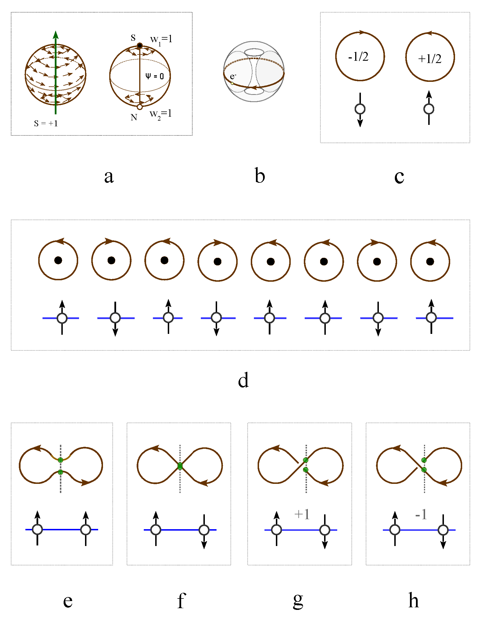
Figure 2.
(a) The closed loop on the surface of solid torus represents spinor wave function. The wavefunction and the conjugate wavefunction of (b) topological spin , (c) topological spin , (d) topological vacuum state and (e) topological vacuum state . (f) Three coupled topological spin states with .
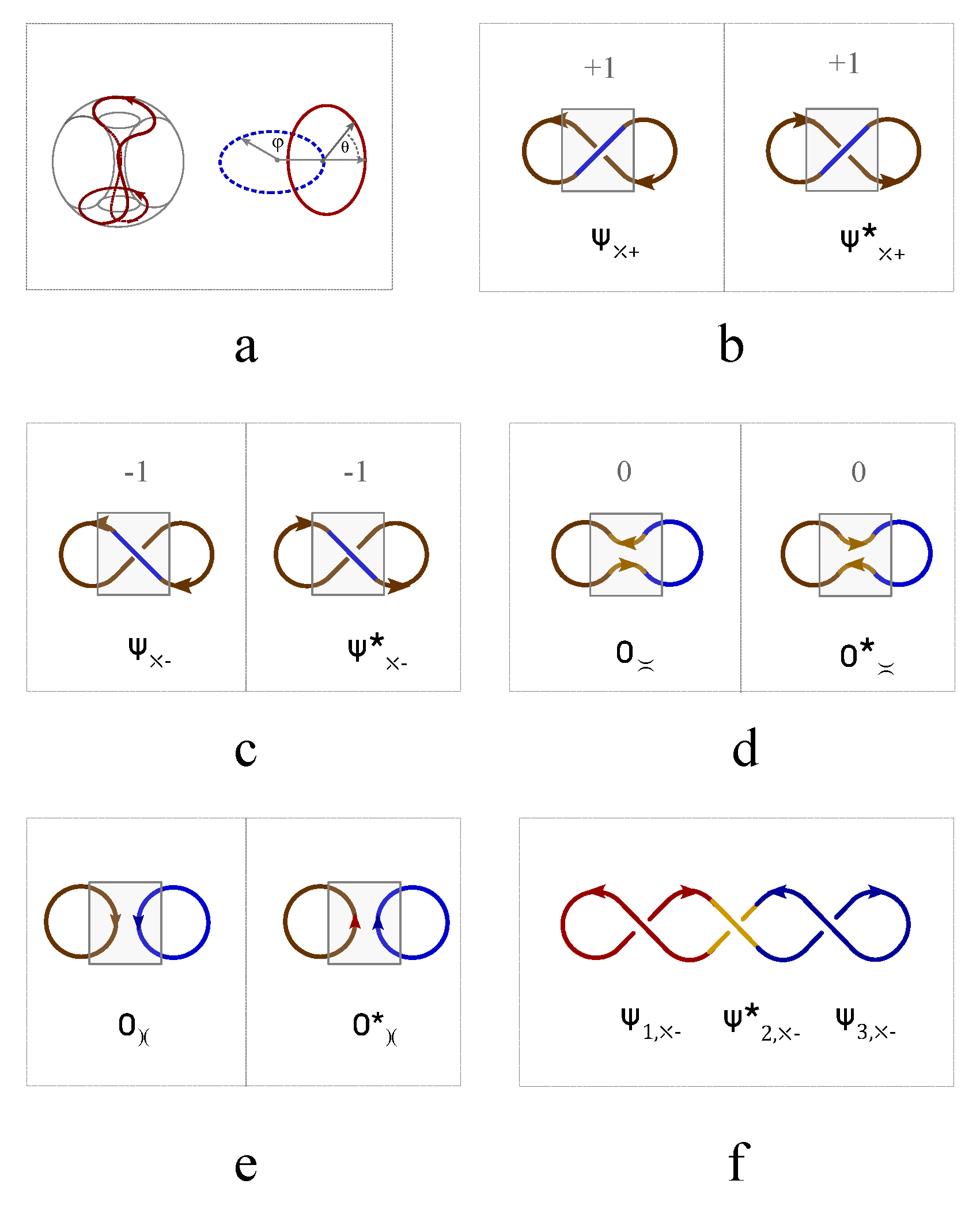
Figure 3.
(a) The knot configuration of two coupled spins. (a) , (b) , (c) , (d) , (e) , (f) .
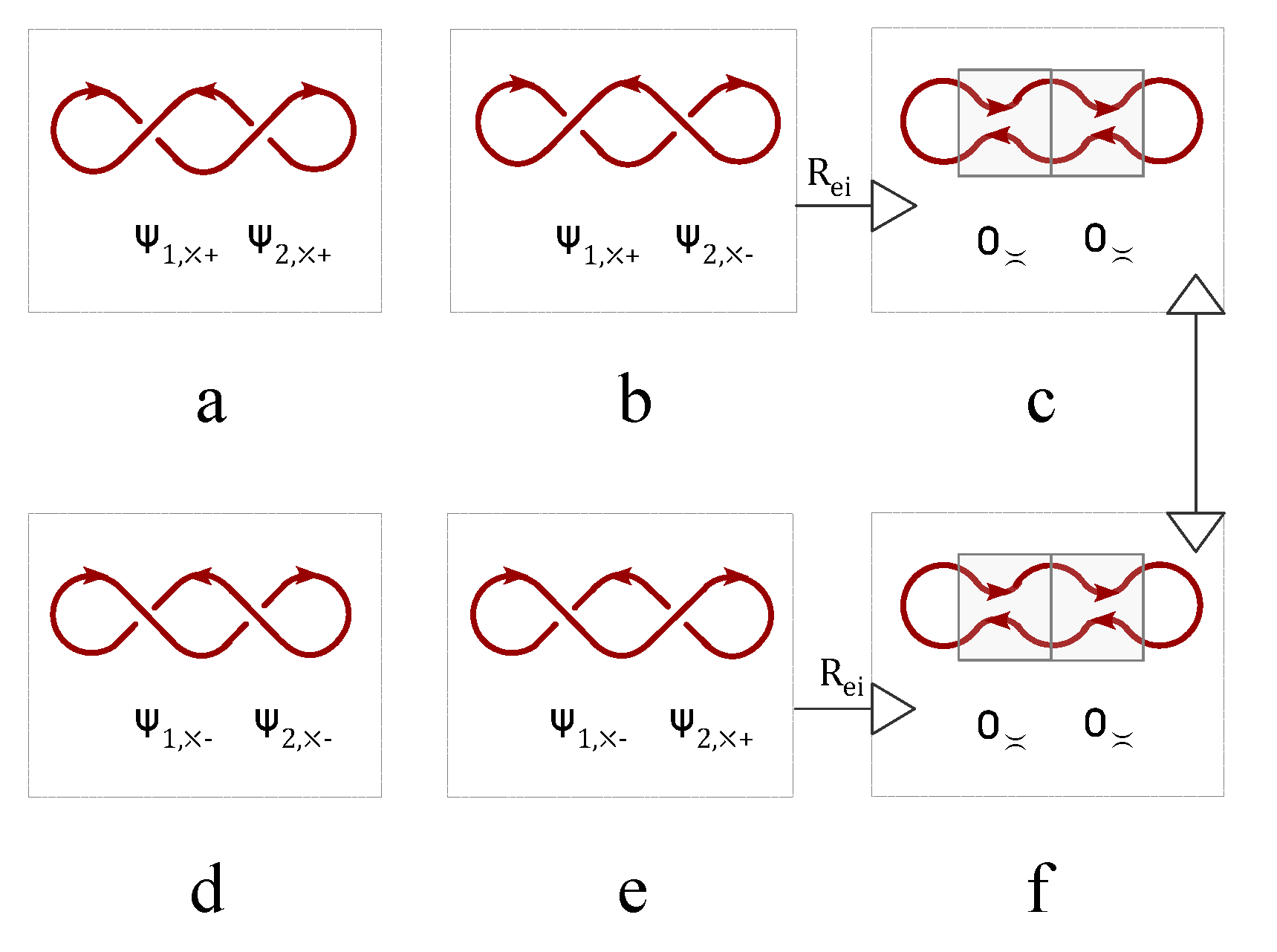
Figure 4.
(a) A crossing has four open endings. (b) The vacuum states with positive topological spin and its conjugation in (c). (d) The vacuum state with negative topological spin and its conjugate in (e). (f) The "8"-shaped knot. (g) The ∞-shaped knot. (h) The complex knot with 12 endings. (i) The intersecting current lines.
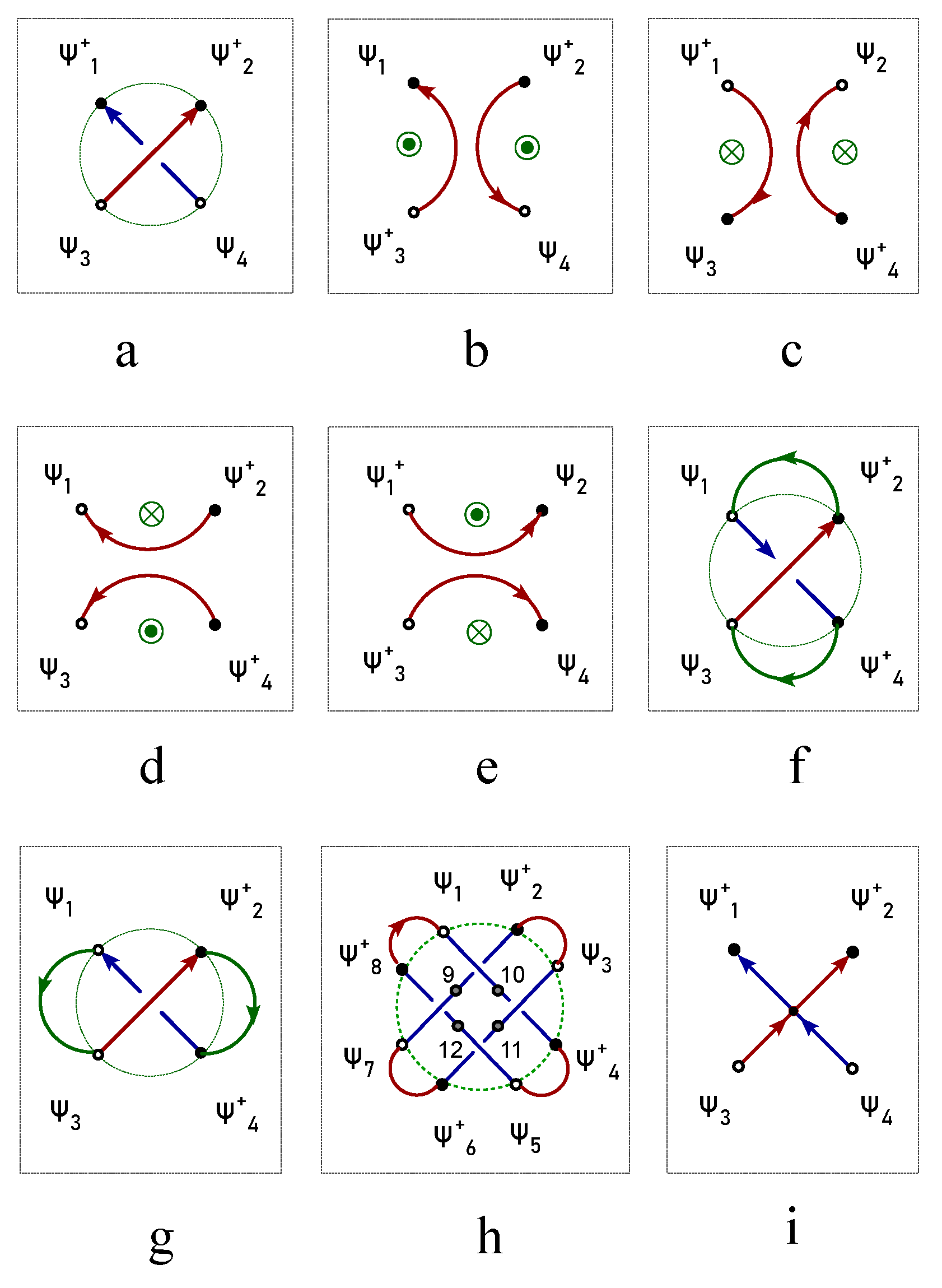
Figure 5.
The right handed trefoil knot state decomposes into eight possible full vacuum states .
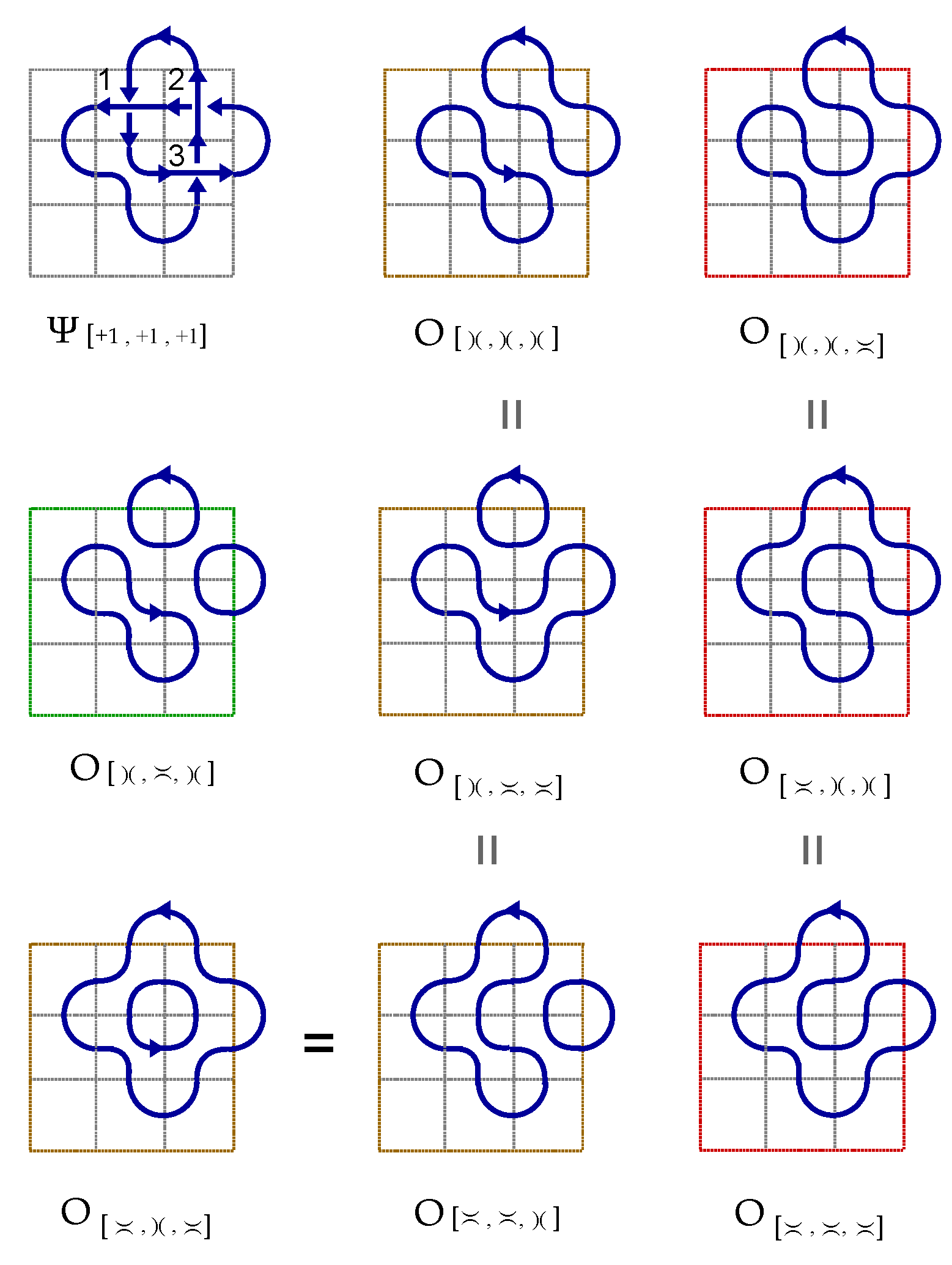
Figure 6.
The evolution of Jones polynomial with parameter t. The blue (red) curve indicates the right (left) handed trefoil knot.
Figure 6.
The evolution of Jones polynomial with parameter t. The blue (red) curve indicates the right (left) handed trefoil knot.
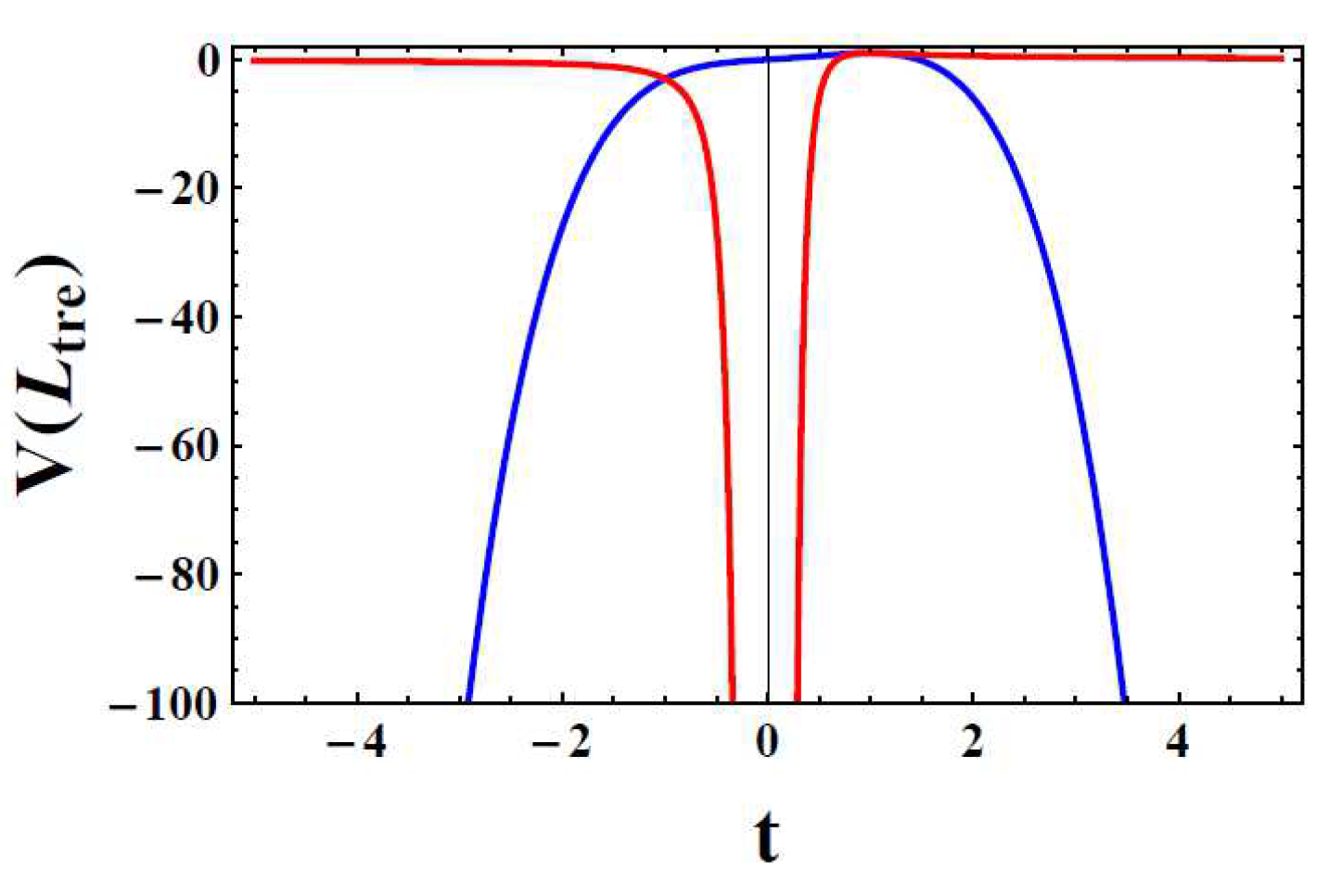
Figure 7.
(a) Connecting the ending points of the four fluxes reorganized them into a left handed trefoil knot. (b) The boundary flux lines penetrates through the laminar surface in cross section and . The knot in (a) is equivalently mapped into (c) a left-hand trefoil and (d) its topological equivalent knot in three dimensional space.
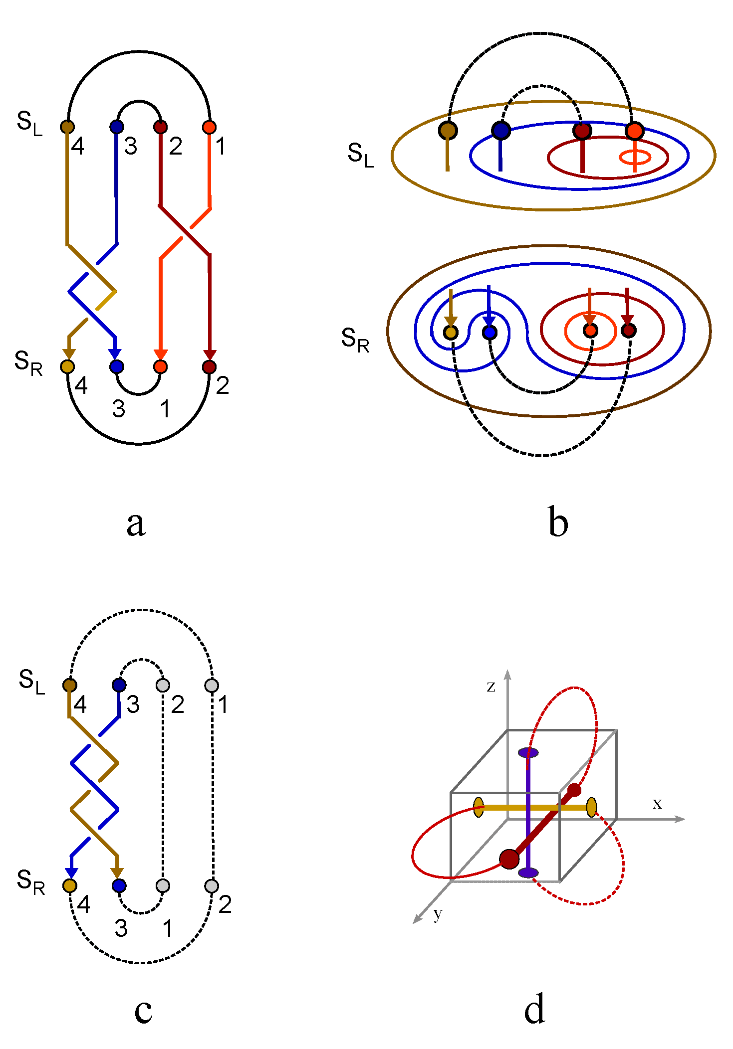
Figure 8.
Exemplar knots with three crossings, which are labeled by wavefunction of three topological spins ().
Figure 8.
Exemplar knots with three crossings, which are labeled by wavefunction of three topological spins ().
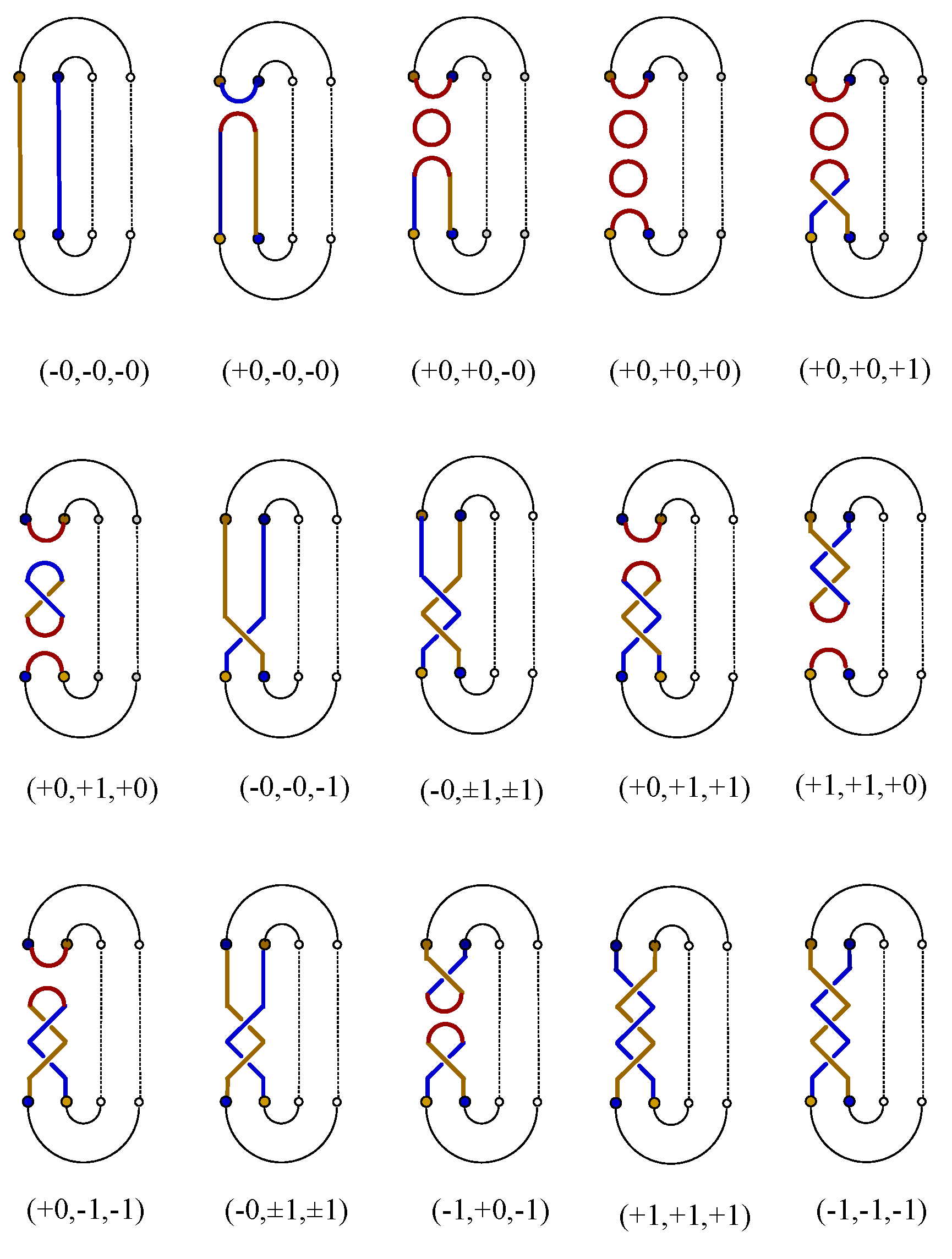
Figure 9.
The thermodynamic entropy of the left-hand trefoil knot with the eigenenergy of knot defined by.
Figure 9.
The thermodynamic entropy of the left-hand trefoil knot with the eigenenergy of knot defined by.
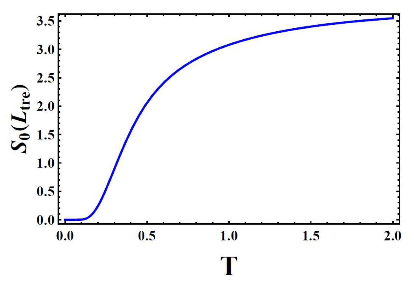
Figure 10.
The von Neumman entropy of the right-hand trefoil knot (indicated by the blue curve) drops to zero at zero temperature. The entropy of the left-hand trefoil knot (the red curve) drops to zero at finite temperature.
Figure 10.
The von Neumman entropy of the right-hand trefoil knot (indicated by the blue curve) drops to zero at zero temperature. The entropy of the left-hand trefoil knot (the red curve) drops to zero at finite temperature.
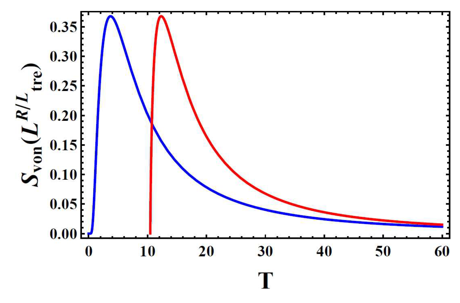
Figure 11.
(a) The induced magnetic field loop by knotted electric current loops. (b) Eliminating one crossing of electric loop generates one crossing of magnetic loop. (c) Generating one more crossing of electric loop creates one more crossing of magnetic loop. (d) The one dimensional spin chain with antiferromagnetic coupling and (e) ferromagnetic coupling.
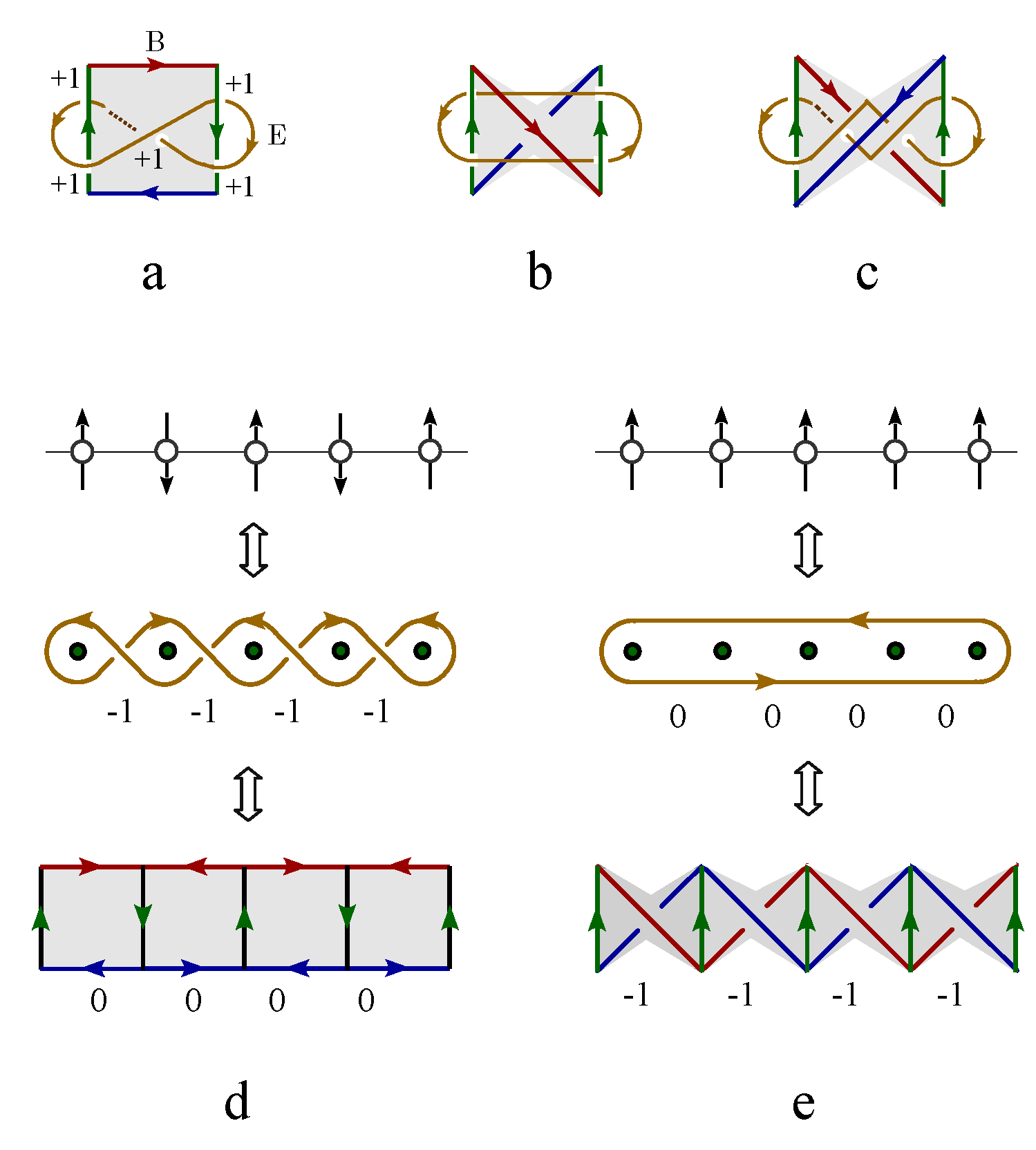
Figure 12.
(a) A spin liquid state is represented by Ising spin chain. (b-c-d) The spin liquid state is equivalently represented by a magnetic knot lattice. (e) The magnetic knot lattice is equivalently represented by two winding magnetic fluxes that are wrapped by electric laminar layers. The cross section of the winding laminar layers is an exactly Thurston’s train track pattern.
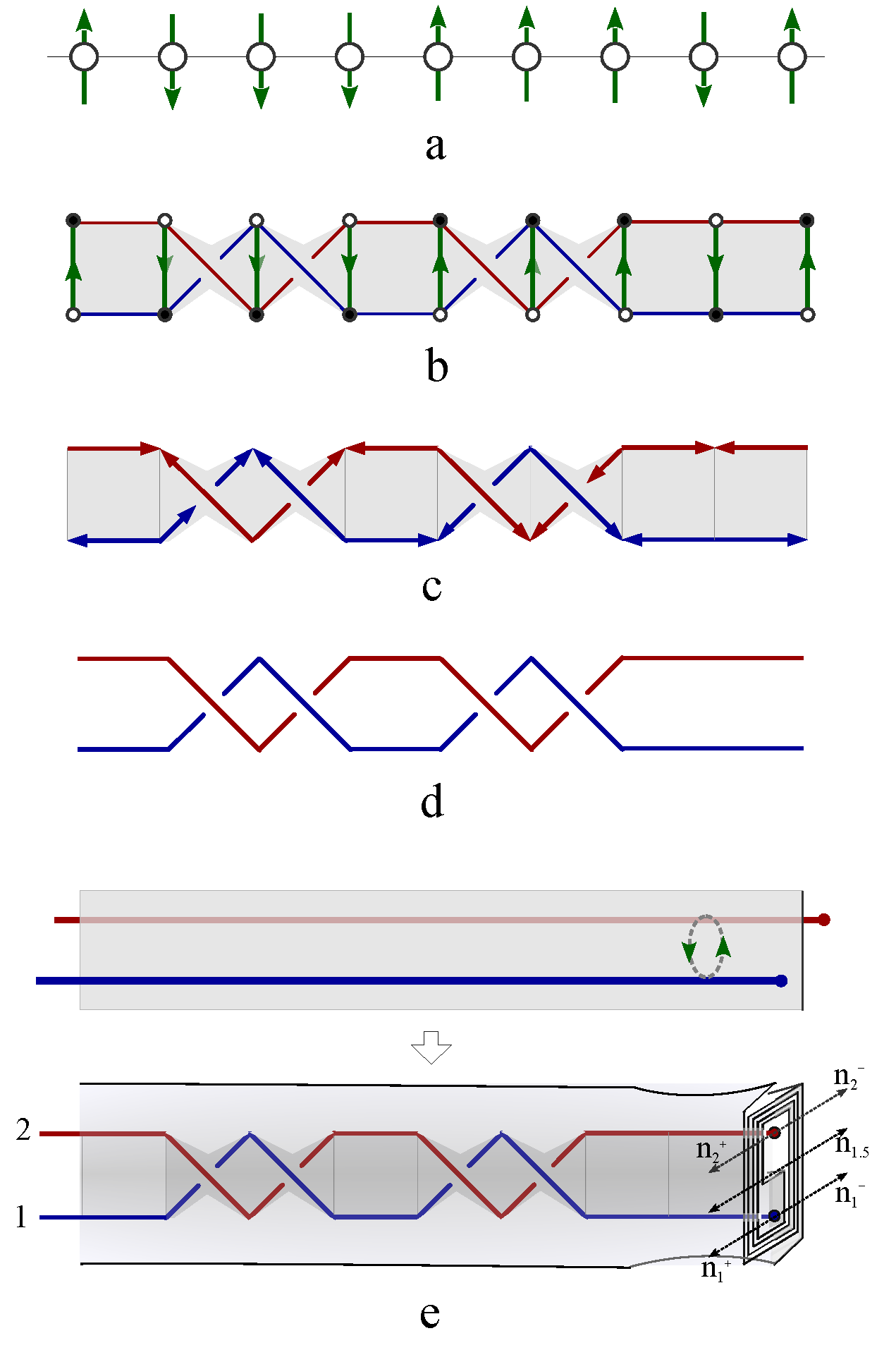
Figure 13.
(a) The spin liquid state with one kink separating two ferromagnetic domains. (b) The annihilation of the kink fuses the two ferromagnetic domains into one domain. (c) The annihilation of two topological kinks generated two opposite crossings.
Figure 13.
(a) The spin liquid state with one kink separating two ferromagnetic domains. (b) The annihilation of the kink fuses the two ferromagnetic domains into one domain. (c) The annihilation of two topological kinks generated two opposite crossings.
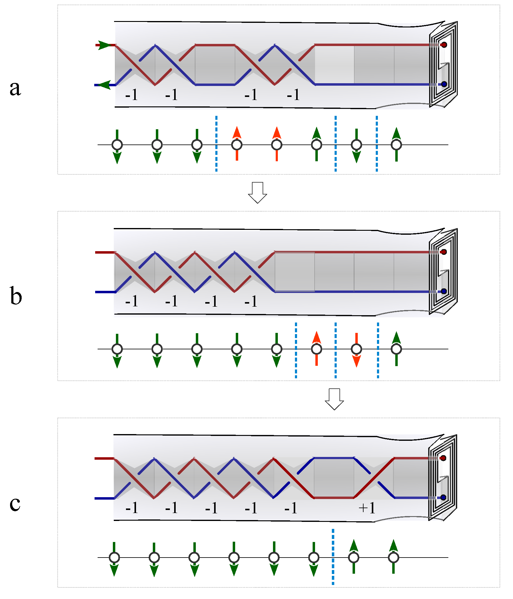
Figure 14.
(a) The two magnetic fluxes are separated by an electric laminar layer. (b) The two magnetic flux rings units into one ring with one self-crossing. (c) The two magnetic current configurations with respect to the two eigenvalues of spin. (d) The spin 0 state with a vortex pair generated by local fluctuation. (e) The spin 1 state with two self-crossings. (f) The total spin 0 state is the sum of a state and a state. (g) The total spin - state is the sum of a spin 1 state and one spin .
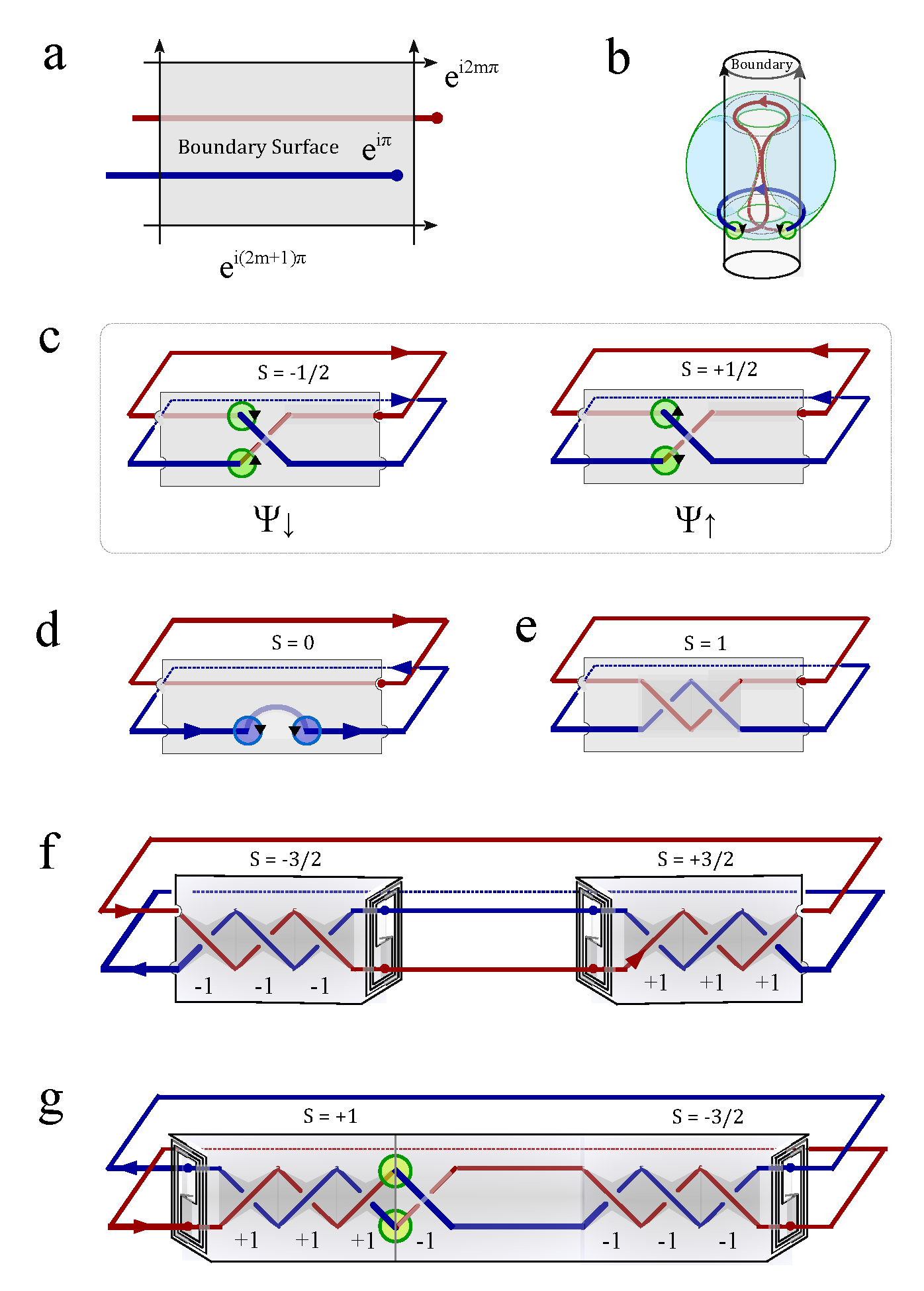
Figure 15.
(a) The overcrossing, under crossing and crossing avoiding states. (b) The one dimensional lattice of alternating knots. The bulk spin chain is consists of (c) even and (d) odd number of spins. (e) A twisted hyperbolic surface is generated by opposite braiding on the two endings. (f) Unfolding the twisted hyperbolic lamination into a flat monolayer transfers the knot lattice to the other half surface of the torus.
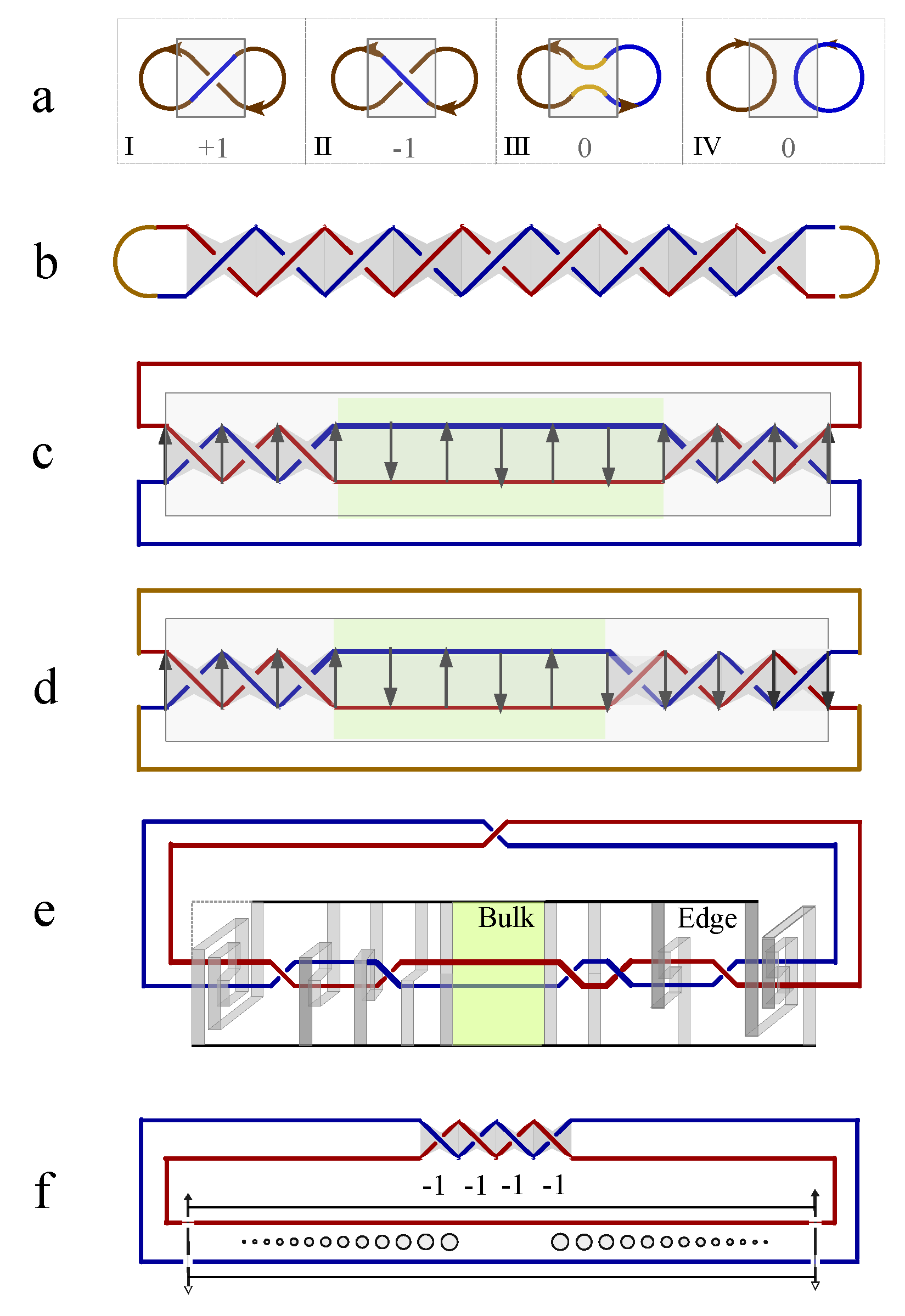
Figure 16.
(a) The double hyperbolic pseudosphere surface of electron fluid is generated by fixing its middle point and braiding its endings on the left (right) hand side in clockwise (counterclockwise) direction. (b) The double hyperbolic pseudosphere surface generated by braiding two closed flux loops and its deformation during unfolding operations.
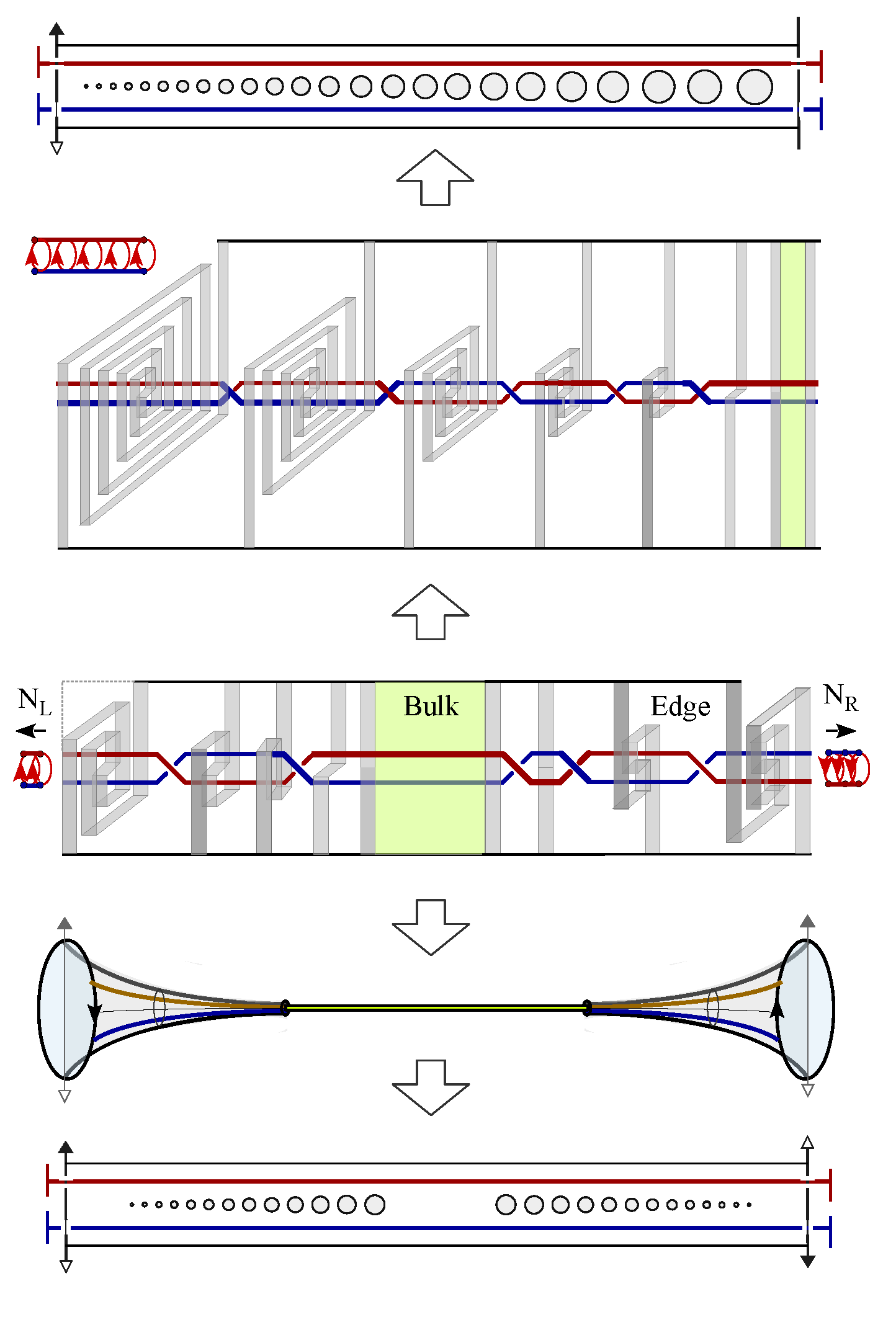
Figure 17.
(a) A hyperbolic surface of electron fluid is generated by braiding the left endings of flux pair with its right endings fixed. (b) The double hyperbolic surface of electron fluid is generated by braiding the middle point of flux pair with its both endings on the left and right hand side fixed. (c) The inverse double hyperbolic surface of electron fluid is generated by fixing its middle point and braiding its endings on both the left and right hand side in the same direction.
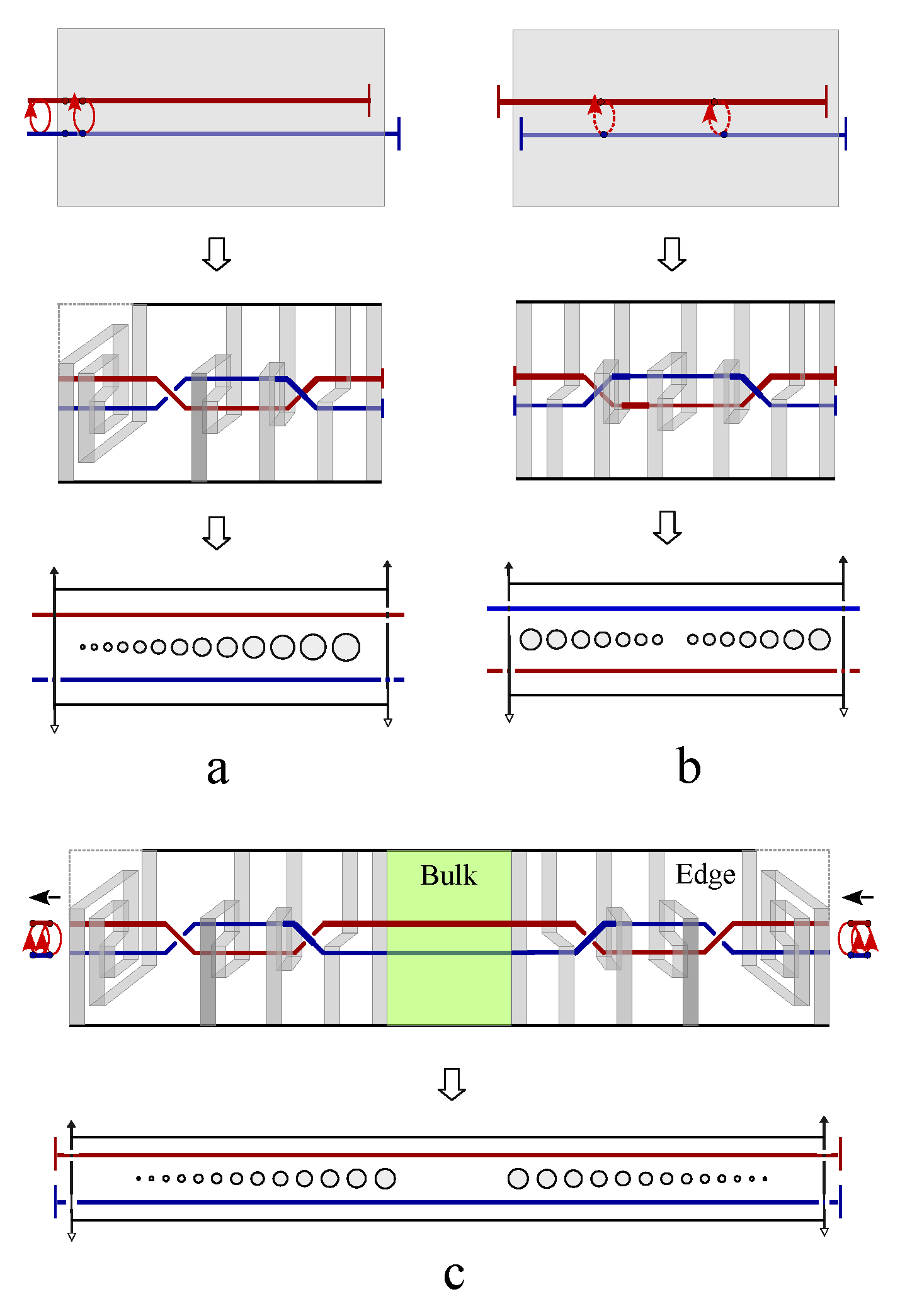
Figure 18.
The resultant resistivity with respect to the edge lamination in Figure 17c decreases to zero as the braiding number m grows to infinity. The unit of the resistivity is .
Figure 18.
The resultant resistivity with respect to the edge lamination in Figure 17c decreases to zero as the braiding number m grows to infinity. The unit of the resistivity is .
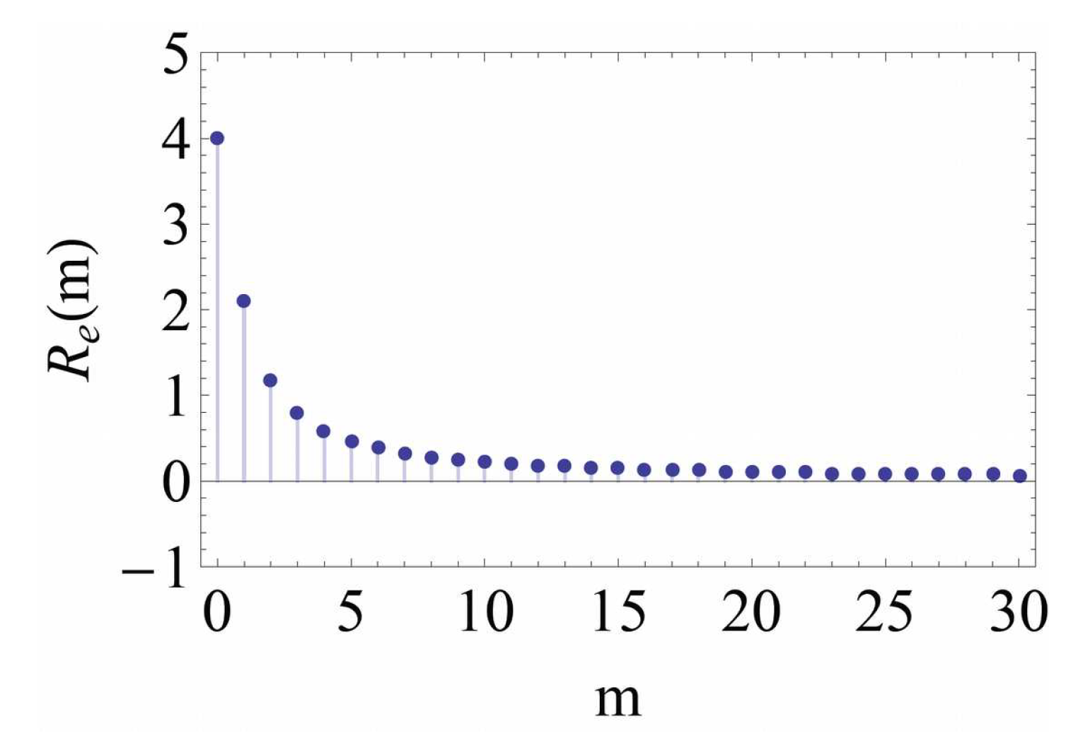
Figure 19.
The resultant resistivity on the left edge increases to the maximal value as electrons approach to the left boundary with respect to the lamination in Figure 16a.
Figure 19.
The resultant resistivity on the left edge increases to the maximal value as electrons approach to the left boundary with respect to the lamination in Figure 16a.
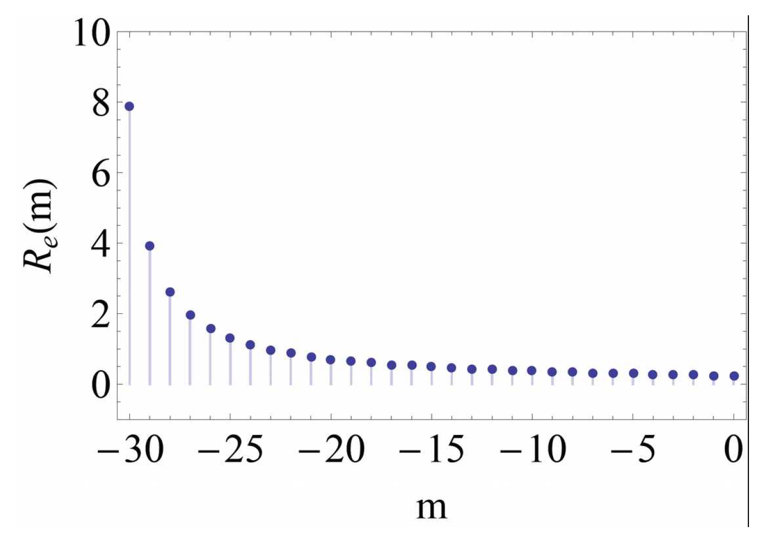
Figure 20.
(a) An antiferromagnetically coupled spin chain. (b) A local braiding on the magnetic segment generates a pair of fermionic kink excitations with opposite topological charge. (c) The two kinks moves in opposite direction with the same energy unit. (d) a pair of anyon is generated out of vacuum state. (e) The anyon pair is separated by a local braiding operation and run into opposite direction.
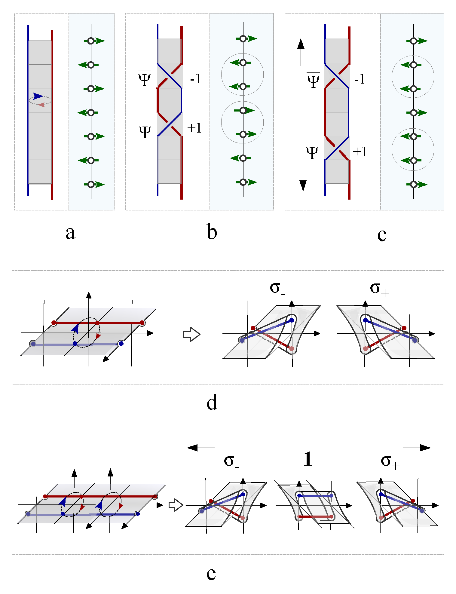
Figure 21.
(a) A vacuum particle fuses with one anyon into another anyon. (b) Two anyons with opposite charge fuses into a vacuum particle. (c) Two identical anyons fuse into a fermionic quasiparticle.
Figure 21.
(a) A vacuum particle fuses with one anyon into another anyon. (b) Two anyons with opposite charge fuses into a vacuum particle. (c) Two identical anyons fuse into a fermionic quasiparticle.
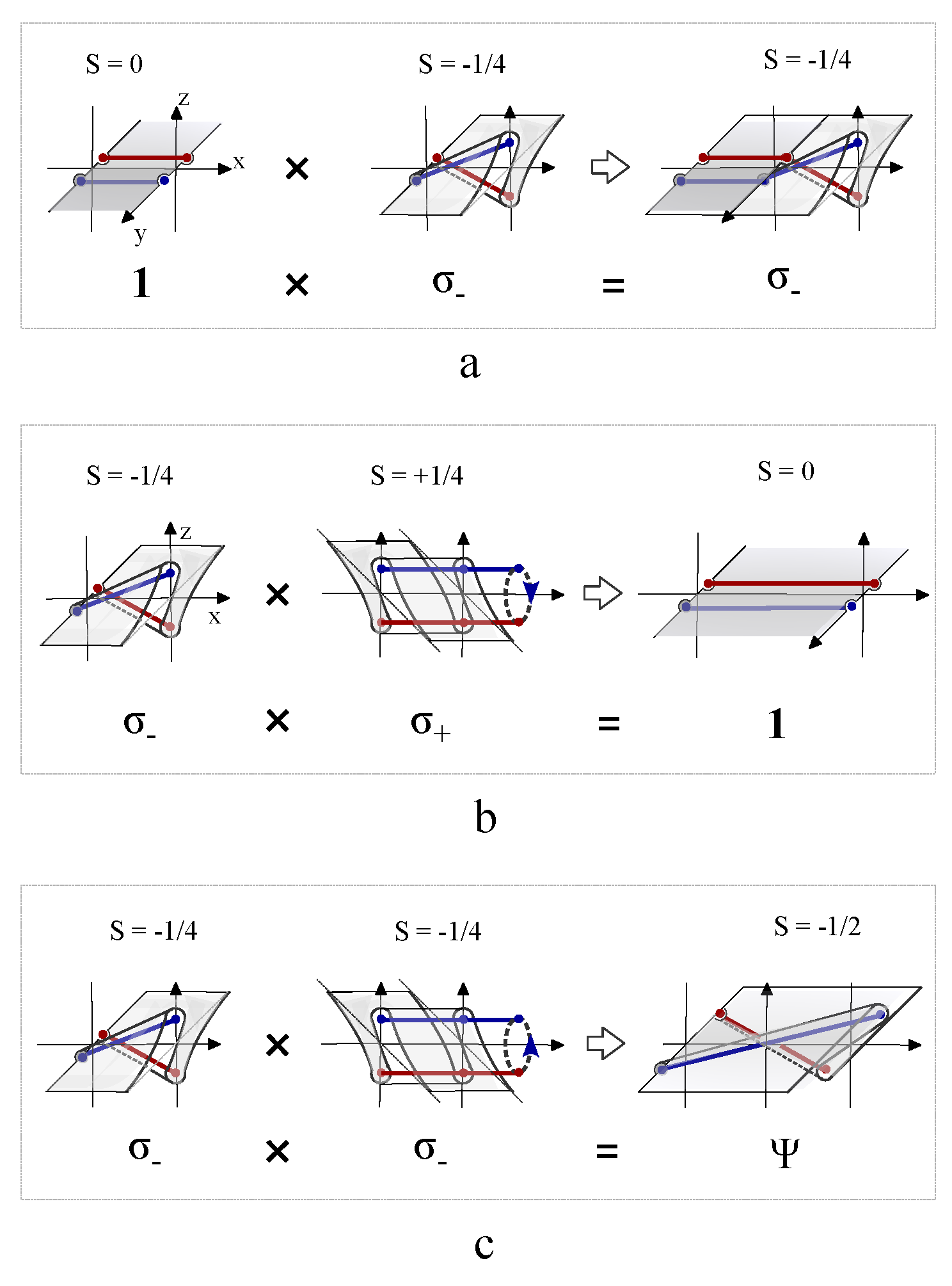
Figure 22.
(a) The one dimensional spin chain form a standing electric current wave sandwiched in between two magnetic fluxes, and is equivalently mapped into one dimensional chain of many current bonds. (b) The current chain folds into train tracks with five layers of stacked parallel current bonds. (c) Seven layers of antiparallel currents with a pair of fluxes located at the innermost gaps. (d) The flux hops to the second innermost gaps in opposite direction. (e) The flux hops to the outermost gaps. (f) The phase distribution along the one dimensional chain sandwiched in between two fluxes.

Figure 23.
The total electromagnetic interaction energy of one dimensional spin chain of many antiparallel current bonds.
Figure 23.
The total electromagnetic interaction energy of one dimensional spin chain of many antiparallel current bonds.
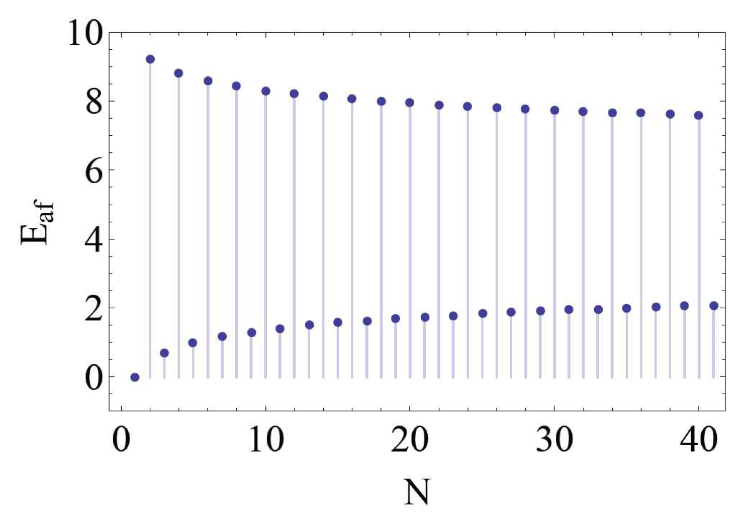
Figure 24.
(a) The one dimensional spin chain is folded as a spiral train track of state. (b) When two fluxes hop outward to the outermost gap zone, it forms an effective vortex pattern of with a freely fluctuating spin chain in between the two fluxes. (c) Both the two fluxes hop to the open free zone to represent an integral filling state. (d) The shortest path from A to B. (e) Two exemplar paths covering all lattice sites. (f) The one dimensional spin chain transform into two dimensional Ising model by introducing the coupling bonds between chain segments.
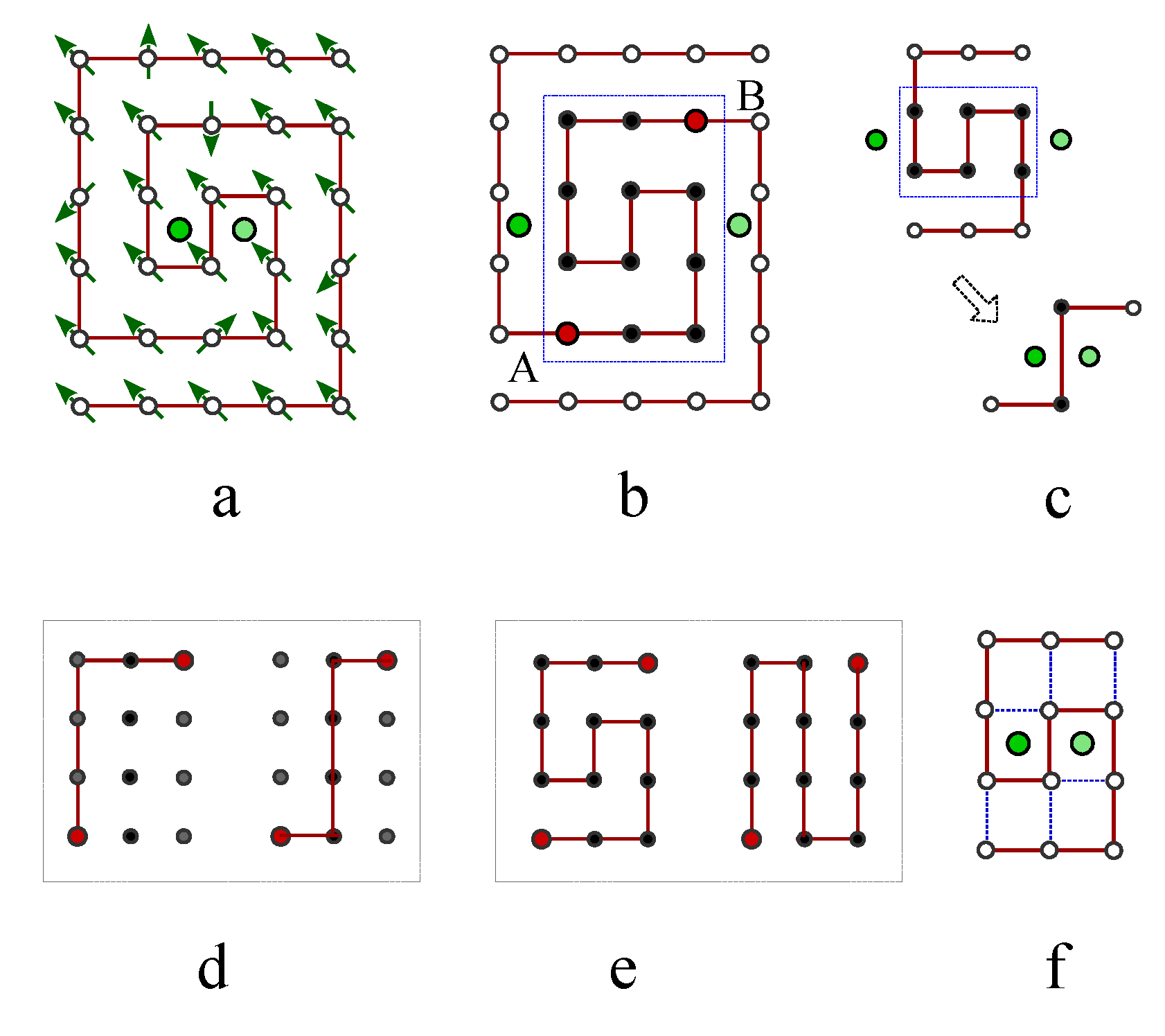
Figure 25.
(a) Two vortices of the same vorticity fuse into one big vortex. (b) Two vortices of opposite vorticity fuse into an open spiral vortex pattern under dislocation of flux pair. (c) A square lattice of vortices is generated by translation unit vortex with double core. (d) Global dislocation of the vortex lattice in (c) generates a square lattice of spiral vortices connected to one another.
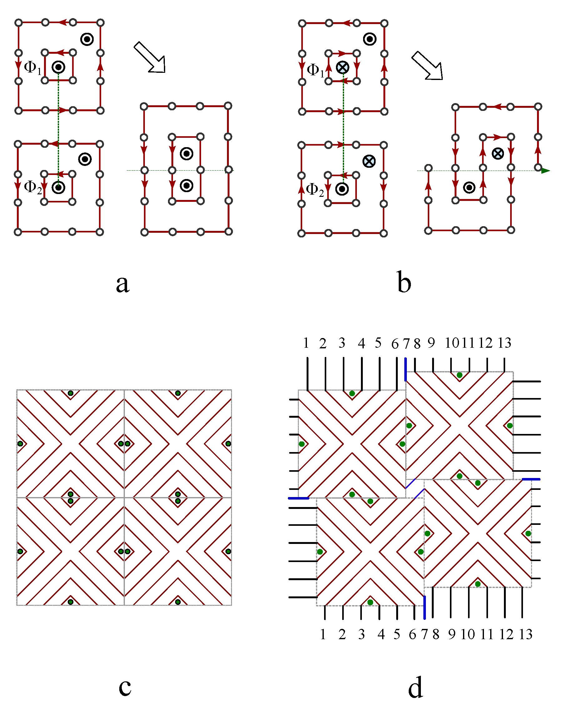
Figure 26.
The effective critical temperature with respect to different filling factors, diverges at half-filling state .
Figure 26.
The effective critical temperature with respect to different filling factors, diverges at half-filling state .
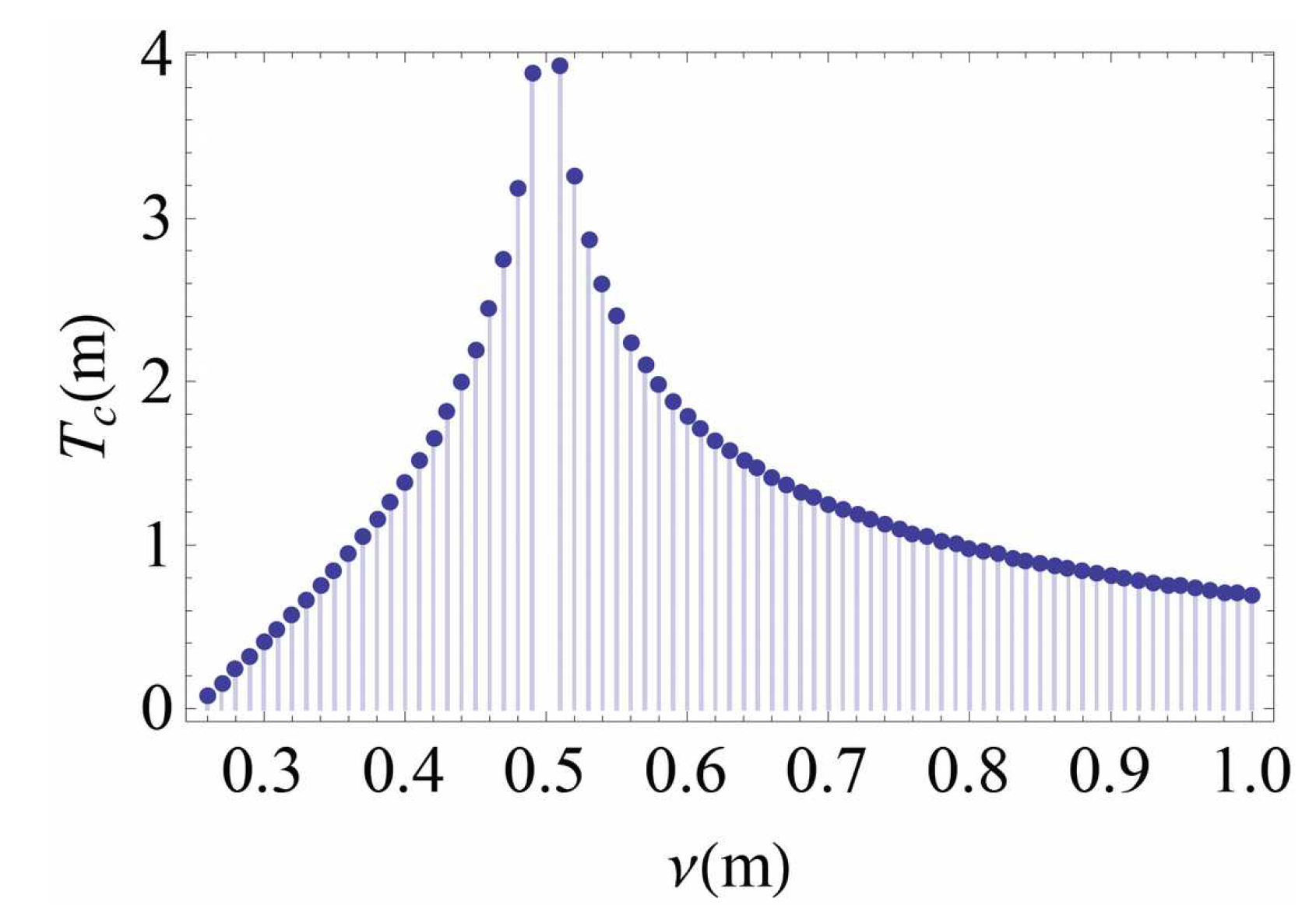
Figure 27.
(a) Braiding the two antiparallel magnetic fluxes counterclockwisely generates folded electric laminations with fractional charge . (b) Braiding the two antiparallel magnetic fluxes counterclockwisely twice generates folded laminations with fractional charge . (c) Braiding the two antiparallel magnetic fluxes clockwisely twice generates fractional charge .
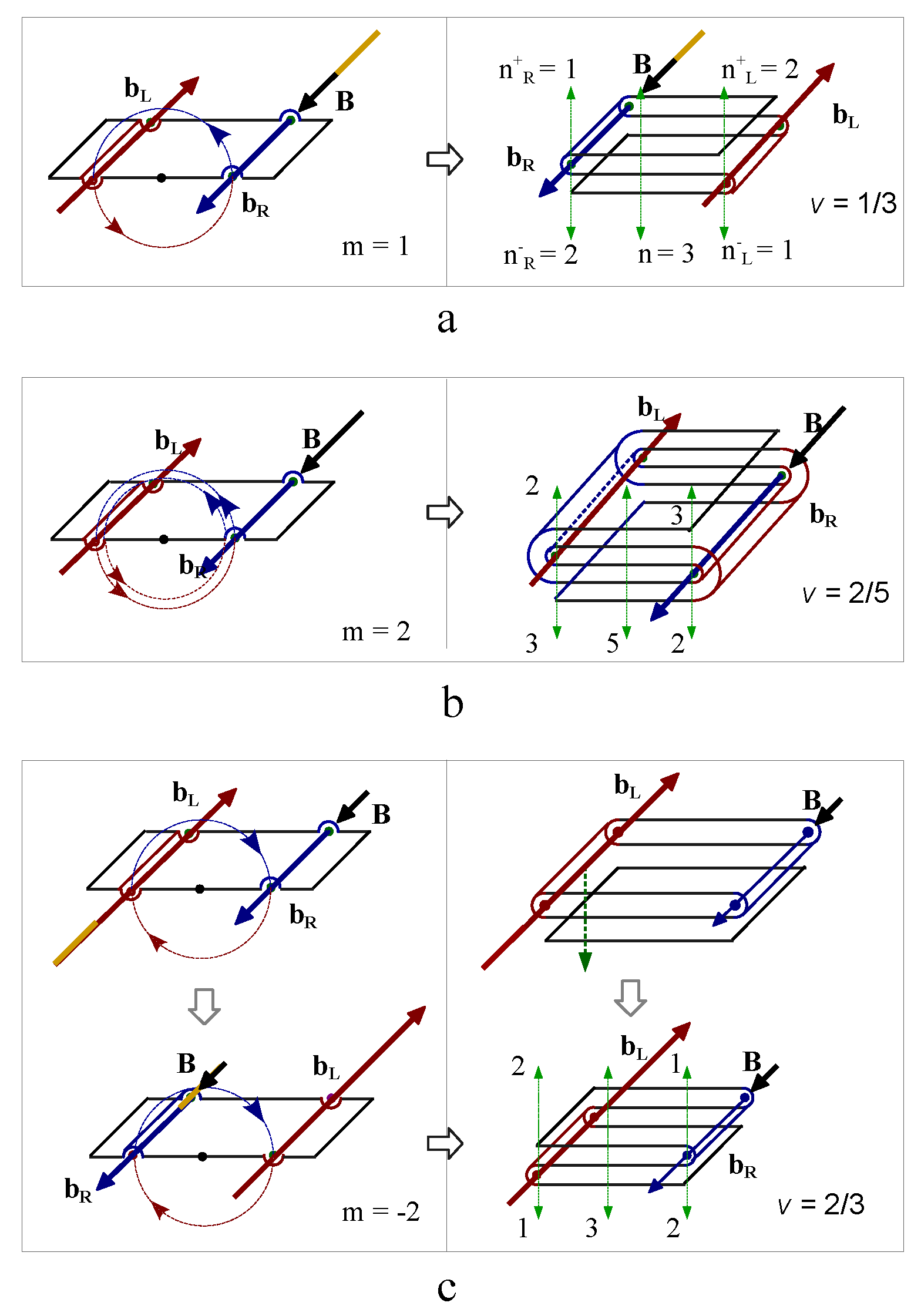
Figure 28.
(a) The first electric loop flows around the magnetic flux pair and is cut into two half tracks along the middle line between the flux pair. (b) The left half track and the right half track are reconnected to form a train track. (c) Each of the three train track segments carries a gauge potential vector . (d-e-f) one counterclockwise braiding generates the train track of fractional charge . (g) Two electric loops flow around the magnetic flux pair. The first (second) loop carries gauge potential and generates gauge field vector . (h) Cutting the two electric loops and reconnecting them constructs the train track of . (i-j) The train track of can be generated by two continuous counterclockwise braiding.
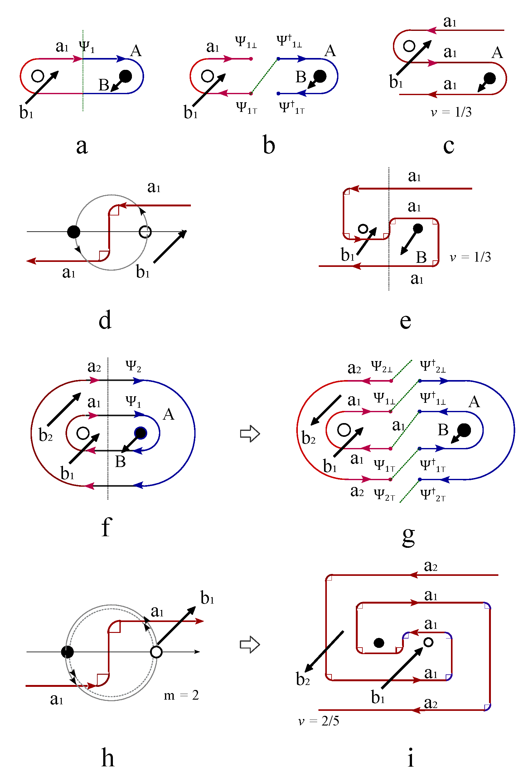
Figure 29.
(a) The collective train track pattern of state is generated by dislocation of magnetic flux lattice. (b) The train track of state is generated by squeezing two pairs of fluxes into one unit space under braiding operations. (c) The train track of state is directly generated by squeezing four nearest neighboring fluxes into one column. (d) The train track of is generated by squeezing six nearest neighboring fluxes into one column. (e) Braiding three pairs of fluxes into one condensed flux bundle generates the train tracks of .
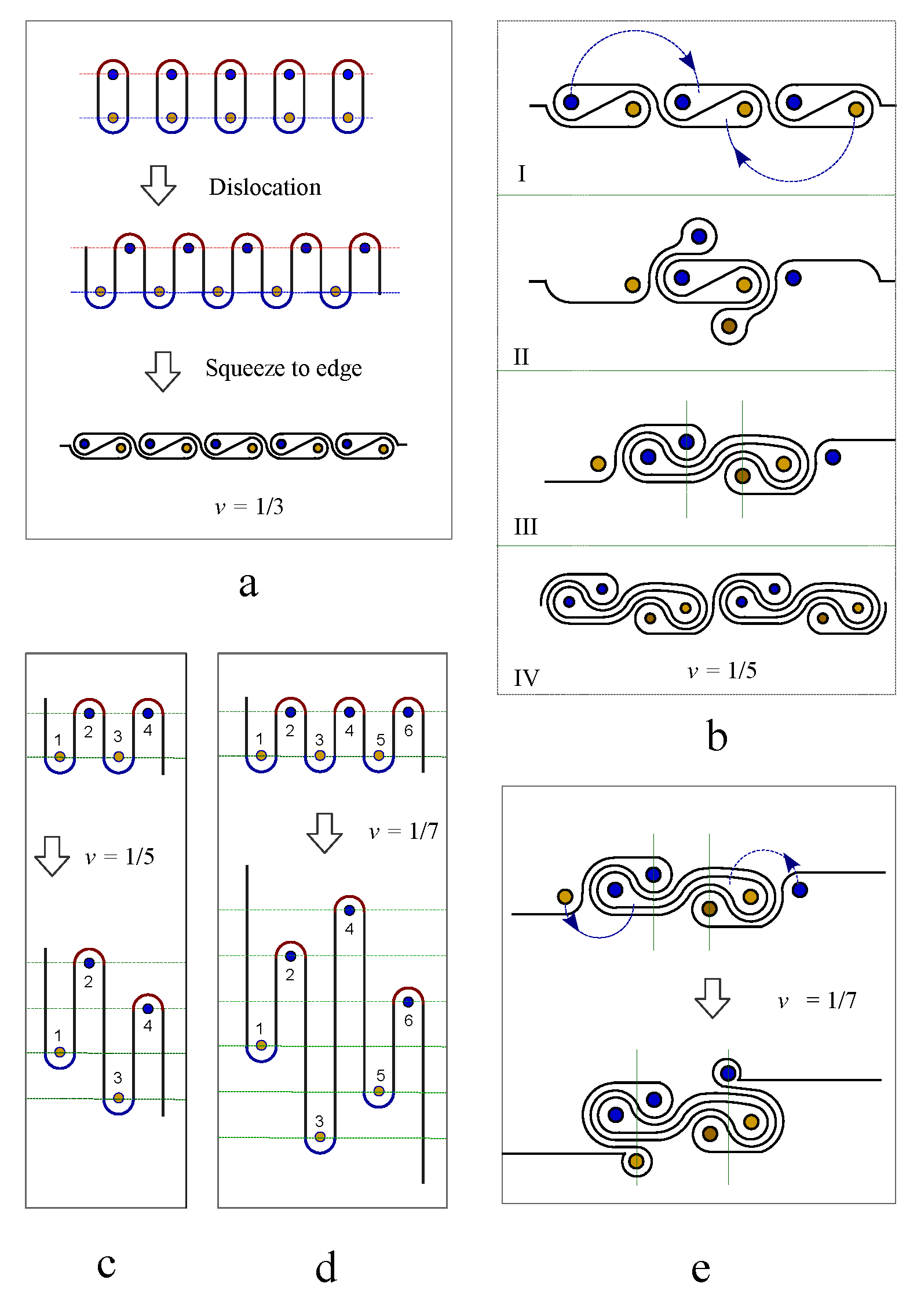
Figure 30.
(a) The global train track pattern of state and (b) the global train track of state of a two dimensional electron fluid in high magnetic field. (c) The effective potential surface on the two dimensional electron gas.
Figure 30.
(a) The global train track pattern of state and (b) the global train track of state of a two dimensional electron fluid in high magnetic field. (c) The effective potential surface on the two dimensional electron gas.
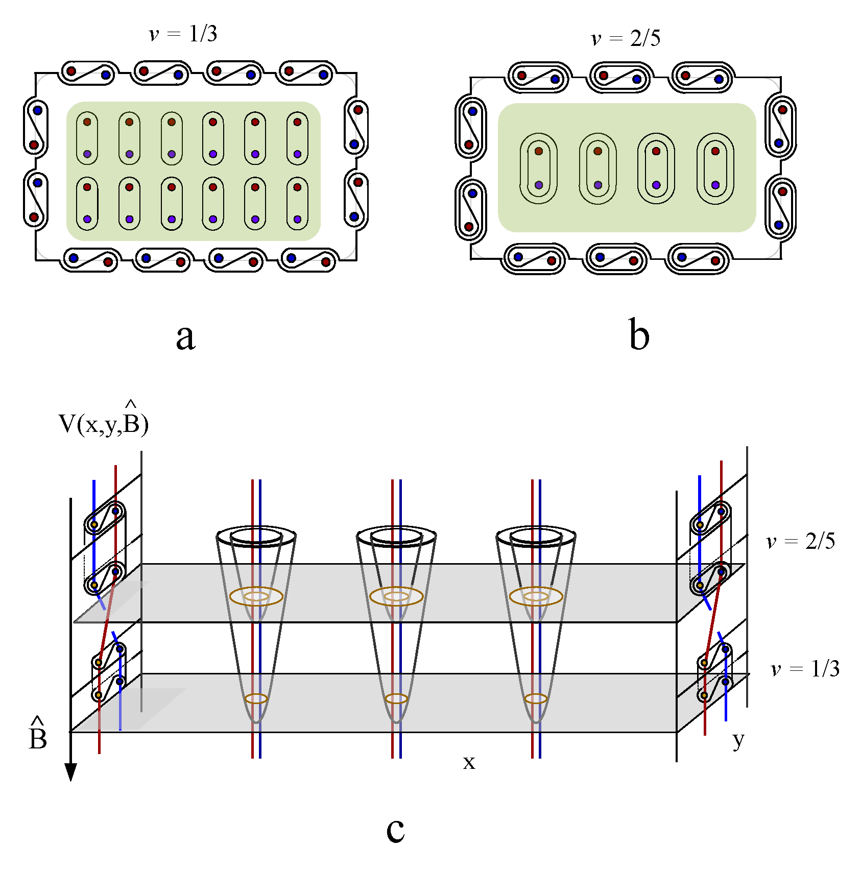
Figure 31.
(a) The fitting curve of absolute value of magnetic field strength against the quantum number m. (b) The fitting curve of oriented magnetic field against m. (c) The expanding electric laminar layer during the braiding process of magnetic flux pair. (d) The expanding electric laminar layer can be mapped into a electric hyperbolic surface. (e) The distance between two points of electric lamination grows exponentially with a decreasing magnetic field strength.
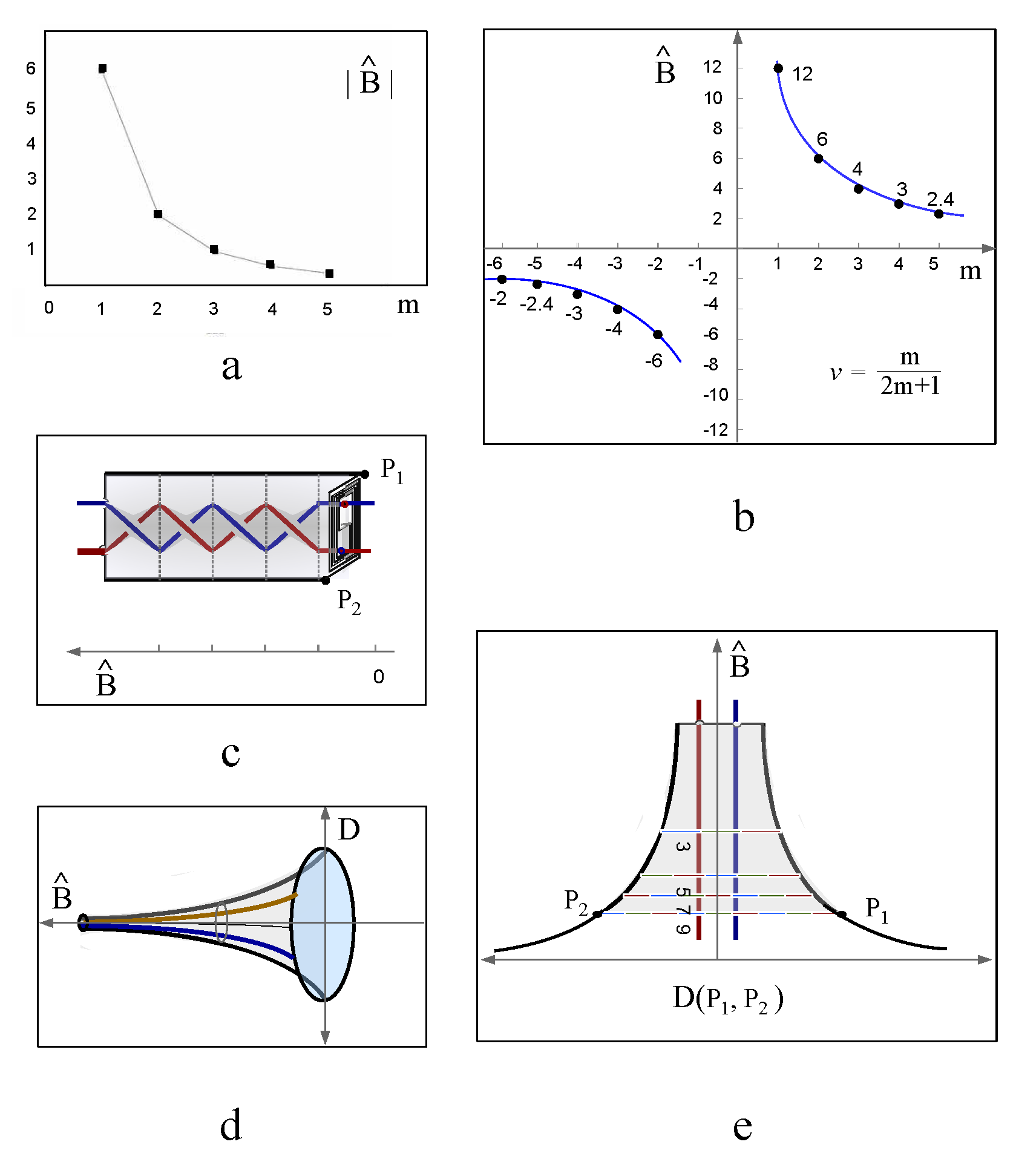
Figure 32.
(a) The growing train tracks and Hall conductance around the flux pair with respect to decreasing resultant magnetic field strength and Hall resistivity. (b) The electron laminar surface is projected into the double hyperbolic surface in the space of position against the effective magnetic field strength . (c) The approximated double hyperbolic space generated by one braiding and (d) two braiding on the middle flux segment. (e) Different contour cross sections of double hyperbolic surface are characterized by topological number m.
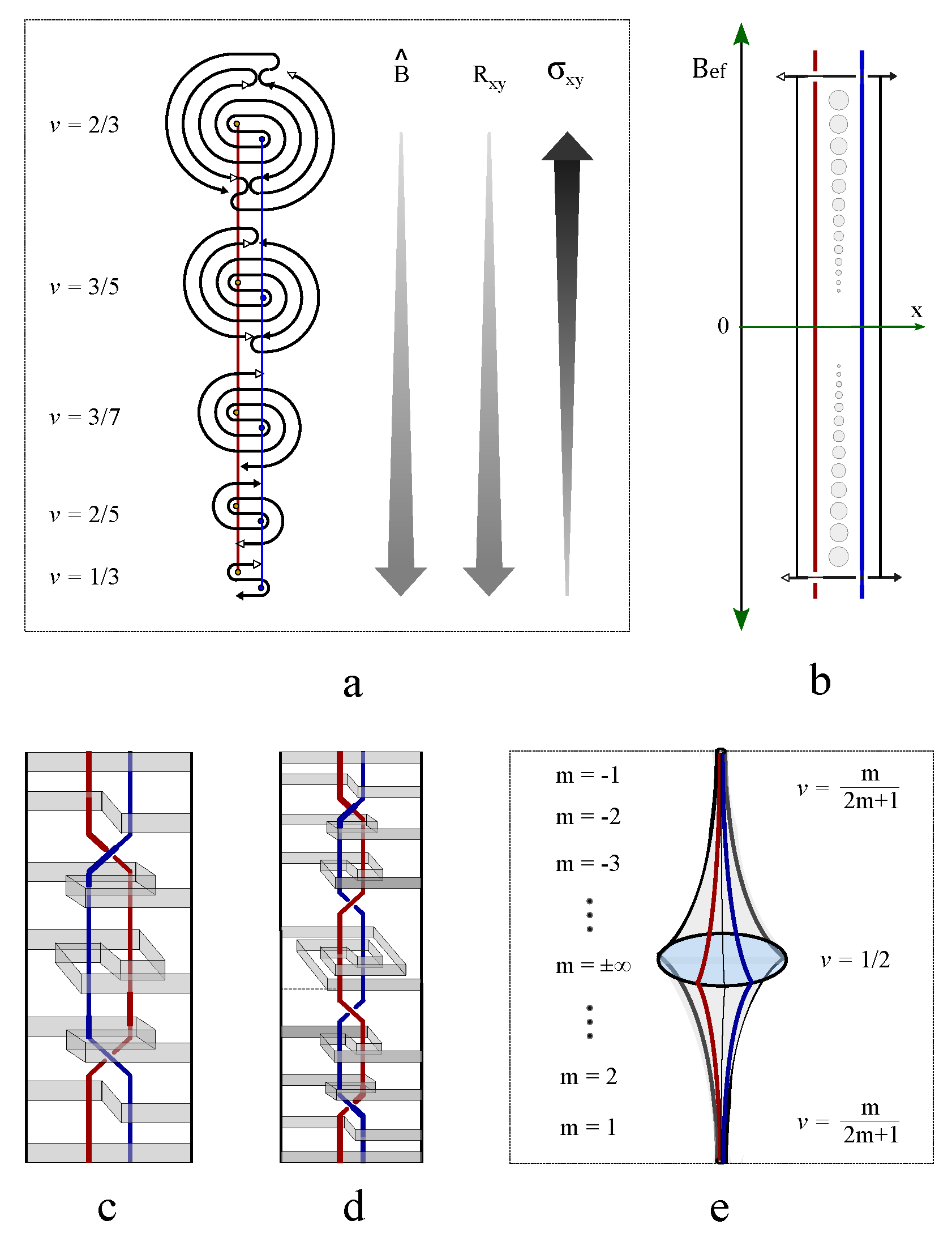
Figure 33.
The landscape of Landau levels in the bulk and the topological hyperbolic potential surface on the edge as a function of effective magnetic field .
Figure 33.
The landscape of Landau levels in the bulk and the topological hyperbolic potential surface on the edge as a function of effective magnetic field .
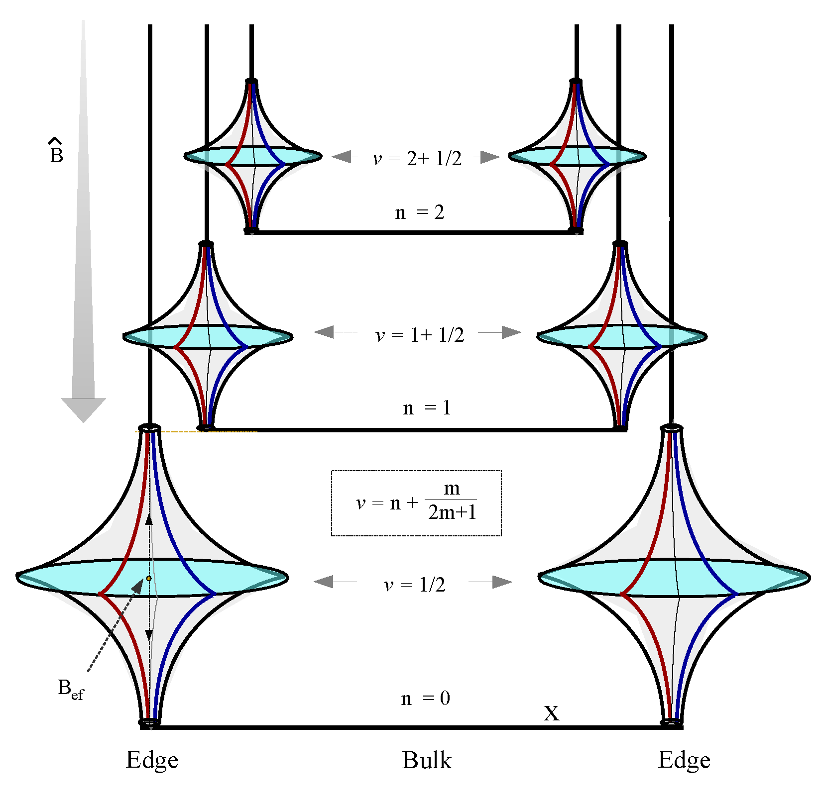
Figure 34.
(a) The fractional charge is generated by two steps of translation and reconnection of one track loop around magnetic flux pair. (b) The fractional charge is generated by two steps of translation and reconnection of three track loops. (c) The fractional charge generated by two steps of translations and reconnections of two track loops, and (d) by three steps of translations and reconnections of three track loops.
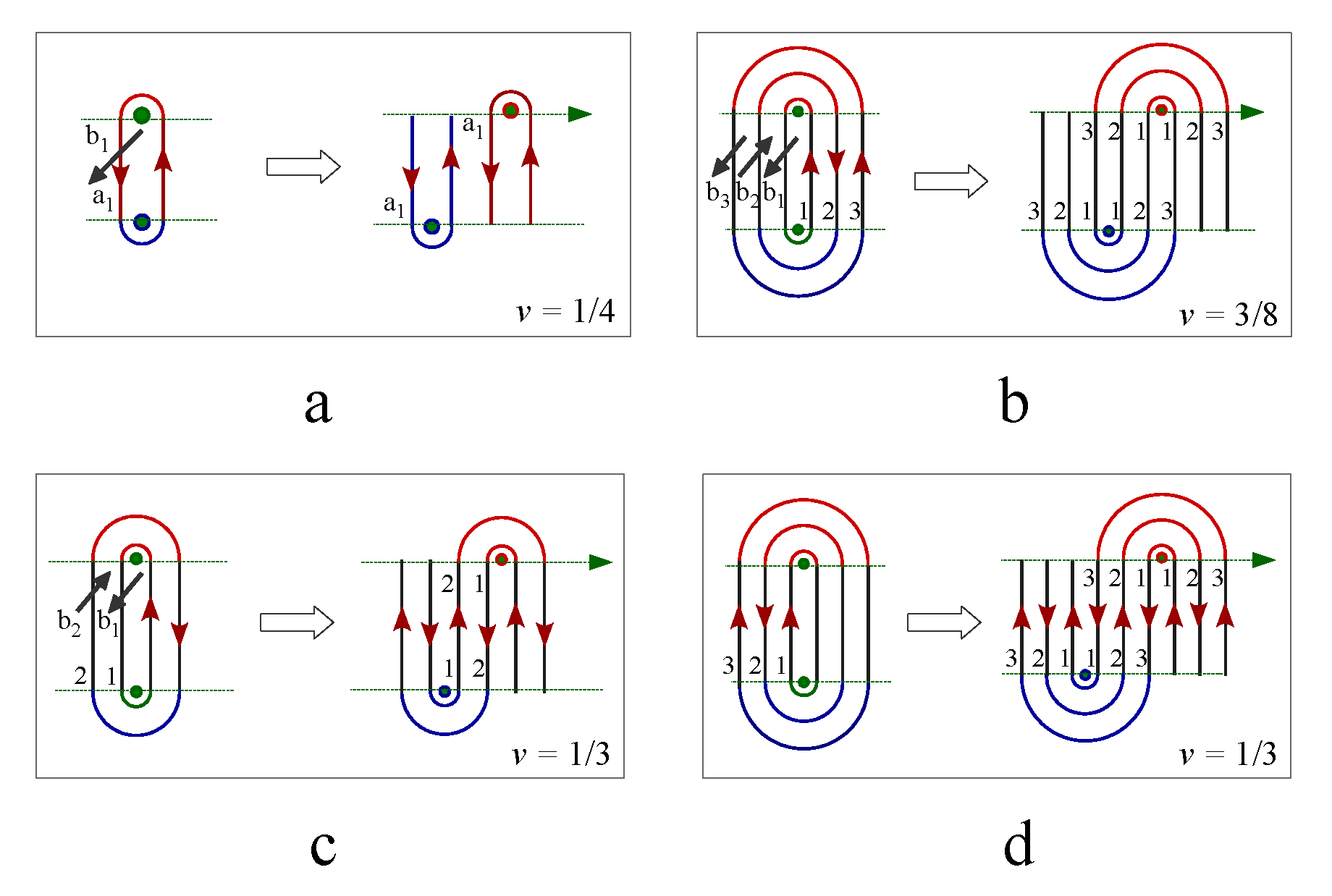
Figure 35.
(a) The bulk tracks collide with the open endings of edge tracks to contribute to the diagonal resistivity . (b) An inhomogeneous magnetic field strength is applied in z-direction to illustrate the hyperbolic surface of electron fluid laminations. (c) A conformal map of hyperbolic space to the plane of energy gap against spatial dimension x. The semicircle is geodesic curve.
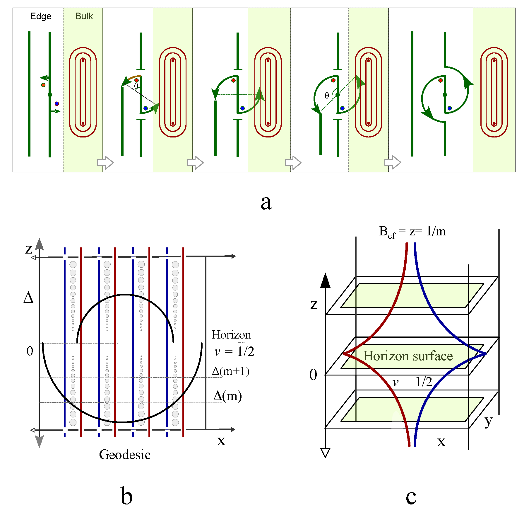
Figure 36.
The diagonal Hall resistivity oscillates with respect to real magnetic field strength in fractional quantum Hall effect according to Eq. (193).
Figure 36.
The diagonal Hall resistivity oscillates with respect to real magnetic field strength in fractional quantum Hall effect according to Eq. (193).
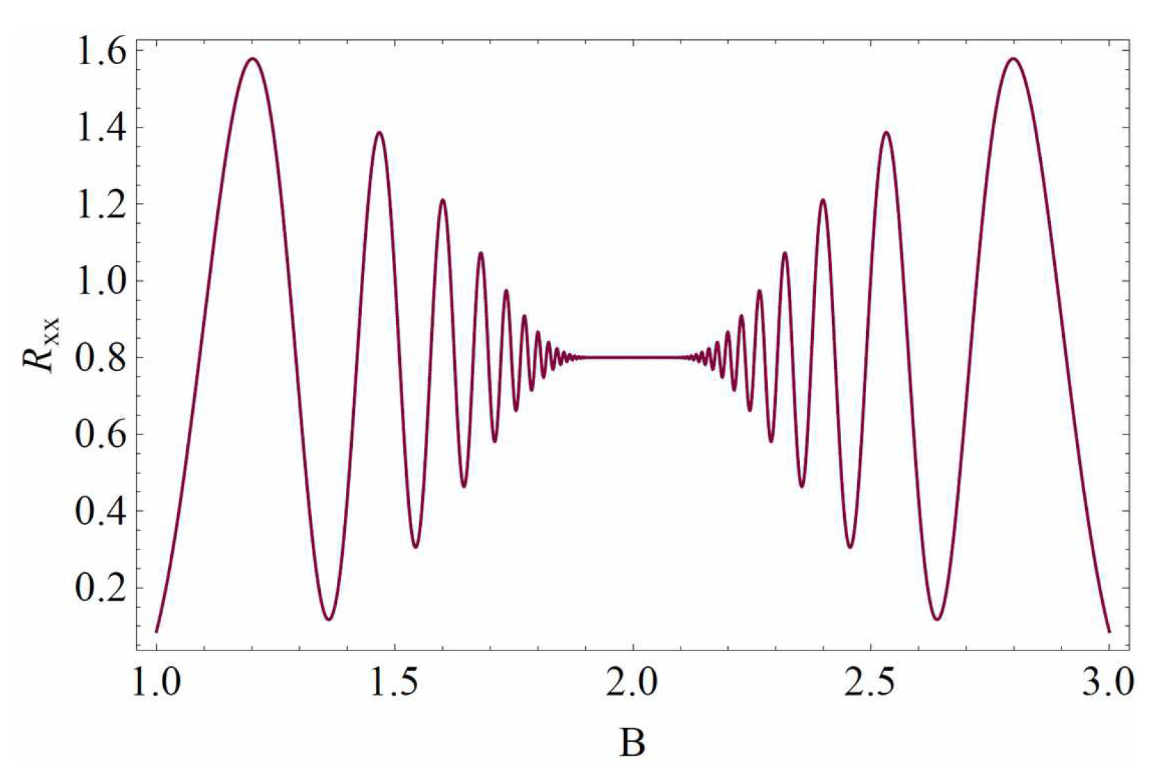
Figure 37.
The distance between two geodesic curves decays exponentially with respect to growing temperature.
Figure 37.
The distance between two geodesic curves decays exponentially with respect to growing temperature.

Figure 38.
(a) The electron sweeps over phase in top and bottom plane respectively. (b) The electron sweeps over fractional phase and in top and bottom plane respectively.
Figure 38.
(a) The electron sweeps over phase in top and bottom plane respectively. (b) The electron sweeps over fractional phase and in top and bottom plane respectively.
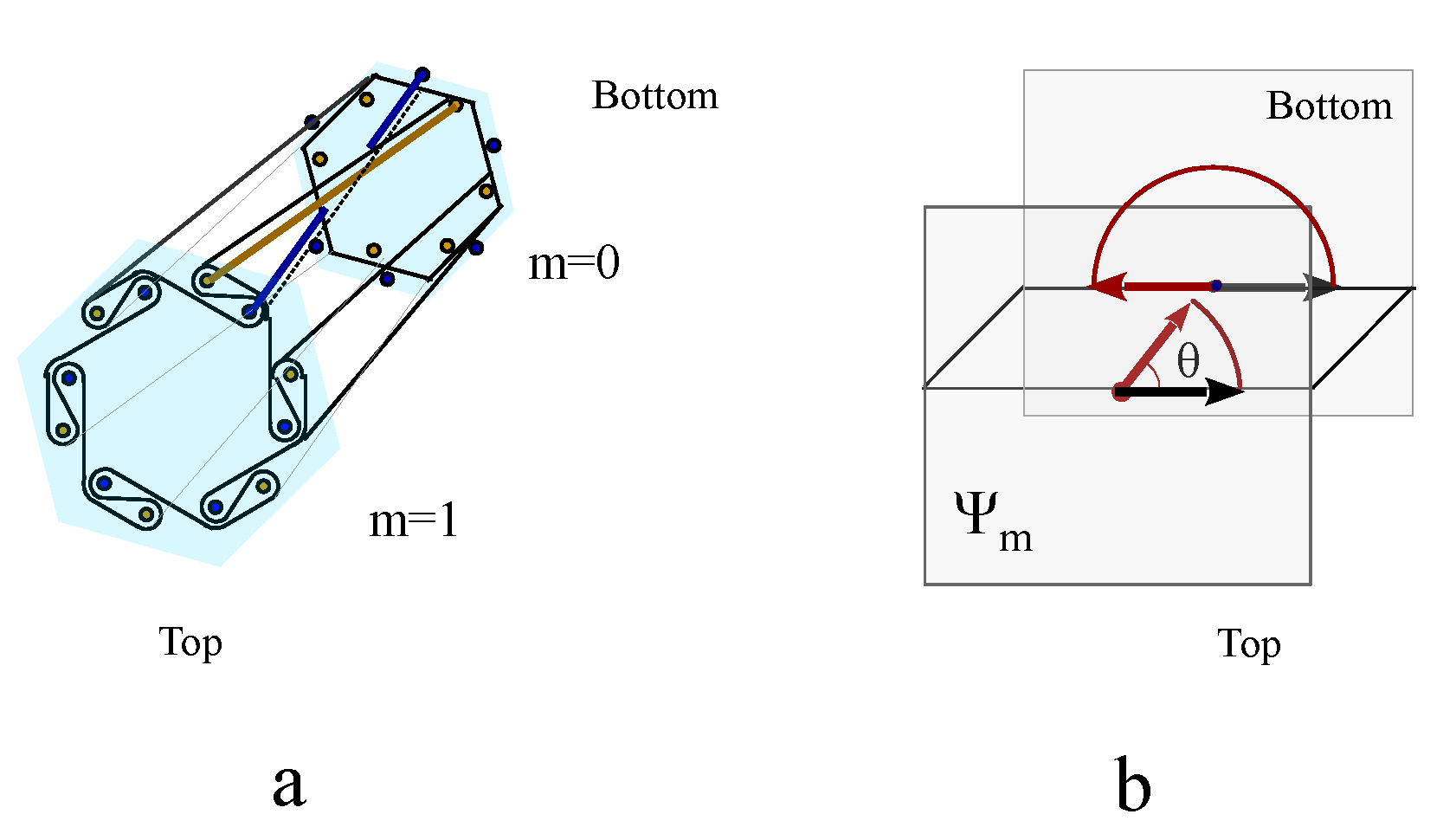
Figure 39.
(a) The sweeping angle of the Fermi arc in bottom plane. (b) The dual sweeping angle in the top plane.
Figure 39.
(a) The sweeping angle of the Fermi arc in bottom plane. (b) The dual sweeping angle in the top plane.
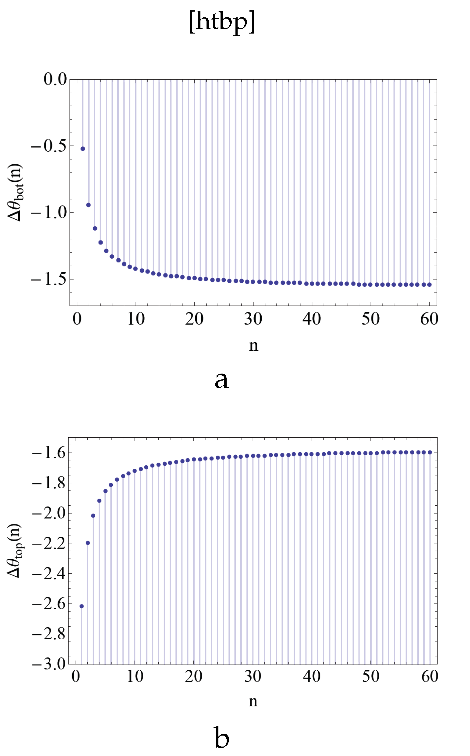
Figure 40.
(a) The hall resistivity tensor in three dimensional magnetic field is plotted according to Eq. (233) for .
Figure 40.
(a) The hall resistivity tensor in three dimensional magnetic field is plotted according to Eq. (233) for .
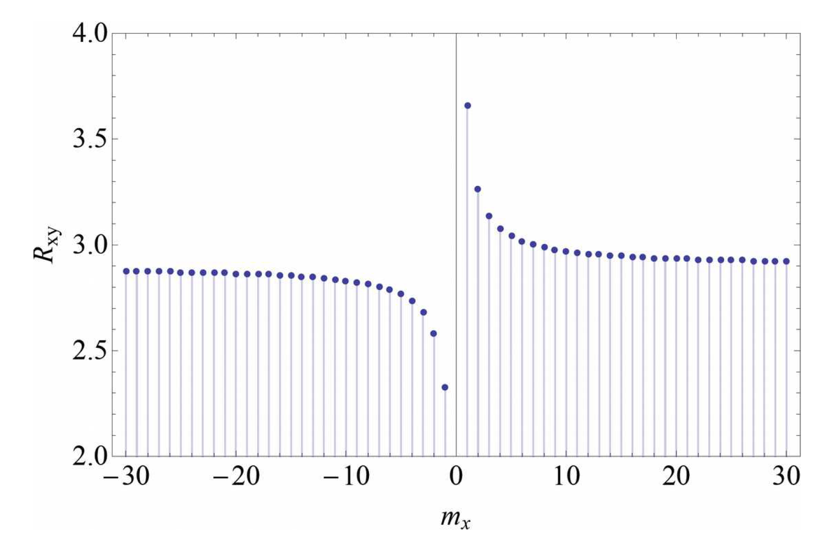
Figure 41.
The fractional filling factor against at a fixed value of .
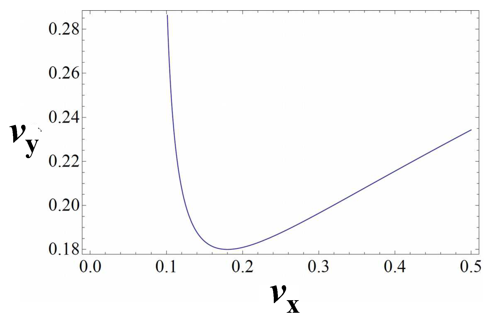
Figure 42.
(a) A laminar layer of electron fluid is sandwiched in between two pairs of magnetic fluxes, that are oriented in x- and y-axis respectively. (b) Braiding the two fluxes in y-axis folds the single layer into stacked three layers. (c) Braiding the two fluxes in x-axis over the stacked three layer folds the laminar layer into a lamination with nine layers. (d) The top view of laminar electron fluid after two braiding operations.
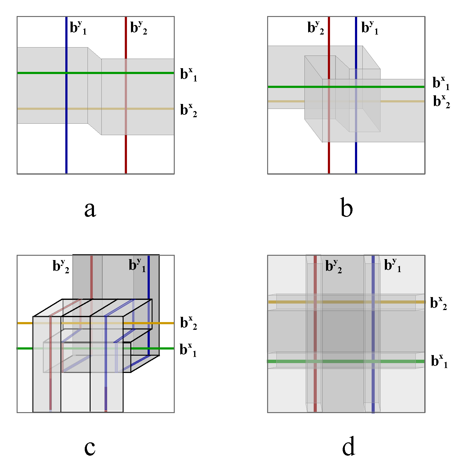
Figure 43.
(a) Two intersecting laminations map into two vacuum states in which two laminations avoid crossing. (b) The two magnetic fluxes (oriented in y-axis) on the opposite sides of lamination is wrapped by a tubular surface that intersects the lamination. Mapping the two intersecting states to two identical vacuum state generates folded lamination of three layers. (c) The folded lamination of five layers are generated by mapping two layers of tubular surface. (d) The folded lamination generated by further braiding fluxes along x-axis.
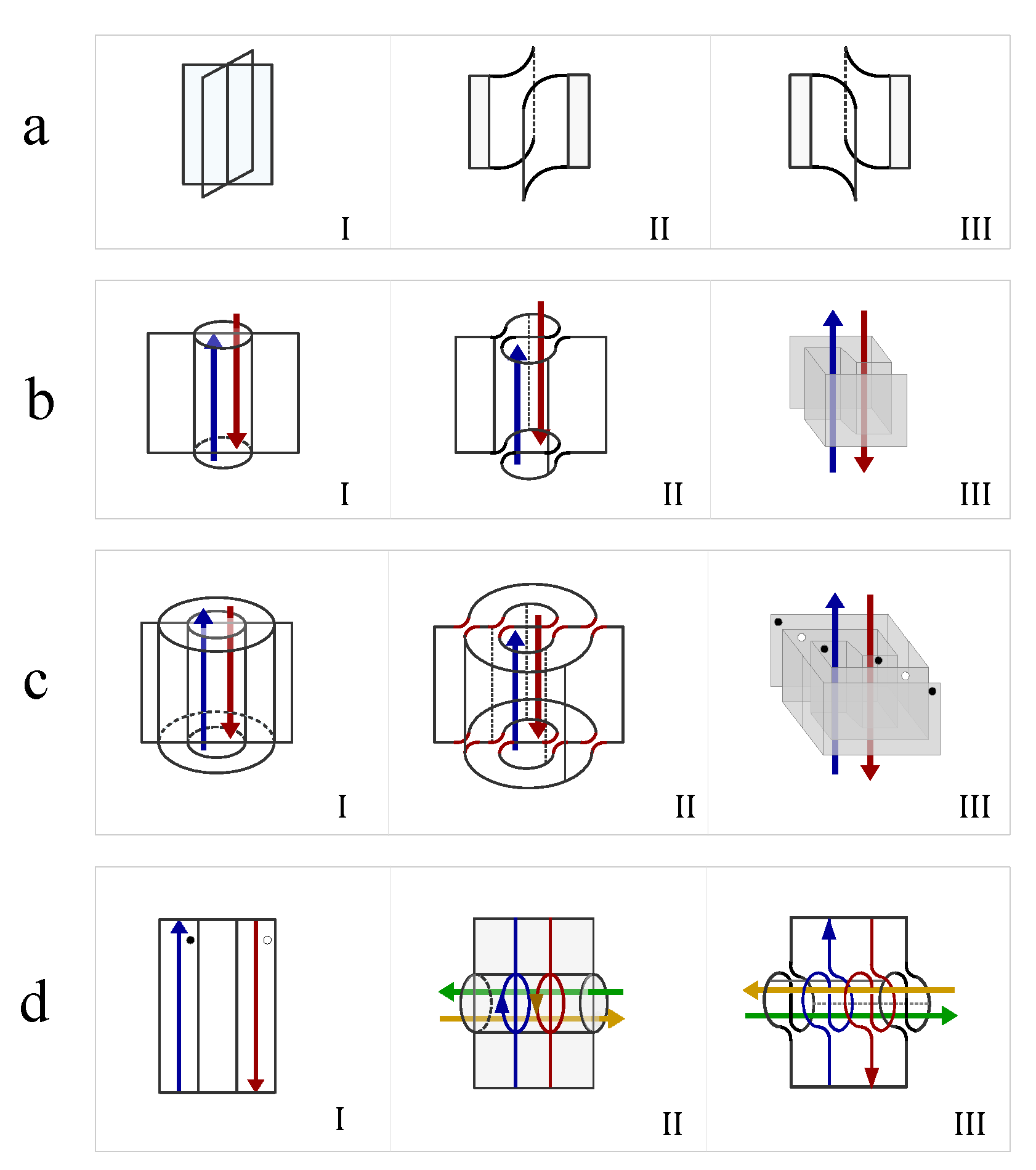
Figure 44.
(a) The explicit lamination pattern generated by braiding y- and fluxes once respectively is showed layer by layer. (b) The number of layers on the top and bottom side of magnetic fluxes are labeled by numbers. (c) The explicit lamination pattern generated by braiding y-fluxes twice and fluxes once. (d) The number of layers are distributed on top and bottom sides of interlocking magnetic fluxes in (c).
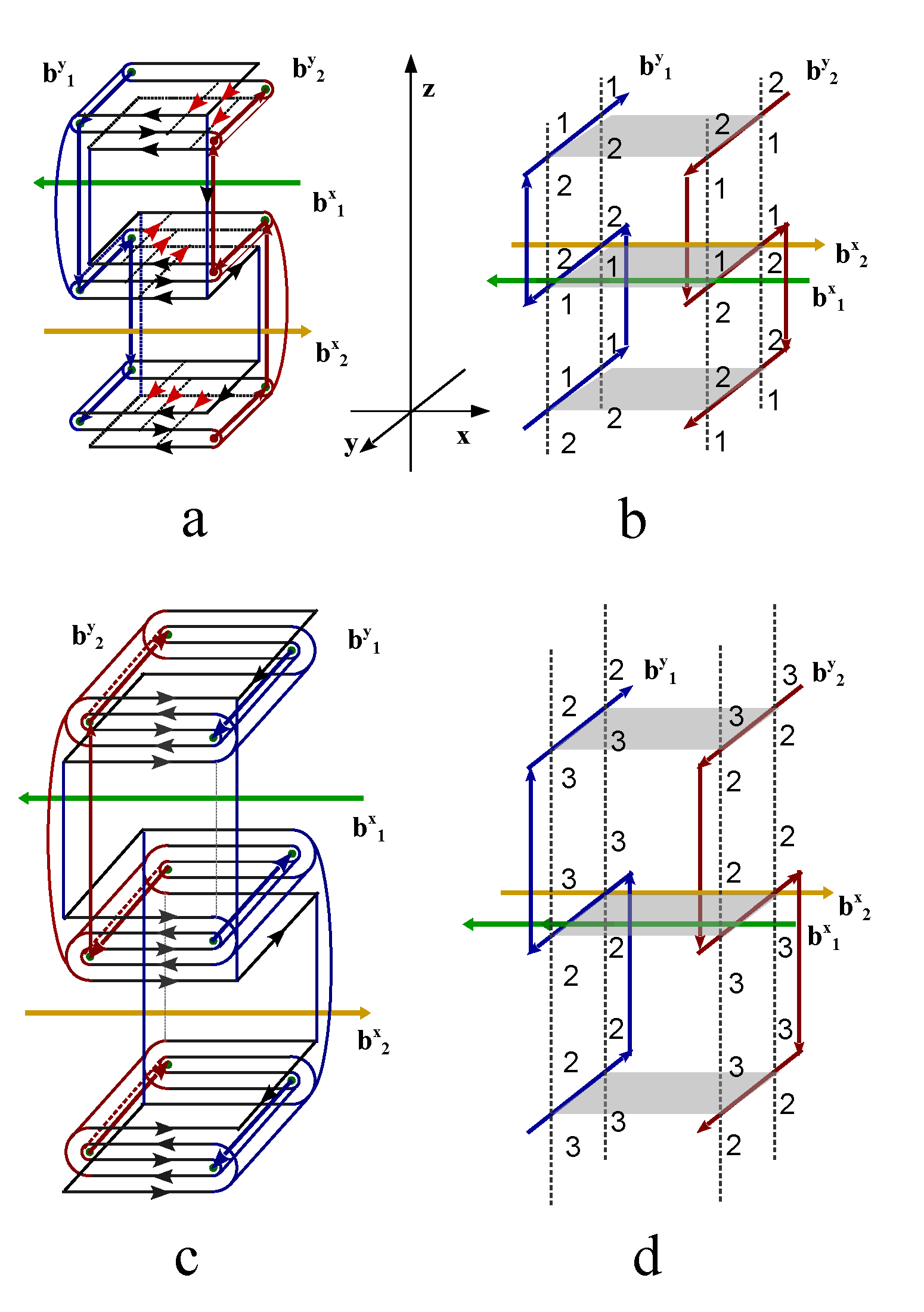
Figure 45.
(a) For an electric layer that only passes one side of the fluxes alternatively, braiding the three magnetic fluxes oriented in y-axis under two braidings, , generates a typical electric lamination. (b) Braiding a general initial lamination around three fluxes in x-axis under the braiding sequence , generates a stacked lamination.
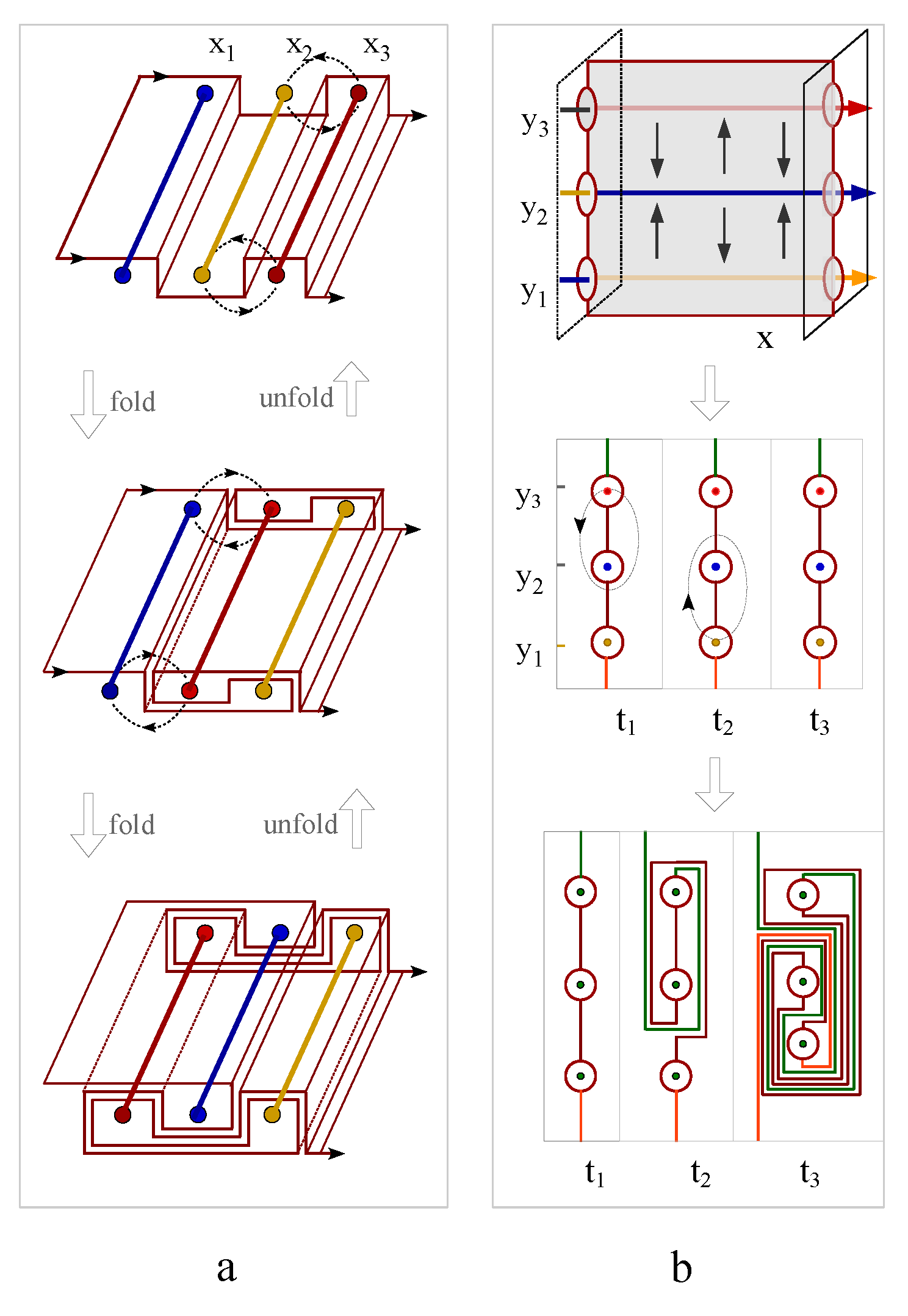
Figure 48.
(a) The genus array connects two laminar surfaces to create multi-connected space. (b) The two dimensional knot lattice in multi-connected space. (c) The intersecting tubular channels in three dimensional space. (d) The non-intersecting tubular surfaces envelopes three dimensional knot lattice of magnetic fluxes. (e) Braiding one flux with another one in tubular surface in y-axis folds the electric lamination. (f) Braiding two fluxes wrapped by two different tubular surfaces respectively folds the electric lamination.
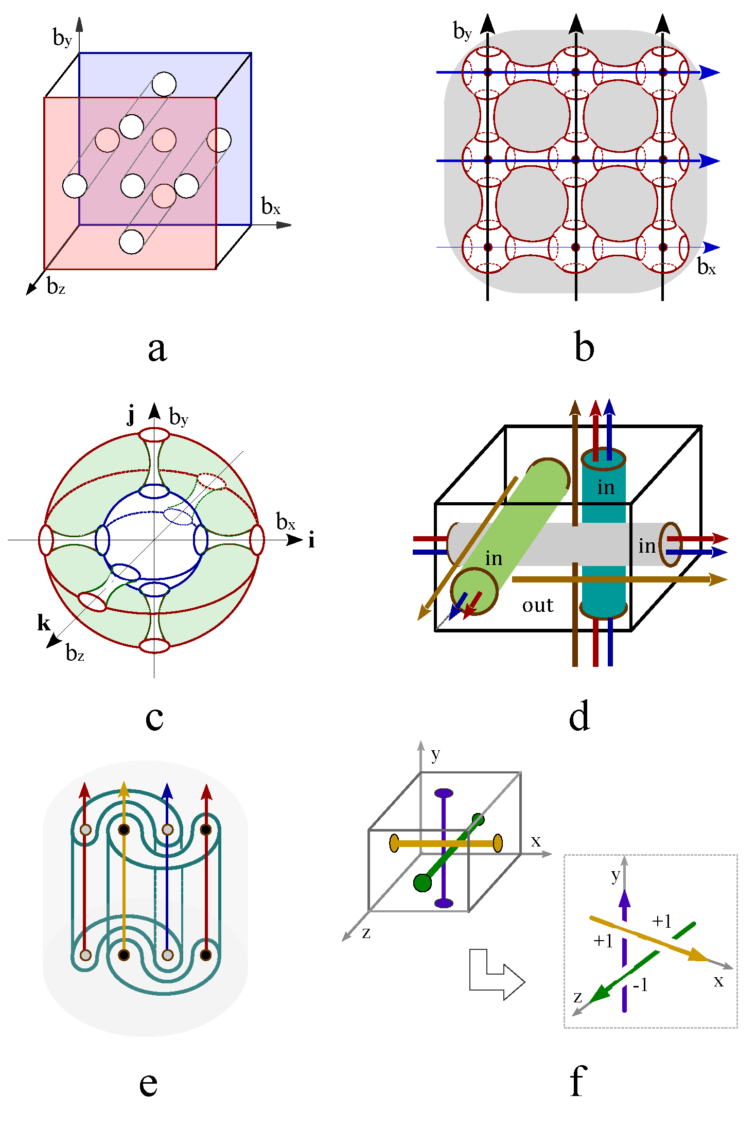
Figure 49.
(a) The topological representation of fermion with spin . (b) The topological representation of a pair of fermions with opposite spins in the same topological manifold of quantum states , visualizing Pauli exclusion principal. (c) The topological representation of many bosons distributed in three quantum states.
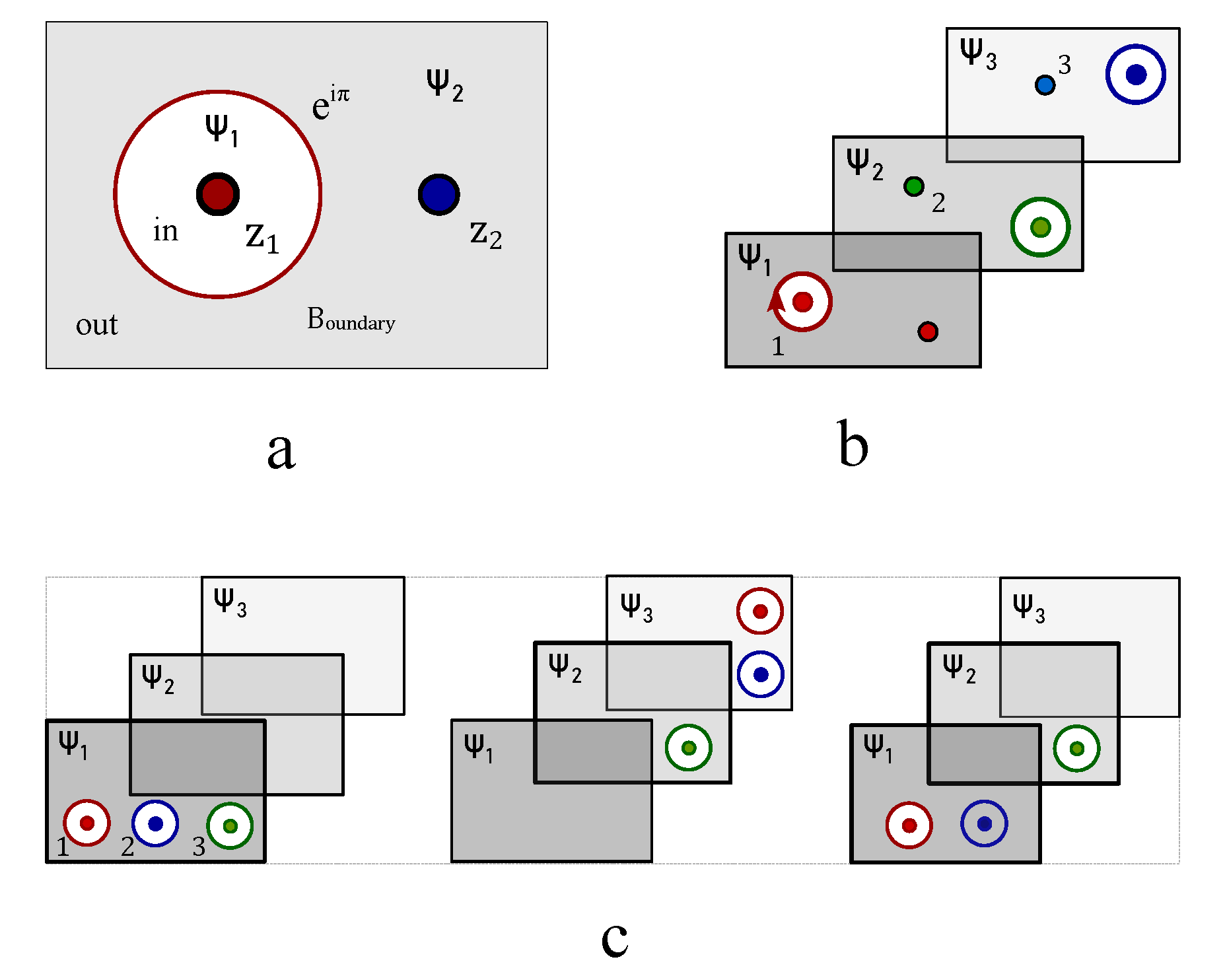
Figure 50.
(a) The fermions are divided by a phase boundary of . (b) The one dimensional boundary is expanded into a two dimensional cylindrical manifold. (c) Two anyons are separated by a boundary with a phase difference . (d) The boundary manifold between two anyons is a fan surface of cylinder that projects an angle . (e) The phase boundary of two bosonic fluids is tangent to the fluid surface, sweeping over an angle of m2 in (f).
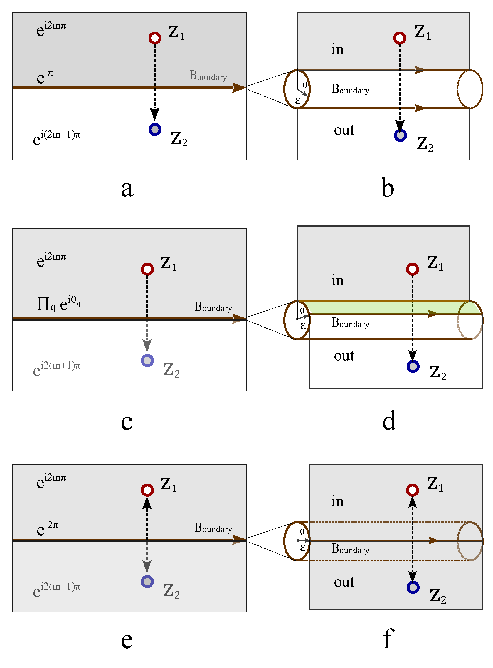
Figure 51.
(a) The fractional phases of anyons in two dimensions generated by braiding the two singular points in two opposite domains. (b) A clockwise rotation of the two singular points generates the spiral boundary pattern. (c) The spiral boundary fuse into one triple layer boundary segment. (d)(e) The two particles are braided in clockwise direction twice to generate a dual spiral boundary pattern, which folds into a triple layer boundary segment in (f). (g) Four particles in three different regions. (h) Braiding two particles and in clockwise direction. (i) The phase boundary among four particles are renormalized after braiding.
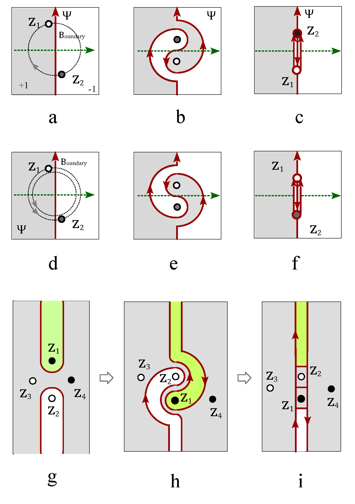
Figure 52.
(a) The three dimensional space is divided into two fermionic domains by an open boundary surface with . (b) Three dimensional compact manifold is divided into two separate compact domains by a two dimensional spherical surface, each of the compact domain confines singular point as a representation of point particle. (c) The blue point particle winds around the red point particle and return to its initial point, the close trajectory continuously contracts to the original point. (d) Three dimensional compact manifold is divided into two separate domains by a torus surface with one genus. (e) The boundary surface is a torus surface with 2-genus. (f) A multilayered concentric torus surface divide the three dimensional space into many isolated domains. (g) The torus boundary surface carries a statistical phase .
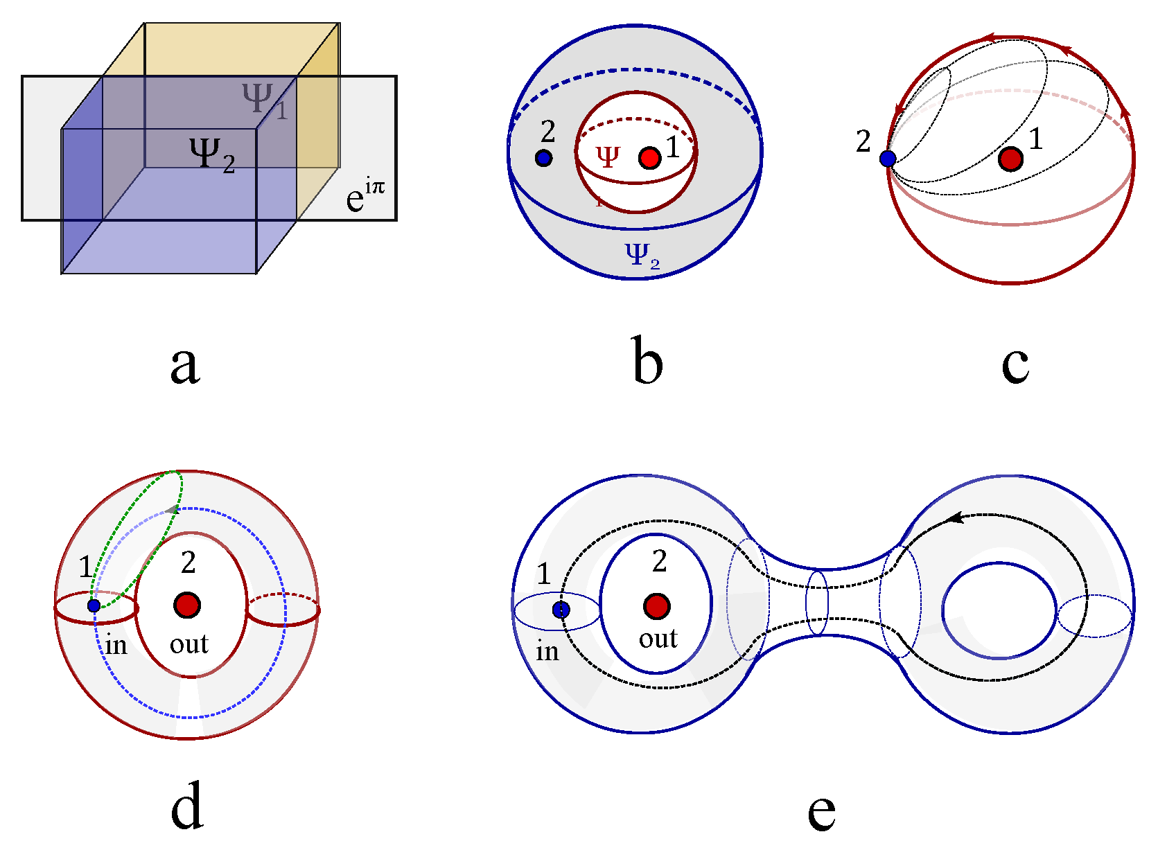
Figure 53.
(a) Two fermions are divided into two domains by a boundary surface with . The two fermions are braided around a horizontal axis in (b) and a vertical axis in (c). (d) The explicit nine layers of boundary surface that envelops the two particles. (e) Two particles are trapped in a stacked lamination under general braiding protocol.
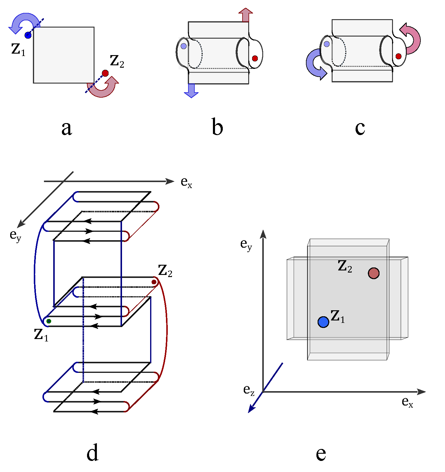
Figure 54.
(a) A singular loop is created by cutting one simple connected manifold into two domains. (b) A solid ball is cut into two concentric spherical shells, two spherical edges are created simultaneously to cover the singular spherical gap. (c) A tubular tunnel connects the inner and the outer spherical edge surface to fuse them into one. (d) Two tubular tunnel maps the two edge spheres into a torus with two genus. (e) Four tubular tunnels transform the two edge spheres into a torus with three genus.
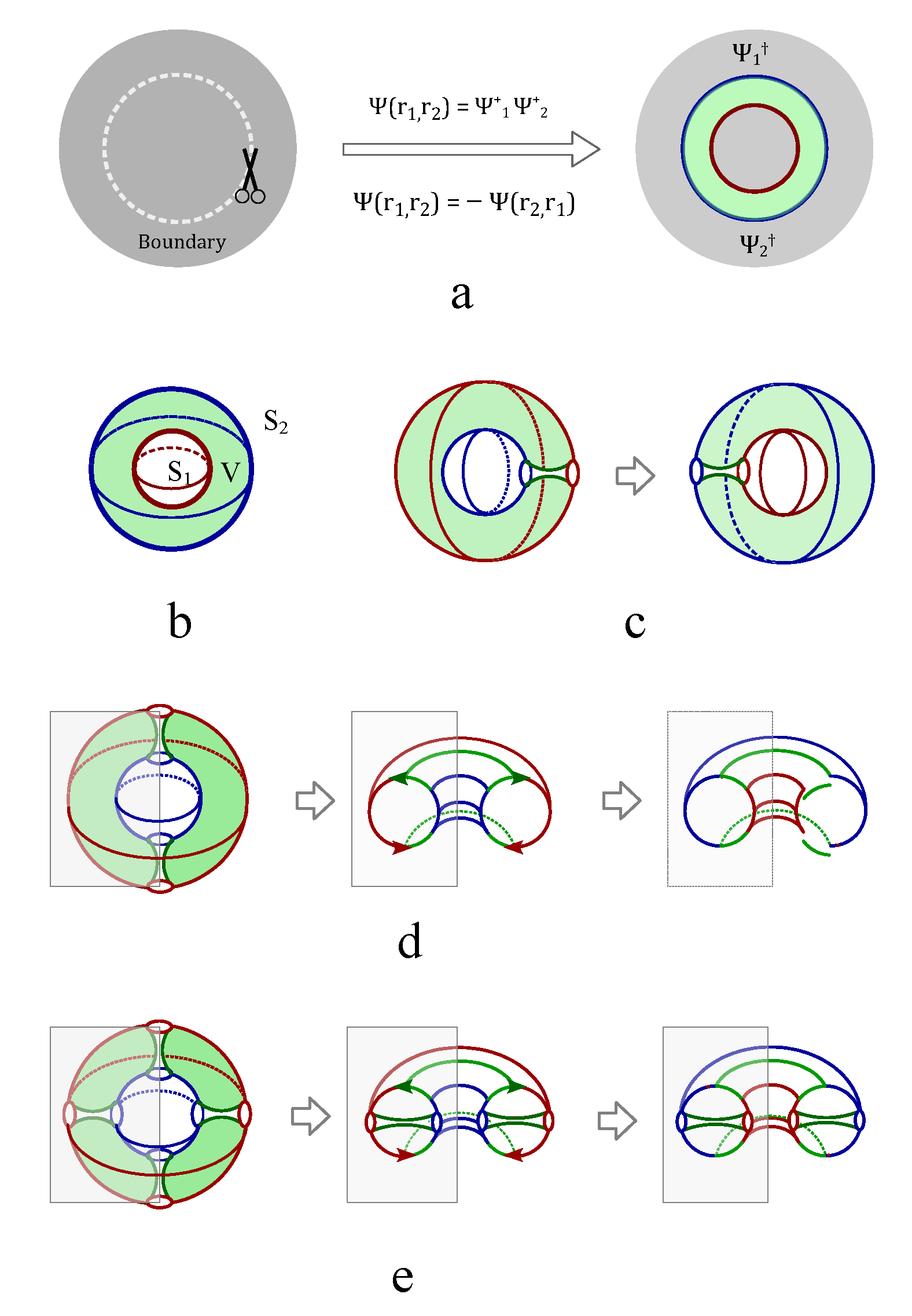
Figure 55.
(a) Four concentric magnetic flux loops are plugged in four concentric torus surfaces. (b) The four contacting points in the cross section on the right hand side of the multilayered torus are braided once and twice in (c). (d) The knot lattice of magnetic fluxes with respect to train track in (b). (e) The knot lattice of magnetic fluxes with respect to (c).
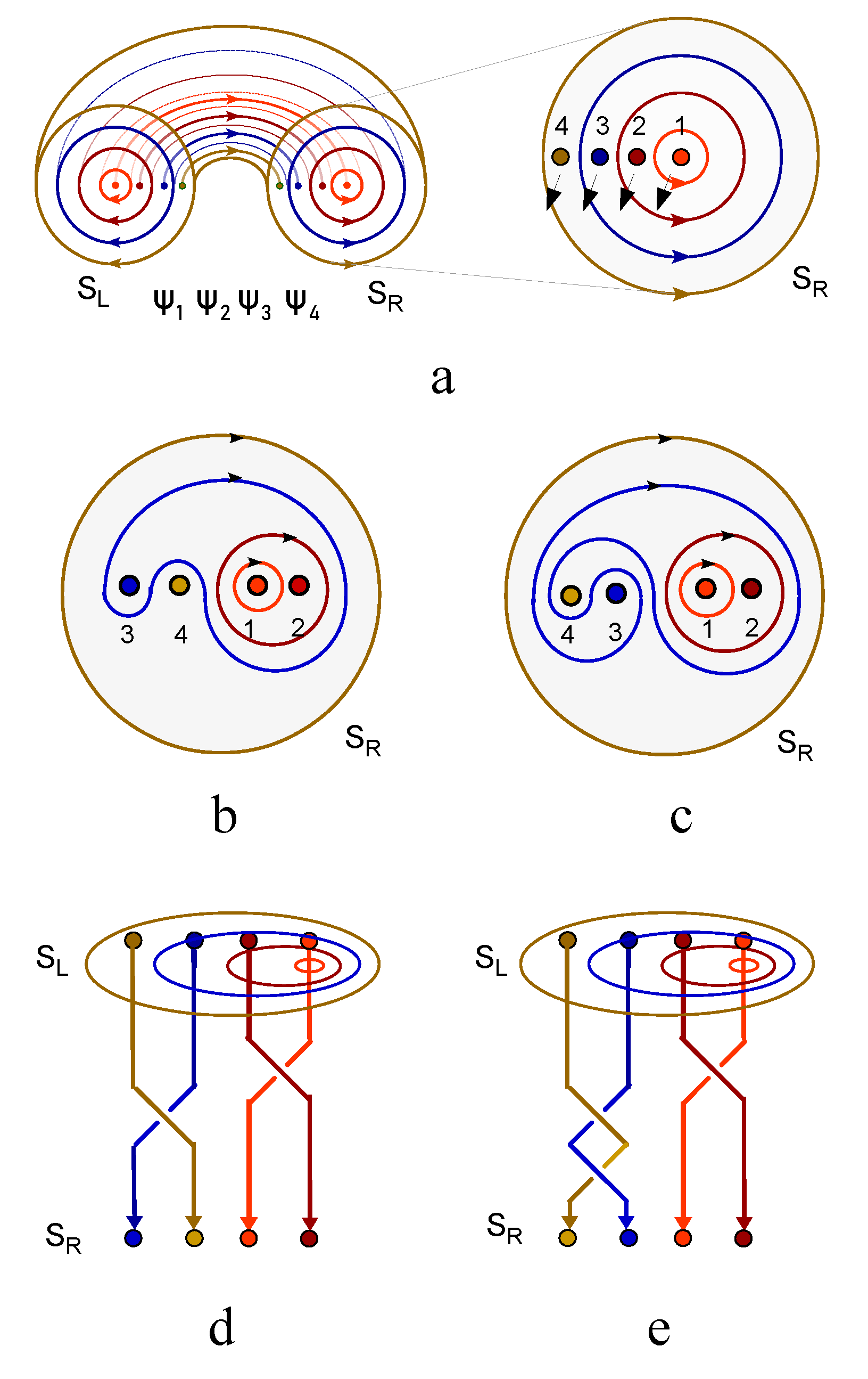
Figure 56.
(a) A spin chain formed a ring with two opposite crossings. (b) The deviation of spin from z-axis. (c) The effective potential landscape of a rotating spin in a continuous ribbon of electron fluid. The alternating knot ring formed by odd number of crossings in (d) and even number of crossings in (e). (f) Flipping a local spin from to generates the knot ring with crossings.
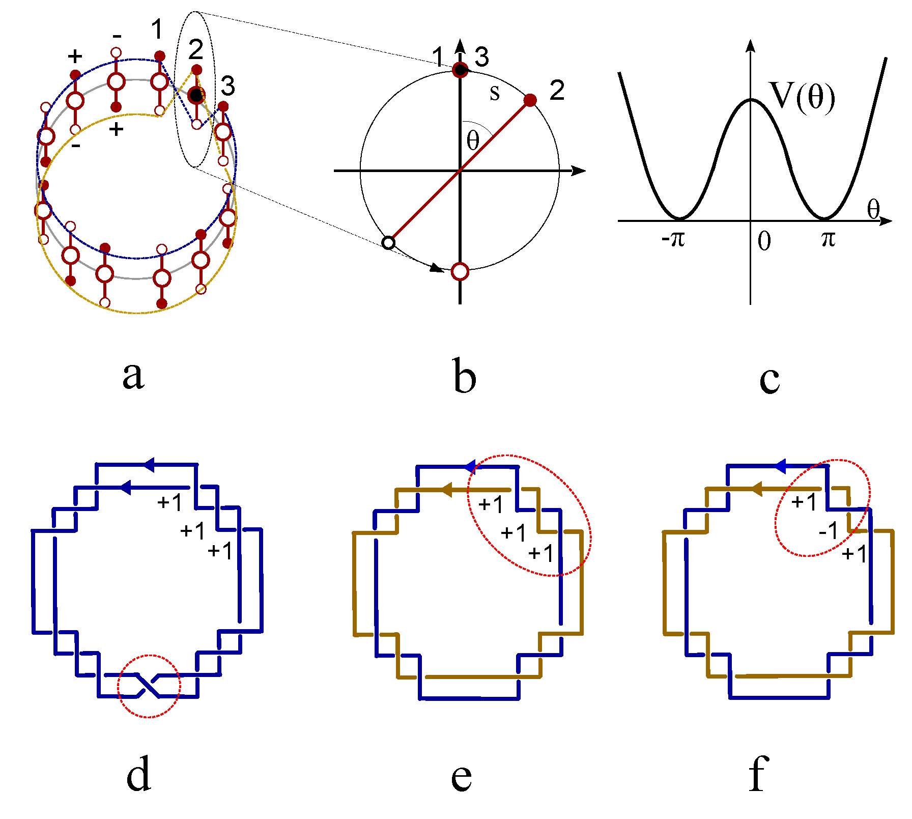
Figure 57.
The von Neumman entropy of torus knot with the right-hand crossings (indicated by the blue curve) drops to zero at zero temperature. The entropy of the left-hand torus knot (the red curve) drops to zero at finite temperature.
Figure 57.
The von Neumman entropy of torus knot with the right-hand crossings (indicated by the blue curve) drops to zero at zero temperature. The entropy of the left-hand torus knot (the red curve) drops to zero at finite temperature.
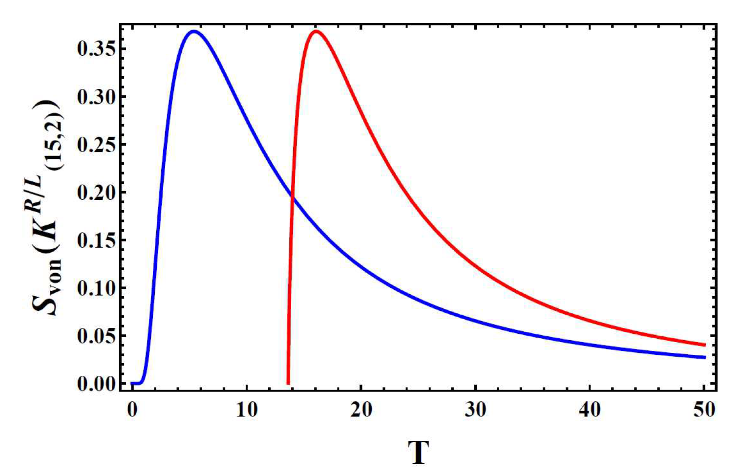
Figure 58.
The decaying of von Neumman entropy of torus knot with the right-hand crossings (indicated by the blue curve) at low temperature (dimensionless).
Figure 58.
The decaying of von Neumman entropy of torus knot with the right-hand crossings (indicated by the blue curve) at low temperature (dimensionless).
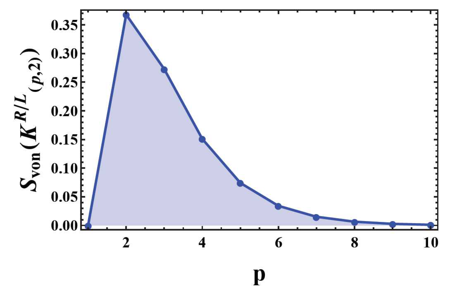
Figure 59.
The decay of von Neumman entropy of torus knot with the right-hand crossings (indicated by the blue curve) and the left-hand cross (the red curve) at intermediate temperature (dimensionless) .
Figure 59.
The decay of von Neumman entropy of torus knot with the right-hand crossings (indicated by the blue curve) and the left-hand cross (the red curve) at intermediate temperature (dimensionless) .
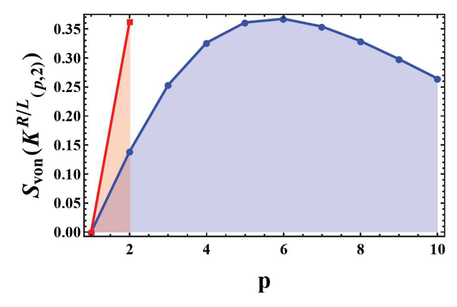
Figure 60.
The decay of von Neumman entropy of torus knot with the right-hand crossings (indicated by the blue curve) and the left-hand cross (the red curve) at high temperature (dimensionless).
Figure 60.
The decay of von Neumman entropy of torus knot with the right-hand crossings (indicated by the blue curve) and the left-hand cross (the red curve) at high temperature (dimensionless).
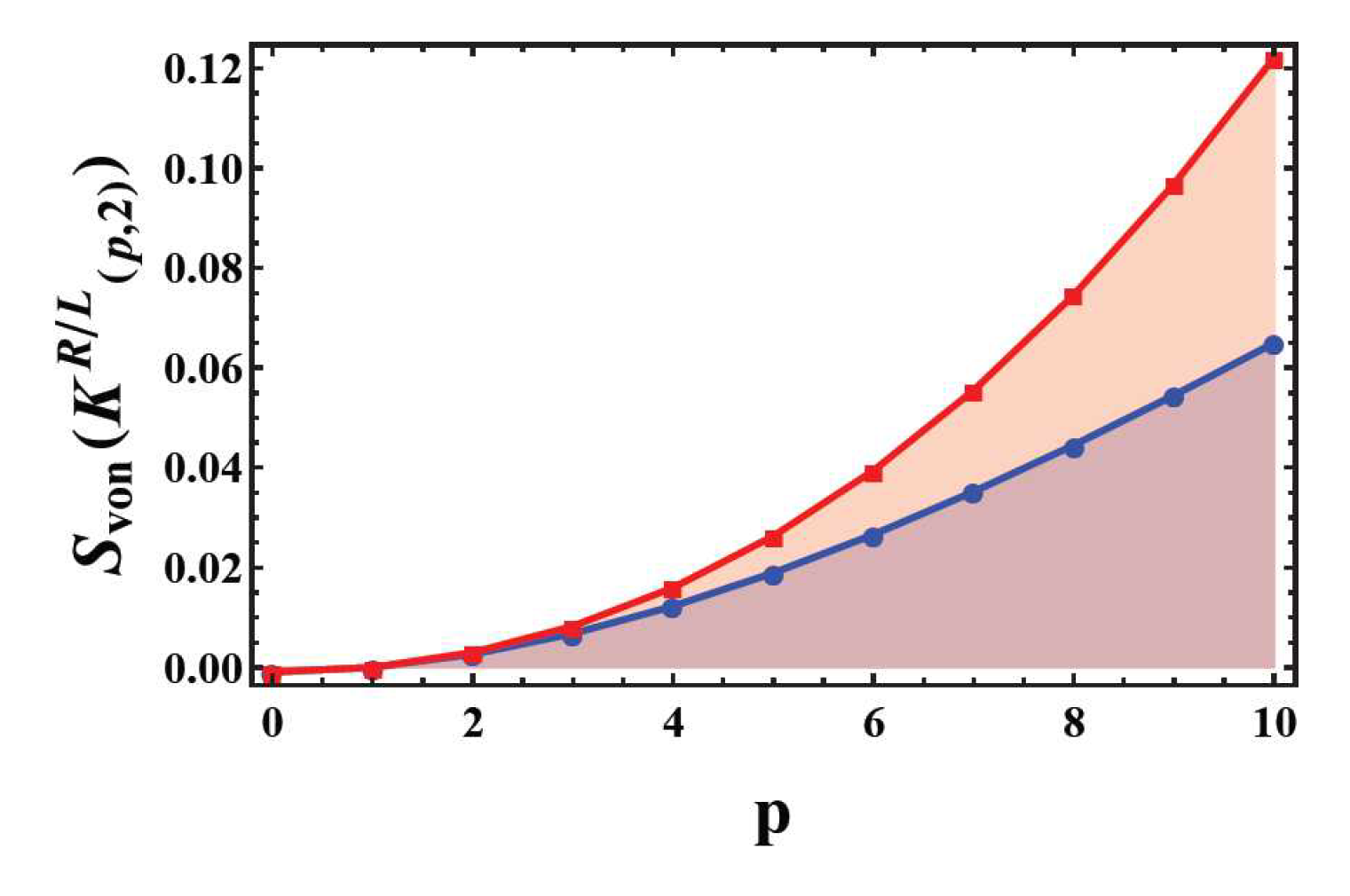
Figure 61.
(a) The knot lattice covered by Seifert surface. (b) One crossing (indicated by the blue dashed circle) transforms into an uncrossing state , and (c) the other uncrossing state . (d) Two knot genus fuse into one big genus. (e) The chiral spin liquid is represented by lattice fluid covered by fermionic dimers. (f) The superfluid state is represented by topological fluid of bosonic dimers.
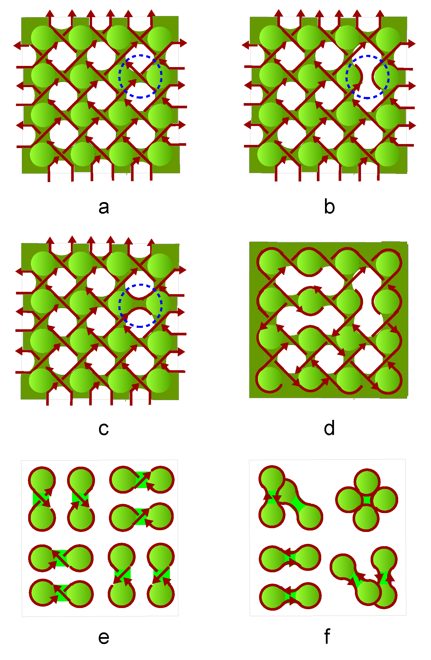
Figure 62.
(a)(b) The angle between the top current and the bottom current of crossing No. 1 is denoted as . (c) The continuous variation of angle in the left-handed vacuum state. (d) The square lattice covered by full vacuum states and a global vacuum state in (e). (f) Two dimensional square lattice of knots. (g) The square lattice covered by a general knot crossing pattern.
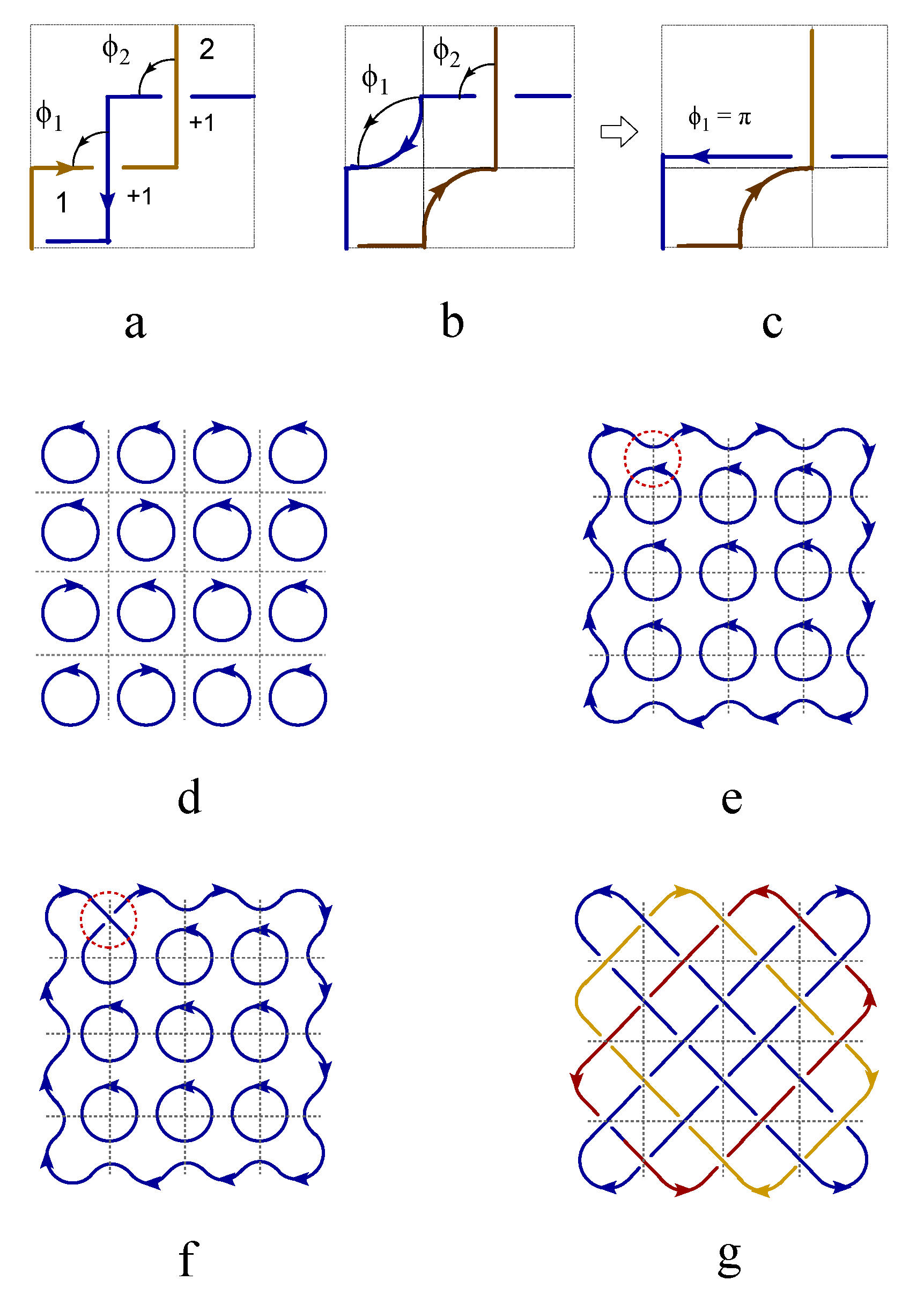
Figure 63.
(a) The square lattice constructed by intersecting electron fluid ribbon. (b) The equivalent mapping of twisted electron ribbon into knot lattice of magnetic loops. (c) The toric code model of interacting spins. (d) The chirality flips under the action of four spin operators.
Figure 63.
(a) The square lattice constructed by intersecting electron fluid ribbon. (b) The equivalent mapping of twisted electron ribbon into knot lattice of magnetic loops. (c) The toric code model of interacting spins. (d) The chirality flips under the action of four spin operators.
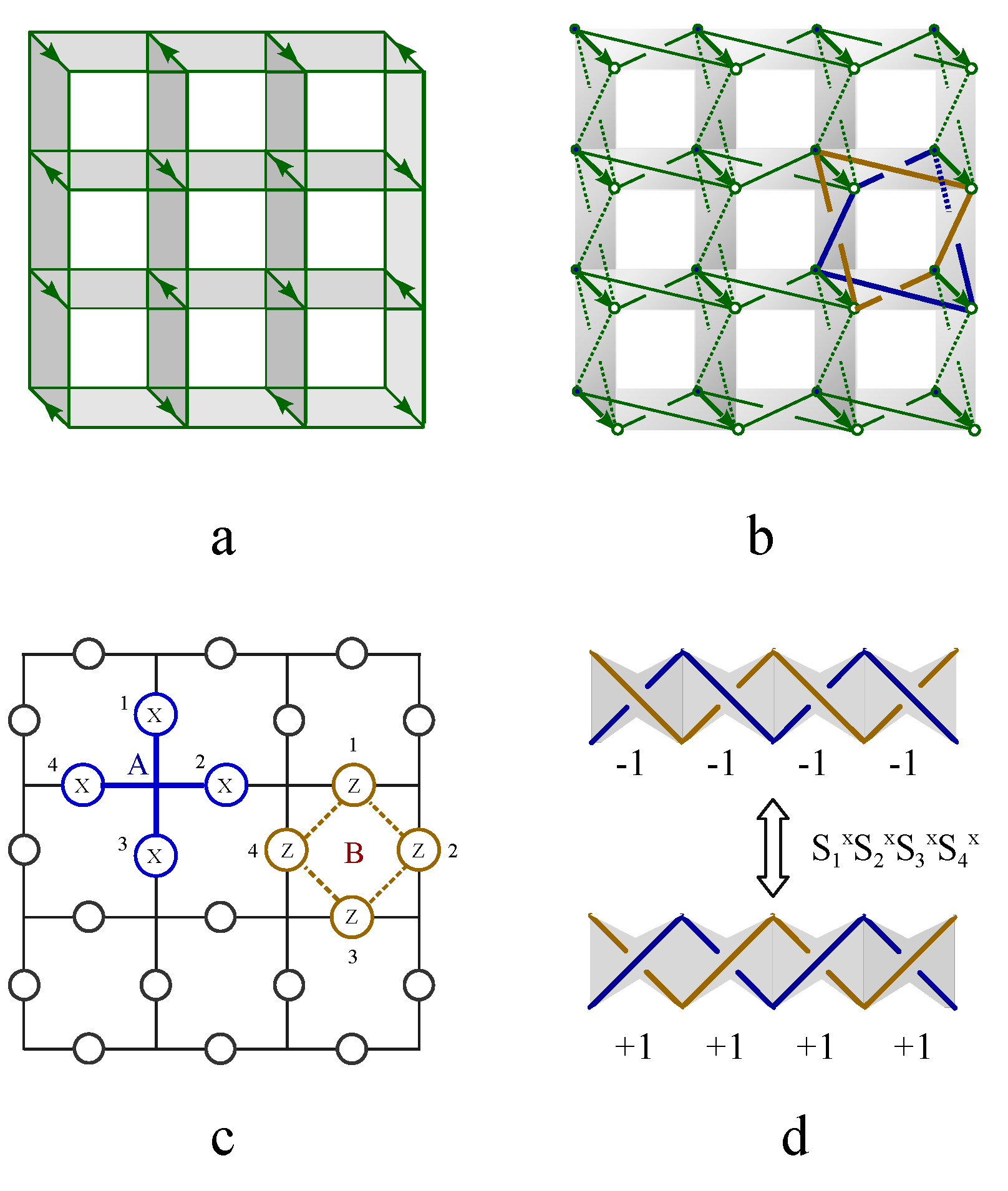
Figure 64.
(a) The two intersecting electron fluid ribbons are projected into a composite knot composed of four crossings. (b) The knot pattern representation of four interacting spins at the four corner of square.
Figure 64.
(a) The two intersecting electron fluid ribbons are projected into a composite knot composed of four crossings. (b) The knot pattern representation of four interacting spins at the four corner of square.
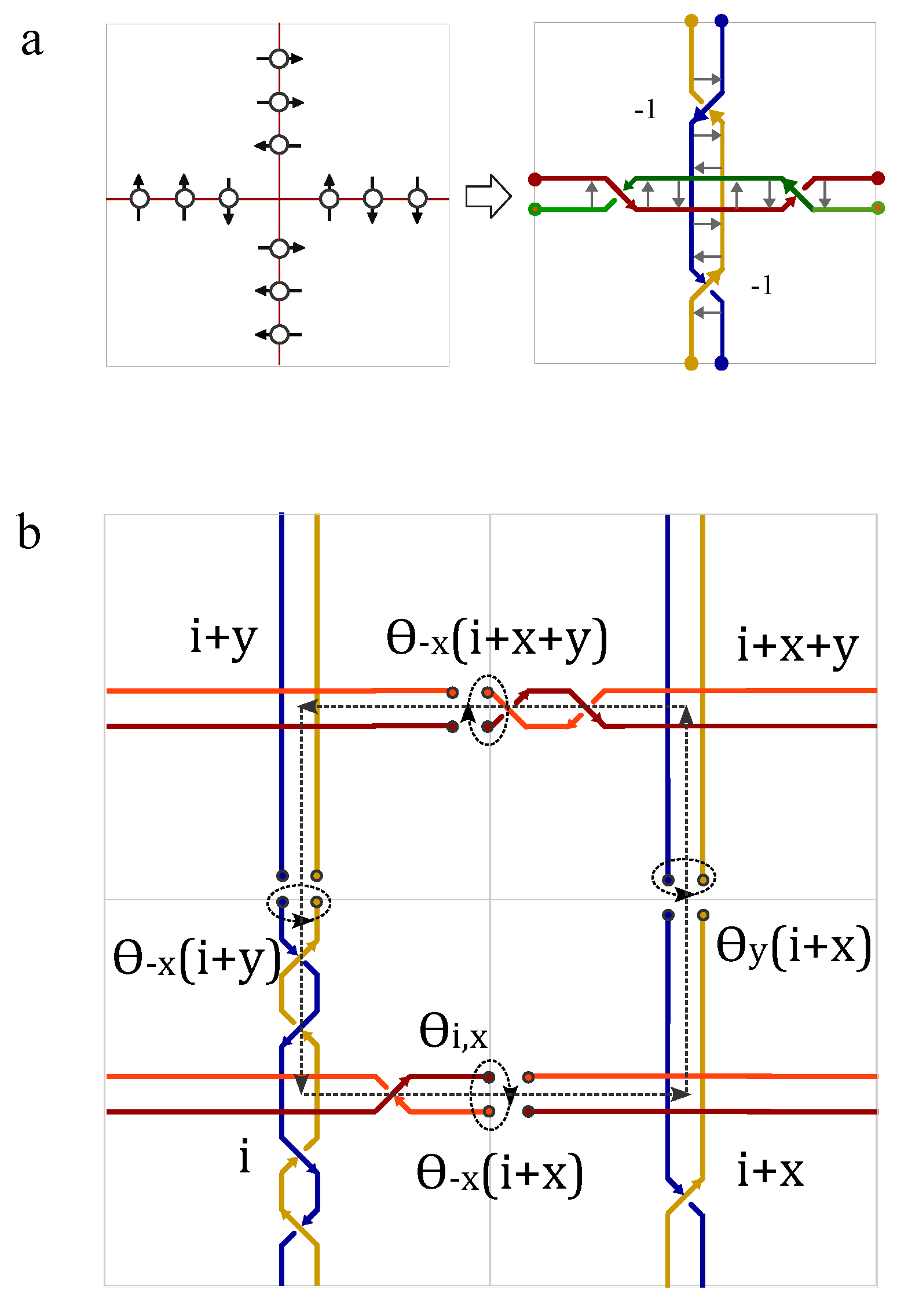
Figure 65.
(a) The two dimensional knot lattice representation of four double crossings. (b) The topological representation of the one dimensional edge of knot lattice with crossing-avoiding boundary condition.
Figure 65.
(a) The two dimensional knot lattice representation of four double crossings. (b) The topological representation of the one dimensional edge of knot lattice with crossing-avoiding boundary condition.
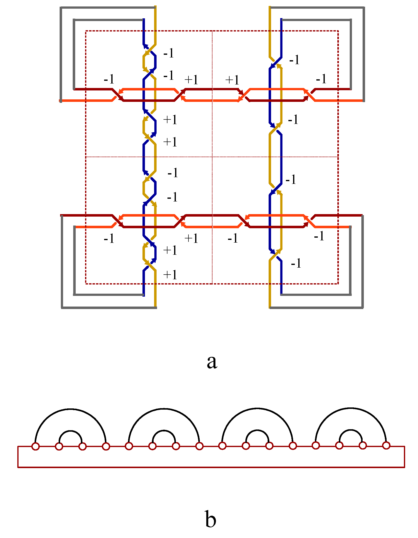
Figure 66.
(a) A free topological spin represented by a free crossing moving at speed of . (b) A free crossing moves along a folded path in magnetic field. (c) The two endings of open fluid strip unit to form a Mbius strip. (d) Two opposite spins paired up to form a flat strip. (e) The thermal de Broglie wavelength of a circular fluid covers over a finite disc area. (f) The fluid loops that represent topological spins enlarges to squeeze and overlap one anther when temperature drops. The black open track represents free topological spins. (g) Two nearest neighboring Mbius strips paired up to form a dimer. The dimer covering of square lattice is superconductor state.
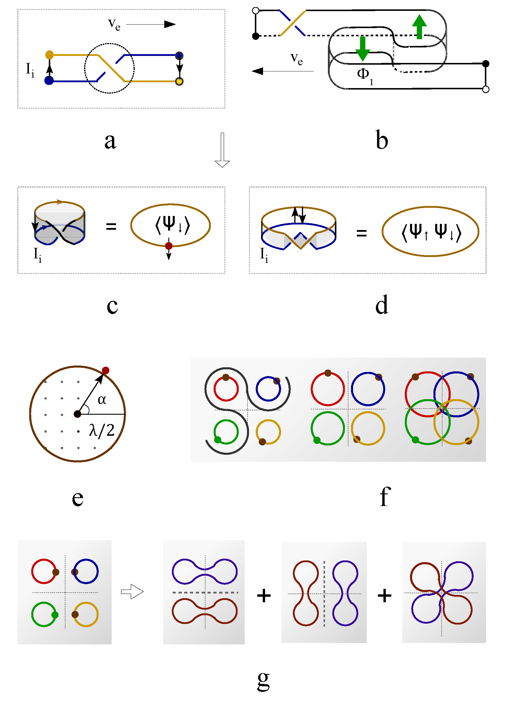
Figure 67.
(a) The dimer covering of square lattice by flat strip loops. (b) The flat strip loop is mapped into a finite line segment with two endings. (c) The loops of Cooper pairs expand and fold into train tracks when temperature drops. (d) The elongated dimers wind around one another to form topological defect within superfluid. (e) The topological loop of dimer gains more degree of freedom to expand on lattice with lower filling factor.
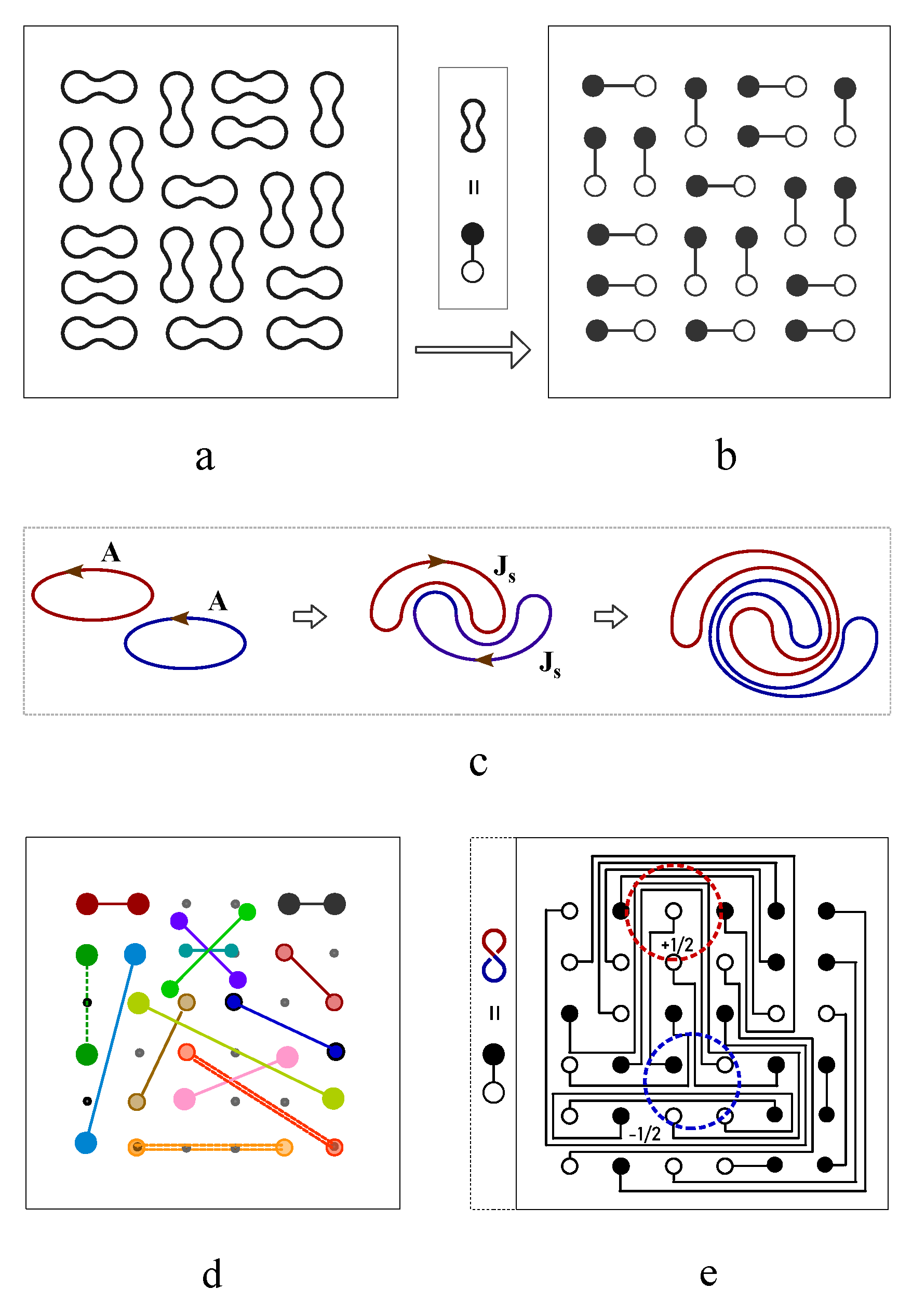
Figure 68.
(a) The two dimers with even number of crossings is topologically equivalent to the non-crossing configuration. (b) Two winding dimers with odd number of crossings are topologically equivalent. (c) The trains track in three dimensions generated by two braiding two finite dimers is topologically equivalent to the unwinding track. (d) The train track generated by an odd number of braiding in three dimensions are topologically equivalent.
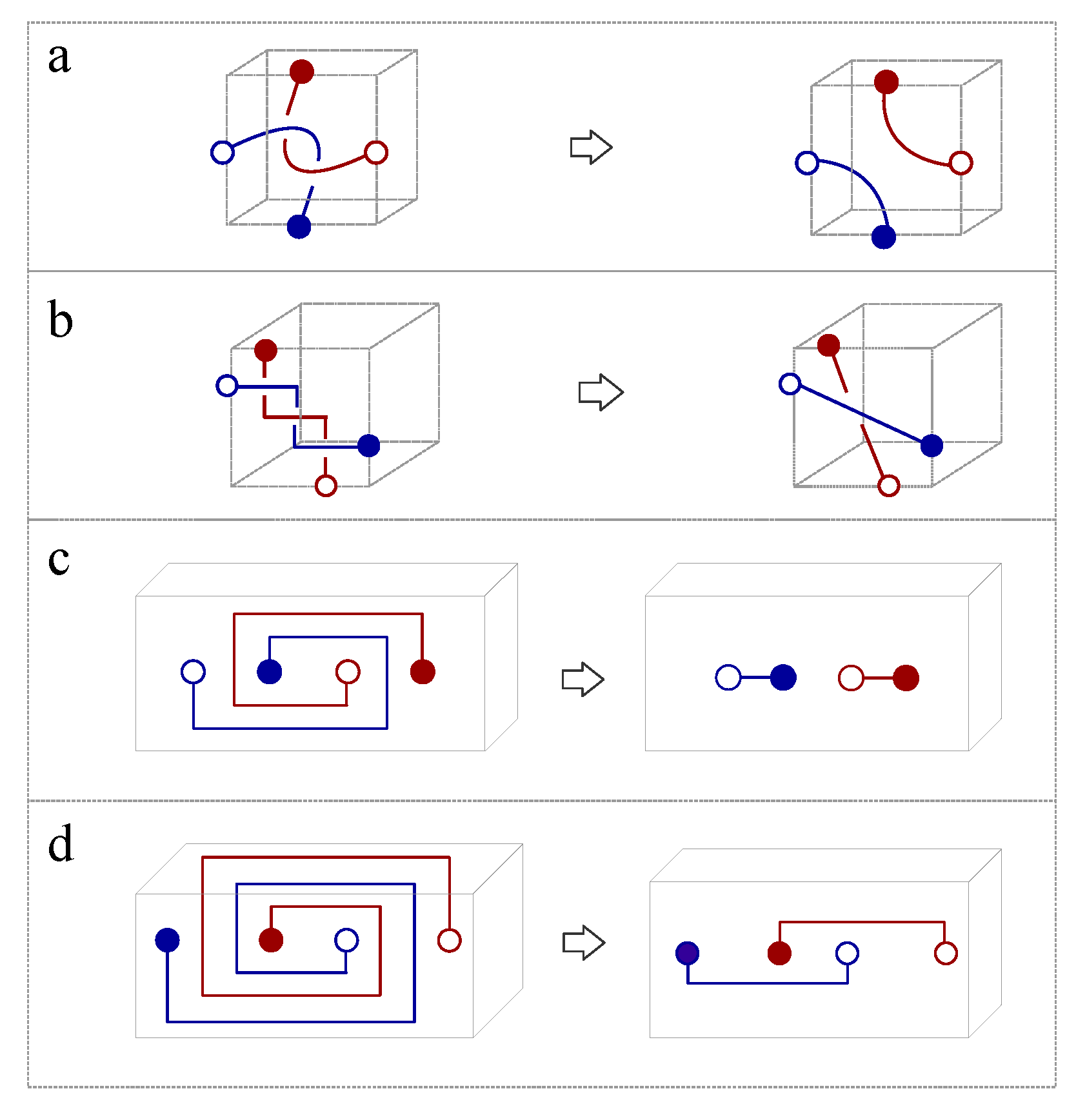
Figure 69.
(a) Opposite spins paired up to form quantum fluid loops of Cooper pair, as representation of s-wave superconductor. (b) In d-wave superconductor, the energy gap of superconducting phase closes along the dislocation line in (c) to form a gapless nodal line under topological translation and reconnection.
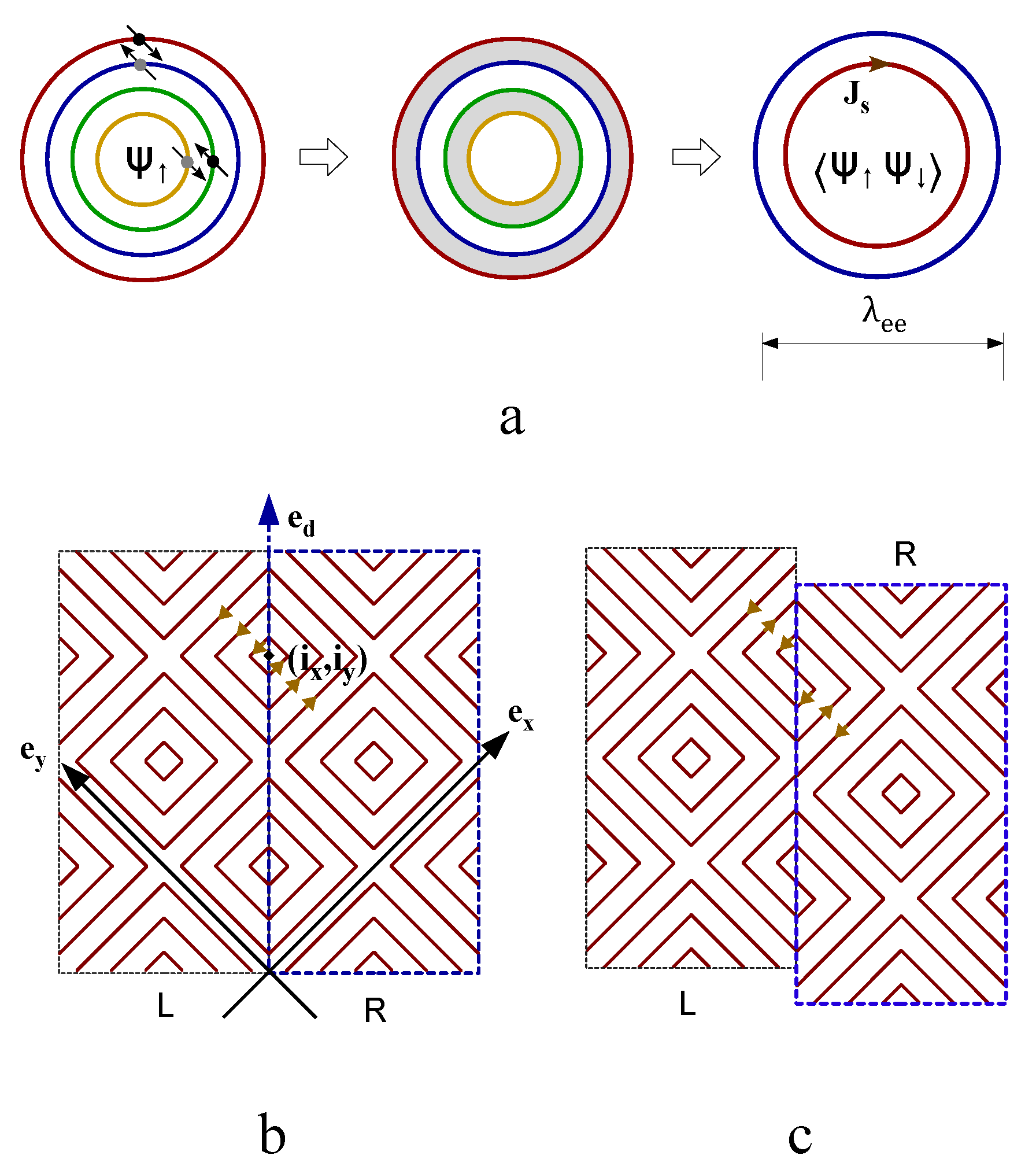
Figure 70.
(a) The Feynman diagram of one dimensional chain of Cooper pairs. (b) The Feynman diagram of Cooper pair in momentum space. (c) The Mbius strips representation of fermion with spin 1/2. (d) The Feynman diagram of pairing up two Mbius strips.
Figure 70.
(a) The Feynman diagram of one dimensional chain of Cooper pairs. (b) The Feynman diagram of Cooper pair in momentum space. (c) The Mbius strips representation of fermion with spin 1/2. (d) The Feynman diagram of pairing up two Mbius strips.
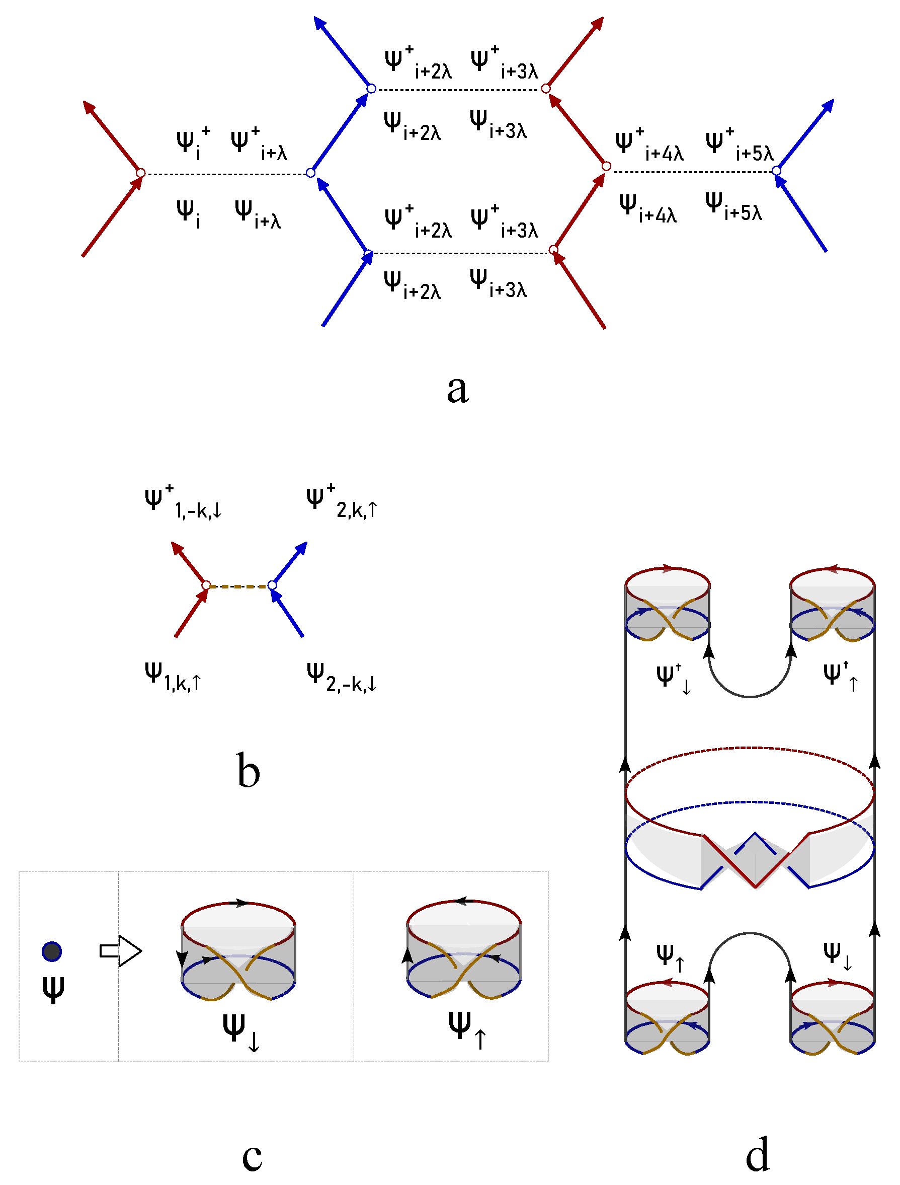
Figure 71.
(a) The Feynman diagram of Cooper pair annihilation and creation. (b) The decomposition of four-fermion product operator of Cooper pairs into quadratic forms of two creation operator multiplied by a gap function. (c) The decomposing of four-fermion product operator into electron-hole pair. (d) The intersecting point with four branches are untied as two lines avoiding crossing in pant diagram. (e) The chiral crossing is isolated from a knot lattice, the grey annulus represent the rest part of the knot lattice.
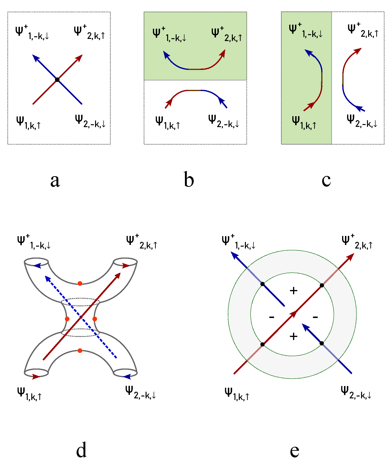
Figure 72.
(a) The topological equivalent strip representation of Cooper pair. (b) The topological strip of pairing up two identical spins. (c) The topological representation of spin angular momentum . (d) The Mbius strip is created by topological surgery on Klein bottle manifold. (e) Decomposition of knot crossing into vacuum state following Kauffman rule.
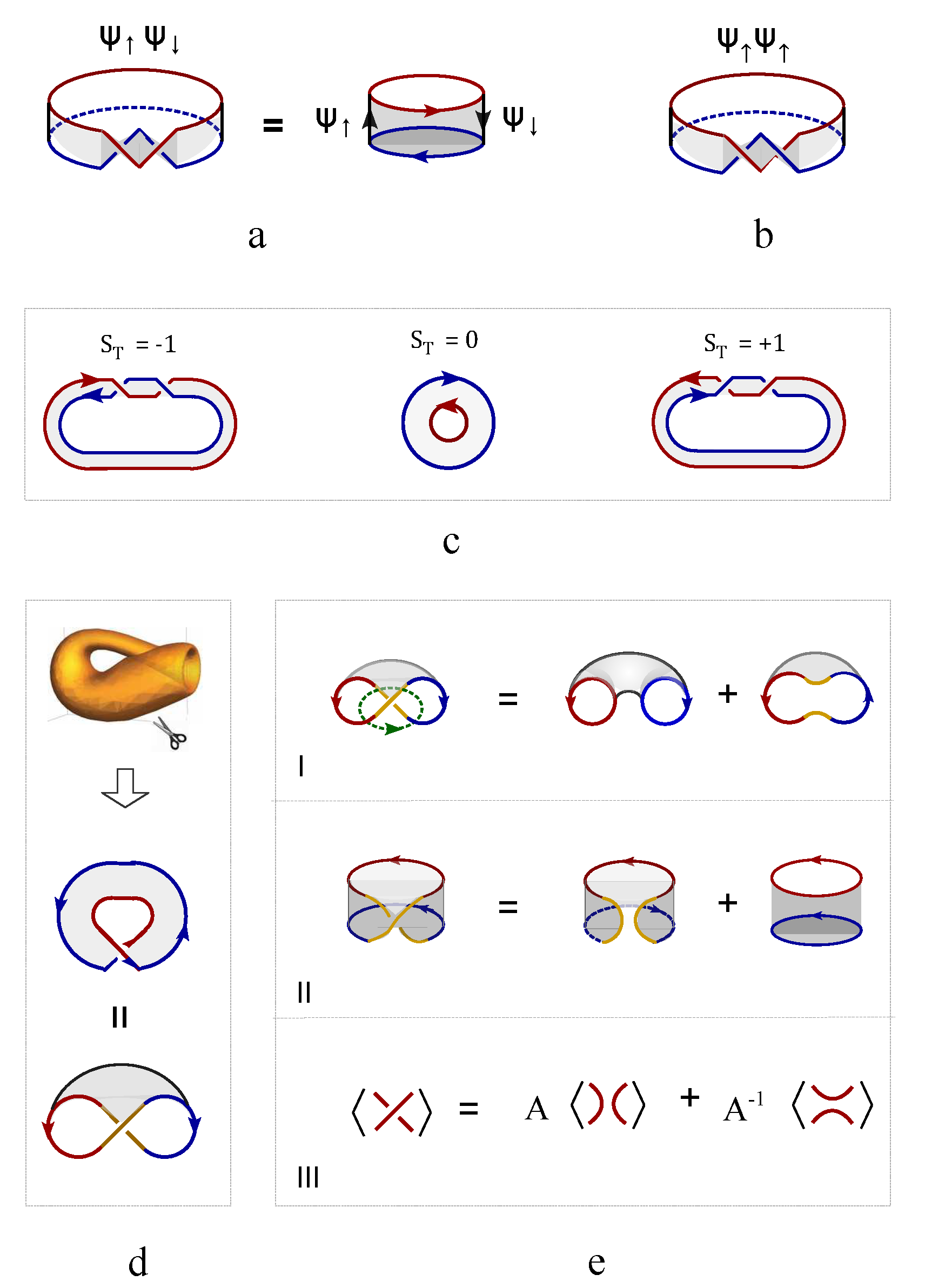
Figure 73.
(a) The sphere transforms into a disc by cutting a hole and a pair of discs by two cuttings. (b) The Feynman diagram of annihilating and creating a pair of rectangular membranes. (c) The tube representation of Cooper pair is created by cutting torus. (d) The pants Feynman diagram of the Cooper pairs.
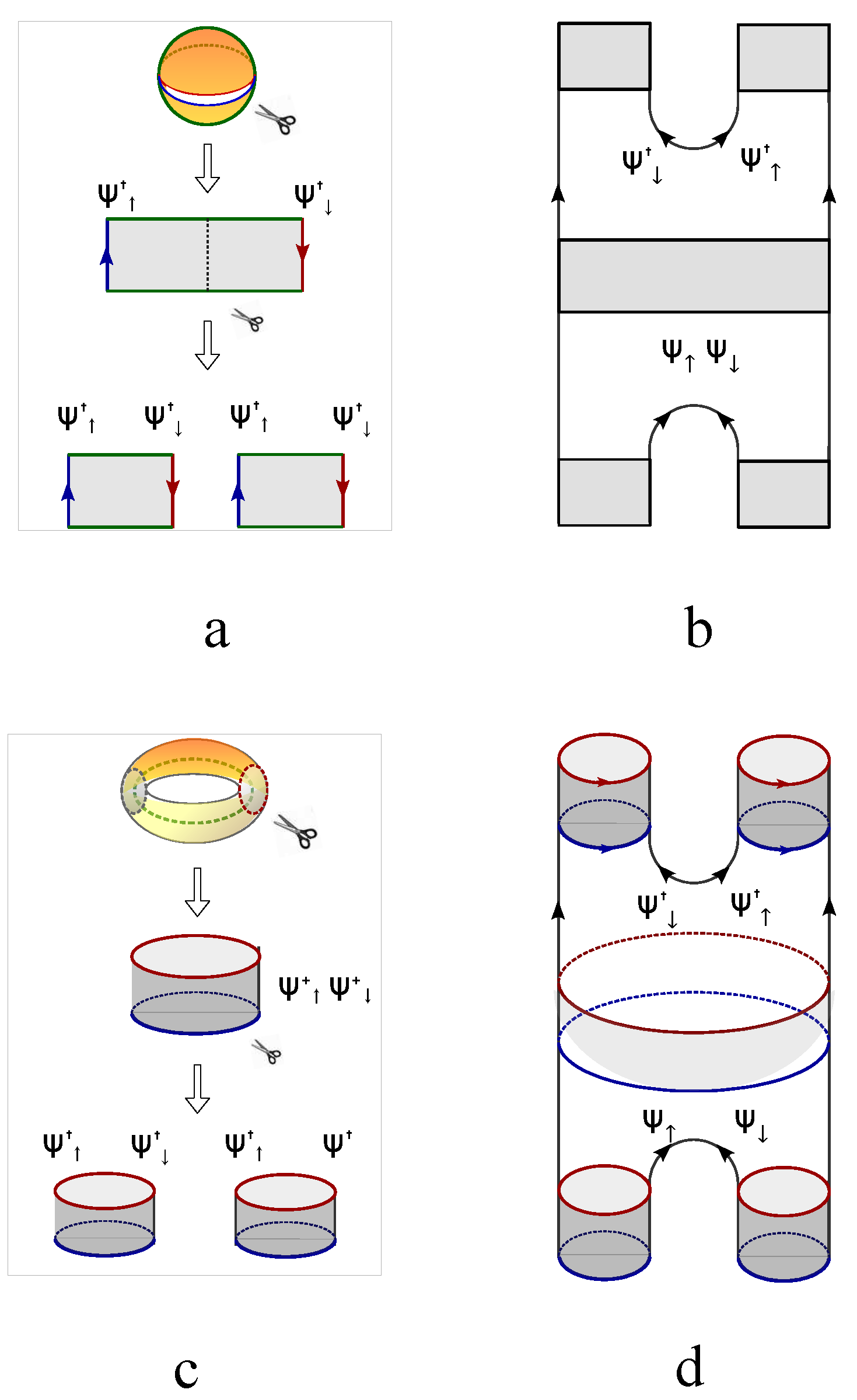
Figure 74.
The boundary conditions for constructing (a) Klein bottle, (b) sphere and (c) torus from knot square lattice. (d) The generalization of Kauffman decomposition rule of knot to that for two dimensional manifolds.
Figure 74.
The boundary conditions for constructing (a) Klein bottle, (b) sphere and (c) torus from knot square lattice. (d) The generalization of Kauffman decomposition rule of knot to that for two dimensional manifolds.
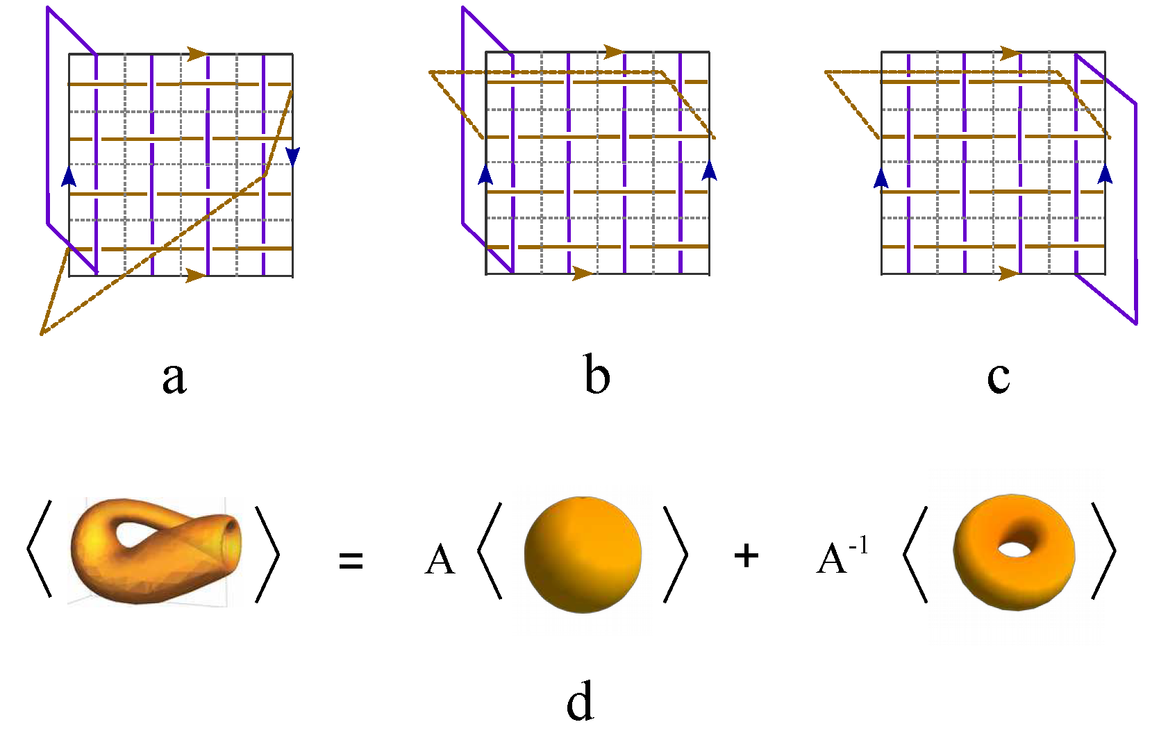
Figure 75.
The energy gap of electron hole pair varies with the occupation number of electron. The radius of the semicircular arc (the blue, the red, the green and the pink) is proportional to occupation number ( respectively).
Figure 75.
The energy gap of electron hole pair varies with the occupation number of electron. The radius of the semicircular arc (the blue, the red, the green and the pink) is proportional to occupation number ( respectively).
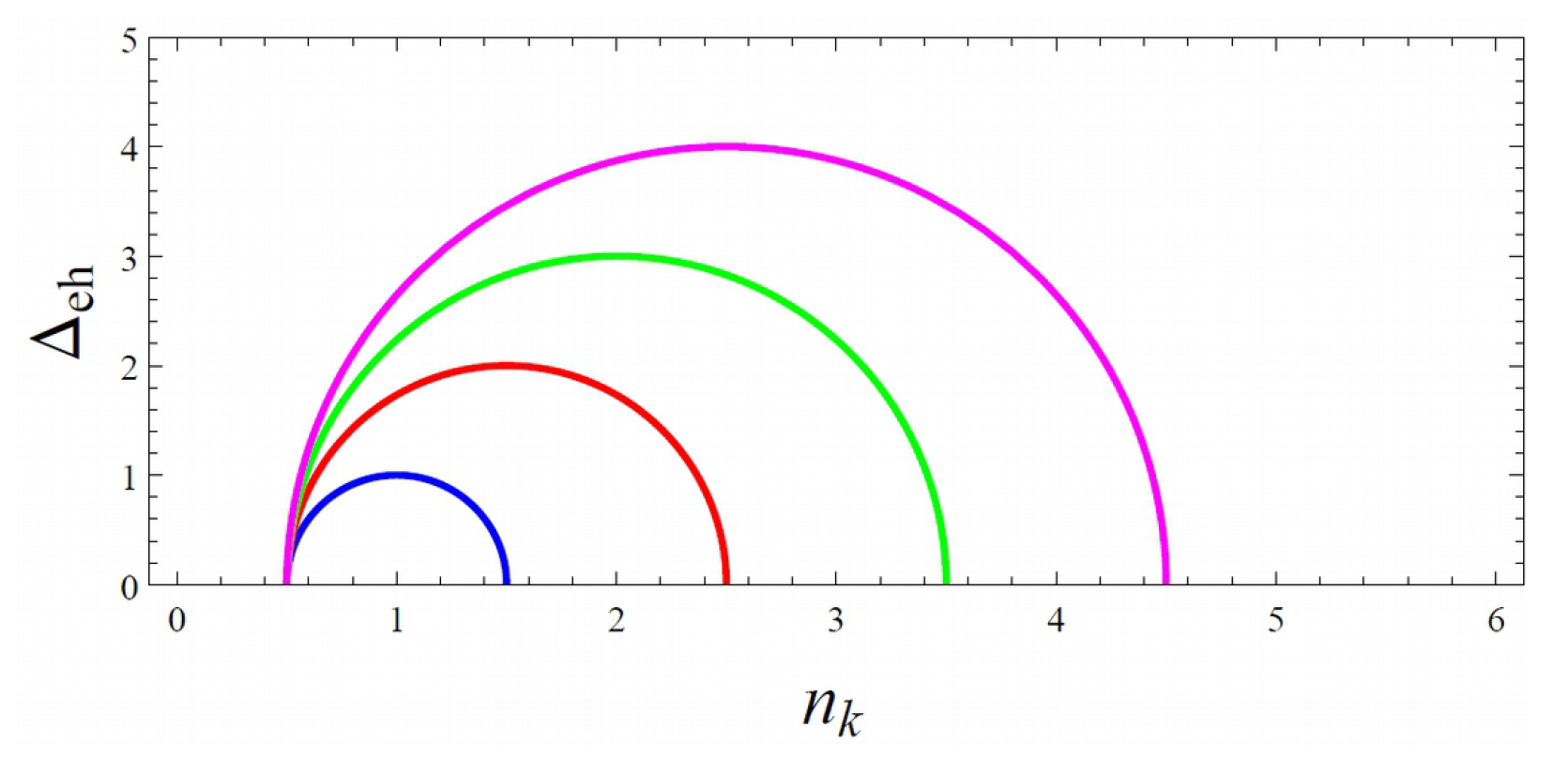
Disclaimer/Publisher’s Note: The statements, opinions and data contained in all publications are solely those of the individual author(s) and contributor(s) and not of MDPI and/or the editor(s). MDPI and/or the editor(s) disclaim responsibility for any injury to people or property resulting from any ideas, methods, instructions or products referred to in the content. |
© 2024 by the authors. Licensee MDPI, Basel, Switzerland. This article is an open access article distributed under the terms and conditions of the Creative Commons Attribution (CC BY) license (http://creativecommons.org/licenses/by/4.0/).
Copyright: This open access article is published under a Creative Commons CC BY 4.0 license, which permit the free download, distribution, and reuse, provided that the author and preprint are cited in any reuse.


