
Submitted:
23 July 2024
Posted:
24 July 2024
You are already at the latest version
Abstract
The origin and climate impact of Arctic aerosols, like the Arctic Haze, are not fully understood. Therefore, long-term aerosol observations in the Arctic are performed. In this study we present a homogenised data set from sun and star photometer operated in the European Arctic, in Ny-Ålesund, Svalbard, from 2004 – 2023. Due to polar day and polar night it is crucial to use observations of both instruments. Their data is evaluated in the same way and follows the cloud-screening procedure of AERONET. Additionally, an improved method for the calibration of the star photometer is presented. We found out, that winter months are generally more polluted and have larger particles than summer. While the monthly median Aerosol Optical Depth (AOD) decreases in spring, the AOD increases significantly in autumn months. The Arctic Haze is not characterised by large particles and can not be distinguished from large aerosols in winter months. With autocorrelation analysis we found out, that AOD events usually occur with duration of several hours and are therefore caused by large-scale processes and may have a periodicity of several days. Local processes can be neglected in Ny-Ålesund but long-range transport plays a major role for the Arctic aerosol budget. We also compared AOD events with large-scale processes, like large-scale oscillation patterns, sea ice, weather conditions or wildfires on the Northern Hemisphere but did not find one single cause, which clearly determines the Arctic AOD.
Keywords:
Long-Term AOD observations
; Aerosol Optical Depth (AOD)
; seasonal trends
; improvement of star photometer validation
; error estimation
; polar aerosol
; Arctic Haze
; Ångström Exponent
1. Introduction
The so-called “Arctic Haze” was first observed by pilots in the 1950s, primarily occurring from March to May [1]. Photometer studies revealed particles up to 0.2 m in size with increased sulfate concentrations like [2,3]. Extensive airborne research in the 1980s investigated the origin and properties of the Arctic Haze like [1,2,3], among others. The particles strongly scatter but weakly absorb light, which reduces the overall visibility. The haze is mainly found in the lower 5 km of the troposphere and is vertically as well as spatially highly heterogeneously distributed [4,5]. Due to the general high surface albedo and enhanced multiple scattering, aerosol-radiative interactions are additionally increased within the haze layer in the Arctic [6,7].
The Arctic, especially in the European sector around Svalbard, undergoes a drastic temperature increase. It is most pronounced during winter with up to 3 K per decade [8]. From year to year more and more sea ice retreats, which enhances the warming furthermore and contributes to “Arctic Amplification”. The retreating sea ice acts also as a source and sink for long-range transported aerosol of the same time [9]. Atmospheric aerosols play a crucial role in the climate by direct and indirect interactions with, for example solar radiation or clouds [10]. Due to their various appearances in size, shape or chemical composition they can interact differently with solar radiation, leading to either a surface warming or cooling. Therefore radiative forcing is still the most uncertain aspect in climate models [11,12,13]. Due to the high spatial and temporal variability of aerosol occurrences and concentrations long-term observations are important to understand climate changes. Several studies like [14], amongst others have found changes in aerosol types throughout the last decades. While anthropogenic emissions are globally reduced [14], still a clear annual cycle can be found in all parts of the Arctic. Concentrations of ultrafine particles have on the other hand increased, which is linked to changes in airmass transport regimes and increased transportation time over open water [15].
The monitoring of aerosol load and properties is especially interesting in the Arctic, since it is nearly free of anthropogenic sources [6]. Several ground-based and automatically measuring instruments, like photometers, are set up there to gain long-term time series of atmospheric conditions. Photometers measure the integrated extinction, Aerosol Optical Depth (AOD), of the entire atmospheric column by measuring the intensity of extraterrestrial light sources, like star, Moon and Sun. Sites with exceptionally long-term data series are for example Barrow (USA), Alert (Canada) in the American and Ny-Ålesund, Svalbard, in the European Arctic.
Since the Arctic has generally fewer aerosol sources than the midlatitudes and the warming takes place strongest, it is a very important observation site and many studies have been performed already to investigate changes in the aerosol budget with various passive and active remote sensing instruments as well as in-situ observations, for example [16,17,18], amongst others. As it can also seen on Figure 1 different processes interact with aerosols in the Arctic. In our study we try to provide a comprehensive picture of changes in Arctic aerosols due to several processes. We will take local marine aerosol sources by, sea spray primary aerosol, sea ice cover and precipitation into account. For the investigation we homogenised sun and star photometer data sets for the years 2004 – 2023 and analyse aerosol load and properties for every month measured in Ny-Ålesund, Svalbard. The aim of this study is to analyse changes of aerosol properties within 20 years of continuous observation.
2. Measurement Site and Instruments
Sun and star photometer are located at the meteorological observatory of AWIPEV, the German-French Arctic research station, in Ny-Ålesund, an international super-site for environmental research in the European Arctic. Ny-Ålesund is located at N E.
Since Ny-Ålesund is located beyond the Arctic circle, polar day and night strongly affect photometer measurements. Polar day starts on 17 April and lasts until 26 August. Limitations for Sun observations by the photometer occur also due to the mountain ridge in the South (Figure 2). A comparable large data gap is usually in October and November, when the elevation of the Sun is low or even beneath the horizon, but also the cloud fraction is very high and star photometer measurements are not possible [19]. Even though the Sun is above the horizon already in February, the first measurements of the sun photometer are around 8 March. Due to these geographical caused features sun photometry covers only parts of the year. The other part of the year can be filled with star photometer measurements. Therefore it is important to combine and homogenise both data sets to see the changes in aerosol optical depth throughout an entire year. Lunar photometer measurements are just available for half a Moon cycle and are also only suitable for observations during polar night.
The sun photometer used in this work for was manufactured by Dr. Schulz & Partner GmbH. It has a temporal resolution of 1 min and measures the incoming direct solar radiation with a photo diode. The total optical depth is then calculated following Lambert-Beer law (see Section 3.1) and guidelines by WMO [20]. The sun photometer had 17 wavelength filters from 355.4 nm to 1089.0 nm until 2012. Afterwards the number of different filters was reduced to 10. The wavelength of the filters, which were decided to keep, did not change and has now a measurement range is between 369.0 nm and 1022.9 nm. This instrument is regularly calibrated by Langley method (see Section 3.2) at Izaña, Tenerife, Spain. More information about the instrument is given by Gral and Ritter [9], Stock [21]. The raw data can be found at the data repository PANGAEA [22].
The star photometer was also manufactured by Dr. Schulz & Partner GmbH. It measures the spectral intensity of various stars, which the operator can choose. The instrument collects the light via a Celestron C11 Telescope (aperture length of 280 mm, focal length of 2800 mm) and guides the light further to a CCD. To find the star and the fine adjustment of the altazimuth mount two different cameras with a viewing angle of 53 arcmin and 9 arcmin, respectively. A grating spectrometer is connected behind the telescope. In our setup in total ten individual measurements are averaged to one raw signal to increase the signal-to-noise ratio.
The measurement is performed manually as well as the selection for the star, but then the photometer automatically points to the selected star. The filter wheel of the star photometer had 10 filters from 381.6 nm to 1037.7 nm until it was modified in 2010. Afterwards a second filter wheel was included, which changed the measurement range from 420.0 nm to 1040.6 nm and increased the number of filters to 17. More information about the instrument can be found at Herber et al. [16], Gral [23]. The raw star photometer data is available at the data repository PANGAEA [24].
Usually the star photometer performs standard measurement by observing one star, which is very similar to lunar or Sun photometry. Both measurement techniques are explained in greater detail by Gral [23]. In Ny-Ålesund we only use the stars Vega ( Lyr), Altair ( Aql), Merak ( UMa) and Alhena ( Gem). A more detailed description of the measurement principle of the star photometer can be found in Section 3.3 and an analysis of the sensitivity towards measurement errors is presented in Section 4.4.
3. Calculation from Raw Signal to AOD
3.1. Lambert-Beer Law
Lambert-Beer law is an empirical law and correlates the properties of a medium to the attenuation or extinction of incoming radiation and describes the propagation of light through a medium [25]. The extinction depends on the concentration and the thickness of the medium. The law assumes a homogeneously distributed medium, no coupling to radiation, no or negligible multiple scattering, small emission of thermal radiation of the medium and wave properties of the light can be neglected, for example no enhancement of interference. In the Earth’s atmosphere case, the measured intensity of the light source, , is described by:
with being the extraterrestrial intensity of the light source (Sun, star or Moon), m the optical airmass and the total optical depth of the atmosphere. Since the sun photometer acquires the raw signal as a voltage whereas the star photometer detects single photons, we use in the following the artificial parameter Raw Signal, , for both instruments. Due to the elliptical orbit of the Earth around the Sun, a time-dependent eccentricity parameter, K, has to be included for Sun photometry. For the star photometer for all times. Then Equation (1) becomes:
The calculation of the total optical depth can be calculated, when is known. It is presented in more detail in Section 3.3.
3.2. Langley Calibration
Langley calibration is performed by determining the extraterrestrial irradiance of the observed light source, like Sun, star or Moon, at the top of the atmosphere. This method is widely spread for photometer calibration. Langley extrapolation is performed the best, when the extraterrestrial light source moves over a large airmasses, for example during sun set and sun rise. For sun photometry Langley calibration is usually done outside of the polar regions at dedicated sites. Since a star photometer can not be moved to suitable calibration site, a so-called Two Star Measurement (TSM) is done by observing two bright stars alternating with a very small azimuth angle between them but large elevation difference. With the assumptions of a stably stratified atmosphere, a Langley calibration can be performed, although each star may not pass over many different airmasses individually.
During a Langley calibration Lambert-Beer law of Equation (2) is used to determine the constant at the top of the atmosphere, :
The eccentricity parameter for star photometry, but has to be considered by sun photometer observations. Under the assumption that the atmospheric conditions remain constant during the measurement time with a simultaneously changing airmass, one can obtain the extraterrestrial value by a least square fit of as a function of airmass m. The y-intercept is .
3.3. New Method of Star Photometer
The general observation by star photometer is a so-called One Star Measurement (OSM). The photometer points towards the selected star and measures its apparent intensity with every filter. The temporal resolution is set to 5 min, which is also determined by the time the mount needs to switch between pointing to the star and background as well as the integration time during the observation of the star. Since all stars are by far not as bright as the Sun, the integration time needs to be increased compared to sun photometers. The measurement principle is very similar to the one for Sun photometry.
For every star pair an individual Two Star Measurement (TSM) needs to be performed for calibration every season, which requires several perfectly clear and stable conditions. With the built-in software of our instrument these gauge files need to be created manually, an automatisation of this procedure is not possible.
We therefore improve this process by implementing a new procedure, which only requires one clear night with stable conditions per winter in total to perform a TSM. A TSM has a temporal resolution of about 10 min due to the scanning of two stars. With this result the gauge values can be then transferred to all other interesting stars, which shall be observed within a year. Additionally this process can also be done for data, which was recorded several years ago:
With Equation 2 the extraterrestrial intensity, , for the reference star can be calculated. The two stars have a difference in apparent stellar magnitudes, :
the extraterrestrial intensity of another star, , can be calculated. Afterwards the total optical depth, , follows:
These steps have to be done for every wavelength of every star accordingly. As external information only the wavelength-dependent apparent magnitudes of different stars need to be looked up from astronomical websites, like Stellarium, and one good TSM (long and constant atmospheric conditions with a low and high star with a small difference in their azimuth angles) needs to be done per season to keep the error in Equation (2) as small as possible.
4. Data Evaluation of Star and Sun Photometer
4.1. Correction Terms for AOD Calculation
The total optical depth, , is calculated using either the measured voltage of the sun photometer or photo counts by the star photometer. Several corrections are applied to Equation (3) to obtain the AOD, . For simplicity , if not stated otherwise:
To remove the influence of scattering by ozone and at molecules by Rayleigh scattering the following correction terms are used:
- The Rayleigh optical depth following the calculation of Fröhlich and Shaw [26] for Rayleigh optical depth:
- The ozone optical depth, where is the total atmospheric ozone column concentration and the corresponding gauge values for ozone absorption:
-
Airmass corrections for Equation (6):
- Relative airmass with respect to the atmospheric column, where is the height of the Sun above the horizon:
- Aerosol airmass following Kasten [27]:
- Rayleigh airmass following Kasten and Young [28]:
- Ozone airmass following WMO [29] with being the Earth’s radius in [km], height of the station above sea level [km]:
The Ångström Exponent, , is used to determine the effective size of aerosols. It is defined according to Ångström [30] as followed:
In this work, the has been calculated as a linear fit of and considering at least six wavelengths in the range between 413 nm and 862 nm (before 2013) and 381 nm to 779 nm (after 2013) for the sun photometer. For the star photometer the Ångström Exponent is calculated with seven wavelengths between 381 nm and 861 nm (before 2006), with eight wavelengths until 2010 (413 nm to 861 nm) and from 2010 onwards between 450 nm and 862 nm with ten wavelengths.
4.2. Ozone Correction
The data evaluation is automatically done in four steps for sun and star photometer. Monthly averages of ozone ECMWF-reanalysis data CAMSRA (Copernicus Atmosphere Monitoring Service reanalysis of the atmospheric composition) [31] are used for the evaluation of both instruments, since data is available for polar day and night. It provides a 3-hourly analysis of fields for several greenhouse gases as well as aerosols with a spacial resolution of . For this analysis we used data from January 2003 onwards, which is the beginning of the dataset. More information about CAMSRA is described by Inness et al. [31].
4.3. Cloud Screening
To remove cloud-contaminated data from the data sets, cloud screening is applied according to AERONET standards [32] with some modification due to slight differences between the instruments used at AERONET and AWIPEV. Measurement points, which correspond to the temporal resolution, are eliminated after each step, which leaves only data behind, which fulfil all of these criteria at the same time:
- If the measurement point is rejected for this wavelength
- A measurement triplet consists of three measurement points for a single wavelength. For the sun photometer this is equivalent to 3 min. The variability between maximum and minimum of the triplet shall be smaller than < 0.02
- The smoothness criterion of the time series is based on limiting the root mean square of the AOD second derivative with time. The second derivative is very sensitive to local oscillations of the cloud optical depth and the threshold of between two adjacent measurement points is applied closely following Smirnov et al. [32]. The threshold is determined analytically and based on measurement data
- If the standard deviation of daily averaged or if the Ångström Exponent is larger than three times standard deviation around the daily mean , the cloud-screening process is stopped and all the remaining measurement points are accepted
- We also defined measurements with as clouds. This criterion might eliminate some aerosol measurements but due to the remoteness of the measurement site, these cases are rare
- Only for the sun photometer we also set a lower threshold of the measured voltage to 10 V. During clear sky conditions the measured voltage is about 30 V around noon time
- With the last criterion we want to have a representative measurement time of the day. If the remaining time is less than 20 min, we discard the entire day
4.4. Error Estimation of the Star Photometer
A detailed error analysis about the sun photometer was performed by Stock [21]. We used the same procedure to estimate the error of the AOD for the star photometer accordingly. A more detailed analysis of star photometer errors are described by Ivănescu et al. [33]. The star photometer in their study is the same type as ours and therefore the presented errors similar.
The star photometer measures the incoming star irradiance in photo counts, which are used to calculate the total optical depth. Since the raw signal of the sun photometer is given as a voltage, whereas the star photometer measures photo counts, we use use in this analysis the parameter Raw Signal, . Note, the parameter is an instrument specific variable with photons received from the observed star. Equivalent to Stock [21], an error estimation of the star photometer was performed by estimating the largest error of all independent variables of the AOD calculation:
with and the raw signal from calibration and measurement measured by the photometer, respectively, the aerosol airmass, the Rayleigh optical depth and the corresponding Rayleigh airmass, and the ozone optical depth with the airmass.
Observations of 17 December 2020 is used for the following estimation of the absolute error, since on this day the atmospheric conditions were very stable and a long observation was performed. The contributions of each of the terms of Equation (14). On this day a mean AOD of , and was measured. We used nm based on the information given by the manufacturer of the instrument, an error in ozone column concentration of , an error in the calculation of the star elevation by according to Stock [21] at an airmass between 1.9 and 2.1, and an uncertainty in the surface pressure measurement of hPa. The error in the calibration raw signal was calculated by the standard deviation this star during upper culmination and constant atmospheric conditions. For this star photometer an error occurs during very stable atmospheric conditions of photons for nm, photons for nm and photons for nm determined within the upper culmination of the star. The relative contribution of all of the terms to of Equation (14) to the entire error of is given in Table 1.
The terms with the lowest relative contributions refer to errors in aerosol and Rayleigh air mass correction ( and , respectively) and the noise within the calibration process (). The Rayleigh optical depth () is more critical for smaller wavelengths and less important for larger ones. Depending on the wavelength the ozone correction () contributes with to the absolute error. The by far most important error is the signal-to-noise ratio (). The absolute values of the largest error estimation are given in Table 2 for star and sun photometer in comparison.
Since the AOD in the Arctic is generally low compared to more populated areas in the world, the importance of precise measurements of ozone optical depth is very important. Moreover the ozone depletion takes place in the Arctic stratosphere. So the column ozone concentration is generally different than in lower latitudes.
4.5. Sensitivity of the Star Photometer towards Errors in Raw Signal
To estimate the error of the new method for star photometer evaluation, let’s assume a mean raw signal, , during a very stable measurement period for the reference star 0. Star 1 shall be calibrated using Equations (4) and (5):
Let’s assume a constant error by the determination of the stellar apparent magnitudes of (. This error will propagate through the calculations and will create an addition to the calibration counts of star 2, :
And with this also an additional term to the TOD, :
The absolute error for AOD of the star photometer is according to the manufacturer , which is surprisingly low. We therefore estimated an error as described in Section 4. As it is further discussed by Stock [21] the error strongly depends also on the elevation of the celestial object and becomes most uncertain the lower the object is above the horizon.
4.6. Data Availability
Throughout the year the data coverage is very diverse. A big annual and inter-annual variability can be found. The exact numbers of measurement time [min] is given in Figure 3 for every month and year separately. It is the combination of star and sun photometer.
The big deviation between sun and star photometer has two main reasons: While the sun photometer measures automatically, the star photometer has to be operated manually, often also during night times, when the standard operator is usually not available. The second reason is caused by different limitations of the star photometer. The Sun has to be below the horizon, that it is dark enough for the measurement, while the sun photometer only requires a solar elevation of . In 2012 only two star measurements were performed, which have a temporal resolution about twice as long as for a one star measurement. This would be one reason for the decline. Since it is difficult to detect thin clouds manually or even with the help of thermal cameras during darkness and a cold atmosphere, still lots of star photometer measurements had to be excluded due to cloud contamination.
5. Results
After homogenisation and cloud-screening of both data sets, these got combined into a single one. This one is used in the following analysis. The AOD measurements are only available during clear-sky time. Hence, there is a clear-sky bias in the data. High aerosol events, which arrived during cloudy/rainy conditions can therefore not be captured by photometer data. If not stated otherwise, the AOD is always referred to nm. Daily medians are only computed, if at least 60 min of data is available for this day. A monthly median is calculated out of at least five daily medians.
5.1. Overview of the Data
The available data is presented in Figure 4, where each point is the daily median AOD, if at least 1 h of measurement time is available for this day. A monthly median is calculated over at least five days of observations. This criterion is much stricter than other studies [like [34,35].
As it can be seen in Figure 4 the daily AOD is generally low and the star photometer fits nicely into the gaps of polar night. Generally speaking every year is different and the variability is visible. It is also striking, that the variability and the absolute values in the data of the sun photometer is generally much lower than for the star photometer. Already with this picture it can be seen, that star and sun photometer complement each other and especially for the polar regions it is necessary to have both instruments. The numbers of observation time for the star photometer is much lower than for the sun photometer because measurements need to be started manually. Whereas the sun photometer operates automatically at the same location.
5.2. Monthly Changes of AOD
Figure 5 gives an overview of monthly median AOD observations over the entire measurement period 2004 – 2023. The time of the Arctic Haze in early spring (March and April) is by about higher than during the summer months (June to September). While these months are comparable homogeneously, April and May show a broader diversity, indicating less stable atmospheric conditions and an influence of different aerosol events arriving in Ny-Ålesund.
The winter months, October to March appear with very heterogeneous monthly median AOD observations. The year-to-year variability is high, but also the difference in the median AOD between summer and winter exceeds 0.1 and is on average three times higher than in summer.
Figure 5 emphasises clearly the enhancement of AOD during winter compared to summer months. As it can be seen the winter months, especially January, are very diverse with a generally high AOD. The Arctic Haze season in April and May can still be found, but also years with low monthly median AOD have been found. The difference between two adjacent years is relatively small for summer, whereas it becomes large for winter. With generally many storms in autumn the cloud cover is high and the data coverage of the star photometer quite sparse in October and November with a cloud cover up to 80% [19].
In winter (October to March) the year-to-year variability as well as the changes between consecutive months is larger than during summer months (May to September). The pronounced increase of winter AOD increases in the last decade even further, with a simultaneous decrease of spring AOD. From an aerosol point of view the clearest time of the year is June and July. In mid of July to beginning of August 2019 extraordinary high AOD due to wildfires and long-ranged transported aerosol was observed in the Arctic and is further discussed by Xian et al. [36]. Due to maintenance work on the photometer this event is not covered in July, but only in August and therefore shows an exceptional high AOD.
Figure 6 shows the distribution of AOD measurements for the years 2004 to 2023 per month in great detail. The months from March to September are characterised by generally a small variability between the years and a low AOD with small variability within this month. Some months and years with exceptional high AOD can still be found, but they indicate a clear and individual event, rather than a general trend. The exceptional high AOD in August 2019, which is already in much detail described by Xian et al. [36] is not shown in this figure.
From November to February only star photometer observations are available. September, October and March are covered by both instruments.
During night time the data availability decreases on one hand (see Figure 3), but on the other hand the measurements become more divers with a higher mean AOD, which was already shown in Figure 5. In the recent years a significant increase of AOD was found from October to February, indicating that a change of aerosol load and/or properties has happened. This increased AOD is not found during polar day. Therefore by combining sun and star photometer in a homogenised data set, a comprehensive overview of aerosol properties can be made, especially in the Arctic, where polar day and Night occurs. The variability of AOD within a month is much larger than in summer months, easily visible by larger boxes in Figure 6 and agrees with Figure 4. The variability can partially be explained by having generally a sparser data availability (see Figure 3). Other influences are further discussed in Section 5.3 and Section 5.7.
All in all it can be concluded, that winter is a very interesting and surprisingly highly polluted time of the year in the pristine environment of the Arctic. The importance of the Arctic Haze is clearly being reduced and winter becomes the most polluted season, while simultaneously the amplitude between minimum and maximum of the median becomes larger and larger over time. Several different reasons for this change will be discussed in Section 5.8.
5.3. Trend Analysis for AOD
As already shown in Figure 6 the AOD varies between years and months significantly. In the following the trend of the Arctic AOD is analysed.
For a more substantial analysis of changes in AOD a trend analysis is performed, first for the entire period of 2004 – 2023, afterwards for every decade separately. Results of the deseasonalized trend and their standard deviation are presented in Table 3.
Over the entire observation time (2004 – 2023) the months April to June and especially May became clearer with a reduction of up to within 20 years while in October and November the AOD increases with up to . In agreement with Figure 5 the standard deviation is larger for winter and smaller for summer with values around 0.01 (June), indicating that summer months are generally more homogeneously than winter months (0.09 in February).
We also tried to investigate the trend over one decade each (2004 – 2013 and 2014 – 2023, respectively) but the large variability between two adjacent years does not allow a trend analysis. Hence, we stick to a twenty year long trend analysis.
5.4. Ångström Exponent
The Ångström Exponent is a very important parameter to determine the effective size of aerosols. The sign convention is according to Equation (13) with being Rayleigh scattering. It was only calculated for the aerosol optical depth, after the cloud-screening algorithm.
Similar to Figure 4, Figure 8 shows the daily median Ångström Exponent for both instruments from 2004 – 2023. As it can be seen, most of the values concentrate within the range of . Some exceptions are recorded for values .
Figure 9 gives a relative overview about the density of AOD versus AE, where yellow indicates a high density of combination and blue colors a low one [a.u.] for the two photometer data sets separately.
For the sun photometer data the probability accumulates on a very small range of AOD- and AE-values with and corresponding . A band of small aerosols and low AOD is found (). The AOD in this regime is very low, which results in a large uncertainty. This error propagates through the calculation of the Ångström Exponent and hence, these values can not fully be trusted. Individual events with high AOD and comparably large are also found. Since no averaging was applied to the data displayed in Figure 9, much more points are visible compared to Figure 8.
The situation is different for the star photometer. As already seen in for example Figure 5, the AOD is much larger than during solar measurements. This result can be also found here in this Figure, but with corresponding high . Typical combinations for the star photometer are and .
Generally aerosols in the atmosphere above Ny-Ålesund are larger in winter times with a corresponding higher AOD than in summer times. The same result was also found by Gogoi et al. [37].
An overview of monthly median AE values is given in Figure 10 for the entire measurement period in grey. In orange over all these 20 years the median is plotted.
For the entire measurement period it can be said, that summers are usually more homogeneously than winters, which are also very diverse from year to year. A generally increased in April and May compared to other months of the same year can not clearly be seen in the data, which would be expected for a clear Arctic Haze season. The exceptionally low value, and therefore large particles, in August correspond to the year 2019. As Xian et al. [36] has observed, these aerosols can be traced back to wildfires.
The winter (October to February) is characterised by large particles with , while the particle size decreases, characterised by the Ångström Exponent towards July, where it reaches its minimum (). Winter is very diverse in respect of the monthly median Ångström Exponent. In November median values are possible between 0.5 and 3.5, while the monthly median in July has values typically between 1.2 and 1.7. A more detailed distribution of the Ångström Exponent is presented in Figure 11.
From March to August the year-to-year variability is relatively small as well as the monthly variation. Generally, the values of the Ångström Exponent decrease from one month to the next one. The monthly variability reaches its minimum in July with low values, which indicate small particles on average. A small year-to-year variability evolves from June onwards with increasing tendency towards autumn and winter. This homogeneity is also found in the AOD of Figure 6 with a low, but nearly constant and homogeneously distributed AOD.
After the polar day is over a clear change in Ångström Exponent can be observed. The variability within a month becomes significantly larger as well as the year-to-year variability. For the months November to January an decreasing tendency from values around 3 from 2019 to 2023 was observed. Within the months of these four years particles became significantly larger with a simultaneously decreasing variability. We conclude, aerosols, which arrive in the Arctic in winter, become more homogeneously. This pattern is also clearly visible in the AOD (see Figure ). In the same period the AOD rises and mean AOD values to around 0.3 are observed.
In the years 2004 – 2013 the variability within a month and from year to year is very large, but from 2014 onwards a clearer pattern can be seen: Aerosols were very large (mean ). Then the effective size decreased until 2021 to . Afterwards the observations indicate larger particles again and became smaller the next year. This observation is also found in the AOD. When the mean AOD is high () and reduced with smaller . This indicates, that large particles are transported into the Arctic.
5.5. Trend Analysis for Ångström Exponent
To investigate the changes in Ångström Exponent over the years since 2004 the deviation from the monthly mean is shown in Figure 12. As already presented in Figure 3 the distribution of measurement time is highly variable between years and months. This table as well as Figure 11 can be used as a indication about the data coverage for the individual months and years.
For months with , the observed aerosols had above-average effective sizes, for cases with vice-versa. While the variability were largest in the beginning of the observation time, they decreased in all months. The trend of the monthly mean as well as its standard deviation is shown in Table 4.
With a positive trend indicated in Table 4 the effective aerosol size becomes smaller over time, while a negative trend indicates arriving particles over Ny-Ålesund are becoming larger. In winter (November to February) aerosol tend to become smaller, while a slight increase of aerosol size is observed over the two decades in June to August. Additionally, the standard deviation is also largest during winter and smallest during summer. As already concluded in Section 5.2 the particles are more heterogeneous in winter, which can be supported by the analysis of the Ångström Exponent as well. The increase of AOD in autumn and early winter is caused by particles, which become smaller over time. Since the effective particle size decreases also in Throughout the winter as well as in March and April, we conclude, the time of the Arctic Haze is not shifted to earlier times, but we rather observe a general trend throughout the entire winter.
5.6. Case Study: Polar Stratospheric Clouds
Polar Stratospheric Clouds (PSC) can occur in the Arctic lower stratosphere, when the temperature drops below 195 K. PSCs provide the surface, on which chemical reaction can take place forming free chlorine radicals, which directly destroy ozone molecules. Due to the required low temperatures of the atmosphere, they are typically observed in Ny-Ålesund between December and February [38]. Since these stratospheric clouds occur above Ny-Ålesund only during winter, when in parallel the AOD is significantly higher than during summer times, we estimate the possible impact of a PSC to star photometer observations. To get a high-dependent information about the PSC, we use additional Raman Lidar data.
Lidar observations have the big advantage compared to photometers by having a height resolution. By measuring the back-scattering of aerosol and cloud layers distinct and different layers can be identified. The here presented ground-based observations (Figure 13) by the Raman Lidar KARL (Koldewey Aerosol Raman Lidar), which is operated manually from Ny-Ålesund, show one exemplary day with a PSC in February 2020. The temporal resolution is 10 min with a spatial resolution of 60 m. More information about the Raman Lidar KARL can be found at Hoffmann [39].
A rough estimation of the AOD can be obtained from the extinction coefficient measured by a Raman Lidar. The integrated extinction profile of the Lidar signal is the AOD. More information about the calculation of the AOD are described by Herrmann et al. [40].
As already seen in Figure 13 the occurrence of PSCs in the polar stratosphere varies from day-to-day, even though the PSC in around 20 km on 9 February 2020 seems to be very stable. As Massoli et al. [41] showed, the temperature in the lower stratosphere can change rapidly from day to day, which immediately can stop the formation of PSCs or shift it into higher/lower altitudes.
Generally it can be seen in Figure 13 the lower troposphere is quite polluted, indicated by high backscatter values. This also supports the observations by the photometer, which see generally a high aerosol load during winter times (see Figures and ).
A thick PSC was detected by KARL in an altitude range of about 17 km to 22 km. With regularization methods the optical depth of this PSC is estimated following the method of [40]. An optical depth of the PSC reaches for the time period 5:09 UT to 6:40 UT. Parallel star photometer measurements with the star Merak reveal a mean aerosol optical depth for the entire atmospheric column of . Merak had during this measurement time an elevation between and . The Sun moved during this measurement from an elevation of about to .
Since this here presented polar stratospheric cloud is a very dominant one, the contribution of PSCs generally on star photometer measurements can have an offset of . Even if one would reduce the monthly median AOD for December to February by the estimated optical depth of 0.06 with a PSC cover of 100%, the winter months would still be much more polluted than summer ones (see Figure 5). Hence, the enhancement of AOD in winter can not be caused by PSC-contamination in star photometer data. As already Maturilli et al. [42] have shown, polar stratospheric clouds occur not constantly in the arctic winter stratosphere. Therefore a total contribution of to the monthly median AOD is a overestimation of the influence of PSCs.
5.7. Duration of Events
With autocorrelation analysis a typical length of AOD events shall be determined for every month individually. Figure 14 shows in grey the autocorrelations for each month, , and in green the median of the different years. Lags of 1 h and 1 day are indicated each by the black vertical lines. The frequency and potential periodicity of these events of these events is afterwards analysed by Fourier analysis. Black diamonds indicate inflection points of the median curve.
For all months the variability between the different years of one month is large as well as from month to month. For all months the correlation coefficient decreases to within the duration length of several hours.
For every month the inflection point of the median curve (black diamond of Figure ) is determined. This duration estimates a typical aerosol event of this month. The correlation coefficient was in all cases >0.47. The different duration lengths are shown in Table 5. For calculating the autocorrelation no interpolation was applied for measurement gaps.
It can be seen that the duration is longest during the time between May and October and shortest throughout winter and spring (November to April). Generally a low variability occurs on minute time-scales. This indicates that aerosol events change on larger scales, and according to the inflection points within usually about 3 h to 7 h. September and October have different patterns with a high variability within minute-scale, but this is due to the low data coverage (see Figure 3). On time-scales of several days the correlation coefficient varies strongly between up to -1 and +1, which due to noise. The atmosphere has for this time no memory of previous events. Therefore, we conclude the observed events are all different from each other, especially during winter, the autocorrelation becomes noisy. However, for some months a small positive correlation coefficient can be observed by 1.2 to 1.5 days with . A similar peak in is also observed with a lower intensity in July to August with a similar length.
The more rapid decline of the median curve of the correlation coefficient between 1 h and 1 day in winter (November to March) indicates that consecutive aerosol events within one month are very diverse and no projection or forecast of their length or intensity can be made. These events also change rapidly. A smoother transition between consecutive aerosol events occur more often in summer. There the decline of is weaker, which indicates a smoother transition from low aerosol load to an event. This duration of aerosol events agrees with the study by Dada et al. [43], who analysed aerosol events caused by warm air mass intrusions. Overall the duration of a single event of depends strongly on the atmospheric conditions [44].
For calculating the periodicity of high aerosol events a Fourier Analysis is used. Due to a better data coverage and due to the automatic measurement by the sun photometer, this section only deals with data from April to August with a temporal resolution of 1 min. Due to the partially large measurement gaps of the star photometer, winter is excluded for the Fourier analysis. The spectrum of all measured AOD events is analysed by using Fast Fourier Transform (FFT). This spectrum is then used to identify typical periodicity of events dependent on year and month.
To fill the measurement gaps, which occurred due to cloud screening artificial points were added, filling the gaps linearly. This reduces the "smearing" effects in the frequency room, because lots of sin-functions are needed to create sharp edges or jumps in functions. For large frequencies the difference between linear interpolation in the measurement gaps or setting the missing AOD-values to 0 did not make a significant difference.
In all months and years low frequencies are preferred as it can be seen in Figure 15 and the shorter the frequencies are less often they occur, although all months and years look different from each other. To focus more on the ones with higher probability the plot is cut already at 1000/month. As there is no maximum at a frequency at 30/month or 31/month, respectively. We do not see any diurnal cycle and, hence, no indication of a wrong air mass correction for the sun photometer. No structural frequency could be found in the spectrum. According to FFT analysis this means, there is not a "typical" time interval with which a high aerosol event decays and the aerosol column concentration goes back to normal. As already Dada et al. [43], Ansmann et al. [45] already found out in their studies, the duration of a single event is highly dependent on the environmental conditions. Therefore every single aerosol event is special and a prediction of its duration it not possible to make.
To focus a bit more on long-term changes in the frequency pattern and absolute frequentness are analysed. Figure 16 shows the relative frequentness of frequencies within minutes (with an event repetition of 1 min to 60 min) for local processes, within hours (for events repeated between 1 h to 24 h) for regional processes and within days (events with repetition of one day to the end of month) for large-scale processes and long-range transport of aerosols from other locations.

Table 6.
Median and standard deviation in brackets of the relative occurence [%] for the three time intervals of Figure 16 (within days, hours and minutes, respectively).
Table 6.
Median and standard deviation in brackets of the relative occurence [%] for the three time intervals of Figure 16 (within days, hours and minutes, respectively).
| April | May | June | July | August | |
|---|---|---|---|---|---|
| days | 73.28 | 86.53 | 81.05 | 86.53 | 82.58 |
| (11.59) | (10.41) | (10.70) | (10.15) | (12.04) | |
| hours | 25.29 | 13.14 | 18.37 | 12.91 | 17.21 |
| (11.31) | (9.84) | (9.92) | (9.87) | (11.62) | |
| minutes | 1.17 | 1.11 | 1.11 | 1.10 | 0.48 |
| (0.79) | (0.95) | (0.96) | (0.82) | (1.12) |
Local processes (frequencies within minutes) play the least important role, indicated by the low relative occurrence of high frequencies and rather similar from month-to-month and throughout the years. Additionally the standard deviation of the time series is also lowest and enhances the result of Table 5.
Obviously low frequencies are preferred, which indicates long-range transport and large-scale processes, since the measured aerosol doesn’t change over several days. Therefore the aerosol sources must be far away and contribute over longer times to the atmospheric budget. On the long transport pathways into the Arctic the aerosol is also aged, meaning it is processed by chemical and physical mechanisms and might differ from the original aerosols at the sources. The variation, here determined by the standard deviation is smallest with values around 10.15% in July. The largest standard deviation is found in August with 12.04%.
Aerosol events, which happen on regional scale, and hence changing within a day are common (with 10% to up to 50%) of the time with a similar standard deviation as large as for the events advected from long distances into the Arctic. Here April has an exceptional high contribution with 25.29%, whereas the contribution in other months is between 12.91% and 18.37%. The standard deviation is quite high with more than 11% in April and August and about 9.8% from May to July.
5.8. Possible Aerosol Sources and Sinks
While the global temperature in the troposphere increases significantly due to climate change the stratosphere cools down [46]. This effect enhances the probability of PSC formation, since the formation is strongly coupled to the temperature in the stratosphere. Therefore it is not trivial to directly transfer older studies like [41,42] to today’s occurrence probabilities of PSCs.
A correlation analysis with deseasonalised AOD-data and several indices characterising large-scale processes with a potential impact on the Arctic aerosol budget is performed in the following:
- PNA- (Pacific-North American teleconnection pattern) and NAO-Index (North Atlantic Oscillation) by the Climate Prediction Center (last accessed on 6 June 2024): The NAO- and PNA-Indices are calculated daily and is based on Rotated Principal Component Analysis and is applied to monthly standardised 500 mbar height anomalies
-
Fire Radiative Power (FRP) by MODIS – Moderate Resolution Imaging Spectroradiometer (last accessed on 6 June 2024):The MODIS is a NASA satellite-based radiometer designed for Earth observations across 36 different spectral bands, ranging from 0.4 m to 14.4 m in wavelength. Depending on the specific bands selected, MODIS offers a spatial resolution of and a temporal resolution of approximately two days. MODIS detects wildfires by analysing the 4 m and 11 m bands, identifying temperature anomalies relative to the background and absolute temperatures. This study uses the Fire Radiative Power (FRP) from the two satellites Aqua and Terra, with a gridded spatial resolution of 1 km, to characterise wildfire events. For more information about MODIS and its data products, visit the official website: MODIS – Moderate Resolution Imaging Spectroradiometer
-
Arctic Sea Ice Extend by Meereisportal [47] (Data received by authors on 19 January 2024):The sea ice extend is a product of several, homogenised data sets from different passive microwave sensors from satellite observations with horizontal resolutions between 5 km to 50 km with frequencies between 89 to 7 GHz. More information can be found at Online Sea-Ice Knowledge and Data Platform <www.meereisportal.de>.
- Radiosonde products (temperature (T), pressure (P), wind speed (Wind Speed) and water vapour mixing ration (water vapour)) are available and in detail described at Maturilli and Kayser [48], Maturilli [49]. At AWIPEV at least once a day a radiosonde is launched at 11 UT, measuring temperature, pressure, water vapour mixing ratio and indirectly wind speed and direction. The altitude, in which the wind is less perturbed by orography is at about 700 m as it is shown by Gral et al. [50] using wind Lidar measurements
- Precipitation observations are taken from Met Norway. A day with precipitation was chosen, if the daily cumulative amount was mm
The North Atlantic Oscillation depends on the strength and positions of Iceland Low and Azores High. In the positive phase both pressure systems are well evolved and the large-scale weather systems pass quickly. The meridional transport is weaker in the North Atlantic sector, which also prevents aerosols reaching the Arctic over this pathway. In a negative phase both pressure systems are weak, blocking occurs. Continuously cold Arctic air reaches the midlatitudes or warm Atlantic air penetrates into the Arctic.
The PNA (Pacific/ North America) index has a big influence on the extratropics on the Northern Hemisphere. The positive phase is associated with an enhanced East Asian jet stream with its exit over the western part of USA with precipitation anomalies including above-average amounts in the Gulf of Alaska to the Pacific Northwestern USA, while the negative phase is associated with blocking activity over the high latitudes of the North pacific and a strong split-flow over the central North Pacific.
Nothing except a deseasonalisation of the data was done with these data sets. In the frame of a case study Gral and Ritter [9] tested the hypothesis that sea ice prevents the removal processes of aerosols from the lower atmosphere. Another explanation for a positive correlation between sea ice extend and AOD could be the erosion of ice crystals by wind. These ice crystals are then further transported and measured in Ny-Ålesund. To test this hypothesis depolarization measurements of the aerosols would be needed. This information is not available with both photometers of this study. and therefore has to be done in future studies.
On a regular basis wildfires occur in the Northern Hemisphere and are a big source for aerosols, which can be lifted by several processes into the troposphere or even stratosphere, where they are able to be transported over long distances [45,51,52]. Since Russia and North America represent the two major land masses, where wildfires occur, these regions are represented in the rectangular field by the geographical coordinates N E and N E for “Russia”. “North America” (NA) is defined by the corners at N W and N W.
Assuming that aerosols are a good tracer of wind fields, this altitude of 700 m is used to compare the photometer data with. For this study monthly mean profiles were taken for the comparison with monthly mean AOD measurements.
To estimate the causes for AOD events a multi linear regression analysis is performed. Monthly median values of NAO, PNA, pressure, temperature and wind speed at 700 m altitude, integrated water vapour over the entire troposphere, sea ice cover of the Arctic, precipitation days and wildfires in North America and Russia. Figure 17 shows the measured AOD median and the reconstructed AOD based on the above-mentioned parameters after performing a multi linear regression.
The observed and the reconstructed AOD-curves are further correlated with each other to get an estimation about the alignment between each other. For all months a correlation coefficient was found. By just looking at individual time periods the situation is different: while March and April can be reconstructed very well (), summer is poorer represented with a correlation . Winter is close to the annual correlation .
The factors of the multi linear regression are shown in Table 7. Since sea ice cover is in the order of magnitude of , but NAO or PNA is usually , a normalisation was applied before calculating the regression parameters. Depending on each order of magnitude the given factors have to be multiplied accordingly.
Table 7.
The factors for the multi linear regression are shown. Due to the large span between the different parameters in the order of magnitudes, these parameters are normalised to a range between for a better comparison between each other. The order of magnitude for the normalisation is given in .
| NAO | PNA | P | T | water | Wind | Sea Ice | Precip | FRP | FRP | |
|---|---|---|---|---|---|---|---|---|---|---|
| vapour | Speed | Cover | Days | (NA) | (RU) | |||||
| Mar – Apr | -0.0441 | -0.1759 | -0.3882 | 0.1932 | -0.1987 | 0.3812 | 2.7290 | -0.7187 | 0.3409 | 0.0385 |
| May – Sep | -0.0902 | 0.0732 | 2.2886 | -6.2772 | 0.0650 | -0.3841 | -1.0288 | -0.1547 | -0.1080 | -1.0163 |
| Oct – Feb | 0.1163 | 0.0886 | 0.7487 | -2.0478 | -0.1585 | -0.6025 | 0.7918 | -0.0369 | -0.0499 | -0.0498 |
| Jan – Dec | 0.0229 | 0.1023 | 1.4990 | -5.0067 | 0.0225 | 0.2291 | 0.3505 | 0.1687 | -0.0158 | -0.0179 |
The chosen parameters for the multi linear regression analysis represent different seasons with a different signs and order of magnitude for the selected months or in total. March and April are very well represented, which indicates that the aerosols are long-range transported into the Arctic and originate from sources outside of the Arctic. Summer on the other hand has a comparably bad correlation. This can be caused by the presence of more local sources and agrees to in-situ measurements by Tunved et al. [53]. Generally speaking the full annual cycle can partially be explained by the chosen parameters and the correlation could be improved by using slightly different variables, with which the AOD is reconstructed.
As shown in Table 7 the coefficients of the multi linear regression analysis are different for each chosen period, with all parameters being comparably small. Early spring (March and April) are in direct comparison still a bit different, which also agrees with the previous findings of our study. The negative sign for fire radiative power (FRP) for North America and Russia might be a bit counter intuitive. We think, the highly polluted air by boreal wildfires either has no trajectories into the European Arctic or the aerosol is dry or wet removed before arriving at Svalbard. The positive coefficient between sea ice cover and AOD agrees to the study by Gral and Ritter [9] with a significantly larger data set. With these coefficients of Table 7 we conclude, the measured aerosol load throughout the time period 2004 – 2023 is a superposition of different sources and sinks as well as different pathways into the Arctic. A clear correlation between an AOD event and a source or pathway was not found.
6. Discussion
The study Tunved et al. [53] has found out in aerosol in-situ measurements the particle formation of small particles starts in April and reaches its annual maximum in June, while simultaneously the number concentration of larger particles is slowly decreasing. The minimum is reached in October for both size ranges. The newly formed particles seem to grow relatively slowly compared to other observations outside of the Arctic. During January and February aerosols are persistent within accumulation mode. A larger variability returns to the aerosol size distribution in March together with the end of the polar night. From June to August a clear sign of local particle formation and growth has been found, which ends with the Sun set and the beginning of the polar night in September.
The aerosol number concentration is smallest during October and increases afterwards, until it reaches its local maximum in April and has an impact on the diversity of the monthly median values, which the star photometer has detected. A mode in the aerosol size distribution with an effective radius around 150 nm evolves from October on, which peaks in April. The beginning of particle formation by the presence of polar day from May onwards, changes the abundance of aerosols within weeks and can not be purely explained by changes in pathways of the arriving air masses. It is more likely, that these changes are linked to increased wet removal and enhanced photochemical processes [54]. The lack of large aerosols might be caused in some way by the combination of dry deposition and wet scavenging, which might be more efficient in summer than in winter [54]. These observations follow the observations of the sun photometer nicely and is confirmed by the calculations of the Ångström Exponent, which reaches its annual minimum in July. The study of Tunved et al. [53] agrees very well to our observations in AOD, Ångström Exponent as well as the Fourier analysis, where small particles are observed with a simultaneously increased frequency of local events. The observations by Tomasi et al. [17] as well as this study show that it is very important to also have winter measurements, since the aerosol properties change significantly within one year.
As already Garrett et al. [54], Garrett et al. [55] have found out, a very similar annual cycle of aerosol abundance in the North American places Alert, Canada, and Barrow, USA. For this study air surface -measurements were taken from 2000 – 2009. With these measurements a scavenging factor was calculated, which is indirect proportional to the aerosol concentration in the Arctic lower troposphere. Since and aerosols are affected by dilution, but is able to form chemical compositions, the ratio between and aerosol concentration can be used as an indicator for aerosol dry and wet removal. If the ratio maintains its source value, the aerosol concentration variability is driven by dilution or mixing. More details and the assumptions are given in Garrett et al. [54].
As well as in the presented study with photometer measurements a strong seasonal cycle was found with this method. As also pointed out by Garrett et al. [55] the origin of this cycle is not primarily by changes in transport efficiency but rather in removal processes of aerosols on their pathway to the Arctic. This also explains the missing or even negative correlation with strong aerosol sources, like wildfires in Russia or North America.
The modelling study by Quinn et al. [6] revealed that during a North Atlantic Oscillation positive phase the effective transport of aerosol tracers becomes especially during winter and spring more enhanced. In direct comparison with the negative phase the efficiency is increased by up to 70%. Since trace gases can not be dry or wet deposited unlike aerosols is a tracer of long-range pollution pathways. Eckhardt et al. [56] have found also a correlation between the positive NAO phase and high concentrations of mainly originating from Europe and less from North America in the Arctic. This result can not be directly confirmed by our analysis because NAO and PNA have a small contribution to the reconstructed AOD. Other parameters, like local temperature and pressure as well as sea ice cover have a larger impact.
In the model study of Rinke et al. [57] analysing the years 1979 – 2015 it was shown that 20 to 40 extreme cyclones occur in the Arctic North Atlantic per winter season with an increasing trend of 3-4 events/decade for the months November and December. With an increasing number of (extreme) cyclones reaching the Arctic, circulation patterns change within and therefore the relative humidity as well as aerosol pollution pathways and their life-time.
With the limitations of the clear-sky bias of both photometers this model study agrees very well to the results of this trend analysis, since we also observe a string increase of in October to December, with over the entire period low trend in January.
In the study of You et al. [58] using ERA5 reanalysis data from 1979 – 2018 an increasing trend of moisture and heat transport over Beaufort Sea into the Arctic was found during winter with a simultaneously increasing occurrence of blocking days. During summer the enhanced poleward transport of energy and heat takes place more frequently in the East Siberian Sea sector. Due to the geographical location of Ny-Ålesund, the station is less affected by this trend. The photometers at Ny-Ålesund rather see air from the inner Arctic, where the numbers of aerosol sources are comparably small.
The study by Yao et al. [59] uses space-born level 3 Lidar data by Cloud-Aerosol Lidar with Orthogonal Polarization (CALIOP) for the seasonal AOD and composition of tropospheric aerosols in the Arctic during day and night time between 2007 and 2019. The study reveals that the Arctic is generally more polluted during winter (December to February) than during summer. Together with reanalysis data by Modern-Era Retrospective analysis for Research and Applications, Version 2 (MERRA-2) the contribution of different aerosol types are shown for each season. The modelled total AOD fits very well with the observations by the photometers in Ny-Ålesund with an AOD maximum in winter and a minimum in summer.
While sea salt is the most dominant type in winter (December to February), the contribution decreases and reaches its minimum in summer (June to August). In spring (March to May) the dominant aerosol type changes to sulfate with some dust contributing to the total AOD. Summer months are more characterised by a high contribution by black and organic carbon being transported over the North Pole to Svalbard. In autumn (September to November) sulfates and sea salt are the main contributors. The aerosol sizes, which are associated with sea salt and dust being are relatively large and sulfate as particles in nucleation mode is comparably small [54,60]. These results agree with our observations about the annual cycle of aerosol properties measured continuously by photometers in Ny-Ålesund.
7. Conclusions and Outlook
We presented in this study a homogenised data set from sun and star photometer measured in Ny-Ålesund in the European Arctic. This study was not supposed to observe one special event with exceptional high AOD, like volcanic eruptions, single wildfire events, amongst many other possibilities, which can all be seen as an aerosol layer in Lidar data, but rather investigate the general atmosphere and changes herein. Our key findings can be summarised as follows:
- Due to different processes and environmental processes as well as large-scale atmospheric patterns aerosols events have different properties. Additionally, the aerosol types differ from season to season. Therefore it is important to homogenise sun and star photometer observations for research stations in such high latitudes. Only with this synergy a comprehensive overview of aerosol events and their properties can be retrieved
- The presented results of the homogenised data sets from sun and star photometers match with in-situ measurements from the same site, but also reveal a similarity to other American Arctic sites, like Barrow or Alert, or pan-arctic satellite observations and fit to investigations with reanalysis data. The observed and here presented features, for example with a increased AOD with large particles during winter and many small particles with simultaneously a low AOD during summer, of the Arctic atmosphere is therefore not a special case but rather an Arctic-wide phenomenon. To estimate a possible contamination of star photometer data, Lidar observations at the same site were used to calculate the impact on strong PSCs to the retrieved AOD of the photometer
- A subtle trend can be found in two decades of sun and star photometer observations with increasing AOD in winter months and simultaneously a decreasing tendency in spring. Therefore the Arctic Haze will become weaker or rarer for the years to come. Since many aerosol events are recorded by the star photometer it is definitely necessary to extend the sun photometer data set by star and lunar measurements to get a better understanding of the polar atmosphere during the entire year, since winter dimming is expected to be more and more pronounced
- Local and regional processes are generally of small importance to the monthly aerosol budget at this place. Changes of aerosols happen on timescales of hours with periodicity of days. Long-range transport plays a key role because the Arctic has a pristine atmosphere and pollution is rather advected from lower latitudes. After a couple of days no correlation between one and the following event has been found throughout the course of a year
- With several different large-scale oscillations (PNA, NAO), local atmospheric parameters (temperature, wind speed, pressure, precipitation days) and wildfires in Russia and North America the measured AOD was reconstructed. Especially in spring the result was good. In summer, when local sources become more and more important the correlation between measurement and reconstruction was not as successful
- The reconstruction of the AOD from 2004 – 2023 worked well, especially for spring. The calculated coefficients clearly show, that the observed aerosol events are a superposition of different selected parameters. This is a clear sign, that these events in the Arctic are dominated by processes far away from the measurement site and being long-range transported to Ny-Ålesund. Hence, pathways into the Arctic as well as possible sinks and additional sources during transportation are important to understand the aerosol properties
The long dataset shows the importance of long-term monitoring of the polar atmosphere, since trends are very subtle recognisable. In future studies the results could be compared with other long-term photometer observations from other Arctic sites. This study shall also emphasise the importance of aerosol measurements during polar night with automatic and continuous observations. Both instrument types have their individual advantages and disadvantages, which have to be taken into account. March and October have usually the problem that both instruments have a very limited measurement window per day and the data coverage is poorer than in other months. To fill this gap a moon photometer might help for the some days around full moon, when the Sun is at the same time sufficiently beneath the horizon. Additionally, a moon photometer is a more simple instrument than a star photometer and can therefore be more easily performed at remote places in the Arctic. To bring both instruments and the interpretation of their measurements better together, a scanning Lidar would be preferable, since then measurements right beside the celestial object can be done during the entire year.
Aerosol properties, load, concentration and appearance are crucial for improving climate model predictions, but also assessing non-linear aerosol-radiation-cloud interactions in the Arctic. Additionally with an improved understanding of Arctic aerosols the evolution of ongoing environmental changes in the Arctic can further be investigated and better understood.
Author Contributions
Conceptualization, S.G. and C.R.; methodology, S.G. and C.R..; software, S.G. and J.W.; validation, S.G. and J.W.; formal analysis, S.G., R.H. (Regularisation of Lidar data); investigation, S.G.; data curation, S.G. and J.W.; writing—original draft preparation, S.G.; writing—review and editing, S.G., L.D., C.R. and R.R.; visualization, S.G.; supervision, C.R. and S.G.
Funding
Part of this work was supported by the COST Action Harmonia (CA21119: “International network for harmonisation of atmospheric aerosol retrievals from ground based photometers”) supported by COST (European Cooperation in Science and Technology).
Data Availability Statement
Sun photometer data can be found in the Pangaea data repository in the collection of https://doi.org/10.1594/PANGAEA.940018 [61]. Also most of the star photometer data can be found as a data collection on the Pangaea data repository https://doi.org/10.1594/PANGAEA.937903 [62]. The data for the AO-, PNA- and NAO-indices were downloaded from NOAA. MODIS data are from MODIS Web and the sea ice data from Meereisportal. Precipitation data originates from Met Norway.
Acknowledgments
The photometers were serviced at Ny-Ålesund by several Observatory Engineers at AWIPEV as well as by impres GmbH. Calibration at Tenerife, Spain, was regularly as well as the data checked (Potsdam, Germany) by Siegrid Debatin.
Conflicts of Interest
The authors declare no conflict of interest.
References
- Shaw, G.E. The Arctic haze phenomenon. Bulletin of the American Meteorological Society 1995, 76, 2403–2414. [Google Scholar] [CrossRef]
- Heintzenberg, J.; Tuch, T.; Wehner, B.; Wiedensohler, A.; Wex, H.; Ansmann, A.; Mattis, I.; Müller, D.; Wendisch, M.; Eckhardt, S.; others. Arctic haze over central Europe. Tellus B: Chemical and Physical Meteorology 2011, 55, 796–807. [Google Scholar] [CrossRef]
- Hillamo, R.; Kerminen, V.M.; Maenhaut, W.; Jaffrezo, J.L.; Balachandran, S.; Davidson, C. Size distributions of atmospheric trace elements at Dye 3, Greenland—I. Distribution characteristics and dry deposition velocities. Atmospheric Environment. Part A. General Topics 1993, 27, 2787–2802. [Google Scholar] [CrossRef]
- Radke, L.F.; Lyons, J.H.; Hegg, D.A.; Hobbs, P.V.; Bailey, I.H. Airborne observations of Arctic aerosols. I: Characteristics of Arctic haze. Geophysical research letters 1984, 11, 393–396. [Google Scholar] [CrossRef]
- Brock, C.A.; Radke, L.F.; Lyons, J.H.; Hobbs, P.V. Arctic hazes in summer over Greenland and the North American Arctic. I: Incidence and origins. Journal of atmospheric chemistry 1989, 9, 129–148. [Google Scholar] [CrossRef]
- Quinn, P.K.; Shaw, G.; Andrews, E.; Dutton, E.; Ruoho-Airola, T.; Gong, S. Arctic haze: current trends and knowledge gaps. Tellus B: Chemical and Physical Meteorology 2007, 59, 99–114. [Google Scholar] [CrossRef]
- Shaw, G.E.; Stamnes, K. Arctic haze: Perturbation of the polar radiation budget. Annals of the New York Academy of Sciences 1980, 338, 533–539. [Google Scholar] [CrossRef]
- Maturilli, M.; Herber, A.; König-Langlo, G. Surface radiation climatology for Ny-Ålesund, Svalbard (78.9 N), basic observations for trend detection. Theoretical and Applied Climatology 2015, 120, 331–339. [Google Scholar] [CrossRef]
- Graßl, S.; Ritter, C. Properties of Arctic Aerosol Based on Sun Photometer Long-Term Measurements in Ny-Ålesund, Svalbard. Remote Sensing 2019, 11, 1362. [Google Scholar] [CrossRef]
- Haywood, J.; Donner, L.; Jones, A.; Golaz, J.C. Global indirect radiative forcing caused by aerosols: IPCC (2007) and beyond. MIT Press Scholarship Online 2009. [Google Scholar] [CrossRef]
- Paulo, A.; Christopher, B.; Graham, F.; Piers, F.; Veli-Matti, K.; Yutaka, K.; Hong, L.; Ulrike, L.; Philip, R.; S.K., S.; Steven, S.; Bjorn, S.; Xiao-Ye, Z. Climate Change 2013: The Physical Science Basis. IPCC-Intergovernmental Panel on Climate Change 2014.
- Bauer, S.E.; Tsigaridis, K.; Faluvegi, G.; Kelley, M.; Lo, K.K.; Miller, R.L.; Nazarenko, L.; Schmidt, G.A.; Wu, J. Historical (1850–2014) aerosol evolution and role on climate forcing using the GISS ModelE2. 1 contribution to CMIP6. Journal of Advances in Modeling Earth Systems 2020, 12, e2019MS001978. [Google Scholar] [CrossRef]
- Masson-Delmotte, V.; Zhai, P.; Pirani, A.; Connors, S.; Péan, C.; Berger, S.; Caud, N.; Chen, Y.; Goldfarb, L.; Gomis, M.; Huang, M.; Leitzell, K.; Lonnoy, E.; Matthews, J.; Maycock, T.; Waterfield, T.; Yelekçi, O.; Yu, R.; Zhou, B. (Eds.) Climate Change 2021: The Physical Science Basis; Cambridge University Press, 2021; p. 2391. [CrossRef]
- Schmale, J.; Sharma, S.; Decesari, S.; Pernov, J.; Massling, A.; Hansson, H.C.; Von Salzen, K.; Skov, H.; Andrews, E.; Quinn, P.K.; others. Pan-Arctic seasonal cycles and long-term trends of aerosol properties from ten observatories. Atmospheric Chemistry and Physics Discussions 2021, 2021, 1–53. [Google Scholar] [CrossRef]
- Pernov, J.B.; Beddows, D.; Thomas, D.C.; Dall Osto, M.; Harrison, R.M.; Schmale, J.; Skov, H.; Massling, A. Increased aerosol concentrations in the High Arctic attributable to changing atmospheric transport patterns. npj Climate and Atmospheric Science 2022, 5, 62. [Google Scholar] [CrossRef]
- Herber, A.; Thomason, L.W.; Gernandt, H.; Leiterer, U.; Nagel, D.; Schulz, K.H.; Kaptur, J.; Albrecht, T.; Notholt, J. Continuous day and night aerosol optical depth observations in the Arctic between 1991 and 1999. Journal of Geophysical Research: Atmospheres 2002, 107, AAC–6. [Google Scholar] [CrossRef]
- Tomasi, C.; Kokhanovsky, A.A.; Lupi, A.; Ritter, C.; Smirnov, A.; O’Neill, N.T.; Stone, R.S.; Holben, B.N.; Nyeki, S.; Wehrli, C.; others. Aerosol remote sensing in polar regions. Earth-Science Reviews 2015, 140, 108–157. [Google Scholar] [CrossRef]
- Gilardoni, S.; Heslin-Rees, D.; Mazzola, M.; Vitale, V.; Sprenger, M.; Krejci, R. Drivers controlling black carbon temporal variability in the lower troposphere of the European Arctic. Atmospheric Chemistry and Physics 2023, 23, 15589–15607. [Google Scholar] [CrossRef]
- Pasquier, J.T.; David, R.O.; Freitas, G.; Gierens, R.; Gramlich, Y.; Haslett, S.; Li, G.; Schäfer, B.; Siegel, K.; Wieder, J.; others. The Ny-Ålesund aerosol cloud experiment (nascent): Overview and first results. Bulletin of the American Meteorological Society 2022, 103, E2533–E2558. [Google Scholar] [CrossRef]
- WMO, G. Guide to meteorological instruments and methods of observation. WMO Library 1996. [Google Scholar]
- Stock, M. Charakterisierung der troposphärischen Aerosolvariabilität in der europäischen Arktis. PhD thesis, Universität Potsdam, 2010.
- Graßl, S.; Ritter, C. Sun Photometer Data (RAW) from Ny-Ålesund, Svalbard (AWIPEV), 2022. [CrossRef]
- Graßl, S. Properties of Arctic Aerosols based on Photometer Long-Term Measurements in Ny-Ålesund. PhD thesis, Ludwig-Maximilians-Universität, München, 2019.
- Graßl, S.; Ritter, C. Star Photometer Data (RAW) 2010 - 2021 from Ny-Ålesund, Svalbard (AWIPEV), 2021. [CrossRef]
- Zaccanti, G.; Bruscaglioni, P. Deviation from the Lambert-Beer law in the transmittance of a light beam through diffusing media: experimental results. Journal of Modern Optics 1988, 35, 229–242. [Google Scholar] [CrossRef]
- Fröhlich, C.; Shaw, G.E. New determination of Rayleigh scattering in the terrestrial atmosphere. Applied Optics 1980, 19, 1773–1775. [Google Scholar] [CrossRef] [PubMed]
- Kasten, F. A new table and approximation formula for the relative optial air mass. Archiv für Meteorologie, Geophysik und Bioklimatologie, Serie B 1965, 14, 206–223. [Google Scholar] [CrossRef]
- Kasten, F.; Young, A.T. Revised optical air mass tables and approximation formula. Applied optics 1989, 28, 4735–4738. [Google Scholar] [CrossRef]
- WMO. GAW Report No. 183, Operations handbook - Ozone Observations with a Dobson Spectrophotometer, 2008.
- Ångström, A. On the Atmospheric Transmission of Sun Radiation and on Dust in the Air. Geografiska Annaler 1929, 11, 156–166. [Google Scholar] [CrossRef]
- Inness, A.; Ades, M.; Agustí-Panareda, A.; Barré, J.; Benedictow, A.; Blechschmidt, A.M.; Dominguez, J.J.; Engelen, R.; Eskes, H.; Flemming, J.; Huijnen, V.; Jones, L.; Kipling, Z.; Massart, S.; Parrington, M.; Peuch, V.H.; Razinger, M.; Remy, S.; Schulz, M.; Suttie, M. The CAMS reanalysis of atmospheric composition. Atmospheric Chemistry and Physics 2019, 19, 3515–3556. [Google Scholar] [CrossRef]
- Smirnov, A.; Holben, B.; Eck, T.; Dubovik, O.; Slutsker, I. Cloud-screening and quality control algorithms for the AERONET database. Remote sensing of environment 2000, 73, 337–349. [Google Scholar] [CrossRef]
- Ivănescu, L.; Baibakov, K.; O’Neill, N.T.; Blanchet, J.P.; Schulz, K.H. Accuracy in starphotometry. Atmospheric Measurement Techniques 2021, 14, 6561–6599. [Google Scholar] [CrossRef]
- Li, J.; Carlson, B.E.; Lacis, A.A. How well do satellite AOD observations represent the spatial and temporal variability of PM2. 5 concentration for the United States? Atmospheric Environment 2015, 102, 260–273. [Google Scholar] [CrossRef]
- Wagner, J.; Ubele, A.A.; Schenzinger, V.; Kreuter, A. Extended Aerosol Optical Depth (AOD) time series analysis in an Alpine Valley: A Comparative Study from 2007 to 2023. Aerosol Research Discussions 2024, 2024, 1–11. [Google Scholar] [CrossRef]
- Xian, P.; Zhang, J.; O’Neill, N.T.; Reid, J.S.; Toth, T.D.; Sorenson, B.; Hyer, E.J.; Campbell, J.R.; Ranjbar, K. Arctic spring and summertime aerosol optical depth baseline from long-term observations and model reanalyses–Part 2: Statistics of extreme AOD events, and implications for the impact of regional biomass burning processes. Atmospheric Chemistry and Physics 2022, 22, 9949–9967. [Google Scholar] [CrossRef]
- Gogoi, M.M.; Pandey, S.K.; Arun, B.; Nair, V.S.; Thakur, R.C.; Chaubey, J.P.; Tiwari, A.; Manoj, M.; Kompalli, S.K.; Vaishya, A.; others. Long-term changes in aerosol radiative properties over Ny-Ålesund: Results from Indian scientific expeditions to the Arctic. Polar Science 2021, 30, 100700. [Google Scholar] [CrossRef]
- Tritscher, I.; Pitts, M.C.; Poole, L.R.; Alexander, S.P.; Cairo, F.; Chipperfield, M.P.; Grooß, J.U.; Höpfner, M.; Lambert, A.; Luo, B.; others. Polar stratospheric clouds: Satellite observations, processes, and role in ozone depletion. Reviews of geophysics 2021, 59, e2020RG000702. [Google Scholar] [CrossRef]
- Hoffmann, A. Comparative aerosol studies based on multi-wavelength Raman LIDAR at Ny-Ålesund, Spitsbergen. PhD thesis, Universität Potsdam, 2011.
- Herrmann, R.; Ritter, C.; Böckmann, C.; Graßl, S. Improved Method for the Retrieval of Extinction Coefficient Profile by Regularization Techniques. MDPI Remote Sensing 2024. [Google Scholar]
- Massoli, P.; Maturilli, M.; Neuber, R. Climatology of Arctic polar stratospheric clouds as measured by lidar in Ny-Ålesund, Spitsbergen (79° N, 12° E). Journal of Geophysical Research: Atmospheres 2006, 111. [Google Scholar] [CrossRef]
- Maturilli, M.; Neuber, R.; Massoli, P.; Cairo, F.; Adriani, A.; Moriconi, M.; Di Donfrancesco, G. Differences in Arctic and Antarctic PSC occurrence as observed by lidar in Ny-Ålesund (79 N, 12 E) and McMurdo (78 S, 167 E). Atmospheric chemistry and physics 2005, 5, 2081–2090. [Google Scholar] [CrossRef]
- Dada, L.; Angot, H.; Beck, I.; Baccarini, A.; Quéléver, L.L.; Boyer, M.; Laurila, T.; Brasseur, Z.; Jozef, G.; de Boer, G.; others. A central arctic extreme aerosol event triggered by a warm air-mass intrusion. Nature Communications 2022, 13, 5290. [Google Scholar] [CrossRef] [PubMed]
- Ansmann, A.; Ohneiser, K.; Engelmann, R.; Radenz, M.; Griesche, H.; Hofer, J.; Althausen, D.; Creamean, J.M.; Boyer, M.C.; Knopf, D.A.; others. Annual cycle of aerosol properties over the central Arctic during MOSAiC 2019–2020–light-extinction, CCN, and INP levels from the boundary layer to the tropopause. Atmospheric Chemistry and Physics 2023, 23, 12821–12849. [Google Scholar] [CrossRef]
- Ansmann, A.; Baars, H.; Chudnovsky, A.; Mattis, I.; Veselovskii, I.; Haarig, M.; Seifert, P.; Engelmann, R.; Wandinger, U. Extreme levels of Canadian wildfire smoke in the stratosphere over central Europe on 21–22 August 2017. Atmospheric Chemistry and Physics 2018, 18, 11831–11845. [Google Scholar] [CrossRef]
- von der Gathen, P.; Kivi, R.; Wohltmann, I.; Salawitch, R.J.; Rex, M. Climate change favours large seasonal loss of Arctic ozone. Nature Communications 2021, 12, 3886. [Google Scholar] [CrossRef] [PubMed]
- Grosfeld, K.; Treffeisen, R.; Asseng, J.; Bartsch, A.; Bräuer, B.; Fritzsch, B.; Gerdes, R.; Hendricks, S.; Hiller, W.; Heygster, G.; Krumpen, T.; Lemke, P.; Melsheimer, C.; Nicolaus, M.; Ricker, R.; Weigelt, M. Online sea-ice knowledge and data platform www.meereisportal.de. Polarforschung 2016, 85, 143–155. [Google Scholar] [CrossRef]
- Maturilli, M.; Kayser, M. Homogenized radiosonde record at station Ny-Ålesund, Spitsbergen, 1993-2014, 2016. Supplement to: Maturilli, M; Kayser, M (2016): Arctic warming, moisture increase and circulation changes observed in the Ny-Ålesund homogenized radiosonde record. Theoretical and Applied Climatology, 17 pp, https://doi.org/10.1007/s00704-016-1864-0, doi:10.1594/PANGAEA.845373.
- Maturilli, M. High resolution radiosonde measurements from station Ny-Ålesund (2017-04 et seq), 2020. [CrossRef]
- Graßl, S.; Ritter, C.; Schulz, A. The Nature of the Ny-Ålesund Wind Field Analysed by High-Resolution Windlidar Data. Remote Sensing 2022, 14, 3771. [Google Scholar] [CrossRef]
- González, R.; Toledano, C.; Román, R.; Mateos, D.; Asmi, E.; Rodríguez, E.; Lau, I.C.; Ferrara, J.; D’Elia, R.; Antuña-Sánchez, J.C.; others. Characterization of stratospheric smoke particles over the Antarctica by remote sensing instruments. Remote Sensing 2020, 12, 3769. [Google Scholar] [CrossRef]
- Ohneiser, K.; Ansmann, A.; Chudnovsky, A.; Engelmann, R.; Ritter, C.; Veselovskii, I.; Baars, H.; Gebauer, H.; Griesche, H.; Radenz, M.; others. The unexpected smoke layer in the High Arctic winter stratosphere during MOSAiC 2019–2020. Atmospheric Chemistry and Physics 2021, 21, 15783–15808. [Google Scholar] [CrossRef]
- Tunved, P.; Ström, J.; Krejci, R. Arctic aerosol life cycle: linking aerosol size distributions observed between 2000 and 2010 with air mass transport and precipitation at Zeppelin station, Ny-Ålesund, Svalbard. Atmospheric Chemistry and Physics 2013, 13, 3643–3660. [Google Scholar] [CrossRef]
- Garrett, T.J.; Brattström, S.; Sharma, S.; Worthy, D.E.; Novelli, P. The role of scavenging in the seasonal transport of black carbon and sulfate to the Arctic. Geophysical Research Letters 2011, 38. [Google Scholar] [CrossRef]
- Garrett, T.; Zhao, C.; Novelli, P. Assessing the relative contributions of transport efficiency and scavenging to seasonal variability in Arctic aerosol. Tellus B: Chemical and Physical Meteorology 2010, 62, 190–196. [Google Scholar] [CrossRef]
- Eckhardt, S.; Stohl, A.; Beirle, S.; Spichtinger, N.; James, P.; Forster, C.; Junker, C.; Wagner, T.; Platt, U.; Jennings, S. The North Atlantic Oscillation controls air pollution transport to the Arctic. Atmospheric Chemistry and Physics 2003, 3, 1769–1778. [Google Scholar] [CrossRef]
- Rinke, A.; Maturilli, M.; Graham, R.M.; Matthes, H.; Handorf, D.; Cohen, L.; Hudson, S.R.; Moore, J.C. Extreme cyclone events in the Arctic: Wintertime variability and trends. Environmental Research Letters 2017, 12, 094006. [Google Scholar] [CrossRef]
- You, C.; Tjernström, M.; Devasthale, A.; Steinfeld, D. The role of atmospheric blocking in regulating arctic warming. Geophysical Research Letters 2022, 49, e2022GL097899. [Google Scholar] [CrossRef]
- Yao, W.; Gui, K.; Zheng, Y.; Li, L.; Wang, Y.; Che, H.; Zhang, X. Seasonal cycles and long-term trends of arctic tropospheric aerosols based on CALIPSO lidar observations. Environmental Research 2023, 216, 114613. [Google Scholar] [CrossRef] [PubMed]
- Omar, A.H.; Winker, D.M.; Vaughan, M.A.; Hu, Y.; Trepte, C.R.; Ferrare, R.A.; Lee, K.P.; Hostetler, C.A.; Kittaka, C.; Rogers, R.R.; others. The CALIPSO automated aerosol classification and lidar ratio selection algorithm. Journal of Atmospheric and Oceanic Technology 2009, 26, 1994–2014. [Google Scholar] [CrossRef]
- Graßl, S.; Ritter, C. Sun Photometer Data (RAW) from Ny-Ålesund, Svalbard (AWIPEV), 2022. [CrossRef]
- Graßl, S.; Ritter, C. Star Photometer Data (RAW) 2010 - 2021 from Ny-Ålesund, Svalbard (AWIPEV), 2021. [CrossRef]
Figure 1.
Different relevant processes during polar day (a) and polar night (b). Figure is adapted from Schmale et al. [14]. The numbers indicate 1) sea spray formation; 2a-b) and 8) (non-)marine secondary aerosol formation; 3) particle processing in fog; 4) Arctic Ice Nucleation Particles (INP) concentrations; 5) and 7) Long-range transport; 6, 10 and 11) cloud formation; 9) blowing snow. More information and explanation is given in great detail by Schmale et al. [14].
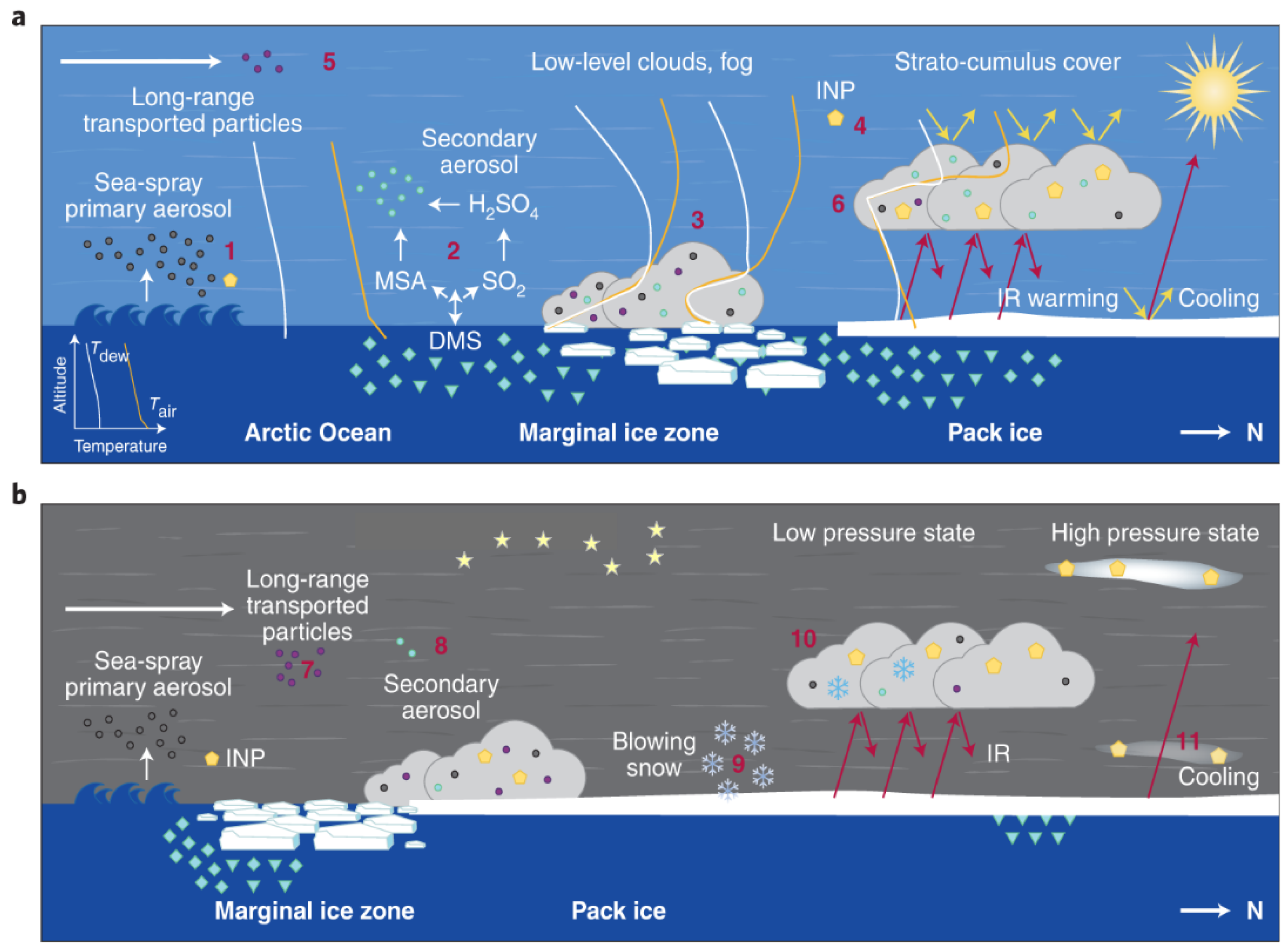
Figure 2.
Map of Ny-Ålesund on Svalbard in the European Arctic (source: Svalbardkartet; courtesy of Norwegian Polar Institute, last accessed 2024/07/26 16:32:41).
Figure 2.
Map of Ny-Ålesund on Svalbard in the European Arctic (source: Svalbardkartet; courtesy of Norwegian Polar Institute, last accessed 2024/07/26 16:32:41).
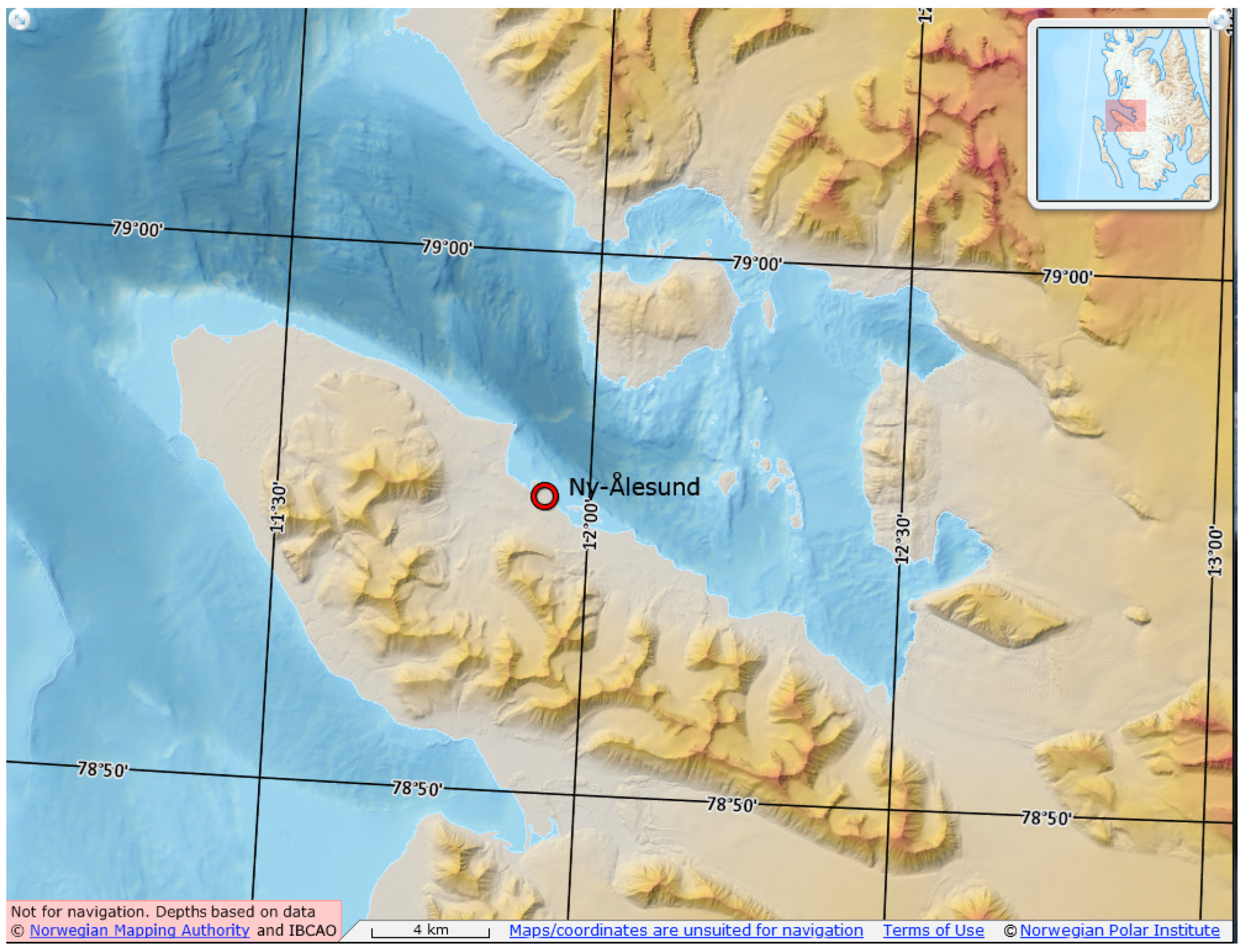
Figure 3.
Measurement time [min] for the combined data set of sun and star photometer after cloud-screening. The number of measurement points marked as clouds are also presented. For the further analysis some months will be considered without data, since the number of measurement points is too small.
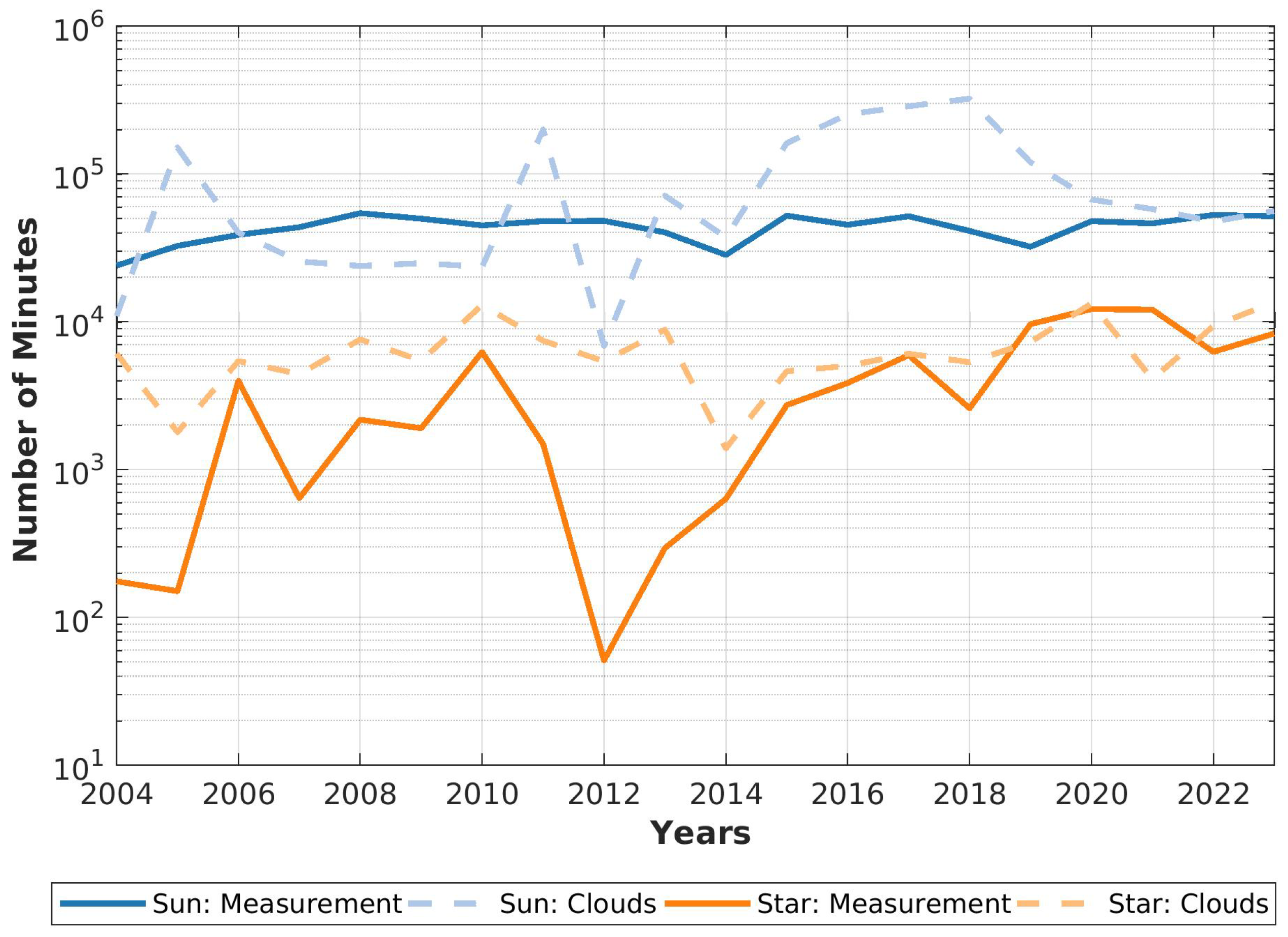
Figure 4.
Overview of combined photometer data. Every point is a daily median AOD.
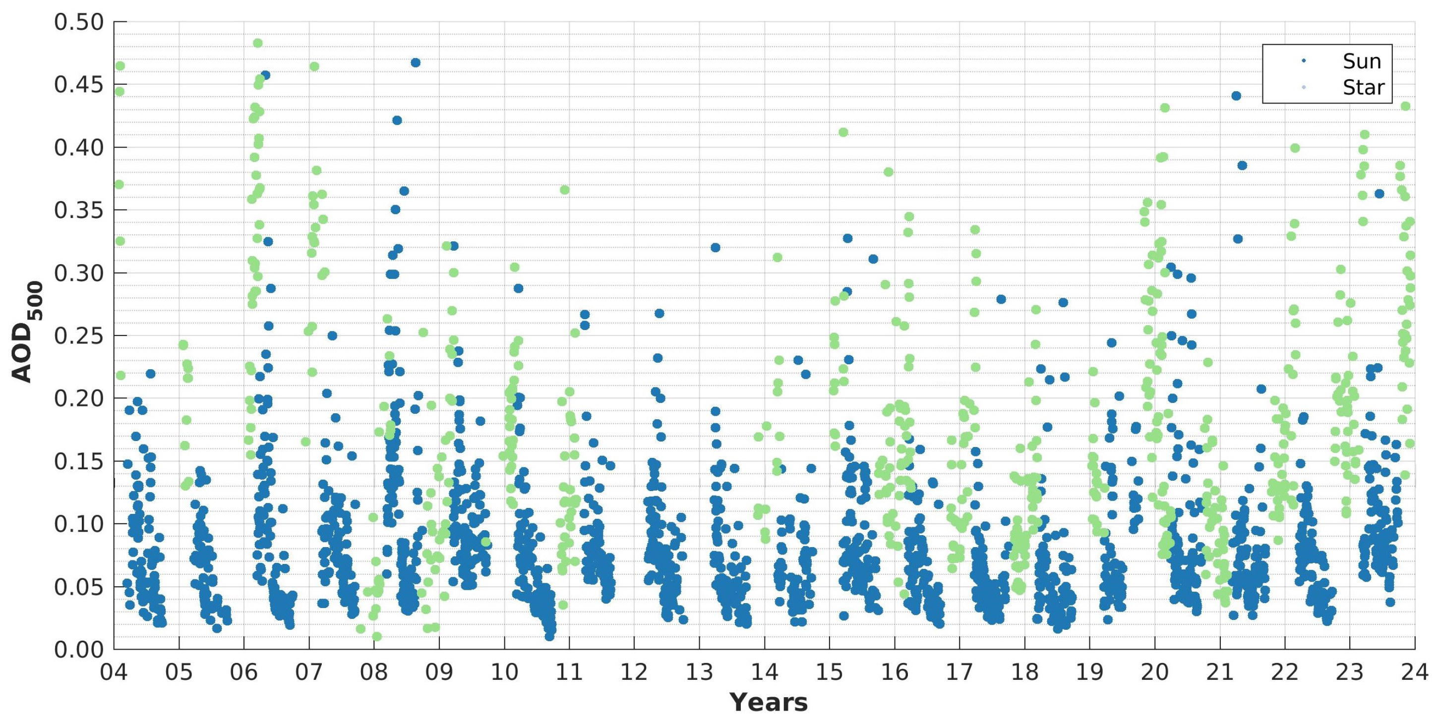
Figure 5.
The monthly median values for the AOD is shown for each year of 2004 – 2023 in grey. The blue line indicates the median of these values.
Figure 5.
The monthly median values for the AOD is shown for each year of 2004 – 2023 in grey. The blue line indicates the median of these values.
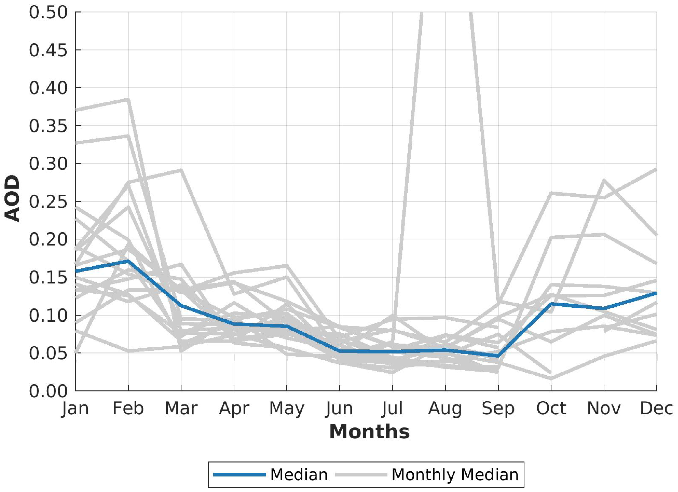
Figure 6.
Box-and-whisker plots for AOD for every month each measured by sun and star photometer. All individual data points after cloud-screening are shown. As a reference for the amount of data per month and year see Figure 3. 25th and 75th percentile are shown by the box in blue, whiskers indicated 9th and 91th percentile, median is shown by − and mean by +.
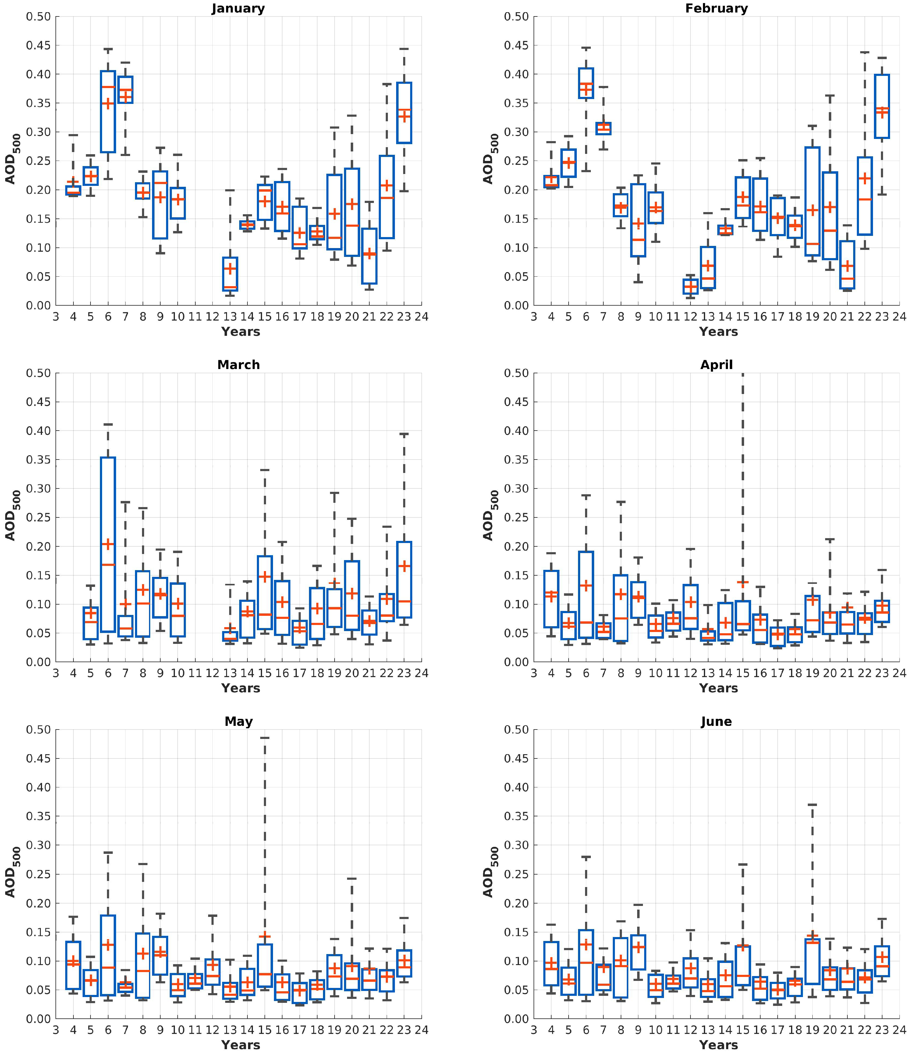
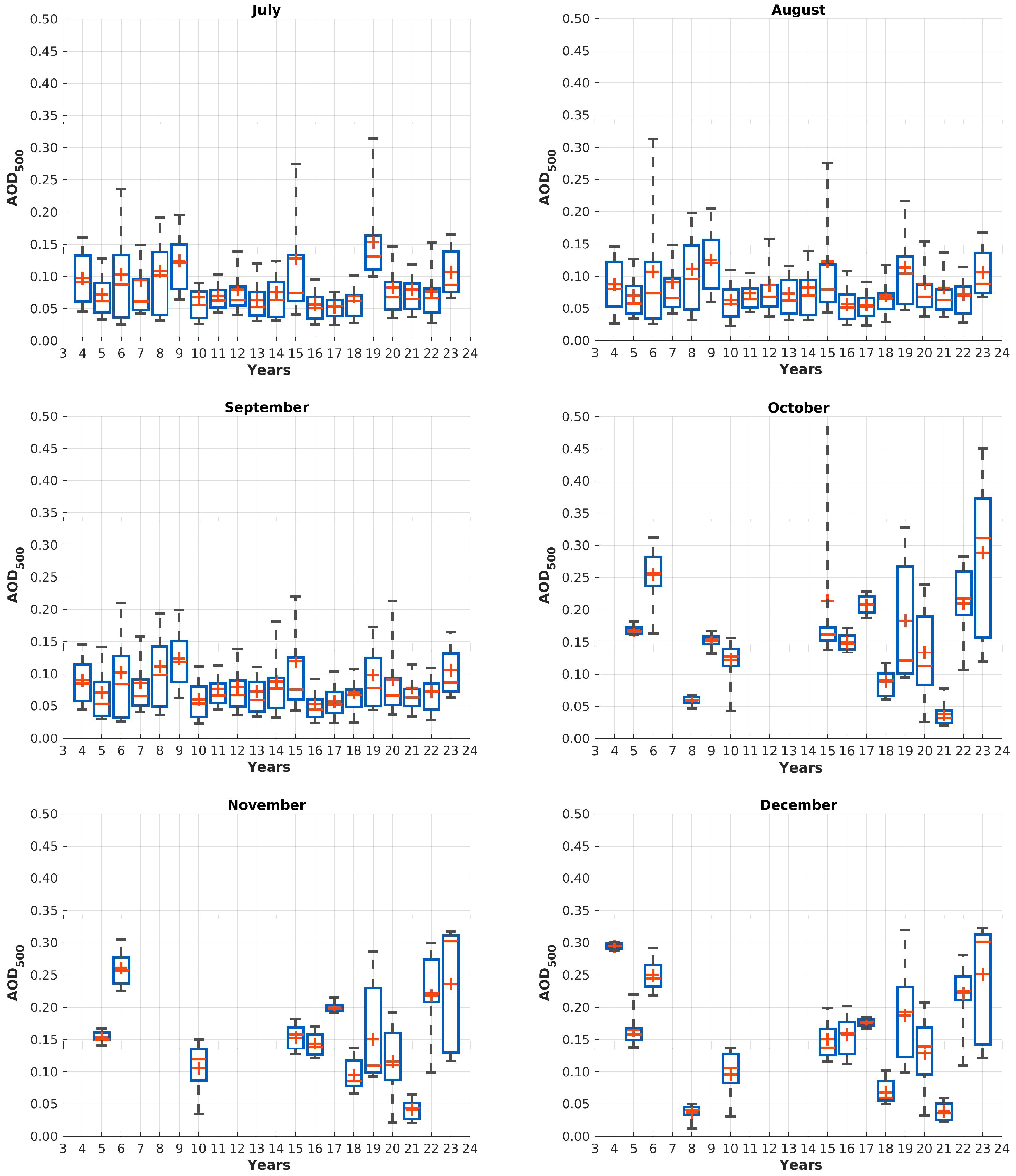
Figure 7.
Deviation from monthly AOD mean values in dependency of different years.
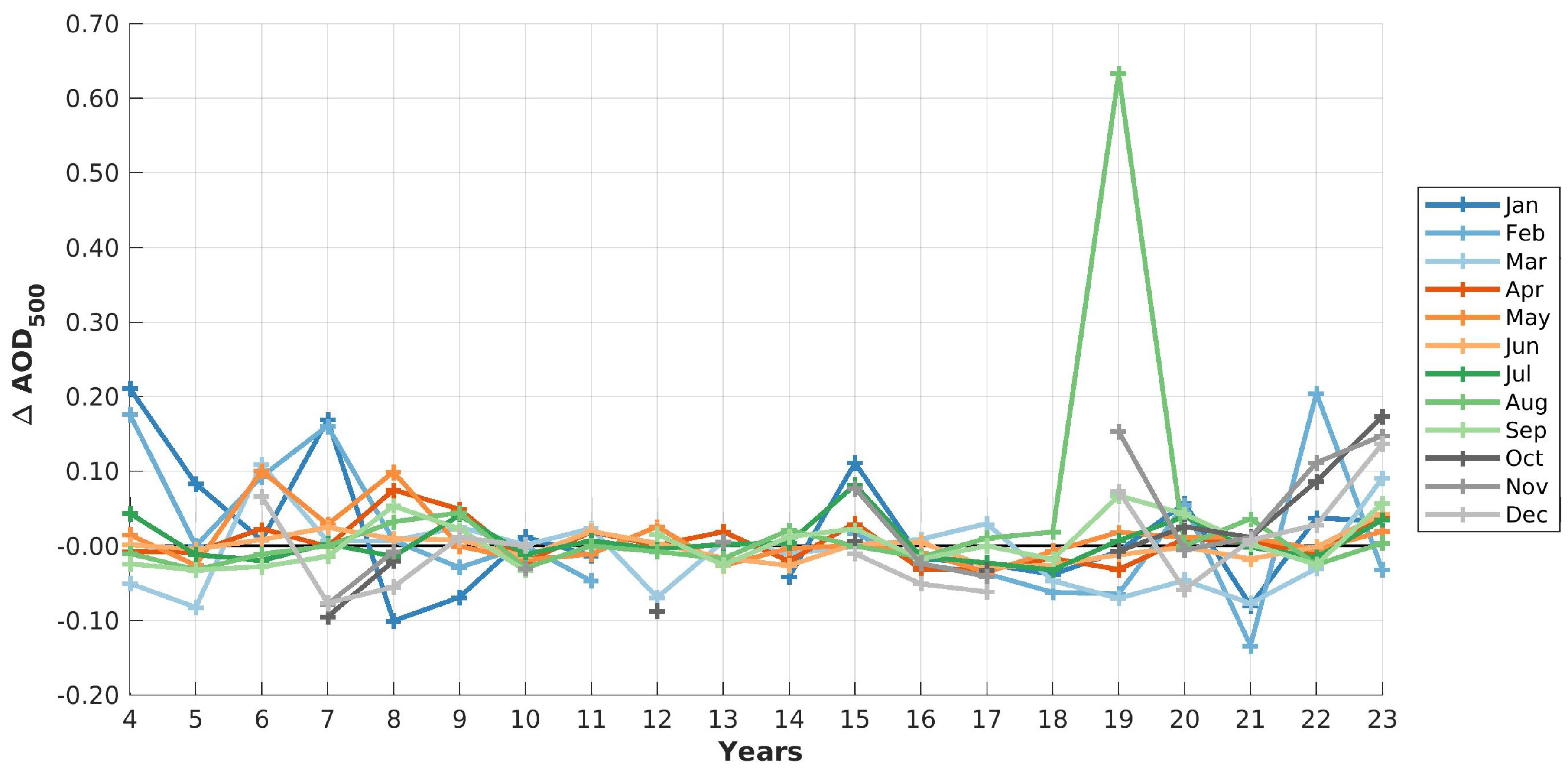
Figure 8.
Daily median of Ångström Exponent for sun and star photometer.
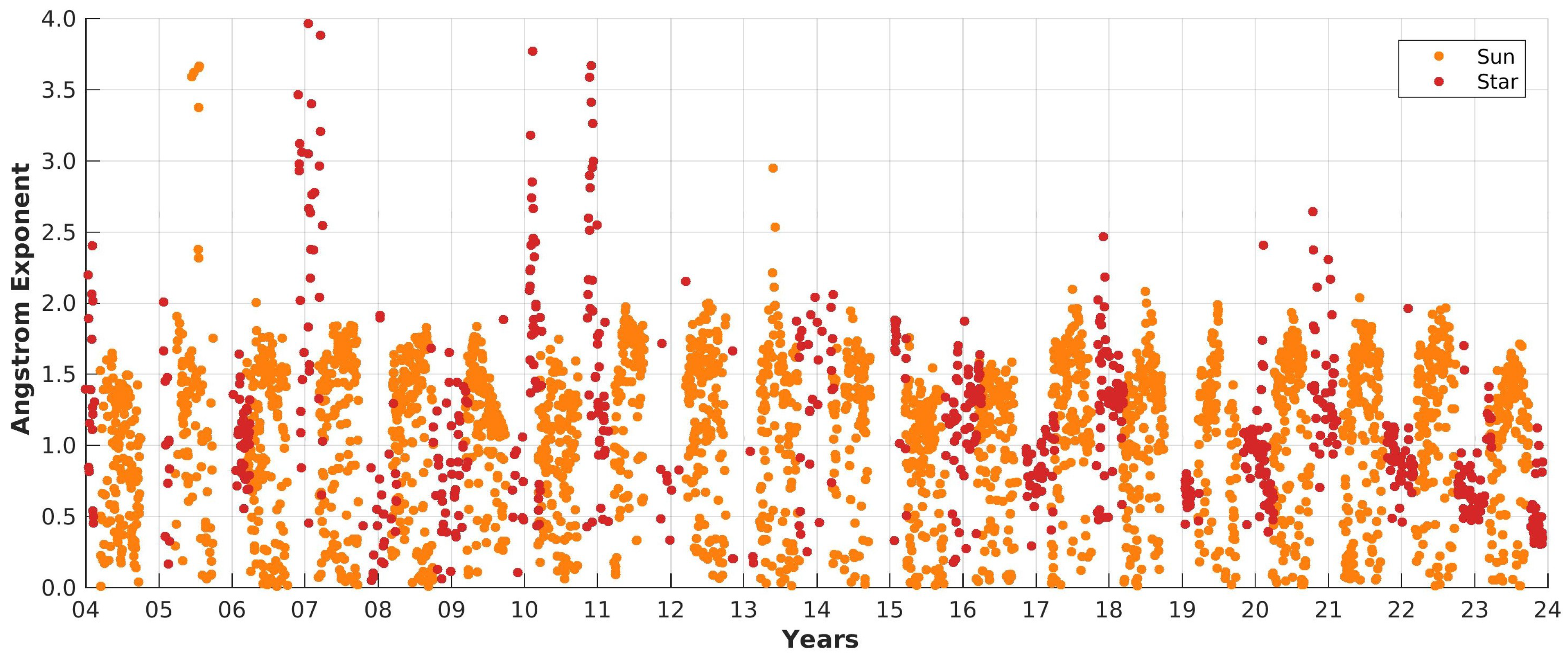
Figure 9.
Density plot of AOD and Ångström Exponent () for Sun (left) and star photometer (right) for all individual measurements from 2004 to 2023.
Figure 9.
Density plot of AOD and Ångström Exponent () for Sun (left) and star photometer (right) for all individual measurements from 2004 to 2023.
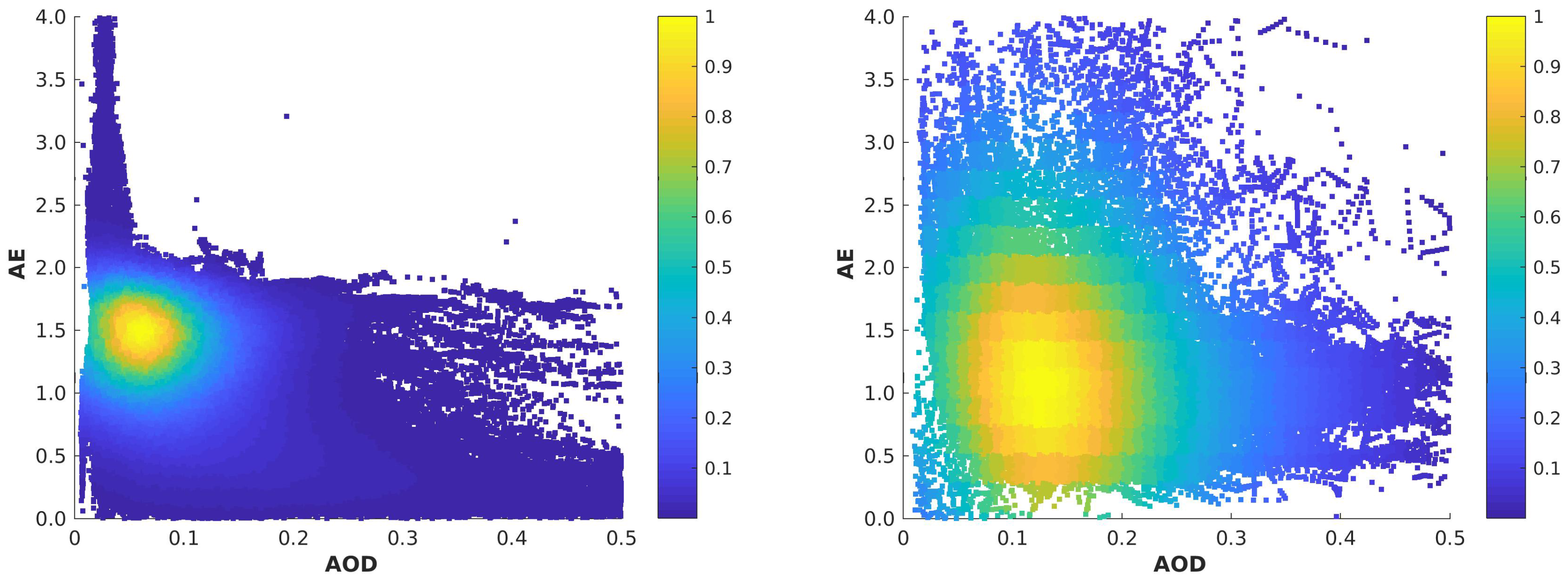
Figure 10.
Monthly median values of the Ångström Exponent is shown in grey for all of the years 2004 to 2023. The median of these annual cycle is given in orange.
Figure 10.
Monthly median values of the Ångström Exponent is shown in grey for all of the years 2004 to 2023. The median of these annual cycle is given in orange.
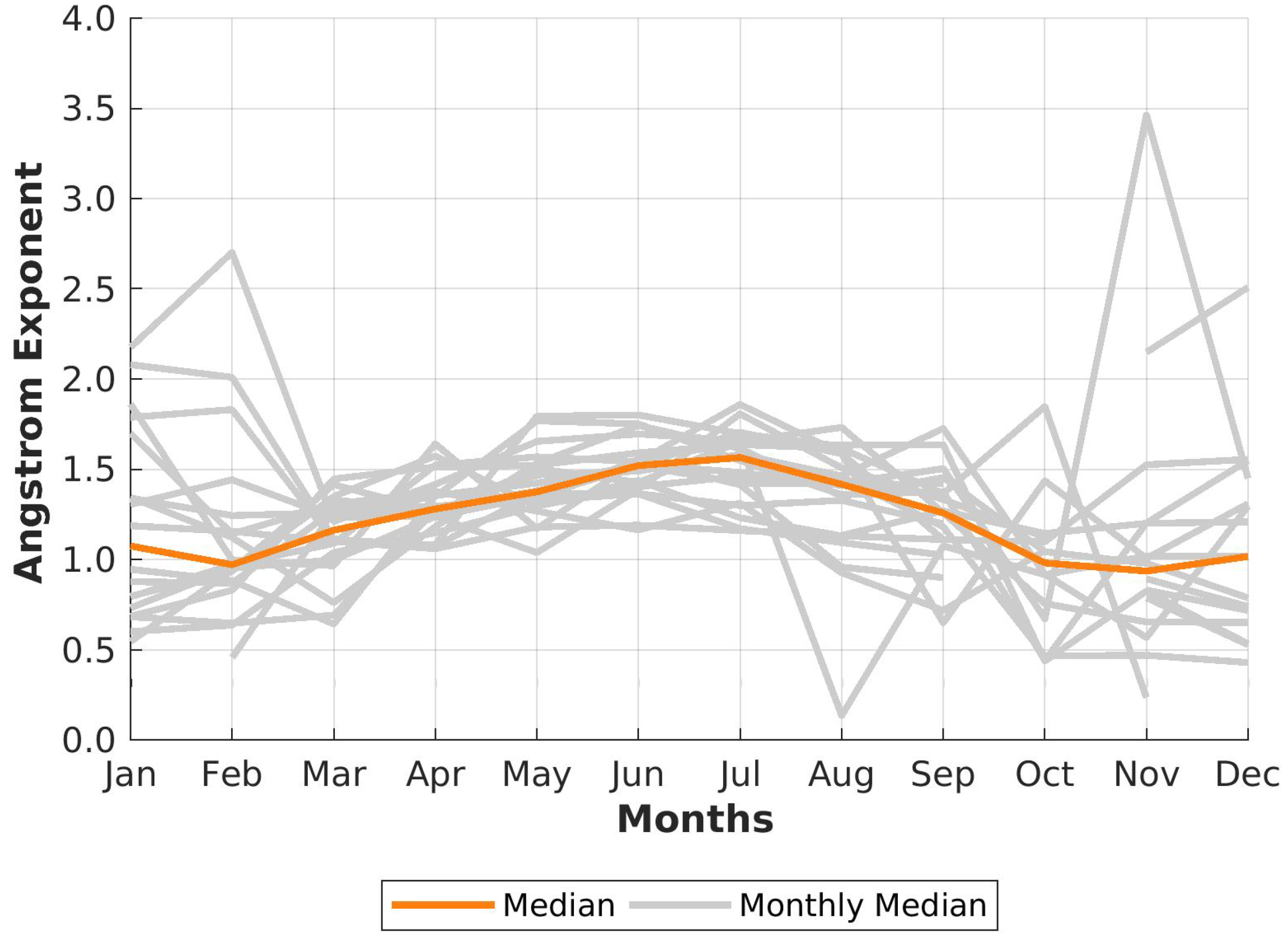
Figure 11.
Box-and-whisker plots for Ångström Exponent for every month each measured by sun and star photometer. All individual data points after cloud-screening are shown. As a reference for the amount of data per month and year see Figure 3. 25th and 75th percentile are shown by the box in blue, whiskers indicated 9th and 91th percentile, median is shown by − and mean by +.
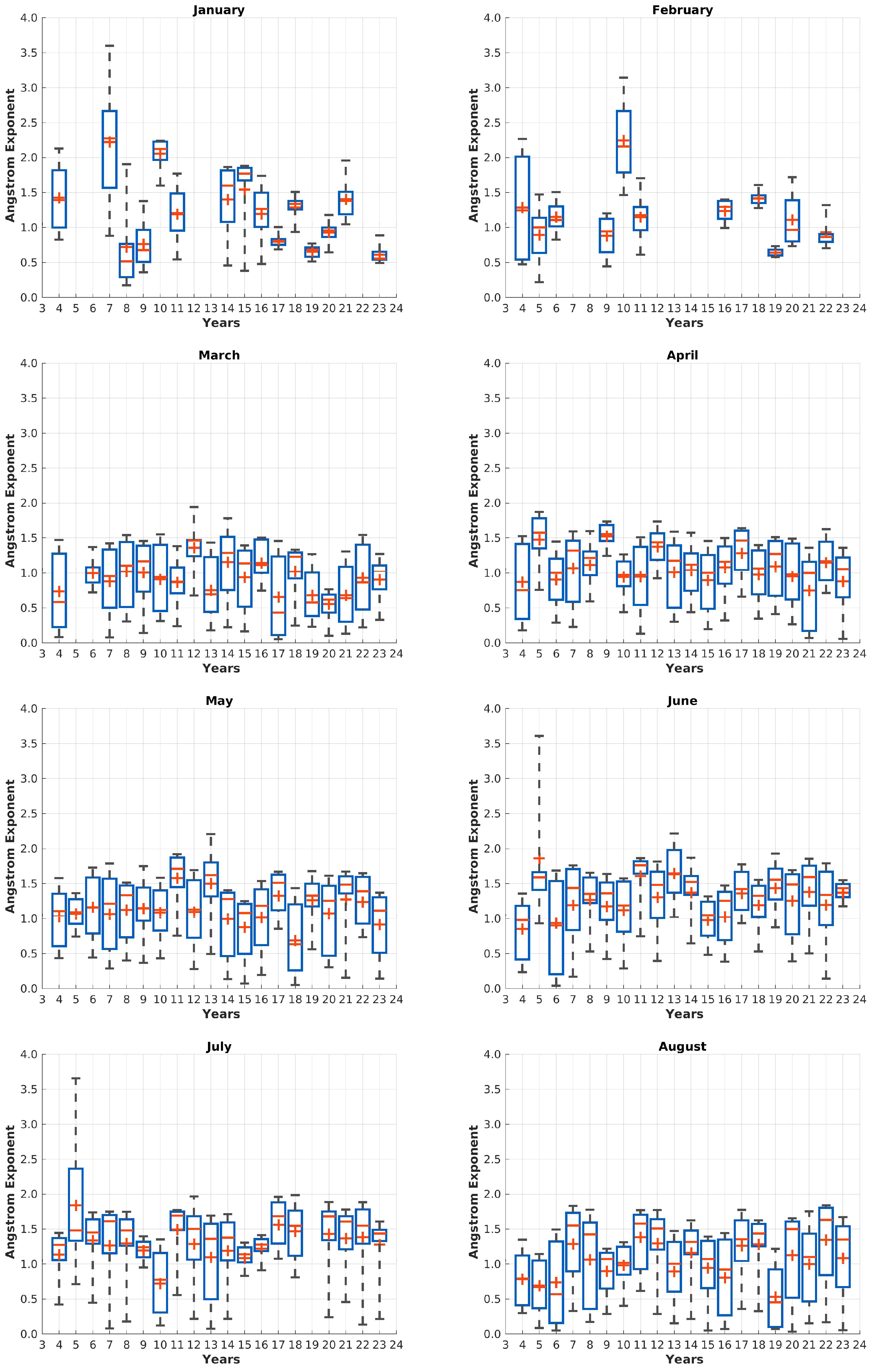
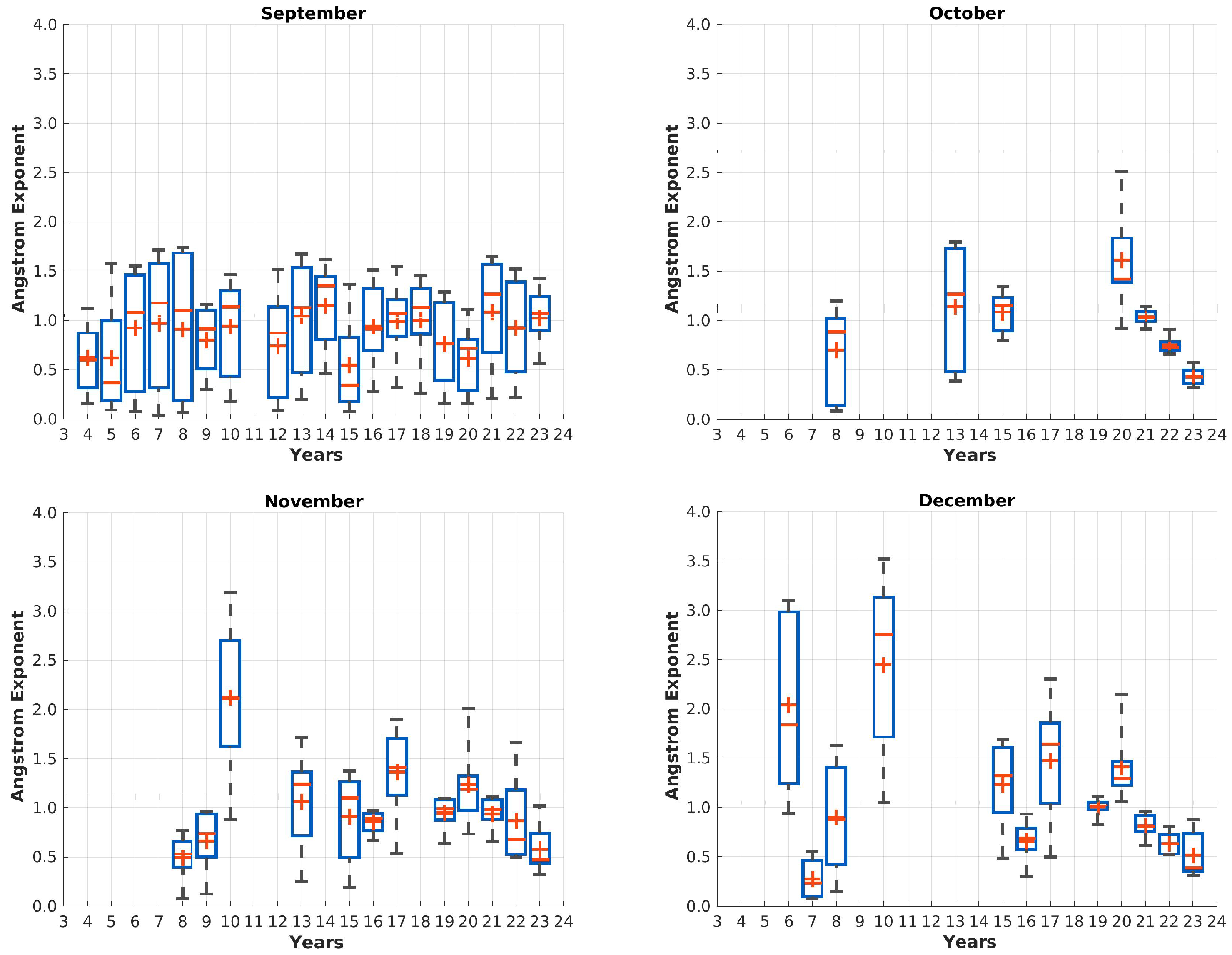
Figure 12.
Deviation from monthly mean values in dependency of different years.
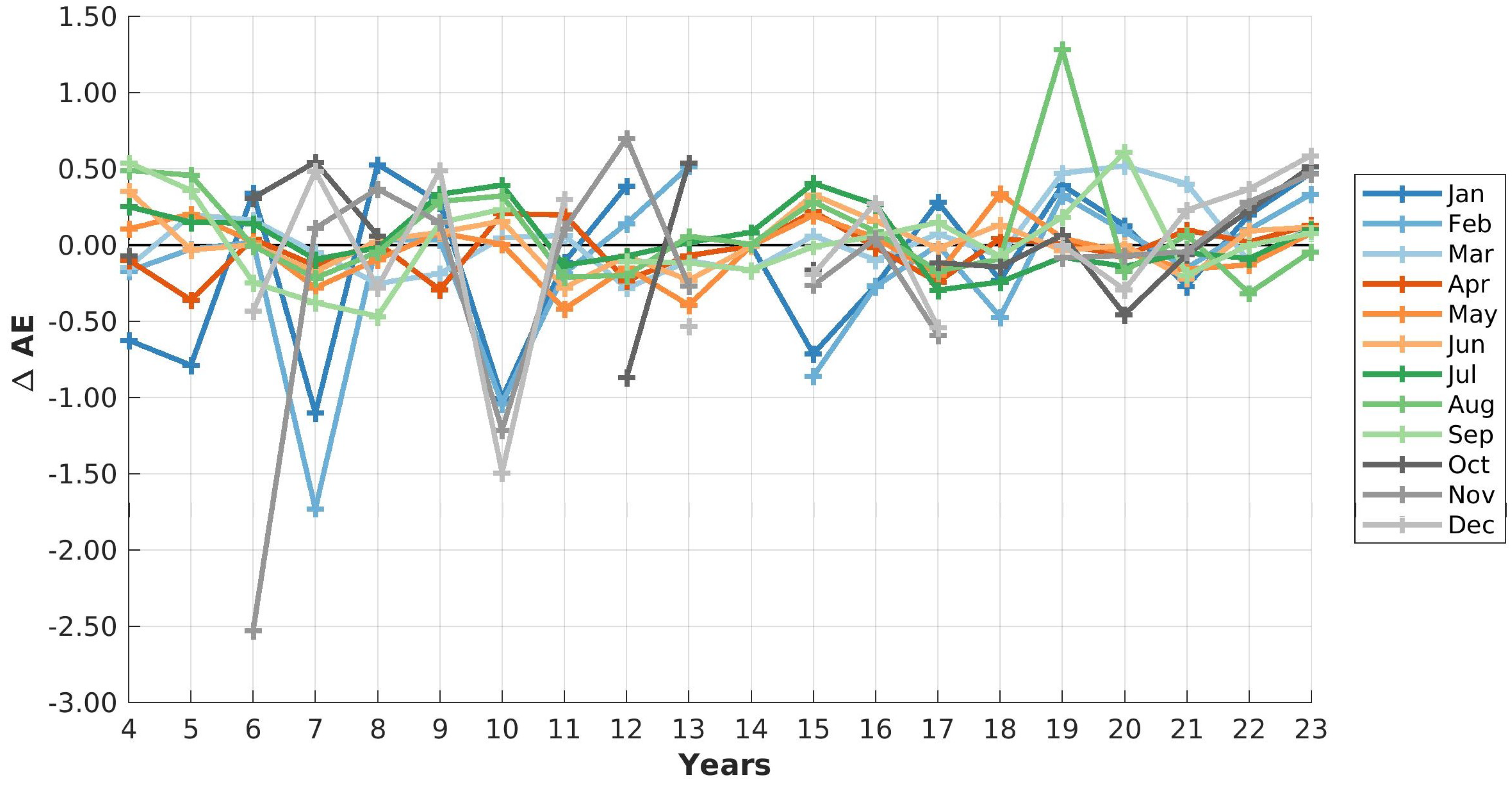
Figure 13.
One exemplary day with PSC (9 February 2020), measured by the Raman Lidar KARL in Ny-Ålesund. The PSC is clearly visible in about 20 km altitude throughout the entire day.
Figure 13.
One exemplary day with PSC (9 February 2020), measured by the Raman Lidar KARL in Ny-Ålesund. The PSC is clearly visible in about 20 km altitude throughout the entire day.
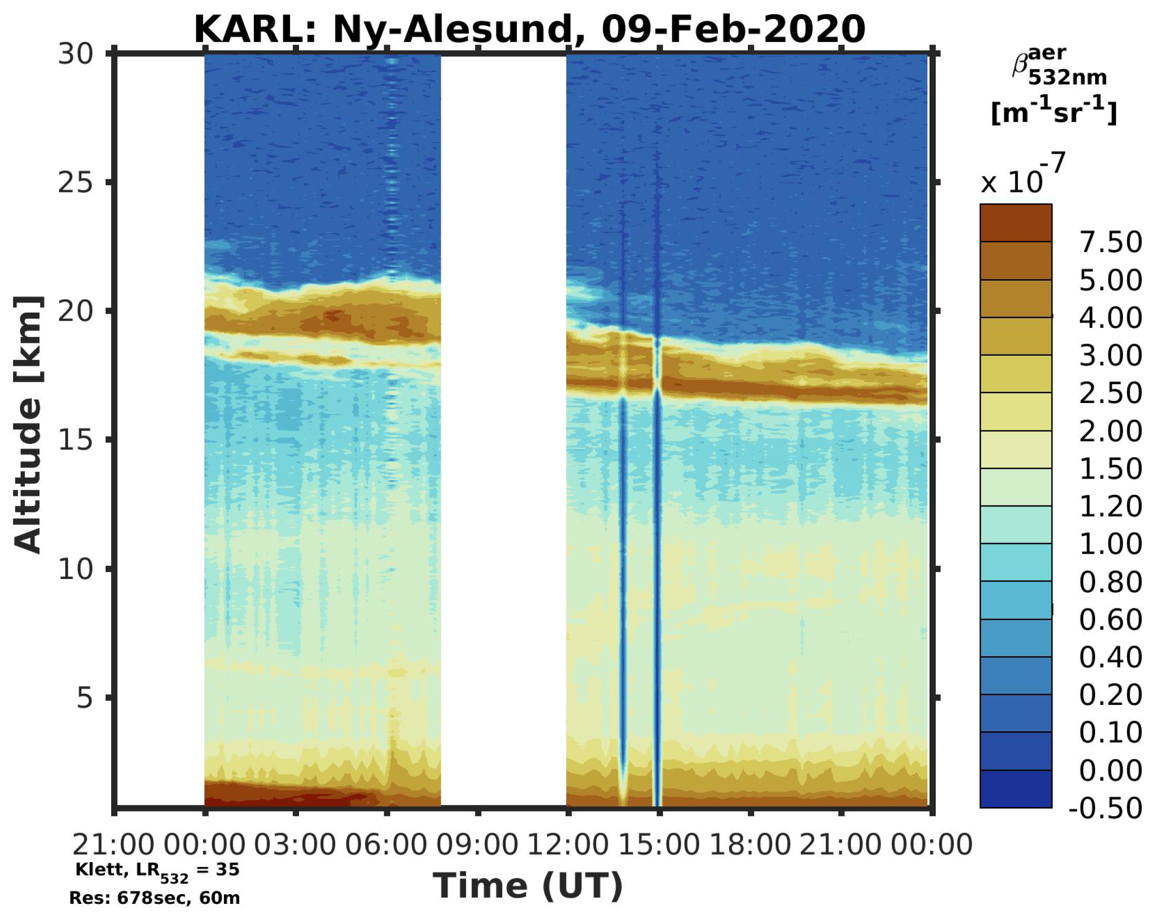
Figure 14.
Autocorrelations are shown here for every month separately for all 20 years combined (grey). The green line gives the median curve of all individual autocorrelations. The vertical lines mark the times at 1 hour and 1 day. The black diamonds indicate the inflection points.
Figure 14.
Autocorrelations are shown here for every month separately for all 20 years combined (grey). The green line gives the median curve of all individual autocorrelations. The vertical lines mark the times at 1 hour and 1 day. The black diamonds indicate the inflection points.
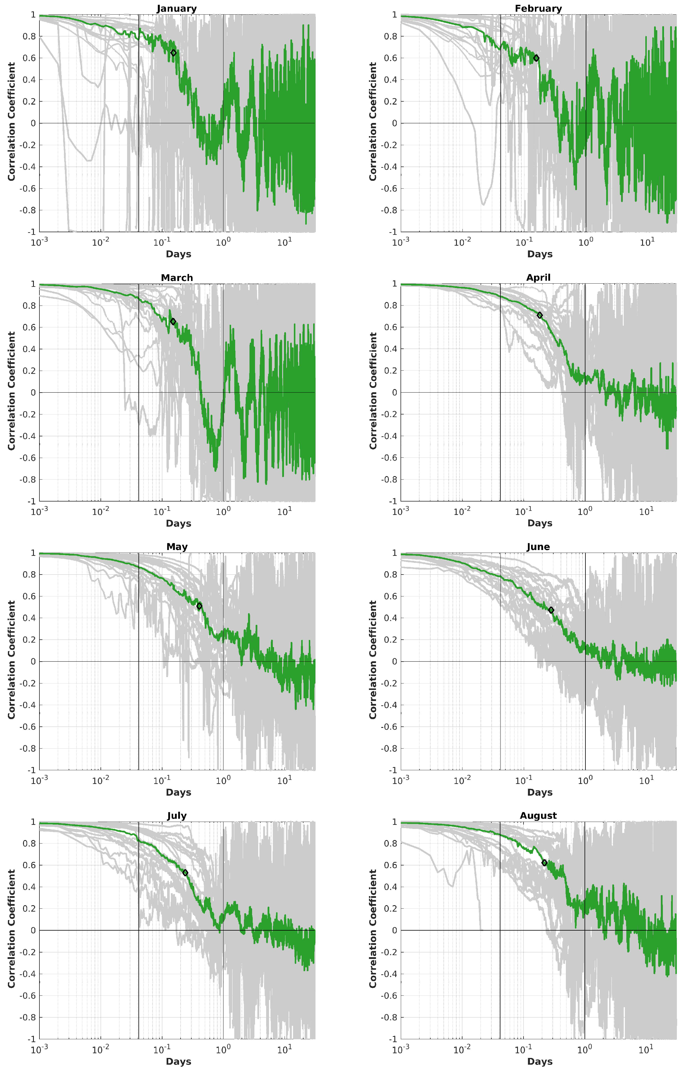
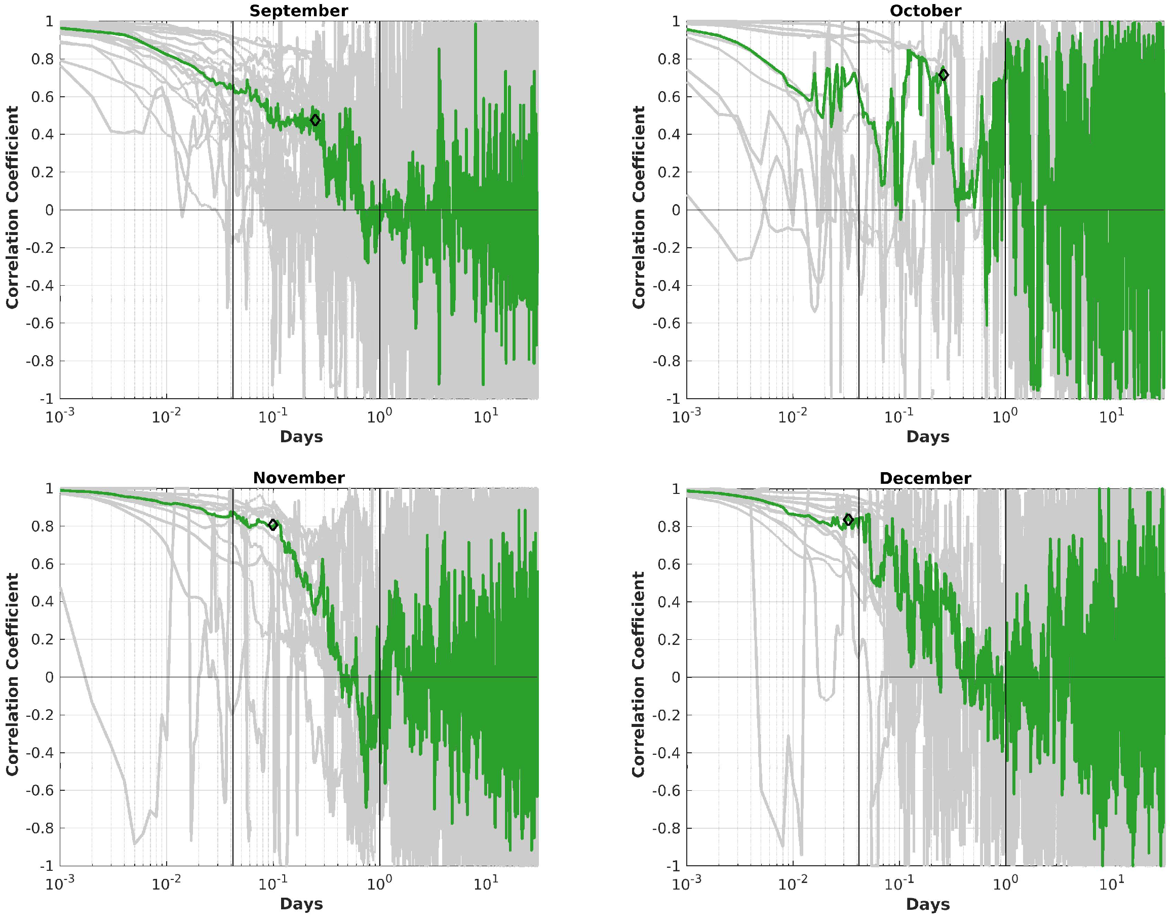
Figure 15.
Overview over the frequency spectrum for months April to August for the years 2004 – 2023 and their absolute numbers of the frequencies in the order of magnitude (blue: starting from ; red: until ). Every year is represented in five vertical bars.
Figure 15.
Overview over the frequency spectrum for months April to August for the years 2004 – 2023 and their absolute numbers of the frequencies in the order of magnitude (blue: starting from ; red: until ). Every year is represented in five vertical bars.
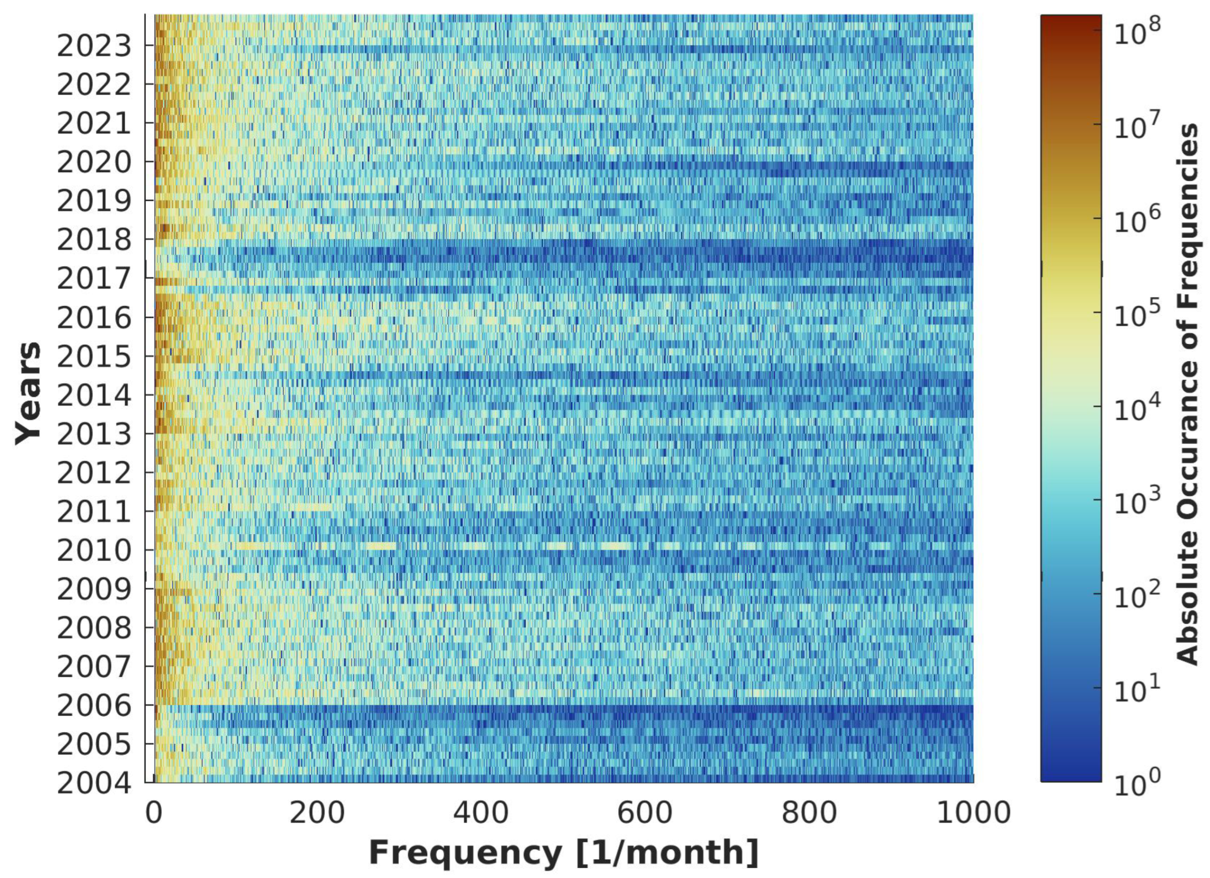
Figure 16.
Integrated frequency spectrum for different time intervals relative to the total frequency spectrum. Top: large-scale processes with a time span of several days. Mid: regional processes on a time span of several hours. Bottom: local processes on a time span of several minutes.
Figure 16.
Integrated frequency spectrum for different time intervals relative to the total frequency spectrum. Top: large-scale processes with a time span of several days. Mid: regional processes on a time span of several hours. Bottom: local processes on a time span of several minutes.
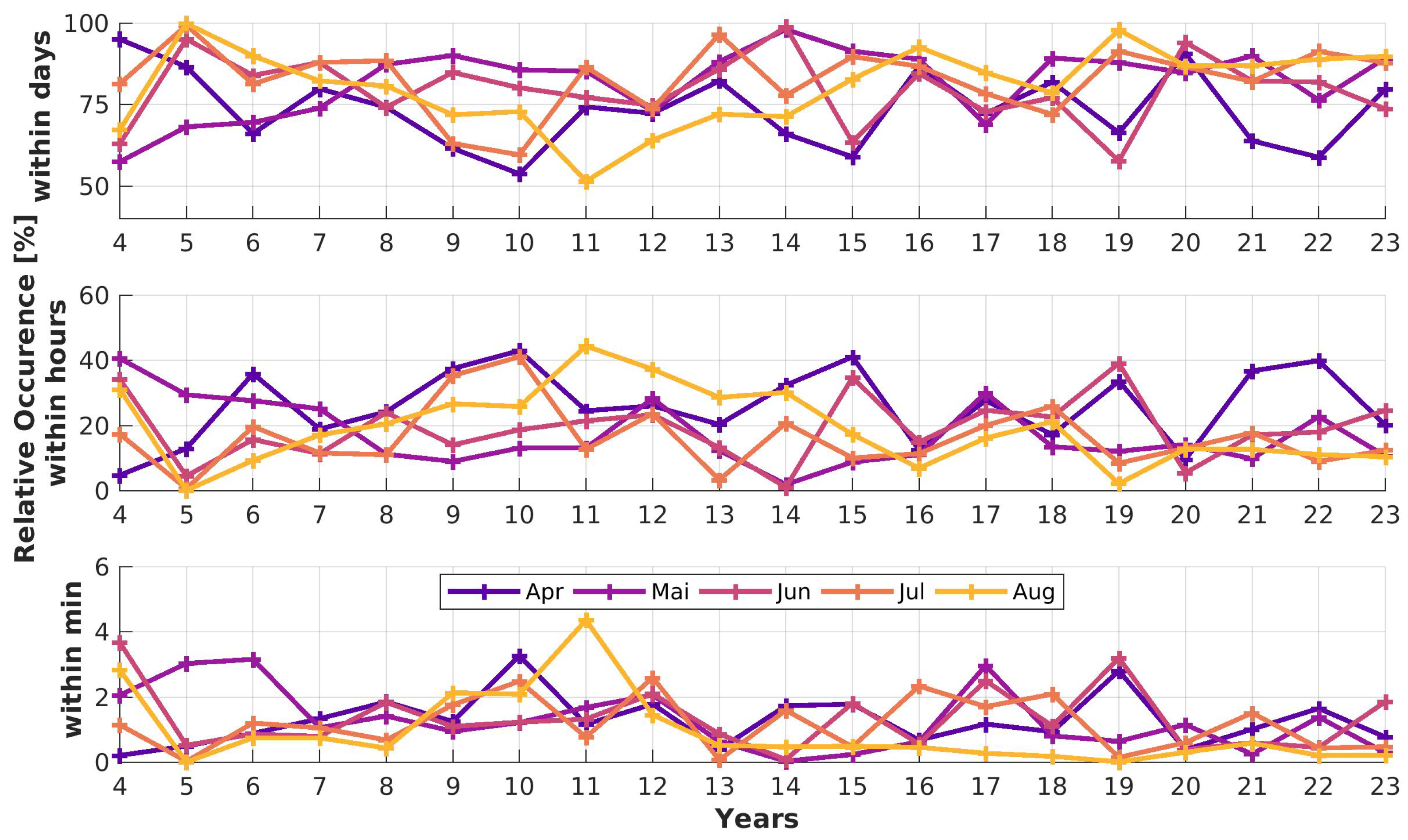
Figure 17.
Monthly median AOD values are given in blue. With a multi linear regression this AOD is reconstructed by using the above-mentioned parameters.
Figure 17.
Monthly median AOD values are given in blue. With a multi linear regression this AOD is reconstructed by using the above-mentioned parameters.
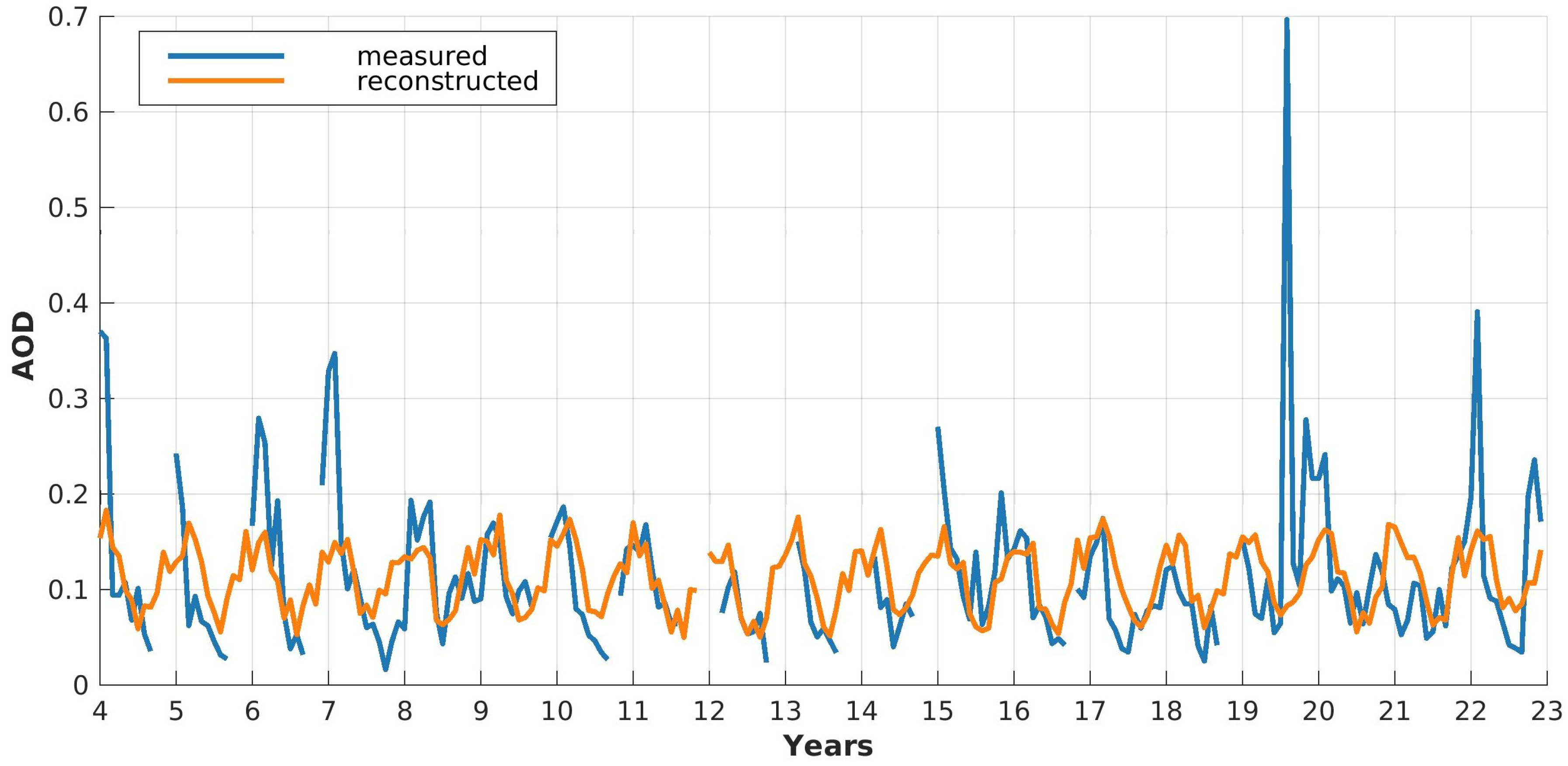
Table 1.
Relative contribution of the single terms of Equation (14) to the total error to the three exemplary wavelengths with the mean AOD of 17 December 2020 as a reference.
Table 1.
Relative contribution of the single terms of Equation (14) to the total error to the three exemplary wavelengths with the mean AOD of 17 December 2020 as a reference.
| AOD | ||||||||
|---|---|---|---|---|---|---|---|---|
| 420.0 nm | 3.0 | 75.4 | 0.1 | 20.6 | <0.1 | 0.0 | 0.0 | 0.14 |
| 500.4 nm | 2.9 | 66.3 | <0.1 | 11.2 | <0.1 | 19.4 | 0.4 | 0.11 |
| 1029.5 nm | 6.7 | 91.2 | 0.1 | 1.0 | <0.1 | 0.0 | 0.0 | 0.08 |
Table 2.
Largest error estimation for sun and star photometer in comparison for selected wavelengths. Error for sun photometer taken from Stock [21] for small airmasses.
Table 2.
Largest error estimation for sun and star photometer in comparison for selected wavelengths. Error for sun photometer taken from Stock [21] for small airmasses.
| 420.0 nm | 500.4 nm | 1029.5 nm | |
|---|---|---|---|
| Sun photometer | 0.02 | 0.01 | 0.01 |
| Star Photometer | 0.03 | 0.02 | 0.01 |
Table 3.
Deseasonalized monthly median AOD in and its standard deviation of the monthly median of for the years 2004 – 2023 with combined sun and star photometers.
Table 3.
Deseasonalized monthly median AOD in and its standard deviation of the monthly median of for the years 2004 – 2023 with combined sun and star photometers.
| Jan | Feb | Mar | Apr | May | Jun | Jul | Aug | Sep | Oct | Nov | Dec | |
|---|---|---|---|---|---|---|---|---|---|---|---|---|
| Trend | -4.30 | -4.91 | -0.82 | -0.10 | -1.67 | -0.46 | 0.12 | 5.82 | 2.15 | 10.72 | 9.30 | 3.34 |
| Std | 0.08 | 0.09 | 0.05 | 0.03 | 0.04 | 0.02 | 0.03 | 0.14 | 0.03 | 0.08 | 0.08 | 0.06 |
Table 4.
Deseasonalized monthly median and its standard deviation of the monthly median of for the years 2004 – 2023 with combined sun and star photometers. The trend is given as . Positive values indicate aerosols becoming generally smaller over time.
Table 4.
Deseasonalized monthly median and its standard deviation of the monthly median of for the years 2004 – 2023 with combined sun and star photometers. The trend is given as . Positive values indicate aerosols becoming generally smaller over time.
| Jan | Feb | Mar | Apr | May | Jun | Jul | Aug | Sep | Oct | Nov | Dec | |
|---|---|---|---|---|---|---|---|---|---|---|---|---|
| Trend | 0.55 | 0.53 | 0.17 | 0.16 | 0.04 | -0.03 | -0.23 | -0.20 | 0.01 | -0.10 | 0.91 | 0.45 |
| Std | 0.52 | 0.53 | 0.23 | 0.16 | 0.19 | 0.17 | 0.20 | 0.36 | 0.28 | 0.39 | 0.77 | 0.55 |
Table 5.
Inflection point of the median curve for every month. The corresponding duration is given in [h].
Table 5.
Inflection point of the median curve for every month. The corresponding duration is given in [h].
| Jan | Feb | Mar | Apr | May | Jun | Jul | Aug | Sep | Oct | Nov | Dec |
|---|---|---|---|---|---|---|---|---|---|---|---|
| 3.67 | 3.77 | 3.67 | 4.34 | 9.70 | 6.65 | 5.71 | 5.26 | 5.93 | 6.22 | 2.38 | 0.79 |
Disclaimer/Publisher’s Note: The statements, opinions and data contained in all publications are solely those of the individual author(s) and contributor(s) and not of MDPI and/or the editor(s). MDPI and/or the editor(s) disclaim responsibility for any injury to people or property resulting from any ideas, methods, instructions or products referred to in the content. |
© 2024 by the authors. Licensee MDPI, Basel, Switzerland. This article is an open access article distributed under the terms and conditions of the Creative Commons Attribution (CC BY) license (https://creativecommons.org/licenses/by/4.0/).
Copyright: This open access article is published under a Creative Commons CC BY 4.0 license, which permit the free download, distribution, and reuse, provided that the author and preprint are cited in any reuse.


