
Submitted:
20 July 2024
Posted:
22 July 2024
You are already at the latest version
Abstract
Leakage is important in groundwater cycle research and water resource management, the key is to construct the spatial distribution of aquitard. Influenced by natural and anthropogenic factors, the density of boreholes restricts the accuracy of aquitard structure. This paper explores the K-Nearest Neighbor (KNN) method to construct multi-layer aquitard structure in the hinterland of Songnen Plain, Northeast China, with limited boreholes, and compare it with Inverse Distance Weight (IDW) and Ordinary Kriging (OK) methods to evaluate the leakage. The KNN needs to first identify the eigenvalue-k of each layer, which is used to enhance the trainset to obtain the testset with a larger amount of sample data enhanced, and to make a prediction to obtain the 3-dimensional structure of aquitard. KNN is more accurate than the IDW and OK. The aquitrad structure obtained by the KNN is different from the IDW and OK, the thickness difference is 3.53%-54.00%, the area difference is 2.28%-23.91%, and the difference in leakage can be up to 24.51%. KNN also has a high degree of identification of aquitard edges, which can help the prevention of groundwater pollution. The results provide guidance for water balance analysis, borehole engineering design, water resources management and exploitation.
Keywords:
Leakage
; aquitard
; structure
; KNN
; trainset
; groundwater
1. Introduction
Leakage is an important recharge term for confined aquifers, and vertical water exchange between surface water, unconfined and confined groundwater is the major factors in the regional water balance. The distribution range and thickness of aquitard in the stratum is the important factor in controlling the leakage, which is also the key to controlling the quantity and quality of confined groundwater[1,2]. In the water-rich rivers and lakes around, often distributed a large number of cities and industrial and agricultural production, pressurized water mining has an important significance of water supply, aquitard can also be for the surface water and dive in the case of sudden pollution to provide security support. leakage identification is mainly by the geological boreholes to identify the spatial distribution of aquitard, and groundwater monitoring wells to monitor the level of water in different aquifers [3,4]. However, the density of boreholes and wells is limited in the zones such as rivers, lakes and wetlands [5]. In the process of interpolation, the aquitard structure obtained by common interpolation methods such as Ordinary Kriging (OK), Inverse Distance Weight (IDW) and Nearest Neighbour (NN) has bias because the hydrogeological conditions cannot be fully considered[6,7]. This is especially the case when there are few boreholes and the aquitard is not continuous. In recent years, Machine Learning (ML) such as K-nearest neighbor (KNN), Random Forest (RF) and Support Vector Machine (SVM) have been widely used for interpolation, but lack of practical application for aquitard construction and leakage analysis. The practical application of this method is lacking [8,9].
The KNN method is an upgraded version of the NN method, which is an algorithm that automatically searches for the nearest neighboring points and inverts the eigenvectors of the points to be sought through the eigenvectors of the nearest points [10,11]. The KNN method is used to improve the accuracy of interpolation in studies of stratigraphic construction [12], soil contaminant distribution [13,14], groundwater contaminant transport [15] , and ecological investigation [16,17]. The KNN method first gives the prediction samples, searches for the k samples closest to the target to be measured in the determined dataset, and finally determines the type of the prediction samples using the majority voting method, which is used to determine the type of the prediction samples, and in the practical application as the prediction purpose is varied, the dataset includes the trainset, validationset and testset. validationset and testset [18]. The core of KNN method is k-value and distance, where the distance can be physical distance or abstract distance such as similarity [19,20,21]. Most studies have pointed out that the selection of k value is the key point that affects the accuracy of KNN classification, and either too large or too small value of k will affect the accuracy of prediction [22,23]. The key issues are the way to match the actual geological conditions with the KNN method, and to provide support for leakage calculation and pollution analysis after the establishment of the aquitard structure [24,25]. The optimization of k value, the basis of grid division, and the process of data enhancement in the construction of the regional three-dimensional aquitard need to be further investigated.
Along the Nen River in the hinterland of Songnen Plain in Northeast China, the terrain is low-lying and numerous lakes and wetlands are distributed, which is not conducive to the high-density arrangement of boreholes, and there is a certain difficulty in identifying the aquitard under the wetlands around the river. In this study, a 12km×8km area in Qiqihar city area is selected to investigate the effect of KNN method on the construction of aquitard structure and leakage. The continuous stable aquifer at ~50m below the surface of the site is an important control unit for the recharge of confined groundwater, which is of great significance for water supply. On the other hand, there is a discontinuous aquitard at the ~30 m in the local area of the site, and the identification of its leakage characteristics is of great significance for the prevention, control and management of groundwater pollution. Thus, we carry out (1) to use the trainset to identify the eigenvalue-k value of each aquitard, and use the required eigenvalue-k value to enhance the data to get the testset, and get the aquitard structure by KNN method. (2) Compare the accuracy of the aquitard structures obtained by the KNN, IDW and OK methods, and further analyze the differences in the area and thickness of each layer. (3) Analyze the effect of aquitard structure on the leakage obtained by different methods, and raise the applicable background and promotion of the KNN method.
2. Materials and Methods
2.1. Site Description
The study area is located in Qiqihar City in the hinterland of the Songnen Plain in northeastern China, with high relief in the north and low relief in the south, and the main landform is the alluvial floodplain. It has a temperate continental monsoon climate with a precipitation of 415 mm, an annual mean temperature of 3.2°C, a mean temperature of -25.7°C in January, and a mean temperature of 22.8°C in July. The Nen River flows through the study area from north to south as shown in Figure 1, with small specific drop of the river, gentle current, vigorous lateral erosion and riverbed accumulation, developed river bends, wide river valleys, and numerous branching streams and river centers, islands, and wetlands are formed on both sides of the Nen River within the range of 1-2 km. The wetland has high vegetation coverage and close exchange of surface water and groundwater.
The stratigraphy of the study area is dominated by the Cenozoic, and since the Quaternary, the accumulation sediment has been deposited continuously, and the thickness of the Quaternary is 155m-159m. The lithology of the Lower Pleistocene of the Quaternary is medium sand and coarse sand, and the thickness of the strata is 17.00m-62.70m, the lithology of the Early Middle Pleistocene is thick gravelly sand, sand, and gravel, and the thickness of the stratigraphic strata is 46.75m-115.66m, the lithology of the Late Middle Pleistocene is fine-grained powdery clay, silty powdery clay, silt loam, and mud-bearing sand, with the thickness of 1.5m-21.70m. The lithology in the late Middle Pleistocene is fine-grained chalky clay, silty chalky clay, chalky soil and muddy sand, with a thickness of 1.5m-21.70m, of which the thickness of clay is generally less than 7.0m, while the lithology in the Upper Pleistocene is gravelly sand, coarse sand and other coarse-grained accumulations, with a stratigraphic thickness of 10.0m-32.30m.
The direction of groundwater flow in the study area is generally the same as that of the terrain, showing runoff from north to south. The depth of the submerged aquifer is 42.0~51.6m, and the recharge items are mainly atmospheric precipitation recharge, lateral runoff recharge and river infiltration recharge. The pressurized aquifer is distributed in 44.5~171.5m below the ground surface, and the recharge items are mainly vertical leakage recharge and lateral runoff recharge. The submerged aquifer and the pressurized water aquifer have stable aquitard, and there is a discontinuous aquitard in each of the two aquifers.
2.2. Construct the Structure of Aquitard
The aquitard in the study area consists of Shallow layer, middle layer, and deep layer, with 6 interfaces, and there are 7, 11, and 9 control points in these three layers, respectively, obtained from the borehole analysis (Figure 2). OK, IDW, and KNN methods were used to obtain the elevation of each interface and to construct a 3-dimensional aquitard structure in the study area, respectively.The KNN method is a kind of ML, and the basic idea is that, given the test samples, based on a certain distance metric, we find out the k training samples that are the closest to the data set (Eq. 1) and use the information of the k “neighbor” tables as the benchmark. The information of k “neighbor” tables is used as a baseline, and the majority voting method is used to make predictions, as in Eqs. 2 and 3[16].
In Eq.1-Eq.3, D is the data set, i.e., trainset, validationset, and testset, k is the quantity of training sample, y is the corresponding category, xi is the feature vector of the samples, LP is the distance measure, and P is an index, where weights affect closer points more than more distant points, and the larger the p-index, the greater the influence of closer points.
2.3. Eigenvalue-k Identification
The data in the training set of each layer is limited and the location of each training data presents irregularity, so it is not suitable to mechanically define the same k for each layer when applying the KNN method [13,25]. Take the average distance between sample points as the interval, the study area was divided into 10×7 total 70 grids, the size of each grid is approximately 1km2, and the center of the grid without original boreholes was used as virtual boreholes. The KNN method was utilized to form a trainset from the initial 13 original boreholes for training. Shallow Layer, Middle Layer and Deep Layer on a total of 6 interfaces, the same layer of upper and lower interfaces selected the same eigenvalue k value, in k < 5 can not get the prediction results, so choose 5 as the initial eigenvalue-k value. Assigning k=5, 6 and 7 to predict the elevation of the virtual borehole respectively. The original boreholes were merged with the virtual boreholes to form validationset, and the computed elevations of B1-S, B7-S, B8-S, B3-M, B6-M, B7-M, B14-M, B3-D, B6-D, and B13-D were predicted for the centrally located identified point locations, and the accuracy of the eigenvalue-k is obtained for each eigenvalue by comparing them with the actual elevations.
2.3. Data Enhancement
Enhance the training set based on eigenvalue-k. The virtual sample points are selected to form a validation set with the data in the original training set [26]. Among the KNN prediction results obtained from each eigenvalue-k layer, the virtual grid points with validation accuracy greater than 60% are used as data enhancement points[27], which together with the original 13 boreholes form the Testset, and the Testset is used for the aquitard construction.
2.4. Leakage Analysis
There is a close relationship between the groundwater leakage and the structure of the aquitard, according to Equation. 4, the area of the aquitard is positively correlated with the leakage and negatively correlated with the thickness of the aquitard. The two parameters of area and thickness are very important to calculate the leakage.
In Eq.4, Q represent the quantity of leakage, Kv represent the vertical hydraulic conductivity, ΔH represent the head difference of the two aquifer, and A and M is the area and thickness of aquitard, respectively.
In the context of aquitard lithology and its permeability to determine, the ΔH and Kv remain constant, the area and thickness ratio of A/M could determines the quantity of leakage. Gridding the study area, the A∙ΣM of the aquitard can indicate the quantity of leakage, and the comparison of the A∙ΣM obtained by the three methods of KNN, OK, and IDW is used to determine the influence of the morphology of the aquitard structure layer obtained by different methods on the leakage.
3. Results
3.1. Eigenvalue-k Values of KNN
The selection of eigenvalue-k has a significant effect on the prediction accuracy as shown in Figure 3. In Shallow layer, boreholes are mainly distributed in the northeast part of the study area, and the average value of accuracy is 76.07% when eigenvalue-k=5, which is higher than that when eigenvalue-k = 6 and 7 (accuracy 70.81% and 62.94%, respectively), and the selection of eigenvalue-k in this layer is 5. In Middle Layer. boreholes are distributed evenly in the study area and the average accuracy is 74.55% when eigenvalue-k=7, which is higher than when eigenvalue-k = 5 and 6 (accuracy 68.55% and 68.56%, respectively), and the selection of eigenvalue-k for this layer is 7. In Deep Layer, the boreholes are distributed west-centrally in the study area, and the accuracy is higher than the selection of eigenvalue-k for this layer when eigenvalue-k=6, the average accuracy is 61.44%, which is higher than that of eigenvalue-k = 5 and 7 (accuracy 55.29% and 52.83%, respectively), and the eigenvalue-k of this layer is chosen as 7. The eigenvalues obtained from the three layers are 5, 7, and 6, respectively.
3.2. Enhance of the Trainset
The control points within the study area are limited and distributed far apart, and the number of borehole data in the respective trainset of the three layers does not correlate with the resulting eigenvalue-k, however, neither does it correlate with the accuracy of the predictions. This is consistent with the findings of others in related studies [12,25,28]. In the case of eigenvalue-k choosing too small will result in the prediction not being able to be made, and choosing too large will cause the prediction to be disturbed by distant control points, creating a large deviation [16,29]. Based on this, with up to 8 grid centers around the adjacent perimeter of each grid point, the data Enhance Area is set as shown in Figure 4, and among the KNN prediction results obtained from each layer of eigenvalue-k, the virtual grid points with an accuracy of more than 60% are selected as the data enhancement points, and the data enhancement points are set as S14-S18 in the Shallow layer, Middle layer, and Deep layer, respectively. in Shallow layer, Middle layer and Deep layer are S14-S18, M14-M24, and D14-D22, respectively.These enhancement points together with the original boreholes form the Testset with 10, 22 and 18 data in the three layers, respectively.
3.3. Aquitard Structure
The stratigraphic structure of the study area is relatively simple, and the distribution trend of the layers obtained from the KNN, IDW, and OK methods is basically the same, as shown in Figs. 5a and b. The Shallow Layer is distributed in the northeastern part of the study area, and it is gradually annihilated in the central part of the study area, the Middle Layer is distributed continuously in the whole area, and the Deep Layer is missing in the northeastern part of the study area. The thickness and area of the aquitard obtained by KNN, IDW, and OK methods are significantly different. In the Shallow layer, the average thicknesses of the KNN, IDW, and OK methods are 3.11m, 2.96m, and 1.43m, respectively (Figure 5c), and the areas are 46.2km2, 49.3km2, and 56.9km2, respectively (Figure 5f). The differences in thicknesses between the KNN method and the IDW and OK methods are 5.01% and 54.00%, and the differences in areas are 5.01% and 54.00%, respectively. 54.00%, and the area difference is -6.52% and -23.91%, respectively. In Middle layer, the average thicknesses obtained by KNN, IDW and OK methods were 3.17m, 3.78m and 2.71m, respectively (Figure 5d), and the differences between the thicknesses obtained by KNN method and those obtained by IDW and OK methods were -6.68% and 14.33%, respectively. In Deep layer, the average thicknesses obtained by KNN, IDW and OK methods are 2.82m, 2.61m, and 1.95m (Figure 5e), and the areas are 179.5km2, 175.4km2, and 198.2km2 (Figure 5g), and the differences of thicknesses obtained by the KNN method with those obtained by IDW and OK are -3.53% and 22.67%, and the differences of areas are -6.68% and 14.33%, respectively. 22.67%, and the area difference is 2.22% and -10.61%, respectively. Overall, the three methods constructed aquitard structures, and the Shallow Layer with few points and discontinuous distribution had the most significant differences.
4. Discussion
4.1. Accuracy of Aquitard Structure
The B1-S, B7-S, B8-S, B3-M, B6-M, B7-M, B14-M, B3-D, B6-D, and B13-D prediction point data were removed from the trainset, a new validationset was set up, and the elevations of the above predicted points were predicted using the KNN, IDW, and OK methods, respectively, and the accuracy was assessed based on Mean Absolute Error (MAE), Mean Square Error (MSE) error evaluation metrics to assess the accuracy. As shown in Table 1, in Shallow layer, Middle layer and Deep layer, the MAE and MSE of KNN method are lower than those of IDW and OK method. However, algorithms such as IDW and OK need to make certain conditional assumptions on the data before interpolation , which are assumptions of mathematical significance [30,31], and the KNN method is a kind of machine learning method, and the model structure built during the data training is based on the actual data [16,28],. The model structure established in the process is based on the actual geological conditions, with reference to the deposition characteristics of the sediments, and the eigenvalue-k of the vertical layers and different horizontal partitions are obtained through the machine learning process, which predicts the data within a certain effective range, and avoids the influence of the conditional assumptions on the predicted data effectively.
The construction of the geologic structure of the aquitard layer is related to the distribution density and the number of boreholes. In Shallow layer with a small number of samples, the spatial heterogeneity of the aquitard structure is larger due to the inability to further expand the density of boreholes due to natural geographic and anthropogenic factors[31,32]. The the MAE of the KNN method is reduced by 23.5% and 27.7% compared with the IDW and OK methods, respectively, and the reduction is higher than that of the Middle layer (17.2% and 15.9%, respectively) and Deep layer (12.1% and 16.4%, respectively), the results show that in the small-sample calculation of limited borehole data, the KNN method based on machine learning has more prominent advantages than OK and IDW methods, and it is more practical for the construction of aquitard layers using the KNN method.
4.2. Effect of Aquitard Structure on Leakage
Since the thickness and area of the aquitard layers obtained by the KNN, IDW and OK methods are different, as shown in Figure 6, there are obvious differences in the A∙ΣM obtained by the three methods, and in this study, assuming that the water level in the aquifer above and below the aquitard layer is constant, and the permeability coefficient of the aquitard is constant in the vertical direction, the A∙ΣM obtained by IDW is higher than that of KNN method in each layer, and that of OK is lower than that of KNN method. The A∙ΣM obtained by KNN method is higher than that by IDW method and lower than that by OK method in all layers, which shows the significant effect of the methods on the heterogeneity of the layer of aquitard. The deviation of the A∙ΣM obtained by KNN method from the IDW and OK methods in the Shallow layer is 16.17% and 24.51%, respectively. In Middle layer, the A∙ΣM deviation is 6.67% and 14.32%, and in Deep layer, the A∙ΣM deviation is 1.13% and 3.44%, respectively. It can be seen that the A∙ΣM deviations of the KNN method from the IDW and OK methods in both Shallow layer and Middle layer are significantly larger than those in Deep layer, up to 24.51%, which cannot be ignored in general leakage calculations as other research mentioned [2,6].
In the Middle Layer, the main factor affecting the leakage is the thickness, while in the Shallow Layer, the factors affecting the leakage are both thickness and area. In the study area, Middle Layer is an important channel for vertical recharge of diving and pressurized water, and the difference of the calculated leakage will have an impact on the assessment of the water balance of pressurized water.However, the Shallow Layer is distributed in the range of ~30 m below the ground surface, and the upper aquifers are fine sand and medium sand with good permeability, which has a poor blocking ability to pollutant components, and the Shallow Layer is composed of clay and chalky clay, which can block the shallow surface of the ground. The Shallow Layer is composed of clay and silty clay, which can prevent the downward migration of pollutant components in the shallow part of the surface, and the fine delineation of the distribution range of this layer using the KNN method can provide support for the pollutant migration investigation and research, and serve the planning and policy management of industry and agriculture.
4.3. Advantage of KNN Method
In this study area, the geomorphologic features of the Nen River and its shore, which traverse the central part of the study area, restrict the placement of boreholes, leading to the problem of annihilation edge blurring in the Shallow layer and uncertainty in the thicknesses of the Middle Layer and Deep Layer. The use of KNN method provides an alternative means to solve the above problems. The research on KNN can be further extended to the research related to the aquitard, such as the bottom sediment layer of rivers and lakes, and the thickness of the surface layer of wetlands, all of which have the characteristics of few control points, unclear continuity, and the leakage or infiltration volume is extremely important to the regional water circulation [16,33,34]. Moreover, the process of constructing the structure of the aquitard based on the KNN method is suitable for optimizing the placement of the drill holes. On the one hand, based on the accuracy of the KNN method prediction in the constructed grid, additional boreholes need to be placed in grids with low accuracy. On the other hand in areas where boreholes cannot be placed in a larger area, the machine learning method within KNN guides the design of the well cluster program at the edge of the area. In summary, the KNN method effectively improves the accuracy of people’s investigation and understanding of the aquitard and leakage, and can be extended to similar applications of the aquitard at the bottom of the surface water body, which contributes to the theoretical study of hydrogeology, and has the value of use in targeting the layout scheme of the well clusters and the monitoring sites to guide the production practice.
5. Conclusions
In this paper, we constructed the structure of multilayered aquitards in the hinterland of Songnen Plain, Northeast China, by K-Nearest Neighbor (KNN), and compared it with the aquitard structure constructed by Inverse Distance Weight (IDW) and Ordinary Kriging(OK) methods, to evaluate the effect of the different construction methods on the leakage. The main conclusions are as follows (1) The key of the KNN method is to recognize the eigenvalue-k of the aquitard in different layers to reduce the effect of uneven distribution of boreholes, and the eigenvalue-k is too small to be operational, and too large to be easily interfered by the distant control points. (2) The structure construction of KNN method for the discontinuous aquitard with few control points is in line with the actual geological conditions, the thickness and area of the aquitard obtained by KNN and IDW and OK methods have differences, the thickness difference is 3.53%-54.00%, and the area difference in the discontinuous aquitard is 2.28%-23.91%. (3) The structure of aquitrad structure constructed by different methods directly affects the quantity of leakage up to 24.51%, and the identification of the edge of the aquitard is higher, which is helpful for the prevention, control and management of groundwater pollution. It’s valuable for analyzing the regional water balance and providing guidance for water resources management and development and utilization.
Author Contributions
Conceptualization, Z.D.. and Y.L; methodology, Y.C.; software, Y.D.; validation, Y.D., Y.Z. and Y.C.; formal analysis, X.X.; investigation, Y.Z.; resources, Z.D.; data curation, Y.D..; writing—original draft preparation, Z.D.; writing—review and editing, Y.C.; visualization, Y.Z.; supervision, Y.Z.; project administration, Z.D.; funding acquisition, Y.Z.
Funding
Please add: This research was supported by the National Natural Science Foundation of China (Nos. 42077170 and U19A20107).
Data Availability Statement
Not applicable.
Acknowledgments
The authors would like to thank the editors and reviewers of Water for their thoughtful and constructive comments, which helped improve this paper substantially.
Conflicts of Interest
The authors declare no conflicts of interest.
References
- Pulla, S.T.; Yasarer, H.; Yarbrough, L.D. GRACE Downscaler: A Framework to Develop and Evaluate Downscaling Models for GRACE. Remote Sens 2023, 15(9), 2247. [Google Scholar] [CrossRef]
- Wang, J.; Ma, Z.; Zeng, J.; Chen, Z.; Li, G. Numerical Study on the Influence of Aquitard Layer Distribution and Permeability Parameters on Foundation Pit Dewatering. Water 2023, 15(21), 3722. [Google Scholar] [CrossRef]
- Edwards, J.; Lallier, F.; Caumon, G.; Carpentier, C. Uncertainty management in stratigraphic well correlation and stratigraphic architectures: A training-based method. Comput Geosci 2018, 111, 1–17. [Google Scholar] [CrossRef]
- Lv, S.; Zhu, Y.; Cheng, L.; Zhang, J.; Shen, W.; Li, X. Evaluation of the prediction effectiveness for geochemical mapping using machine learning methods: A case study from northern Guangdong Province in China. Sci Total Environ 2024, 927, 172223. [Google Scholar] [CrossRef] [PubMed]
- He, L.; Liu, J.; Lei, S. : Chen, L. A hybrid coupling model of groundwater level simulation considering hydrogeological parameter: a case study of Nantong City in Eastern China. Water Supply, 2023, 23(10), 4286-4302.
- Zuo, C. , Pan, Z., Yin, Z, Guo, C. A nearest neighbor multiplepoint statistics method for fast geological modeling. Comput Geosci. 2022, 167, 105208. [Google Scholar] [CrossRef]
- Gonçalves, I.G.; Kumaira, S.; Guadagnin, F. A machine learning approach to the potential-field method for implicit modeling of geological structures. Comput Geosci 2017, 103, 173–182. [Google Scholar] [CrossRef]
- Kaplan, UE.; Topal, E. A New Ore Grade Estimation Using Combine Machine Learning Algorithms. Minerals 2020, 10(10), 847. [Google Scholar] [CrossRef]
- Chen, Q. ; Liu, G; Ma, X.G.; Zhang, J.; Zhang, X.Conditional multiple-point geostatistical simulation for unevenly distributed sample data. Stoch Env Res Risk A, 2019, 33(4-6), 973-987.
- Tahmasebi, P.; Hezarkhani, A.; Sahimi, M. Multiple-point geostatistical modeling based on the cross-correlation functions. Comput Geosci 2012, 16(3), 799–797. [Google Scholar] [CrossRef]
- Bullejos, M.; Cabezas, D.; Martín-Martín, M.; Alcalá, F.J. A K-Nearest Neighbors Algorithm in Python for Visualizing the 3D Stratigraphic Architecture of the Llobregat River Delta in NE Spain. J Mar Sci Eng 2022, 10(7), 986. [Google Scholar] [CrossRef]
- Kelishami, S.B.A.; Mohebian, R. Petrophysical rock typing (PRT) and evaluation of Cenomanian-Santonian lithostratigraphic units in southwest of Iran. Carbonate Evaporite 2021, 36(1), 13. [Google Scholar] [CrossRef]
- El-Rawy, M.; Wahba, M.; Fathi, H.; Alshehri, F.; Abdalla, F.; El Attar, R.M. Assessment of groundwater quality in arid regions utilizing principal component analysis, GIS, and machine learning techniques. Mar Pollut Bull 2024, 205, 116645. [Google Scholar] [CrossRef]
- Mahboobi, H.; Shakiba, A.; Mirbagheri, B. Improving groundwater nitrate concentration prediction using local ensemble of machine learning models. J Environ Mange 2023, 345, 118782. [Google Scholar] [CrossRef] [PubMed]
- Agyeman, P.C.; Kebonye, N.M.; John, K.; Boruvka, L.; Vasát, R.; Fajemisim, O. Prediction of nickel concentration in peri-urban and urban soils using hybridized empirical bayesian kriging and support vector machine regression. Sci Rep 2022, 12(1), 1–16. [Google Scholar]
- Fu, Y.; He, H.; Hawbaker, T.J.; Henne, P.D.; Zhu, Z.; Larsen, D.R. Evaluating k-Nearest Neighbor (kNN) Imputation Models for Species-Level Aboveground Forest Biomass Mapping in Northeast China. Remote Sens 2019, 11(17), 2005. [Google Scholar] [CrossRef]
- Mulverhill, C.; Coops, N.C.; White, J.C.; Tompalski, P.; Achim, A. Continuous change detection and classification of land cover using all available Landsat data. Forestry 2024, cpae029. [Google Scholar] [CrossRef]
- Jafarzadegan, K.; Abed-Elmdoust, A.; Kerachian, R. A stochastic model for optimal operation of inter-basin water allocation systems: a case study. Stoch Env Res Risk A 2014, 28(6), 1343–1358. [Google Scholar] [CrossRef]
- Barfod, A.A. S.; Moller, I.; Christiansen, A.V.; Hoyer, A.S.; Hoffimann, J.; Straubhaar, J.; Caers, J. Hydrostratigraphic modeling using multiple-point statistics and airborne transient electromagnetic methods. Hydrol Earth Syst Sc 2018. 22(6), 3351-3373.
- Hoffimann, J.; Bufe, A.; Caers, J. Morphodynamic Analysis and Statistical Synthesis of Geomorphic Data: Application to a Flume Experiment. J Geophys Res-Earth 2019, 124(11), 2561-2578. 2019. [Google Scholar]
- Tan, X. ; Tahmasebi, P,; Caers, J. Comparing Training-Image Based Algorithms Using an Analysis of Distance. Math Geosci, 2014, 46(2), 149-169.
- Angiulli, F. Fast nearest neighbor condensation for large data sets classification. IEEE Transactions on knowledge and data engineering 2007, 19(11), 1450–1464. [Google Scholar] [CrossRef]
- Garcia, S.; Derrac, J.; Ramon, C.J. Prototype Selection for Nearest Neighbor Classification: Taxonomy and Empirical Study. IEEE Transactions on pattern analysis and machine intelligence 2012, 34(3), 417–435. [Google Scholar] [CrossRef] [PubMed]
- Abdlmutalib, A.; Eltom, H. Machine learning of the chemical elements for enhanced interpretation of depositional environments: Upper Jurassic strata case study in central Saudi Arabia. Mar Petrol Geo 2024, 162, 106758. [Google Scholar] [CrossRef]
- Magnussen, S.; Tomppo, E.; McRoberts, R. E. A model-assisted k-nearest neighbour approach to remove extrapolation bias. Scand J Forest Res 2010. 25(2), 174-184.
- de Farias, CAS.; Santos, CAG. The use of Kohonen neural networks for runoff-erosion modeling. J Soil Sediment, 2014, 14(7), 1242-1250.
- Eskelson, B.N.I.; Temesgen, H.; Lemay, V.; Barrett, T.M.; Crookston, N.L.; Hudak, A.T. The roles of nearest neighbor methods in imputing missing data in forest inventory and monitoring databases. Scand J Forest Res 2009, 24(3), 235–246. [Google Scholar] [CrossRef]
- Bullejos, M.; Cabezas, D.; Martín-Martín, M.; Alcalá, F.J. Confidence of a k-Nearest Neighbors Python Algorithm for the 3D Visualization of Sedimentary Porous Media. J Mar SciI Eng 2023, 11(1), 60. [Google Scholar] [CrossRef]
- Suleymanov, A.; Abakumov, E.; Alekseev, I.; Nizamutdinov, T. Digital mapping of soil properties in the high latitudes of Russia using sparse data. Geoderma Reg 2024, 36, e00776. [Google Scholar] [CrossRef]
- Liu, X.; Zhang, P.; Guo, Y. ; Ma, G.; Liu, M. Study of a high-precision complex 3D geological modelling method based on a fine KNN and kriging coupling algorithm: a case study for Jiangsu, China. Front Earth Sc 2023, 11, 1325907. [Google Scholar] [CrossRef]
- Motevalli, A.; Naghibi, S.A.; Hashemi, H.; Berndtsson, R.; Pradhan, B.; Gholami, V. Inverse method using boosted regression tree and k-nearest neighbor to quantify effects of point and non-point source nitrate pollution in groundwater. J Clean Prod 2019, 228, 1248–1263. [Google Scholar] [CrossRef]
- Kannaiah, P.V.D.; Maurya, N.K. Machine learning approaches for formation matrix volume prediction from well logs: Insights and lessons learned. Geoenergy Sci Eng 2023, 229, 212086. [Google Scholar] [CrossRef]
- Meng, F.; Wang, J.; Chen, Z.; Qiao, F.; Yang, D. Shaping the concentration of petroleum hydrocarbon pollution in soil: A machine learning and resistivity-based prediction method. J Environ Mange 2023, 345, 118817. [Google Scholar] [CrossRef]
- Salas, E.A.L.; Kumaran, S.S.; Bennett, R.; Willis, L.P.; Mitchell, K. Machine Learning-Based Classification of Small-Sized Wetlands Using Sentinel-2 Images. AIMS Geosci 2024, 10(1), 62–79. [Google Scholar] [CrossRef]
Figure 1.
Location of study area.

Figure 2.
Distribution of borehole.
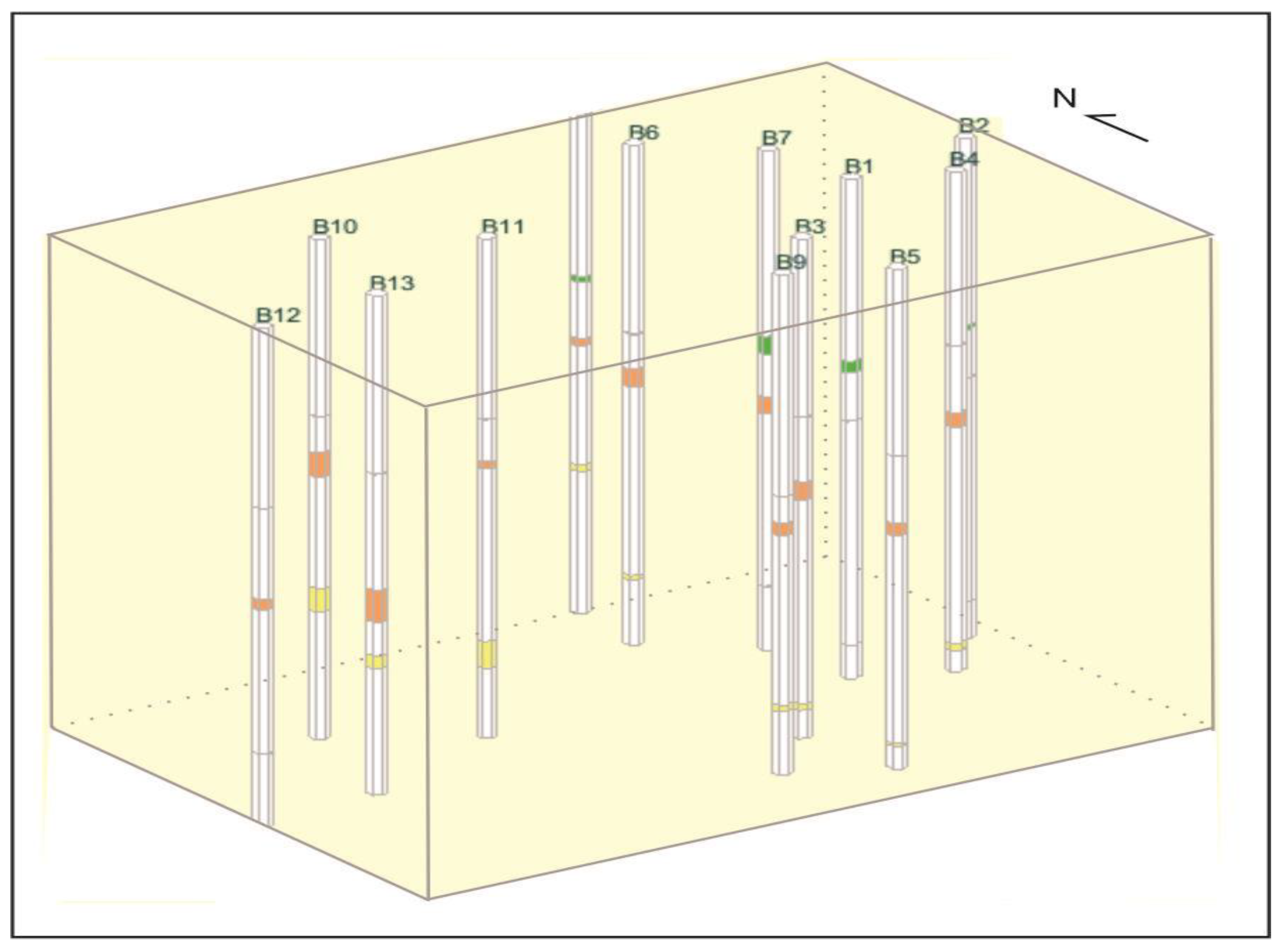
Figure 3.
Accuracy of validation when eigenvalue-k=5, 6, and 7, respectively. .
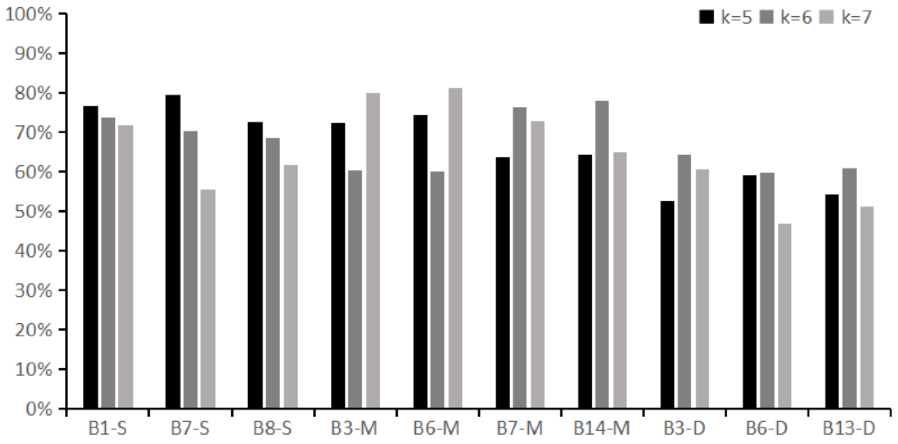
Figure 4.
Effect of trainset enhance in Shallow Layer, Middle Layer, and Deep Layer.
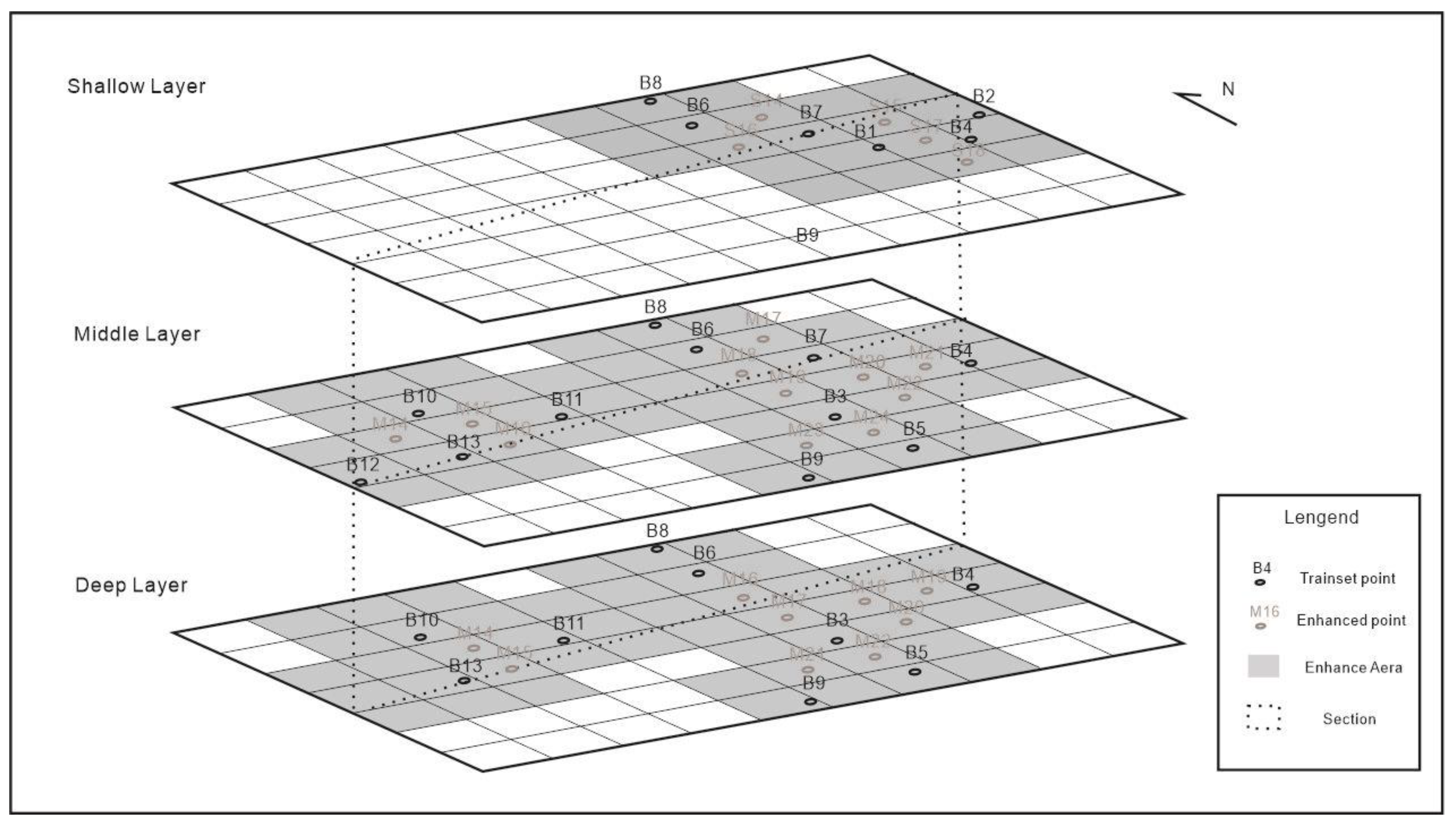
Figure 5.
Compare of the aquitard distribution in the Section.
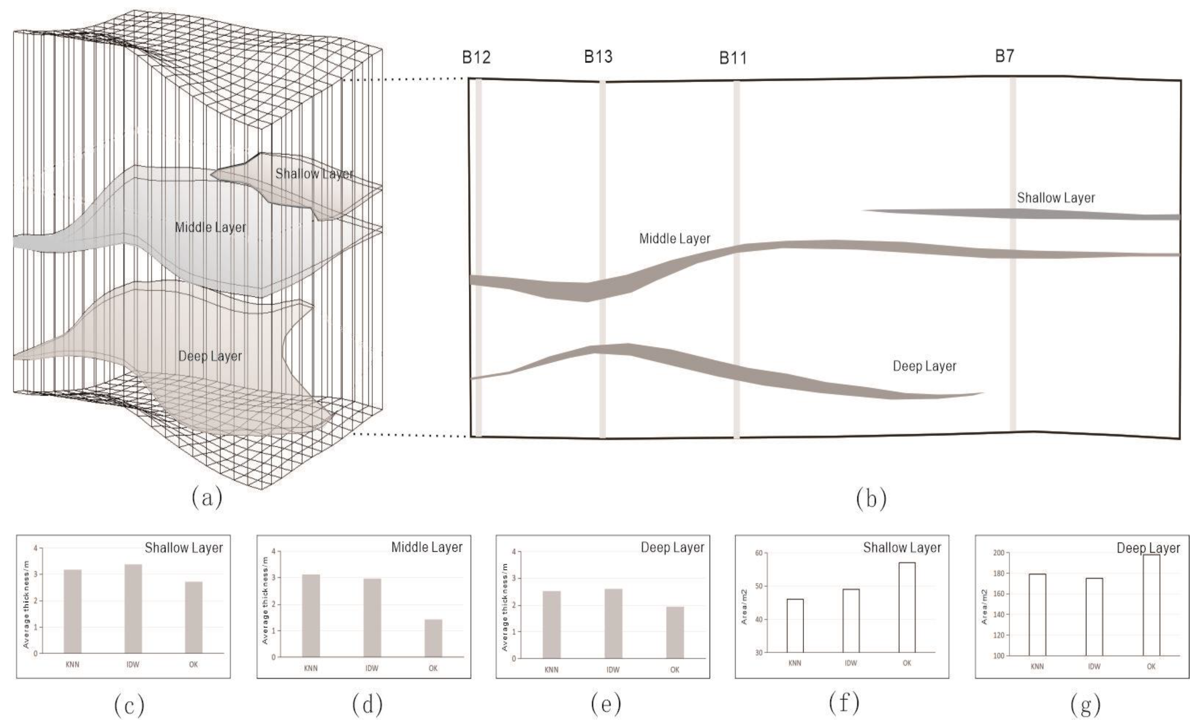
Figure 6.
Calculated A∙ΣM and it’s deviation in (a) the Shallow layer; (b) the Middle layer; (c) the Deep layer.
Figure 6.
Calculated A∙ΣM and it’s deviation in (a) the Shallow layer; (b) the Middle layer; (c) the Deep layer.
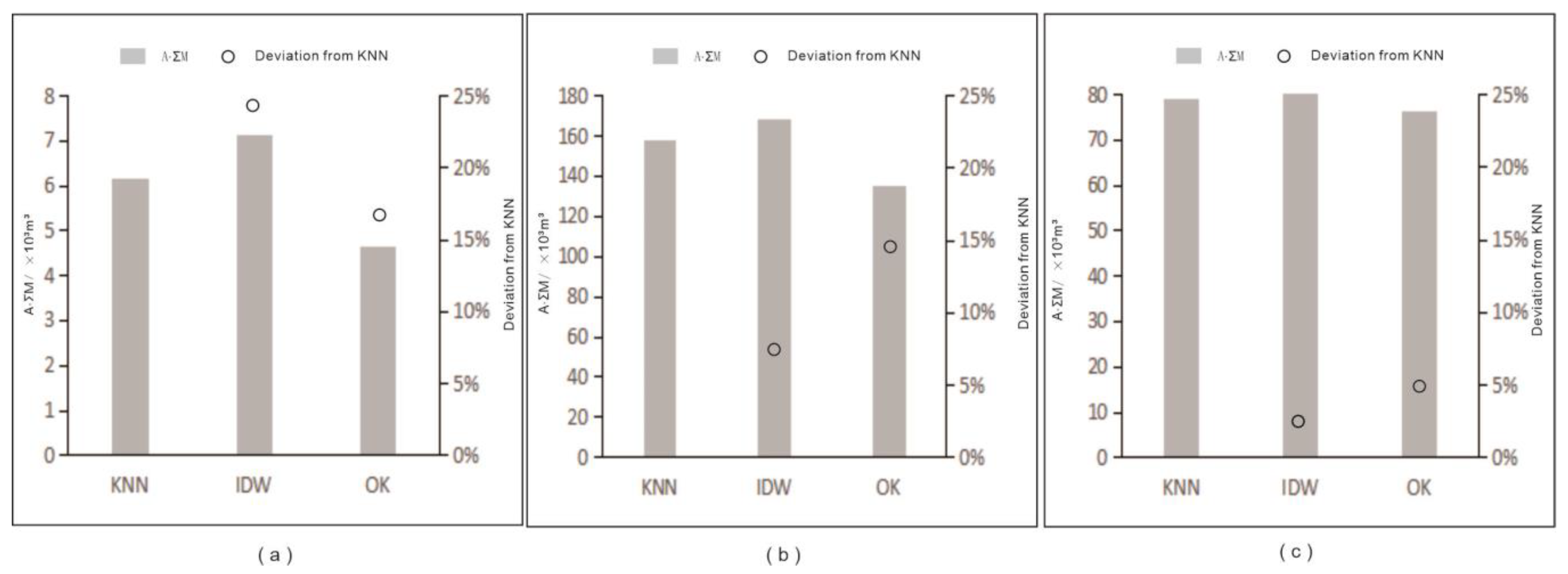

Table 1.
Different spatial interpolation algorithms predict accuracy.
| Layer | Method | MAE | MSE |
|---|---|---|---|
| Shallow Layer | KNN | 0.052 | 0.005 |
| IDW | 0.068 | 0.007 | |
| OK | 0.072 | 0.007 | |
| Middle Layer | KNN | 0.053 | 0.005 |
| IDW | 0.064 | 0.006 | |
| OK | 0.063 | 0.006 | |
| Deep Layer | KNN | 0.051 | 0.005 |
| IDW | 0.058 | 0.006 | |
| OK | 0.061 | 0.006 |
Disclaimer/Publisher’s Note: The statements, opinions and data contained in all publications are solely those of the individual author(s) and contributor(s) and not of MDPI and/or the editor(s). MDPI and/or the editor(s) disclaim responsibility for any injury to people or property resulting from any ideas, methods, instructions or products referred to in the content. |
© 2024 by the authors. Licensee MDPI, Basel, Switzerland. This article is an open access article distributed under the terms and conditions of the Creative Commons Attribution (CC BY) license (http://creativecommons.org/licenses/by/4.0/).
Copyright: This open access article is published under a Creative Commons CC BY 4.0 license, which permit the free download, distribution, and reuse, provided that the author and preprint are cited in any reuse.


