
Submitted:
19 July 2024
Posted:
22 July 2024
You are already at the latest version
Abstract
Today, it is difficult to have a high-field nuclear magnetic resonance device (NMR) due to the high cost of its acquisition and maintenance. These high-end machines require significant space and specialist personnel for operation and offer exceptional quality in the acquisition, processing, and other advanced functions associated with detected signals. However, alternative devices are low-field nuclear magnetic resonance devices. They benefit from the elimination of high-tech components that generate static magnetic fields and advanced instruments. Instead, they used magnetic fields induced by ordinary conductors. Another category of spectrometers uses the Earth's magnetic field, which is simple and economical, but limited in use. These devices are called Earth Field Nuclear Magnetic Resonance (EFNMR). This device is ideal for educational purposes, especially for engineers and those who study nuclear magnetic resonance, such as chemistry or other experimental sciences. Students can observe their internal workings and conduct experiments that complement their education without worrying about damaging equipment. This article provides a detailed explanation of the design and construction of electrical technology devices for the excitation of atomic spin resonance using Earth's magnetic fields. Covers all necessary stages, from research to analysis, from simulation, assembly, construction of each component, and the development of comprehensive software for spectrometer control.
Keywords:
Earth's Field NMR
; NMR spectrometer
; EFNMR
1. Introduction
The history of nuclear magnetic resonance (NMR) has no single origin. Before the first NMR signal was made, a series of events laid the necessary theoretical and technological foundations. This section outlines the main achievements that led to the discovery of NMR and its expansion into fields such as chemistry, biochemistry, and medicine. The study of NMR requires knowledge of a wide range of scientific disciplines [1]. NMR is at the core of several basic sciences and has applications in medicine, materials science, food, and agriculture, among other fields.
The quantisation of nuclear spin angular momentum (Stern-Gerlach) and the discovery of the magnetic resonance method (Rabi) are outstanding experiments in the origin of NMR. Stern and Gerlach observed in 1936 the separation of silver atoms in a nonuniform magnetic field, demonstrating the quantisation of angular momentum [2]. In 1942, Gorter attempted to observe nuclear magnetic resonance in solid matter, but was unsuccessful due to long relaxation times and low measurement temperatures [1]. Rabi and co-workers developed a resonance method using a molecular beam and oscillating magnetic fields, allowing accurate measurement of magnetic moments [3]. Gorter suggested the idea of applying radiofrequency energy to Rabi’s method in September 1937. Despite fundamental contributions, the NMR process has not yet been fully understood or uniformly accepted in the scientific community.
Bloch and Alvarez developed a method to measure the neutron magnetic moment using the molecular beam resonance technique in 1940 [4]. During World War II, Rabi, Ramsey, and Purcell worked on radar systems, while Bloch focused on molecular and atomic beam experiments. In 1945, Bloch returned to Stanford to work on NMR techniques, visualizing it as a change in the orientation of a nuclear magnetic moment. Meanwhile, Purcell proposed to work on NMR detection based on energy transitions [5]. Both groups carried out carefully designed experiments and successfully detected NMR signals. The findings of Bloch [6] and Purcell [7] were published in 1946 and were awarded the Nobel Prize in Physics in 1952. In the first NMR experiments on bulk substances, the relaxation times turned out to be much shorter than expected. This marked a turning point in the development of NMR, revealing its unprecedented potential [8].
Regarding the measurement of NMR spectra using short radio frequency pulses and observing free induction decay (FID) signals, Bloch originally suggested the idea of exciting nuclear spins with RF pulses for the observation of NMR signals in 1946 [9]. However, it was Torrey who performed the first pulsed NMR experiment in 1950, introducing the concept of a rotating reference frame [10]. In the same year, Erwin L. Hahn discovered the spin echo by designing a pulse sequence. This finding demonstrated the feasibility of RF pulse excitation and data acquisition in an FID. However, T2 measurement using spin echo suffered from the effects of molecular diffusion [11]. Around the same time, Hahn described magnetization reversal by pulses and improved the accuracy of T1 measurements. The serendipitous discovery of the spin echo by Hahn in 1950 overcame the impact of pulse reversal. Subsequently, Carr and Purcell demonstrated a simpler spin echo sequence and minimized diffusion effects in T2 measurements [12]. Meiboom and Gill introduced phase shifts in 180 ° pulses, leading to the Carr-Purcell-Meiboom-Gill (CPMG) pulse sequence for the measurement of T2 and more complex experiments, highlighting the importance of phase relationships between pulses [13].
NMR needed a new theoretical framework to address relaxation. Bloch introduced the concepts of relaxation times of T1 and T2 in 1946 [9]. The Harvard group, which included Bloembergen and Pound, developed the "BPP theory", explaining the effects of motion in NMR [14]. NMR made it possible to measure the magnetic moment of nuclei with high precision, and the Stanford group was particularly interested in this application. During measurements of the magnetic moment of 14 with , they discovered the chemical change by chance [15]. They observed two signals in a 1:1 ratio, which implied that the cation and anion generated different resonance signals. This was confirmed by observing the same phenomenon in other compounds such as 19. The chemical shift depended on the compound and the magnetic field [16]. In those days, some discoveries like Knight’s discovery showed differences in the frequency of NMR signal between metals and their salts [17] and the observation of separate signals for non-equivalent protons in simple organic compounds. This breakthrough made it possible to identify the different protons of a molecule in the NMR spectrum [18]. Furthermore, the position of the OH group in ethanol was found to be temperature dependent, which was explained as a consequence of hydrogen bonding interactions [19]. These discoveries marked a milestone in NMR and were made possible by significant improvements in NMR equipment, such as the homogeneity of the magnetic field and the addition of tuning elements at the magnet poles. In addition, the field of dynamic NMR was opened by describing the averaging of chemical changes due to fast exchanges [20]. Herbert S. Gutowsky introduced the term "chemical shift" and created a correlation plot between chemical shifts and structural features. This had a major impact on NMR as a tool for determining the chemical structure of a compound [21].
High-resolution NMR showed that the chemically shifted signals split into several symmetric lines. Proctor and Yu obtained the first example of multiplicity in the resonance of 121 in a solution of [22]. They attributed the splitting to incomplete cancelation of dipole-dipole interactions between the 121 and 19 nuclei due to restricted rotation. Gutowsky et al. found similar cleavages in fluorophosphorus compounds [23]. Purcell and Ramsey developed a theoretical explanation of the phenomenon in terms of scalar coupling between nuclei through chemical bonds. It was found that the expected splitting can be averaged by rapid chemical exchange.
The discovery of dynamic nuclear polarisation (DNP) by Albert W. Overhauser in 1953 challenged the theories of thermodynamic equilibrium by transferring the spin polarisation of electrons to the nuclei [24]. The DNP, experimentally verified, allowed significant changes in nuclear spin polarization due to perturbations in electron spins [25]. In 1955, I. Solomon used the term "nuclear Overhauser effect" (NOE) to describe changes in signal intensity in a two-spin system. Although experimentally confirmed, it took more than a decade for it to be recognized as a useful tool in NMR structural analysis [26].
The pioneers of NMR developed and built their own spectrometers. Initially, they used existing magnets, such as Bloch’s at Stanford and Purcell’s at Harvard. Although the early NMR apparatus was rudimentary, efforts were made to improve the homogeneity of the magnetic field. Steel parts (called "shims") were added and electrical coils were implemented to compensate for unwanted gradients. In addition, the agitation of the sample and the spinning speed improved the resolution of the spectra. With the discovery of chemical shifts and scalar coupling, the NMR technique reached maturity and was successfully applied to solve chemical problems. Thus, the focus of NMR shifted from solids studies to solution studies. Rapid development of NMR applications would not have been possible without the availability of commercial spectrometers. Varian Associates was the first company to market them [27]. NMR was initially secondary, but Varian reinvested profits from the core business in NMR research and development. The first high-resolution spectrometer, HR-30, was introduced to the market in 1952 [28]. Despite some difficulties, it was used to collect chemical data on known compounds. NMR has established itself as a valuable tool for structural analysis. Technical improvements were made, such as increasing the magnetic field strength and homogeneity of the magnet. More advanced models were introduced, such as the HR-40, HR-60 and HR-100. In 1961, Varian introduced the A-60, an easy-to-use spectrometer with a field/frequency locking system. Tetramethylsilane (TMS) was adopted as the internal reference standard and the chemical shift scale () with TMS at 0 ppm was adopted as recommended by IUPAC in the 1970s [29].
Improvements in NMR instruments have favored the development of new applications, especially in the structural analysis of organic compounds. In the 1950s, the capability of NMR to characterize steroids and other biomolecules was demonstrated. Martin Karplus established empirical correlations on the basis of NMR spectra, laying the foundation for conformational analysis. Furthermore, paramagnetic systems were investigated and dual resonance and 13 spectroscopy techniques were developed. Despite technical challenges, 13 data were successfully obtained and significant improvements were observed with the use of 1 decoupling and the application of nuclear saturation transfer effects (NOE). These advances allowed for the investigation of more dilute samples and the correlation of the 13 data with the molecular structure. Low sensitivity has always been a challenge in NMR spectroscopy. In the 1960s, the time-averaging method was introduced to improve the signal-to-noise ratio. However, data acquisition was slow and complicated. In 1966, Anderson and Ernst developed the Fourier transform NMR (FT-NMR) technique, which allowed spectra to be obtained more quickly and efficiently. This revolutionized NMR and opened up new possibilities in the study of chemical reactions and other processes. Richard Ernst received the Nobel Prize in Chemistry in 1991 for his breakthrough. NMR fever spread rapidly, and from the mid-1950s, JEOL and Hitachi in Japan and Perkin-Elmer Corp. in England began marketing NMR spectrometers. In 1957, Trüb-Täuber launched the KIS-1 NMR spectrometer on the market, followed in 1963 by the KIS-2 [30]. In 1965, Günther Laukien acquired the NMR department of Trüb-Täuber and founded Bruker Spectrospin [31]. Bruker’s first major success was the HXF-90 in 1967, followed by the addition of an FT attachment to the HX series spectrometers. Surprisingly, Varian failed to appreciate the potential of Fourier transform NMR discovered by its own employees after 20 years of market leadership.
An obvious option to increase the sensitivity of NMR was the use of higher magnetic fields. In 1962, Varian developed a prototype 200 MHz superconducting NMR spectrometer. Two years later, the first HR-220 (1, 220 MHz) spectrometer was installed. This improvement represented another milestone in the NMR timeline. Subsequently, Oxford Instruments built a 7.5 T magnet (320 MHz for (1), which served as the basis for the creation of the first superconducting FT-NMR spectrometer at 270 MHz. Subsequently, periodic increases in the frequency of 1 were achieved, reaching 600 MHz in 1987. This made it possible to address more challenging problems, especially in biochemical systems. This research spurred the development of technologies that led to 750 MHz, 800 MHz, 900 MHz and even 1 GHz spectrometers in 2009. In 2015, JEOL raised that frequency limit to 1.02 GHz, and in April 2019, Bruker announced a record with the world’s highest magnetic field in NMR: 25.9 T (1.1 GHz for 1).
In the 1970s, two-dimensional (2D) NMR was developed thanks to the proposal of Jean Jeener and the advances of Richard R. Ernst [32]. The technique consists of a sequence of pulses and waiting times that allow obtaining a 2D spectrum showing the relationship between the nuclei of a spin system at different time periods [33]. This innovation revolutionized NMR spectroscopy and laid the foundation for numerous subsequent variations. The implementation of 2D NMR required advances in hardware and software, as well as improvements in computational capacity. In the 1980s, its potential in liquids and solids was exploited, making it possible to obtain structural and dynamic information on complex systems [34]. Indirect detection methods, such as HSQC (Heteronuclear Single Quantum Correlation) [35] and HMQC (Heteronuclear Multiple Quantum Correlation), increased sensitivity [36]. A strategy for structural analysis was established on the basis of the combination of different spectra and correlations. The theory and introduction of technical innovations facilitated the design of pulse sequences and improved the performance of experiments. The application of NMR in biochemistry was recognized early, with information on structures and configurations/conformations of biological substances being obtained as early as the 1950s. In the 1980s, NMR spectroscopy underwent significant instrumental and methodological advances. 2D NMR techniques revolutionized the structural characterization of biopolymers by allowing the determination of coupling bonds and interatomic distances. The development of computational methods and molecular dynamics simulations was crucial. In 1982, complete assignment of the spectrum of one protein was achieved, followed by determination of the three-dimensional structure in solution of another protein in 1984. Expansion to additional dimensions and the use of pulsed-field gradients led to high-quality 4D spectra.
Advances in structural biology studies come from improvements in instrumentation and methodological tools. NMR spectrometers up to 1.1 GHz provide higher resolution and sensitivity. Hyperpolarization and improved probe design allow for more intense signals and the determination of three-dimensional structures with small amounts of sample. In addition, novel methods such as residual dipole coupling (RDC), TROSY spectroscopy, and fast NMR acquisition techniques have been developed [37]. Non-uniform sampling (NUS) also accelerates acquisition by omitting part of the data [38]. These advances, together with the use of computational methods, have made NMR a powerful alternative for the determination of the structure of biopolymers, especially for the study of dynamic processes [39].
In the first attempts to apply NMR to living systems, limitations were encountered due to the primitive stage of the technique. However, a real breakthrough in medicine was achieved with the implementation of high-intensity spectrometers in the 1970s. Methodological improvements were developed, such as water suppression and spin echo techniques, which allowed the metabolic study of tissues and cells. The introduction of high-field superconducting magnets and the high-speed spinning technique (HRMAS) opened up new possibilities in NMR medicine [40]. Currently, magnetic resonance imaging is used in pathological diagnosis and biofluid analysis, as well as in vivo studies together with magnetic resonance imaging (MRI) [41].
From the first steps of NMR, developers and scientists sought to improve the homogeneity of the magnetic field to obtain narrower peaks. In 1971, Lauterbur discovered that the application of inhomogeneous magnetic fields would allow signals to be identified according to their spatial coordinates. Using linear gradients in three orthogonal directions, Lauterbur succeeded in encoding spatial information and obtaining two-dimensional images. The first NMR image was published in 1973 [42]. Shortly thereafter, in 1977, P. Mansfield described an alternative called "echoplanar imaging" (EPI) that allowed spatially encoded data to be obtained in a single radiofrequency excitation [43]. These advances in magnetic resonance imaging have revolutionized clinical diagnosis by providing noninvasive tools and integrating anatomical and spectroscopic images. fMRI and DTI techniques provide functional and diffusion information, respectively, and are especially useful for studying brain and cardiac activity. These advances would not have been possible without the contribution of computational and data-processing techniques. Solid-state NMR (ssNMR) developed more slowly than solution NMR because of the broad signals of solid materials. However, advances have been made with the introduction of Fourier transform spectrometers and three main methods: magic angle sample spinning, homonuclear decoupling, and cross-polarization [44]. These advances in instrumentation and software have allowed the application of ssNMR to a wide range of samples, including biological membranes, membrane proteins, tissues, and polymers [45]. ssNMR continues to be a growing field [46].
The first Earth’s field NMR (EFNMR) was performed in 1954 [47,48], it was a curiosity, and the main use was for geophysical magnetometry [49] or simply a low-cost demonstration of magnetic resonance principles. Despite its low field, it continues to attract the attention of researchers and engineers not only because of its rarity as a physical phenomenon but also because of certain low-field results that are difficult to obtain in high field, such as the inflection obtained in the dependence of the inverse of T1 below 0.01 T of the signal detected in some tissues[50], as well as other applications encountered [51,52]. The strength of the Earth’s magnetic field is very low. It is still possible to obtain narrow NMR lines and a high signal-to-noise ratio with acceptable spectral resolution. In the 1960s, Béné and colleagues demonstrated that EFNMR could measure the J-coupling of nuclear elements [53]. Because high homogeneity and stability can be achieved successfully in low fields, experiments have proven that many important spin multipliers can be studied in low fields. Chemical shift differences have recently been demonstrated to be measured even in inhomogeneous low magnetic fields [54].
This device presents several potential applications. One significant application is the precise measurement of the chemical shift of hyperpolarized xenon-129 in the Earth’s magnetic field, achieving a precision similar to high-field measurements [55]. Furthermore, 1H and 19F EFNMR spectra can be acquired with frequency resolutions nearly two orders of magnitude better than those obtainable with high field high-resolution NMR [56]. Another application of a break-through is the observation of heteronuclear J-couplings using the classic COSY experiment [57], and more recently the first observation of homonuclear proton J-couplings in the Earth’s magnetic field, previously considered impossible [58]. In the realm of condensed matter physics, low-field NMR allows for high-resolution spectra in solids by minimizing the line broadening caused by dipole–dipole interactions in high fields [59]. Moreover, low magnetic fields allow observation of ’forbidden transitions’, providing unique information that is not detectable at high magnetic fields Kohl et al. [60].These applications highlight the versatility and potential of NMR in various scientific fields.
2. Motivation and Objectives
NMR has proven to be an exceptionally valuable tool in a variety of disciplines, from diagnostic medicine to chemical and biological research. However, most current NMR spectrometers require intense magnetic fields, which limits their use to specialized laboratory environments. The development of an NMR spectrometer that can effectively operate using the Earth’s magnetic field represents a significant pedagogical shift. This advancement could revolutionize the educational application of NMR, enabling its integration into specialized NMR courses within the curriculum.
Current NMR equipment is prohibitively expensive for many institutions, especially those in developing countries and organizations with limited budgets. Using the Earth’s magnetic field, a more accessible NMR spectrometer can significantly reduce costs and lower barriers to access, allowing a much broader range of researchers to use this valuable tool. However, its use is currently limited to educational purposes.
The potential applications of an Earth field NMR spectrometer extend beyond traditional laboratories. There are numerous situations where access to conventional NMR equipment is challenging or impossible, such as field research, low-resource environments, or remote geographic regions. An Earth field NMR spectrometer could enable on-site analysis, provide real-time data, and eliminate the need for sample transportation. As it can be transported, this has allowed us to carry out extensive research of diffusion in explorations of antartic ice and groundwater [61] [62].
Research into an Earth field NMR spectrometer also has the potential to deepen our fundamental understanding of nuclear magnetic resonance. By working with much lower magnetic field intensities than usual, we can gain new insights into the underlying principles of NMR and uncover previously unobserved behaviors and properties. This additional knowledge could open new avenues for research and application beyond the purely educational purposes mentioned above.
The main objective of this paper is to design and construct an NMR spectrometer that uses the Earth’s magnetic field as a constant magnetic field to operate. In addition, the aim is to design systems that can generate acceptable and useful results under various operating conditions. To evaluate the efficiency and effectiveness of the Earth-field NMR spectrometer, its results will be compared to those of conventional NMR spectrometers. One of the main advantages of Earth-based NMR spectrometers is the ability to use conventional NMR spectrometers in situations where conventional NMR spectrometers cannot be used. Consequently, spectrometers are designed and developed so that they are as portable, durable, and user-friendly as possible to be used in a wider range of environments. Data collected by Earth’s field NMR spectrometers must be processed and analyzed. Herein, we have developed robust and user-friendly software systems to manage this process, simplify data interpretation, and allow users to extract the maximum value from the results obtained.
3. Principle of Operation and General Aspects
Nuclear magnetic resonance (NMR) is a physical phenomenon in which atomic nuclei in a magnetic field absorb and re-emit electromagnetic radiation. This process allows for an investigation of the physical and chemical properties of the nucleus itself and its surrounding environment.
Nuclear spin is a fundamental property of atomic nuclei related to the number of protons and neutrons they contain. Some nuclei with specific properties, such as 1H (protons), 13C, 15N, and 31P, are NMR active, which means they have a nonzero spin quantum number. This spin imparts a magnetic moment to them, turning them into tiny magnetic bars.
In an NMR experiment, an external magnetic field, , is applied. The magnetic moments of the nuclei will align with the external field, but in quantum mechanics this alignment is quantized, Figure 1. This means that nuclear spins can align in specific orientations dictated by their spin quantum number (). For example, a nucleus with a spin quantum number of 1/2 (such as 1H or 13C) has two possible spin states in an external magnetic field: "spin-up" () or "spin-down" (). These states have different energies, with the spin-down state being the higher energy state.
The constant that relates the Larmor frequency to the applied magnetic field is called the gyromagnetic constant, which for 1H is 42.574 MHz/T. The energy levels produced can be quantified as follows,
where is the energy level of the atom I, h is Planck’s constant, is the quantum spin number, is the gyromagnetic constant, and is the external magnetic field. These two energy levels are known as the alpha and beta states. For the hydrogen atom, the energy levels () for a 600 MHz (14.1 T) spectrometer are around J. The thermal energy () that determines the population ratio of a partition distribution is around J. Thus, the population associated with this energy state can be calculated as,
The population ratio for the different levels can be estimated by subtracting the energy levels and dividing them by the sum of the two:
Equation 3 reveals that for a 600 MHz spectrometer at 288 K, the fraction of populations is around , therefore, only a small fraction will have a net magnetization ,
where N is the total number of populations, is the molar concentration of the nuclei considered, V is the volume of the sample, is the external magnetic field, and R is the universal gas constant.
is the projection on the Z-axis parallel to the external magnetic field, referred to as the polarization in of all spins, which defines the signal intensity in resonance. These energy levels are called Zeeman energy levels and determine the magnetization parallel to the external magnetic field (Figure 2). In NMR, a radiofrequency (RF) pulse is used to perturb the nuclear spins from their equilibrium state. If this RF pulse matches the Larmor frequency (a condition known as "on resonance"), the nuclear spins can absorb this energy and "flip" from the lower-energy state to the higher one. Once the RF pulse is turned off, the system will return to equilibrium, a process known as relaxation. During this process, the nuclei will emit the absorbed energy in the form of an electromagnetic signal, which can be detected and used to generate the NMR spectrum (Figure 2). The population difference between the alpha and beta states is very small, but sufficient to produce an observable NMR signal, as explained previously. The system is in equilibrium when the ratio between the populations of the alpha and beta states remains constant. In this state, there is no net magnetization in the transverse plane (x-y). A short and intense burst of radiofrequency (RF) radiation, called an RF pulse, is applied perpendicular to . If this RF pulse matches the Larmor frequency (the resonance frequency of the spins), the nuclear spins can absorb this energy, causing a 90o flip of their alignment with into the transverse plane (x-y). This generates a net magnetization in the transverse plane, creating a non-equilibrium state (Figure 2). It is a natural process based on the minimization of energy and maximization of entropy; see Table 1. In NMR, this natural process is observed by minimizing the spin energy and maximizing the nuclear spin phase.
The variables involved in the spin perturbation process are the intensity of the radiofrequency pulse (), the phase value, and the duration of the pulse (). The flip angle of the Z-axis over the X-Y plane is determined as = .
After turning off the RF pulse, the system does not remain in a non-equilibrium state. The spins will gradually return to their equilibrium alignment along the Z-axis, a process known as relaxation. Relaxation occurs in two distinct processes: longitudinal relaxation (or T1) and transverse relaxation (or T2).
T1 relaxation is an enthalpic process where a net electromagnetic emission occurs, producing a detectable signal as the system transitions from a nonequilibrium state to equilibrium. Also known as spin-lattice relaxation, T1 relaxation is the process in which the net magnetization vector in the transverse plane returns to the Z-axis. This process is associated with the energy released by the spins as they return to equilibrium, causing the nuclei to revert to their original energy states. The relaxation time T1 is a measure of how quickly this process occurs. The physical model of relaxation can be mathematically expressed as follows.
Equation (3) shows what is called a coherent transition where photons are emitted, resulting in a detectable signal. The relaxation is an entropic process in which the detectable signal has a phase among the different nuclear spins, producing relaxation in the XY plane. Also known as spin-spin relaxation, relaxation is the process by which the spins in the XY plane dephase (i.e. lose their coherence). During this process, the transverse magnetization decays to zero as a result of interactions between the spins. The relaxation time is a measure of the rate at which the transverse magnetization decays.
This is the classical description of nuclear magnetization behavior, developed by Bloch in his vector model in the presence of an external magnetic field and following excitation by an RF pulse. These equations, named after Felix Bloch, model nuclear spins as a bulk magnetization vector and describe their precession and relaxation behavior. Although Bloch’s model is incredibly useful and has greatly contributed to our understanding of NMR, it has several limitations.
- Lack of quantum effects: Bloch equations are classical and do not account for quantum mechanics effects. For example, they do not consider that the spin state of a nucleus is quantized.
- Assumption of a homogeneous magnetic field: The equations assume a perfectly homogeneous external magnetic field. In reality, magnetic fields often exhibit inhomogeneities, which can lead to various effects not covered by Bloch equations.
- Assumption of instantaneous excitation: The equations assume that the transition from equilibrium to non-equilibrium (during the RF pulse) is instantaneous. In real scenarios, the RF pulse has a finite duration, and its effect on the spin system might not be as abrupt as assumed by Bloch equations.
- Neglect of multiple spin interactions: Bloch’s model does not consider the interaction of different spins with each other (spin-spin interactions), which can lead to more complex phenomena such as relaxation and spin-spin coupling.
- Assumption of large spin ensembles: Bloch equations consider the behavior of a spin ensemble, thus providing average values. They do not provide information on the behavior of individual spins within the ensemble.
- Simplification of relaxation processes: The equations simplify relaxation processes ( and ) to single exponential decays, whereas in reality these processes can involve multiple components with different relaxation times.
Despite these limitations, the Bloch equations remain a fundamental tool in understanding and interpretation of NMR, offering a simplified and efficient description of many phenomena encountered in this field. However, for a more detailed understanding of complex NMR phenomena, it is necessary to resort to quantum mechanical descriptions or more advanced models.
Nuclear Magnetic Resonance in the geomagnetic field is known as Earth’s Field NMR (EFNMR), a special case of low-field NMR. When a sample is placed in a uniform magnetic field, nuclei with non-zero spin experience resonance at specific frequencies. This document exclusively covers Proton Nuclear Magnetic Resonance (NMR), primarily involving the 1H isotope.
4. Materials and Methods
This document exclusively covers proton NMR, mainly involving the 1H isotope. In the Earth’s magnetic field, which is around 45000 nT depending on the location, the 1H isotope has a Larmor frequency of approximately 2 kHz and generates a very weak signal of a few microvolts.
Figure 3 shows the block diagram and the complete architecture of this EFNMR spectrometer. The polarizing coil assembly includes two receiver coils (Rx) that are connected in an antiparallel configuration to cancel out environmental noise. The current flow through the polarizing coil is managed by a regulated power supply, controlled by a polarizing switch. The sample is placed inside one of the coils and the outputs of both Rx coils are fed into a differential amplifier through a relay-controlled switch.
Given the small magnitude of the resonance signal, on the order of microvolts, signal amplification is essential before further processing. Therefore, the signal is channeled through a fixed gain ultra low noise differential amplifier, a low noise amplifier, and then to a bandpass filter, with a cutoff frequency around the Larmor frequency, thus eliminating unwanted noise and frequencies.
The filtered signal undergoes an additional amplification stage before being acquired by the microcontroller -ADC. Finally, signal processing is implemented on these data to extrapolate and visualize the desired magnetic resonance information.
4.1. CAD Desing and 3D Printing
3D printing is a very useful tool for prototyping. It allows for the fabrication of parts designed using CAD programs. In this project, 3D printing has been used to manufacture the cylinders on which the coils are wound and the base that holds them, as well as other complementary parts that will be discussed below. To design the parts used in this project, the CAD program was used. This software is a comprehensive 3D design tool that combines parametric modeling, rendering, simulation, and computer-aided manufacturing functions in a single integrated package.
The first part designed was the cylinder of the polarizing coil. This cylinder has a height of 145 mm, an outer diameter of 90 mm, and an inner diameter of 80 mm. Two holes with a diameter of 2 mm were made 20 mm from the base to allow the coil wire to pass inside the cylinder. The second part designed was the cylinder of the receiving coils. This cylinder has a height of 140 mm, an outer diameter of 32 mm, and an inner diameter of 28 mm. Similarly to the polarizing coil cylinder, this cylinder also has two holes made 20 mm from the base, but this time with a diameter of 1.5 mm to allow the coil wires to pass inside the cylinders. Figure 4 shows the CAD design of the polarizing coil and the receiving coil cylinders.
The three coils are aligned by means of a base that has grooves of 15mm deep and a width equivalent to the thickness of the walls of the cylinders where each of the coils are fitted, and this same base aligns the wires of connection of the coils to match the connections of the printed circuit.
In order to be able to modify the inclination of the coils, and to be able to align the terrestrial magnetic field in an optimal way, a support was designed, which holds the excitation coil and allows one to modify the angle with the base. The base of the equipment has a curved surface where the support can slide and two fixing screws, which allow to secure the mounting in the desired position. The fixing screws used are plastic, so there is no need for any metal component that could alter the magnetic field near the coil. Figure 5 shows the CAD design of the various parts and the assembled model.
Once the design of all parts in CAD is completed, the files are transferred to G-code translator. This kind of software is a sophisticated 3D model preparation software that enables the configuration and optimization of printing parameters. This process is essential before generating the G-code file required for 3D printing. The final result after CAD design and printing is shown in Figure 6.
4.2. Polarizing coil
The polarizing coil temporarily creates a polarizing magnetic field . This field quickly turns off, leaving the magnetization instantly perpendicular to the Earth’s magnetic field around which precession begins [63,64]. The polarizing coil and its supporting structure must not contain any ferromagnetic material. Naturally, the Earth’s field is very homogeneous, and if there is any ferromagnetic material near the coil, it will change the uniformity of the field, causing magnetic field inhomogeneities. To properly use the device during normal experiments, the entire system should be free of electromagnetic interference due to the weakness of the detected signal. However, since the goal of this project is to design a benchtop device, it has been designed to be robust under electromagnetic stress conditions. The purpose of the polarizing coil is to produce a magnetic field much greater than the Earth’s magnetic field. To polarize the sample, a current of approximately 10 A is passed through the coil for 10 seconds. Therefore, the wire for winding the polarizing coil must have a large enough cross section to avoid heating while carrying this current. The specifications chosen for the polarizing coil are given in Table 2.
The polarizing coil cylinder is wound on a commercial PVC (vinyl polychloride) tube.The polarizing coil is placed in the center of the coil holder which is provided with holes for passing the connections to the PCB, placed under this holder. The base, inclination part, and coil support are made of PETG, avoiding the use of metal. The tilt platform should form an angle close to 50 ° relative to the base. The angle ensures that when is turned off, the magnetization is perpendicular to the Earth’s field immediately prior to signal detection. This geometrical arrangement maximizes the strength of the signal. The Earth field in southern Spain (University of Almeria) has an inclination of 50.57° and a declination of 0.59°.
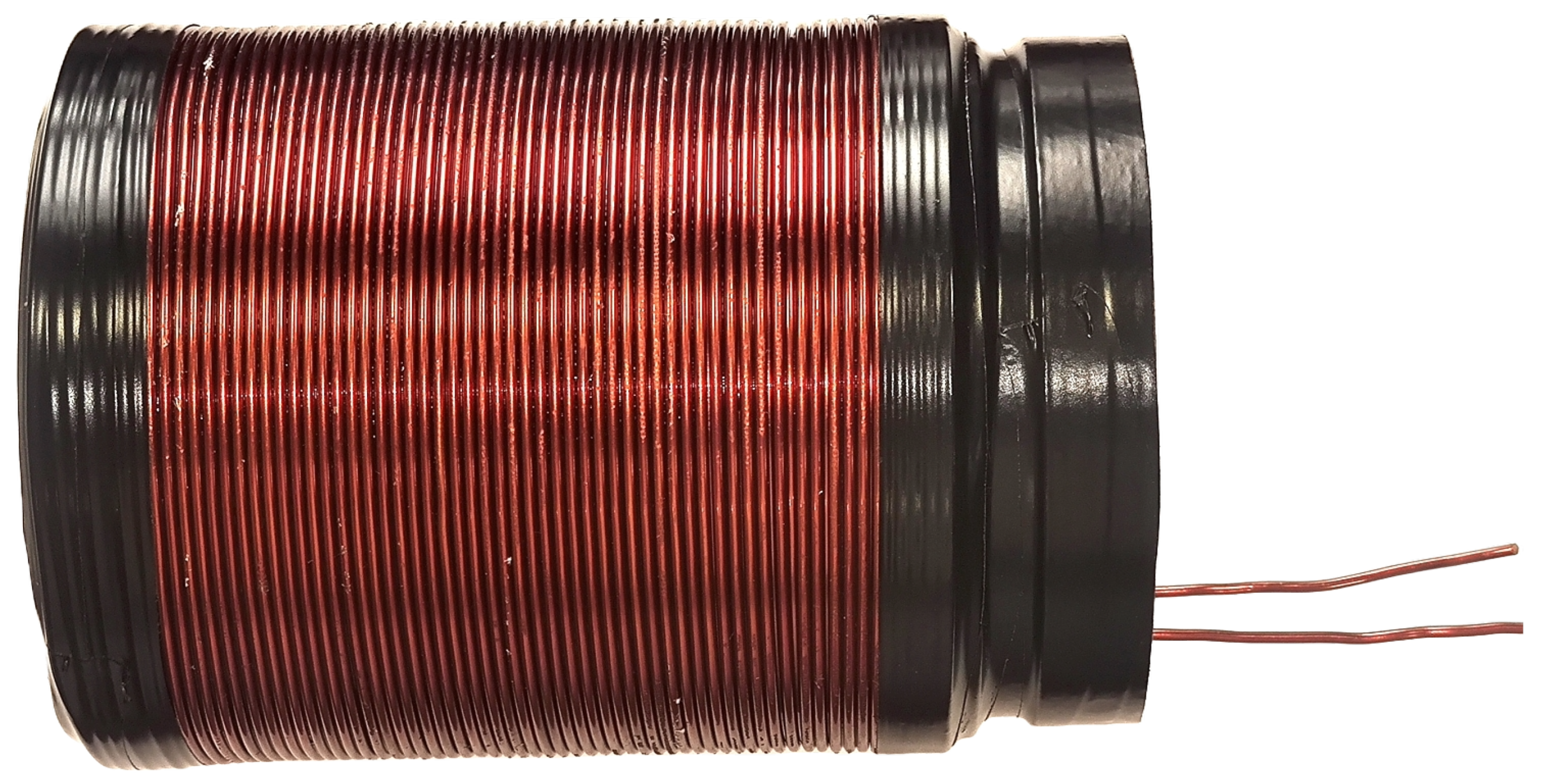
Figure 7.
Wounded polarizing coil.
4.3. Receiver Coils (Antenna)
The receiving coils () are responsible for collecting the signal from the polarized sample in precession. The signal is extremely low, requiring many iterations of the experiment to increase the signal-to-noise ratio (SNR). This process is known as signal averaging. The main problem affecting this device is noise, which is why the coils have been designed to minimize it. In addition to signal averaging, two nearly identical sensor coils are used to address this issue and maximize the SNR.
The two coils are wound in series but in opposite directions and placed on the same surface to cancel out noise (Figure 8). To receive the signal, the sample is placed in only one of the coils because if it is placed in both coils, the produced signals will cancel each other out, resulting in no signal being received at the output.
The most important requirement for correct winding is that both coils must be as identical as possible to perfectly cancel out environmental noise. This is called common-mode rejection and can be achieved if the number of turns is equal for both coils and the wire is not twisted at any point during winding. To verify the similarity of the coils, one method is to weigh the coils before and after winding. As with the polarizing coil, the material used for the cylinders on which the receiving coils are wound is a commercial PVC pipe.
As mentioned earlier, the device was designed to operate using the Earth’s magnetic field, so any nearby ferromagnetic material must be avoided. Metallic objects such as copper, aluminum, and brass should also be kept away from the coil to avoid induced eddy currents when is quickly turned off.
The wire cross section is also an important parameter. With a thin wire, we have more turns and a stronger signal, but it also has higher resistance and therefore more Johnson noise , which we do not want. On the other hand, with a thick wire, we have fewer turns and a weaker signal compared to a thin wire, but the noise is lower and the quality factor can be higher. The thermal noise follows the resistance relationship in volts:
where is Boltzmann’s constant (J/K), T is the temperature in K, R is the resistance and is the bandwidth. The specifications of the receiving coils are summarized in Table 3.
To verify the proper functioning of the receiving coils, some preliminary tests were conducted. The coils were placed inside the polarizing coil, and a sinusoidal signal was applied to the polarizing coil using a function generator (Figure 10). This induces a sinusoidal wave in both receiving coils of the same amplitude and approximately 180 degrees out of phase with the excitation source. Both waves cancel each other out, resulting in an almost null signal. All these signals were measured and analyzed in Matlab (Figure 11).
4.4. Power Circuit
This circuit is responsible for turning the power supply of the polarizing coil on and off with a signal from the microcontroller. This circuit had to be carefully designed because, for the experiment to work correctly, the coil needs to discharge as quickly as possible, and consequently, so does the magnetic field it generates. Therefore, no switch can be used to turn off the polarizing coil. Mechanical relays could be used to turn the polarizing coil on and off, but they are not the best option due to several disadvantages. The relay operates like a basic switch and can produce an electric arc when it turned off, as the coil has high induced voltages. Relays also have a short lifespan and take a few milliseconds to switch. In our case, the polarizing coil needs to be turned on and off within microseconds. Therefore, the simplest solution to this problem is to use a power MOSFET with a shorter switching time.
The MOSFET used is the IPD090N03L. The maximum allowed collector-emitter voltage is 30 V, and the base-emitter voltage is 20 V. The maximum current it can drain is 40 A. The IPD090N03L has an extremely low internal on-resistance of 0.009 . The positive power supply of +12 V is connected to one terminal of the polarizing coil, while the other terminal is connected to the MOSFET’s collector. The MOSFET emitter is connected to the ground. The MOSFET is operated by the microcontroller, through a specific driver that boosts the voltage and current provided by the microcontroller to levels that ensure fast switching with the least amount of losses possible. Because high voltages are induced during the switching of the MOSFET, it is important to include a diode that absorbs these surges without damaging the MOSFET. Given the low resistance of the MOSFET, the amount of heat generated during switching can be dissipated by the PCB itself. The complete circuit schematic can be seen in Figure 12.
4.5. Receiver Circuit
The signal detected by the receiver coils is extremely small (on the order of microvolts). This signal needs to be converted by the microcontroller ADC to be processed by a computer, but it needs to be adapted; for this purpose, six different stages are designed as shown in Figure 13.
First stage is a capacitors block. These capacitors act as tuners and are responsible for enhancing the signal before it reaches the instrumentation amplifier. This is achieved by placing these capacitors in parallel with the receiving coil. The value of the capacitor can be found using the resonant frequency formula 10.
The frequency f is adjusted (adjusting C) to be as close as possible to the Larmor frequency of the proton, which is approximately 2 KHz. Here, L is the combined inductance of both coils and its value is 5.12 mH. The optimal value of the tuning capacitor is 1.13 F. This value is approximated by 1 F and two 56 nF.
The second stage is a double relay controlled through the microcontroller that connects the output of the coils. The normal position of the relay switches is open. Each end of the receiving coils is connected to one of the relay switches, while the common point of the two coils is connected to the ground. When the microcontroller sends a signal to the transistor, it connects the relays to the +5V power supply, causing the relay switches to activate, allowing the signal from the receiving coils to pass to the instrumentation amplifier. The circuit is shown in Figure 14.
Third, there is an ultra-low-noise instrumentation preamplifier. An INA848 has been used, which is a high-precision instrumentation amplifier that requires no external components for a fixed gain of 2000. Since the signal is in microvolts, only low-noise amplifiers can be used. Both ends of the coils are connected to the input of the instrumentation amplifier, while the sample is placed in only one of the coils, as mentioned earlier. When the signal arrives, the signals from the two inputs of the instrumentation amplifier are subtracted, and the signal emitted by the proton is obtained.
The fourth stage is an amplifier stage, with gain 1000, built with one of the four operational amplifiers available in the OPA4189. In the fifth stage, signal filtering is performed, using the remaining three amplifiers to perform a band-pass filter of order 6, designed to attenuate the frequencies outside the range of interest for this application. Specifically, 1.8 kHz center frequency and a width of 1.5 kHz have been chosen. The filter response is shown in Figure 15
The last stage transforms the signal to differential mode and adapts the impedance values to those expected by the 16-bit ADC incorporated in the microcontroller. In this stage, the signal is shifted from referenced to GND to swing around , which is required to meet the input ranges of the ADC. Both the reference voltage and are supplied by a precision voltage reference, in this case a REF2025.
The differential mode used significantly improves the conversion by increasing the noise immunity. No gain is introduced at this stage, so the total system gain is 2000000. The complete input schematic is shown in Figure 14.
4.6. Adquisition Sequence
The quality of the data obtained is strongly dependent on the precise timing of the different stages involved in the process. By design, this device alternates between the excitation stage, in which the polarizing coil is involved, and the relaxation stage, in which the receiver coils are involved. In this case, the acquisition process is fixed, and the timing parameters and the number of repetitions can be configured at the beginning of each experiment.
At the beginning of each scan of the experiment, the microcontroller activates the current conduction to the biasing coil. After the excitation time () the coil is turned off. Once a preset time () has elapsed, which is necessary for the field of the biasing coil to discharge, the relay closes and the receiver coils are connected to the amplifiers. Digitization begins after a second period (), which ensures complete closure of the relay, the duration of which varies according to the number of samples required (). At the end of the sampling, the relay opens and waits for the relaxation time (). This process is repeated for the indicated number of times, improving the system’s ability to distinguish signal from noise.
4.7. Control and Communications
The control tasks of the equipment, the digitalization of the amplified and adapted signal in the previous section, and the communication with a computer are handled by an ARM microcontroller (STM32F373). This microcontroller has the required features for the correct operation of the unit, including a 16-bit resolution analog-digital converter and USB communications for sending the large number of samples that need to be acquired. Of course, it has diverse input and output pins, timers, and SPI and I2C communication ports among others. To enable USB communication, it is required to use a 72MHz clock frequency, obtained from an 8 MHz crystal and the internal PLL.
The required design is simple, having only the outputs corresponding to the activation of the polarizing coil and the relay, the analog inputs for the signal, and a communication port with the computer. The rest of the elements are auxiliary to achieve the correct operation of the instrument. Figure 17 shows the microcontroller section as well as the rest of the auxiliary elements of the circuit.
Since the coils need to be properly aligned with the terrestrial magnetic field, a 3-axis magnetometer has also been incorporated which is accessed by the microcontroller via the I2C bus. As the PCB is precisely aligned with the coils, it is convenient and practical to be able to use this magnetometer to adjust the position before starting the measurements, ensuring better results. The read values are visible from the program interface.
4.8. Computer Software
To ensure proper use of the unit, we developed basic control software in C#. This language for programing was chosen because it is driven by the extensive library support and the language’s ease of use, facilitating the enhancement and swift implementation of new experiments and functionalities. The main window (Figure 18) presents configurable experiment parameters, enabling the user to adjust the settings as required.
- The number of samples to capture, according to this number and taking into account the fixed sampling frequency, the duration of this period is indicated, corresponding to .
- Number of scans, or number of times the acquisition cycle will be repeated. Corresponds to the parameter N.
- Recovery time, or time required after acquisition until a new cycle starts. Corresponds to .
- Pulse time, or polarizing coil activation time. corresponding to .
Although the software is intended to test the functionality of the machine, the ability to model the noise has been incorporated, saving the results and allowing to improve the behavior in subsequent experiments. This function is performed by running one or more scans without introducing any sample. The frequency response (FFT) obtained will be stored in a file and used subsequently to suppress the background noise. The software also allows you to switch between the Fast Fourier Transform view (FFT) and the free-induction decay view.
5. Results and Discussion
In this paper, we successfully designed and built a complete assembly and electronic component EFNMR spectrometer from scratch. All parts, including the spectrometer framework, are manufactured with PETG material and 3D printing technology with CAD design and 3D printing to ensure the device’s robust and accurate structure.
The electronic system includes a custom coil to generate the required magnetic field and a sensitive receiver coil to detect NMR signals. The STM32F373 microcontroller was used to control pulse sequences and read Analog-Digital Converter (ADC) signals from the receiver. This controller provides the computational power and flexibility necessary for accurate timing and signal processing. In the Figure 19 is shown the successfully assembled device, integrating all components into a fully functional and cohesive EFNMR spectrometer.
The control software developed a user-friendly interface written in C#. This C# application can be visualized in the Figure 18 and Figure 20. This interface facilitates easy interaction with EFNMR spectrometers, allowing users to configure experimental parameters, begin measuring, and analyze the results. The software is designed to focus on simplicity and accessibility and enable users of different levels of expertise to use the spectrometer effectively.
All aspects of the project, including electronic designs, coil specifications and control software, have been made available as open source resources on GitHub,
https://github.com/fmarrabal/Earth-Field-NMR. This ensures that other researchers and enthusiasts can replicate, modify, and improve our work, fostering further advancements in the field of EFNMR spectroscopy.
The system was tested using standard samples and the results demonstrated the capability of our EFNMR spectrometer to 1H NMR spectrum. The results indicate that our EFNMR spectrometer can serve as a powerful tool for a wide range of applications, including chemical analysis, geophysical exploration, and educational purposes.
In summary, the development of this EFNMR spectrometer demonstrates the feasibility of constructing high-quality, low-cost NMR systems using readily available materials and open-source technology. Our work lays the foundation for future innovations in portable and accessible NMR spectroscopy oriented to AI-Enhanced Low Field NMR Technology.
Author Contributions
FMAC and IF; methodology, FMAC, EV and JAML.; software, FMAC and EV; validation, IF; formal analysis,IF; investigation, EL; resources, EL; data curation, EL; writing—original draft preparation, FMAC and IF; writing—review and editing, FMAC and IF; visualization, EV and EL; supervision, JAML; project administration, FMAC and IF; funding acquisition, FMAC and IF All authors have read and agreed to the published version of the manuscript.
Funding
This research has been funded by the State Research Agency of the Spanish Ministry of Science and Innovation (PID2021-126445OB-I00), and by the Gobierno de España MCIN/AEI/10.13039 /501100011033 and Unión Europea “Next Generation EU”/PRTR (PDC2021-121248-I00, PLEC2021-007774 and CPP2022-009967).
Data Availability Statement
The repository https://github.com/fmarrabal/Earth-Field-NMR provides complete device schematics, PCB design, microcontroller firmware and computer software for device.
References
- Becker, E.D.; Fisk, C.L.; Khetrapal, C.L. The Development of NMR. In Encyclopaedia of Nuclear Magnetic Resonance; Grant, D.M., Harris, R.K., Eds.; Wiley: Chichester, 1996. [Google Scholar] [CrossRef]
- Gerlach, W.; Stern, O. Experimentelle Prüfung der Richtungsquantelung im Magnetfeld. Zeitschrift für Physik 1922, 9, 349–352. [Google Scholar] [CrossRef]
- Rabi, I.I.; Zacharias, J.R.; Millman, S.; Kusch, P. A New Method of Measuring Nuclear Magnetic Moment. Physical Review 1938, 53, 318. [Google Scholar] [CrossRef]
- Alvarez, L.W.; Bloch, F. A Quantitative Determination of the Neutron Moment in Absolute Nuclear Magnetons. Phys. Rev. 1940, 57, 111–122. [Google Scholar] [CrossRef]
- Rigden, J.S. Quantum states and precession: The two discoveries of NMR. Rev. Mod. Phys. 1986, 58, 433–448. [Google Scholar] [CrossRef]
- Purcell, E.M.; Torrey, H.C.; Pound, R.V. Resonance Absorption by Nuclear Magnetic Moments in a Solid. Physical Review 1946, 69, 37. [Google Scholar] [CrossRef]
- Bloch, F.; Hansen, W.W.; Packard, M.E. Nuclear Induction. Physical Review 1946, 69, 127. [Google Scholar] [CrossRef]
- Heitler, W.; Teller, E. Time effects in the magnetic cooling method. Proceedings of the Royal Society of London. Series A 1936, 155, 62. [Google Scholar] [CrossRef]
- Bloch, F. Nuclear Induction. Phys. Rev. 1946, 70, 460–474. [Google Scholar] [CrossRef]
- Torrey, H.C. Transient Nutations in Nuclear Magnetic Resonance. Phys. Rev. 1949, 76, 1059–1068. [Google Scholar] [CrossRef]
- Hahn, E.L. Spin Echoes. Phys. Rev. 1950, 80, 580–594. [Google Scholar] [CrossRef]
- Carr, H.Y.; Purcell, E.M. Effects of Diffusion on Free Precession in Nuclear Magnetic Resonance Experiments. Physical Review 1954, 94, 630. [Google Scholar] [CrossRef]
- Meiboom, S.; Gill, D. Modified Spin-Echo Method for Measuring Nuclear Relaxation Times. Review of Scientific Instruments 1958, 29, 688. [Google Scholar] [CrossRef]
- Bloembergen, N.; Purcell, E.M.; Pound, R.V. Relaxation Effects in Nuclear Magnetic Resonance Absorption. Physical Review 1948, 73, 679. [Google Scholar] [CrossRef]
- Proctor, W.G.; Yu, F.C. The Dependence of a Nuclear Magnetic Resonance Frequency upon Chemical Compound. Phys. Rev. 1950, 77, 717–717. [Google Scholar] [CrossRef]
- Dickinson, W.C. Dependence of the F19 Nuclear Resonance Position on Chemical Compound. Phys. Rev. 1950, 77, 736–737. [Google Scholar] [CrossRef]
- Knight, W.D. Nuclear Magnetic Resonance Shift in Metals. Phys. Rev. 1949, 76, 1259–1260. [Google Scholar] [CrossRef]
- Arnold, J.T.; Dharmatti, S.S.; Packard, M.E. Chemical Effects on Nuclear Induction Signals from Organic Compounds. Journal of Chemical Physics 1951, 19, 507. [Google Scholar] [CrossRef]
- Arnold, J.T.; Dharmatti, S.S.; Packard, M.E. Chemical Effects on Nuclear Induction Signals from Organic Compounds. The Journal of Chemical Physics 1951, 19, 507–507. [Google Scholar] [CrossRef]
- Liddel, U.; Ramsey, N.F. Temperature Dependent Magnetic Shielding in Ethyl Alcohol. Journal of Chemical Physics 1951, 19, 1608. [Google Scholar] [CrossRef]
- Meyer, L.H.; Saika, A.; Gutowsky, H.S. Electron Distribution in Molecules. III. The Proton Magnetic Spectra of Simple Organic Groups1. Journal of the American Chemical Society 1953, 75, 4567. [Google Scholar] [CrossRef]
- Proctor, W.G.; Yu, F.C. On the Nuclear Magnetic Moments of Several Stable Isotopes. Phys. Rev. 1951, 81, 20–30. [Google Scholar] [CrossRef]
- Gutowsky, H.S.; McCall, D.W. Nuclear Magnetic Resonance Fine Structure in Liquids. Phys. Rev. 1951, 82, 748–749. [Google Scholar] [CrossRef]
- Overhauser, A.W. Polarization of Nuclei in Metals. Phys. Rev. 1953, 92, 411–415. [Google Scholar] [CrossRef]
- Carver, T.R.; Slichter, C.P. Polarization of Nuclear Spins in Metals. Phys. Rev. 1953, 92, 212–213. [Google Scholar] [CrossRef]
- Solomon, I. Relaxation Processes in a System of Two Spins. Phys. Rev. 1955, 99, 559–565. [Google Scholar] [CrossRef]
- Freeman, R.; Morris, G.A. The Varian story. Journal of Magnetic Resonance 2015, 250, 80. [Google Scholar] [CrossRef]
- Shoolery, J.N. The development of experimental and analytical high resolution NMR. Progress in Nuclear Magnetic Resonance Spectroscopy 1995, 28, 37. [Google Scholar] [CrossRef]
- Corey, E.J.; Burke, H.J.; Remers, W.A. Distinction Between Cycloheptatriene And Bicycloheptadiene Structures By Nuclear Magnetic Resonance. Journal of the American Chemical Society 1955, 77, 4941. [Google Scholar] [CrossRef]
- Atmanspacher, H.; Müller-Herold, U. (Eds.) From Chemistry to Consciousness. The Legacy of Hans Primas; Springer International Publishing: Switzerland, 2016. [Google Scholar] [CrossRef]
- Ernst, R.R. Zurich’s Contributions to 50 Years Development of Bruker. Angewandte Chemie International Edition 2010, 49, 8310. [Google Scholar] [CrossRef]
- Müller, L.; Kumar, A.; Ernst, R.R. Two-Dimensional Carbon-13 NMR Spectroscopy. Journal of Chemical Physics 1975, 63, 5490. [Google Scholar] [CrossRef]
- Aue, W.P.; Bartholdi, E.; Ernst, R.R. Two-dimensional Spectroscopy. Application to Nuclear Magnetic Resonance. Journal of Chemical Physics 1976, 64, 2229. [Google Scholar] [CrossRef]
- Andrew, E.R.; Szczesniak, E. A Historical Account of NMR in the Solid State. Progress in Nuclear Magnetic Resonance Spectroscopy 1995, 28, 11. [Google Scholar] [CrossRef]
- Bodenhausen, G.; Ruben, D.J. Natural Abundance Nitrogen-15 NMR by Enhanced Polarization Transfer. Chemical Physics Letters 1980, 69, 185. [Google Scholar] [CrossRef]
- Bax, A.; Griffey, R.H.; Hawkins, B.L. Correlation of Proton and Nitrogen-15 Chemical Shifts by Multiple Quantum NMR. Journal of Magnetic Resonance 1983, 55, 301. [Google Scholar] [CrossRef]
- Giraudeau, P.; Frydman, L. Ultrafast 2D NMR: an Emerging Tool in Analytical Spectroscopy. Annual Review of Analytical Chemistry 2014, 7, 129. [Google Scholar] [CrossRef]
- Delaglio, F.; Walker, G.S.; Farley, K.A.; Sharma, R.; Hoch, J.C.; Arbogast, L.W.; Brinson, R.G.; Marino, J.P. Non-Uniform Sampling for All: More NMR Spectral Quality, Less Measurement Time. American pharmaceutical review 2017, 20. [Google Scholar]
- Sugiki, T.; Kobayashi, N.; Fujiwara, T. Modern Technologies of Solution Nuclear Magnetic Resonance Spectroscopy for Three-dimensional Structure Determination of Proteins Open Avenues for Life Scientists. Computational and Structural Biotechnology Journal 2017, 15, 328. [Google Scholar] [CrossRef]
- Smith, I.C.P.; Stewart, L.C. Magnetic Resonance Spectroscopy in Medicine: Clinical Impact. Progress in Nuclear Magnetic Resonance Spectroscopy 2002, 40, 1. [Google Scholar] [CrossRef]
- Cacciatore, S.; Loda, M. Innovation in Metabolomics to Improve Personalized Healthcare. Annals of the New York Academy of Sciences 2015, 1346, 57. [Google Scholar] [CrossRef]
- Lauterbur, P.C. Image Formation by Induced Local Interactions: Examples of Employing Nuclear Magnetic Resonance. Nature (London) 1973, 242, 190. [Google Scholar] [CrossRef]
- Mansfield, P. Multi-Planar Image Formation Using NMR Spin Echoes. Journal of Physics C: Solid State Physics 1977, 10, L55. [Google Scholar] [CrossRef]
- Alam, T.M.; Jenkins, J.E. HR-MAS NMR Spectroscopy in Material Science 2012. pp. 279–306. [CrossRef]
- Reimer, J.A. Development of NMR: Solid-State NMR and Materials Science, Post 1995. In Encyclopaedia of Nuclear Magnetic Resonance; Grant, D.M., Harris, R.K., Eds.; Wiley: Chichester, 2012; Vol. 1, pp. 457–472. [Google Scholar] [CrossRef]
- Melton, B.F.; Pollak, V.L. Optimizing Sudden Passage in the Earth’s-Field NMR Technique. Journal of Magnetic Resonance Series A 1996, 122, 42–49. [Google Scholar] [CrossRef]
- Packard, M.; Varian, R. Free Induction in the Earth’s Magnetic Field. In Proceedings of the American Physical Society Minutes of the Stanford Meeting December 28, 29, and 30, 1953; Kaplan, J., Ed., 1954, Vol. 93, p. Abstract A7.
- Waters, G.S. A Measurement of the Earth’s Magnetic Field by Nuclear Induction. Nature 1955, 176, 691–691. [Google Scholar] [CrossRef]
- Courtillot, V.; Le Mouël, J. The study of Earth’s magnetism (1269–1950): A foundation by Peregrinus and subsequent development of geomagnetism and paleomagnetism. Reviews of Geophysics 2007, 45, 1–31. [Google Scholar] [CrossRef]
- KOENIG, S.H.; BROWN, R.D.; ADAMS, D.; EMERSON, D.; HARRISON, C.G. Magnetic Field Dependence of 1/T1 of Protons in Tissue. Investigative Radiology 1984, 19, 76–81. [Google Scholar] [CrossRef]
- Balcı, E.; Rameev, B.; Acar, H.; Mozzhukhin, G.V.; Aktaş, B.; Çolak, B.; Kupriyanov, P.A.; Ievlev, A.V.; Chernyshev, Y.S.; Chizhik, V.I. Development of Earth’s Field Nuclear Magnetic Resonance (EFNMR) Technique for Applications in Security Scanning Devices. Applied Magnetic Resonance 2016, 47, 87–99. [Google Scholar] [CrossRef]
- Sato-Akaba, H.; Itozaki, H. Development of the Earth’s Field NMR Spectrometer for Liquid Screening. Applied Magnetic Resonance 2012, 43, 579–589. [Google Scholar] [CrossRef]
- Duval, E.; Ranft, J.; Béné, G. Détermination des signes relatifs des constantes de couplage 31 P- 1 H dans le tripropyl phosphate par R.M.N. dans le champ magnétique terrestre. Molecular Physics 1965, 9, 427–431. [Google Scholar] [CrossRef]
- Meriles, C.A.; Sakellariou, D.; Heise, H.; Moule, A.J.; Pines, A. Approach to High-Resolution ex Situ NMR Spectroscopy. Science 2001, 293, 82–85. [Google Scholar] [CrossRef]
- Appelt, S.; Häsing, F.W.; Kühn, H.; Perlo, J.; Blümich, B. Mobile High Resolution Xenon Nuclear Magnetic Resonance Spectroscopy in the Earth’s Magnetic Field. Physical Review Letters 2005, 94, 197602. [Google Scholar] [CrossRef]
- Appelt, S.; Kühn, H.; Häsing, F.W.; Blümich, B. Chemical analysis by ultrahigh-resolution nuclear magnetic resonance in the Earth’s magnetic field. Nature Physics 2006, 2, 105–109. [Google Scholar] [CrossRef]
- Robinson, J.N.; Coy, A.; Dykstra, R.; Eccles, C.D.; Hunter, M.W.; Callaghan, P.T. Two-dimensional NMR spectroscopy in Earth’s magnetic field. Journal of Magnetic Resonance 2006, 182, 343–347. [Google Scholar] [CrossRef]
- Appelt, S.; Häsing, F.W.; Kühn, H.; Sieling, U.; Blümich, B. Analysis of molecular structures by homo- and hetero-nuclear J-coupled NMR in ultra-low field. Chemical Physics Letters 2007, 440, 308–312. [Google Scholar] [CrossRef]
- Zax, D.B.; Bielecki, A.; Zilm, K.W.; Pines, A.; Weitekamp, D.P. Zero field NMR and NQR. The Journal of Chemical Physics 1985, 83, 4877–4905. [Google Scholar] [CrossRef]
- Kohl, M.; Odehnal, M.; Petříěek, V.; Tichý, R.; Šafrata, S. Observation of higher order NMR larmor lines by SQUID in solids at low magnetic field. Journal of Low Temperature Physics 1988, 72, 319–343. [Google Scholar] [CrossRef]
- Hunter, M.W.; Dykstra, R.; Lim, M.H.; Haskell, T.G.; Callaghan, P.T. Using Earth’s Field NMR to Study Brine Content in Antarctic Sea Ice: Comparison with Salinity and Temperature Estimates. Applied Magnetic Resonance 2009, 36, 1–8. [Google Scholar] [CrossRef]
- Callaghan, P.; Eccles, C. NMR studies on Antarctic sea ice. Bulletin of Magnetic Resonance 1996. [Google Scholar]
- Melton, B.F.; Pollak, V.L.; Mayes, T.W.; Willis, B. Condition for Sudden Passage in the Earth’s-Field NMR Technique. Journal of Magnetic Resonance Series A 1995, 122, 164–170. [Google Scholar] [CrossRef]
- NOAA National Centers for Environmental Information. Geomagnetic Calculators, 2023.
Figure 1.
Energy levels considered before an external magnetic field . Populations are generated that are quantized with two energy levels.
Figure 1.
Energy levels considered before an external magnetic field . Populations are generated that are quantized with two energy levels.
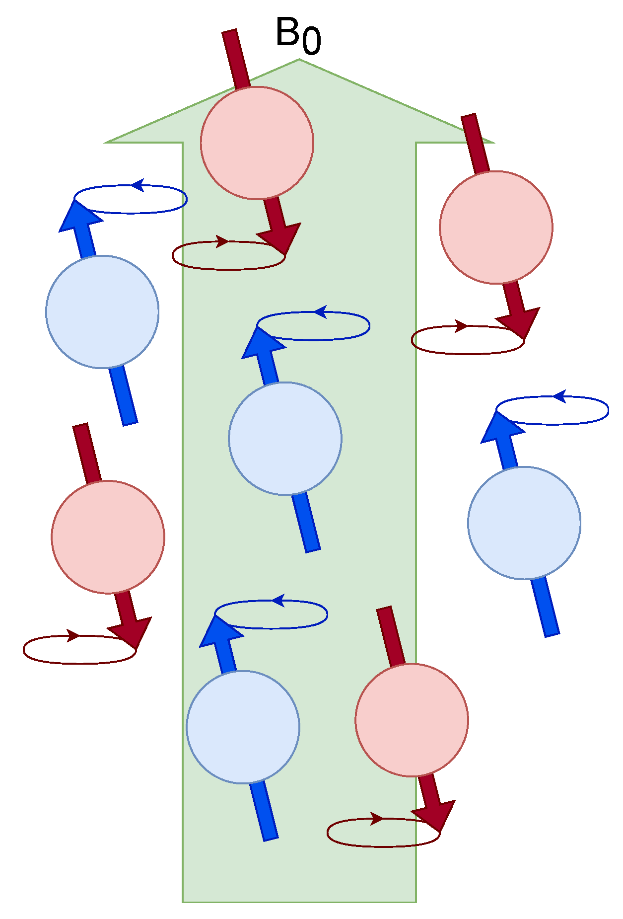
Figure 2.
Zeeman energy levels and determine the magnetization parallel to the external magnetic field given by a net value of populations aligned with that magnetic field. Radiofrequency (RF) pulse perturb the nuclear spins from their equilibrium state, which are "on resonance".
Figure 2.
Zeeman energy levels and determine the magnetization parallel to the external magnetic field given by a net value of populations aligned with that magnetic field. Radiofrequency (RF) pulse perturb the nuclear spins from their equilibrium state, which are "on resonance".
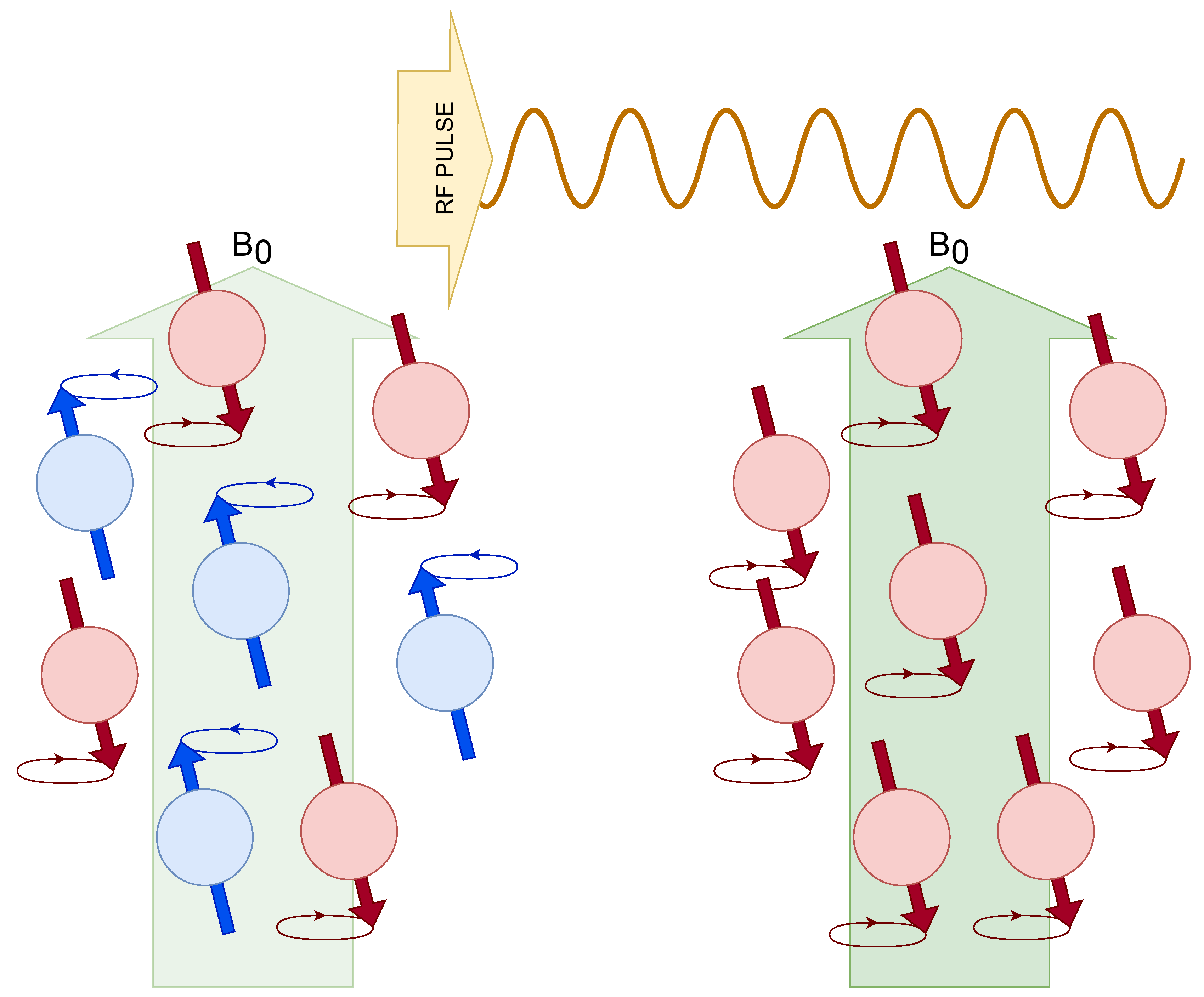
Figure 3.
Block diagram of the electrotechnical device for nuclear spin excitation in the earth magnetic field. Bp and Be represent the polarization magnetic field and the earth magnetic field respectively.
Figure 3.
Block diagram of the electrotechnical device for nuclear spin excitation in the earth magnetic field. Bp and Be represent the polarization magnetic field and the earth magnetic field respectively.
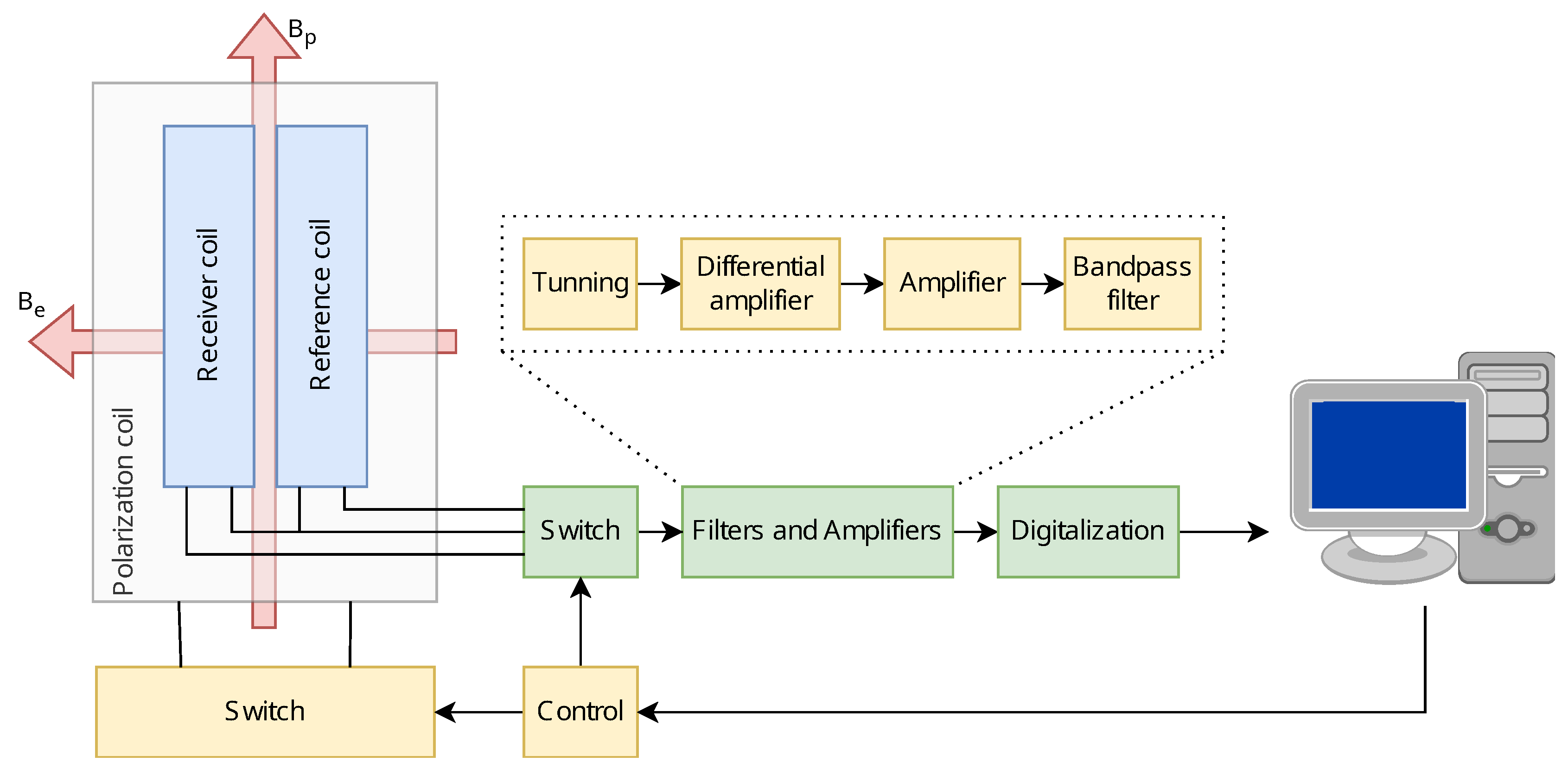
Figure 4.
CAD design of the polarizing and receiving coil cylinders.
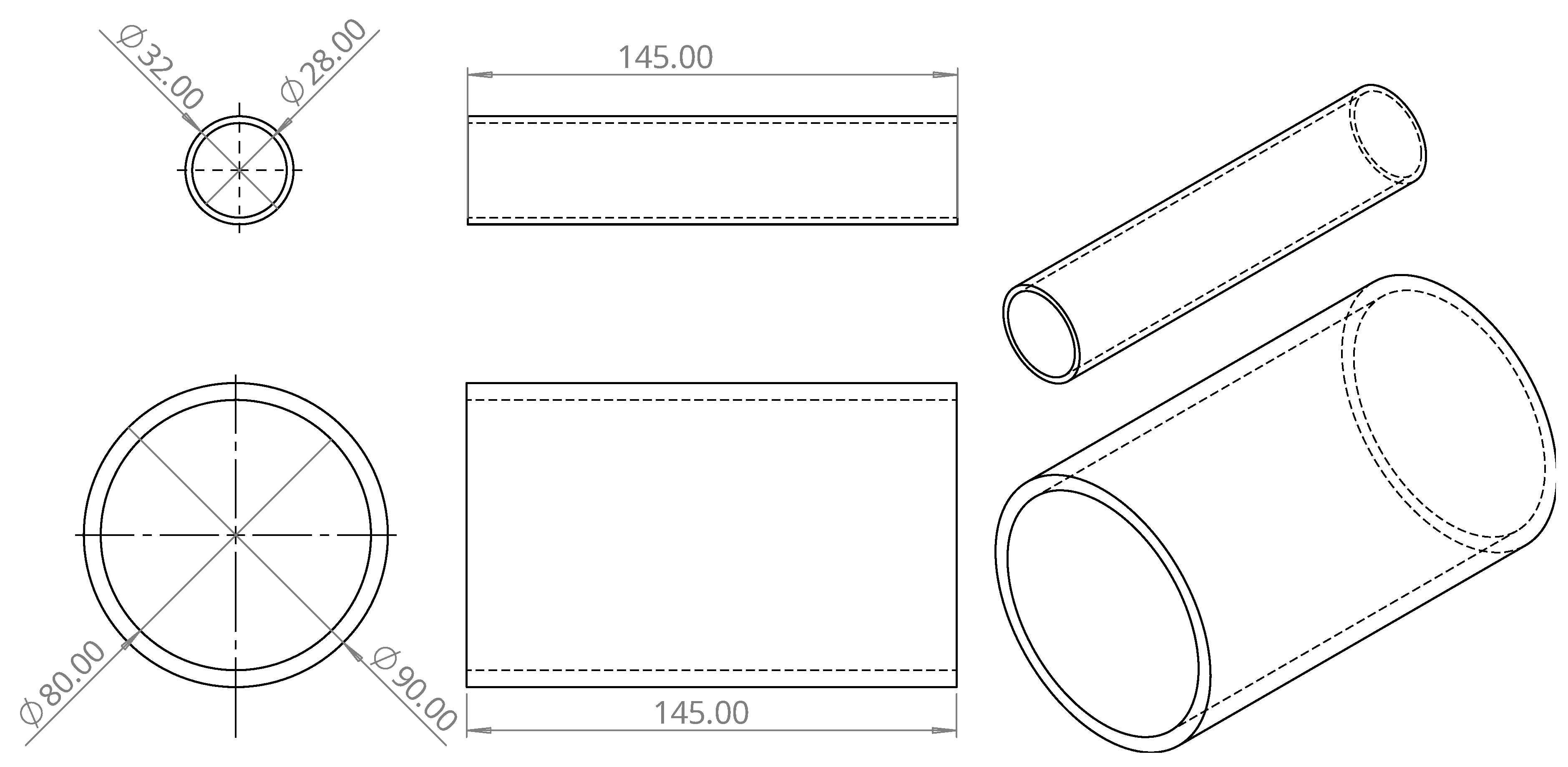
Figure 5.
CAD design of the bases that support the coils and assembled model.
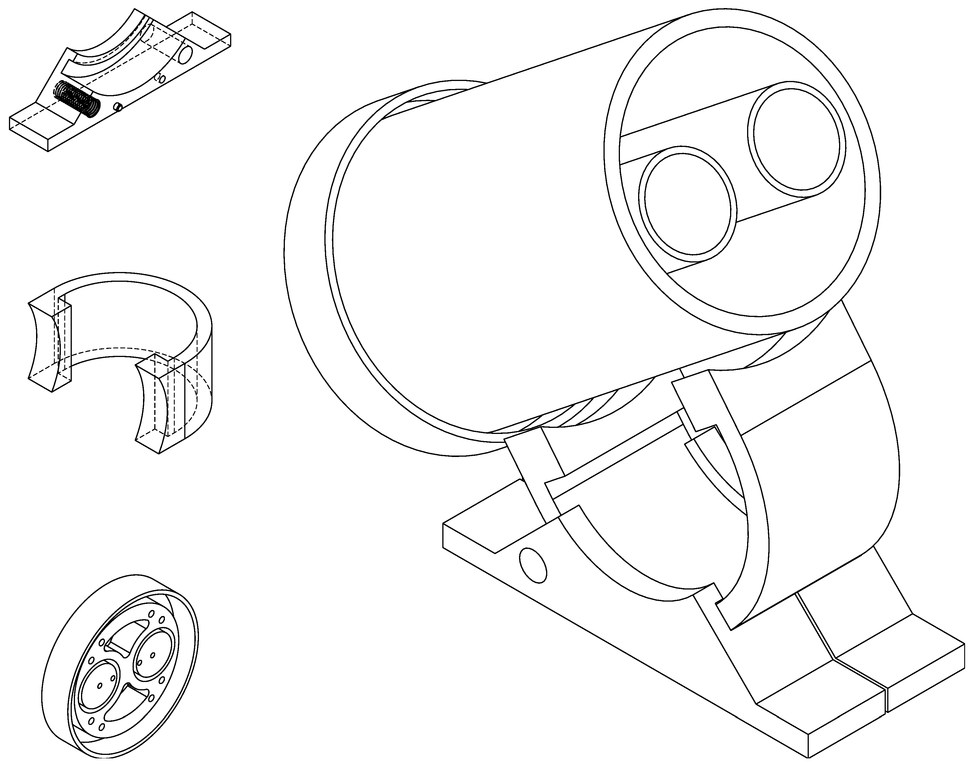
Figure 6.
3D printed parts with PETG and Nylon M10 threads
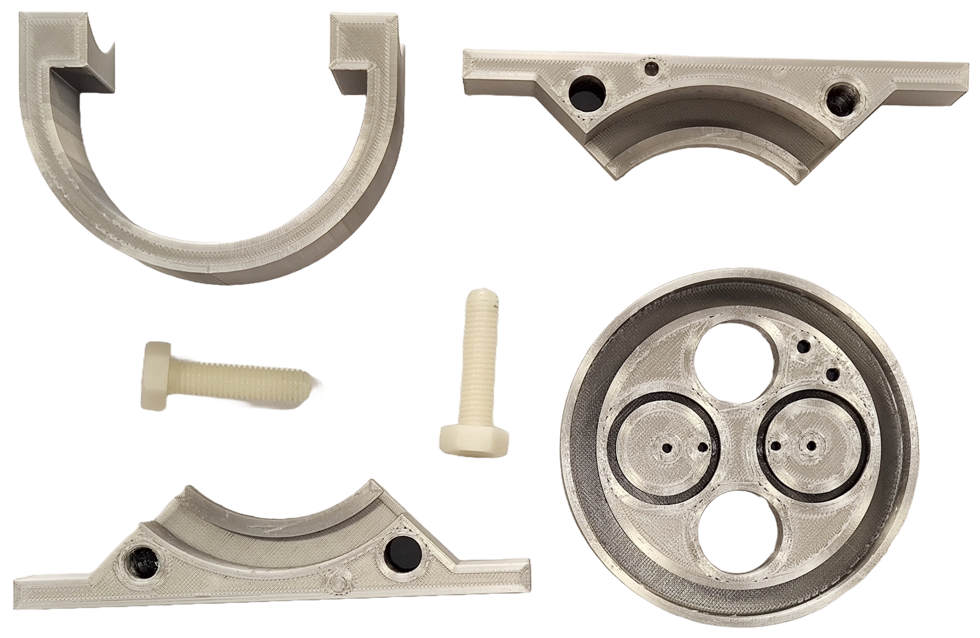
Figure 8.
Winding diagram of the receiver coils.
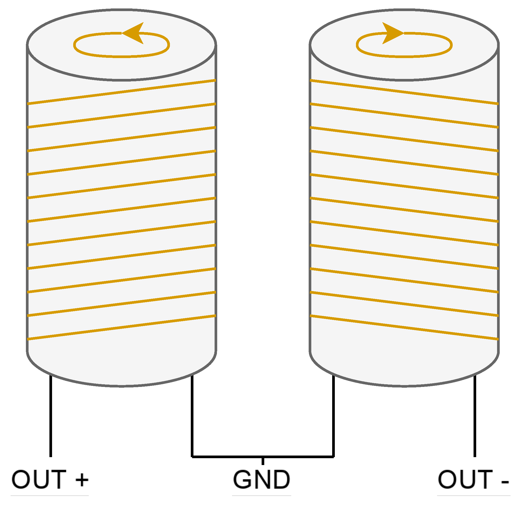
Figure 9.
Wounded receiver coil and test tube.

Figure 10.
Testing of receiver coils in the electrotechnical laboratory .
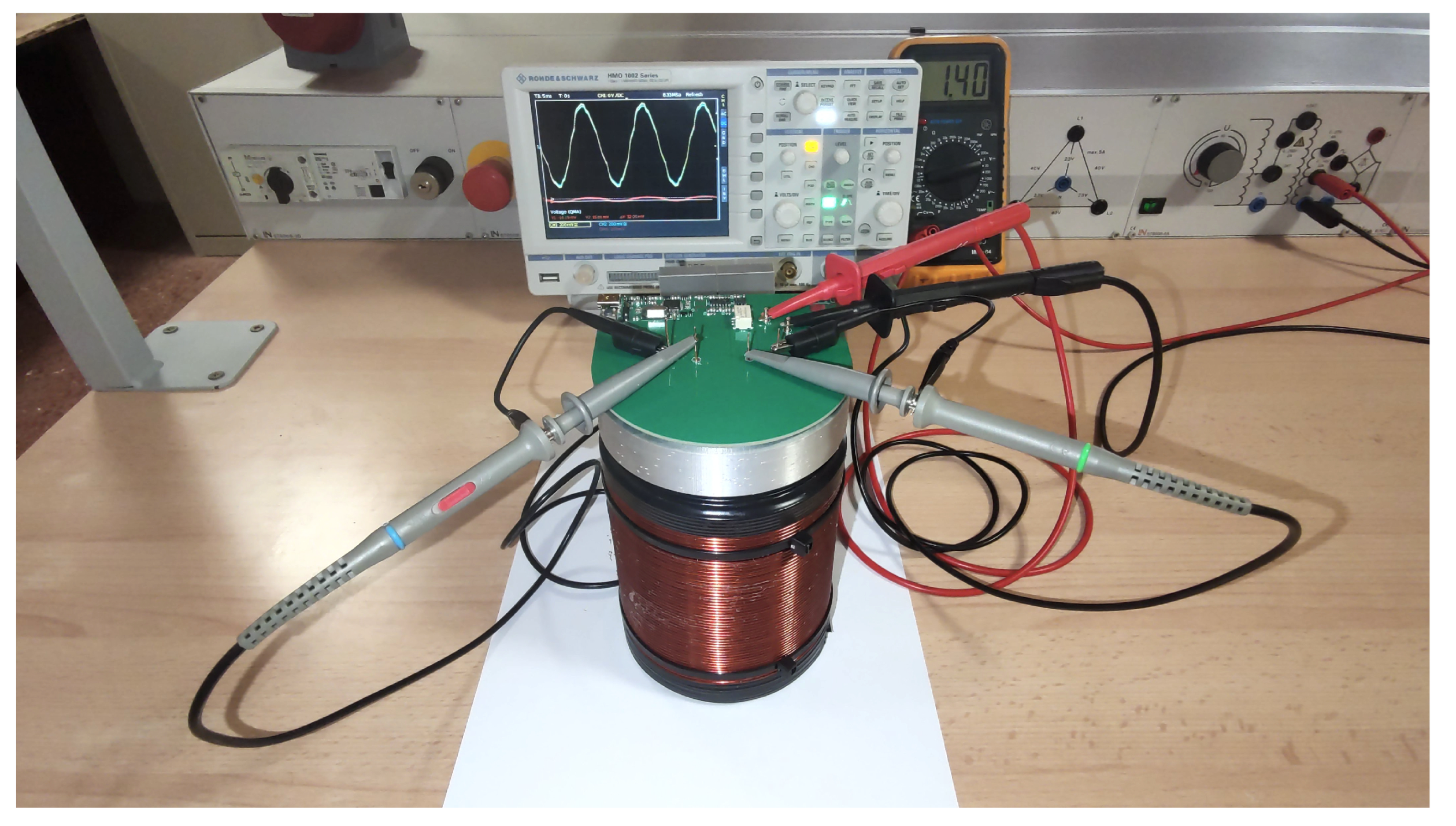
Figure 11.
Test results give a good response of the avoiding signal between both coils. Only a litle 180º dephased signal was measured which ensures the cancelation of the signals.
Figure 11.
Test results give a good response of the avoiding signal between both coils. Only a litle 180º dephased signal was measured which ensures the cancelation of the signals.
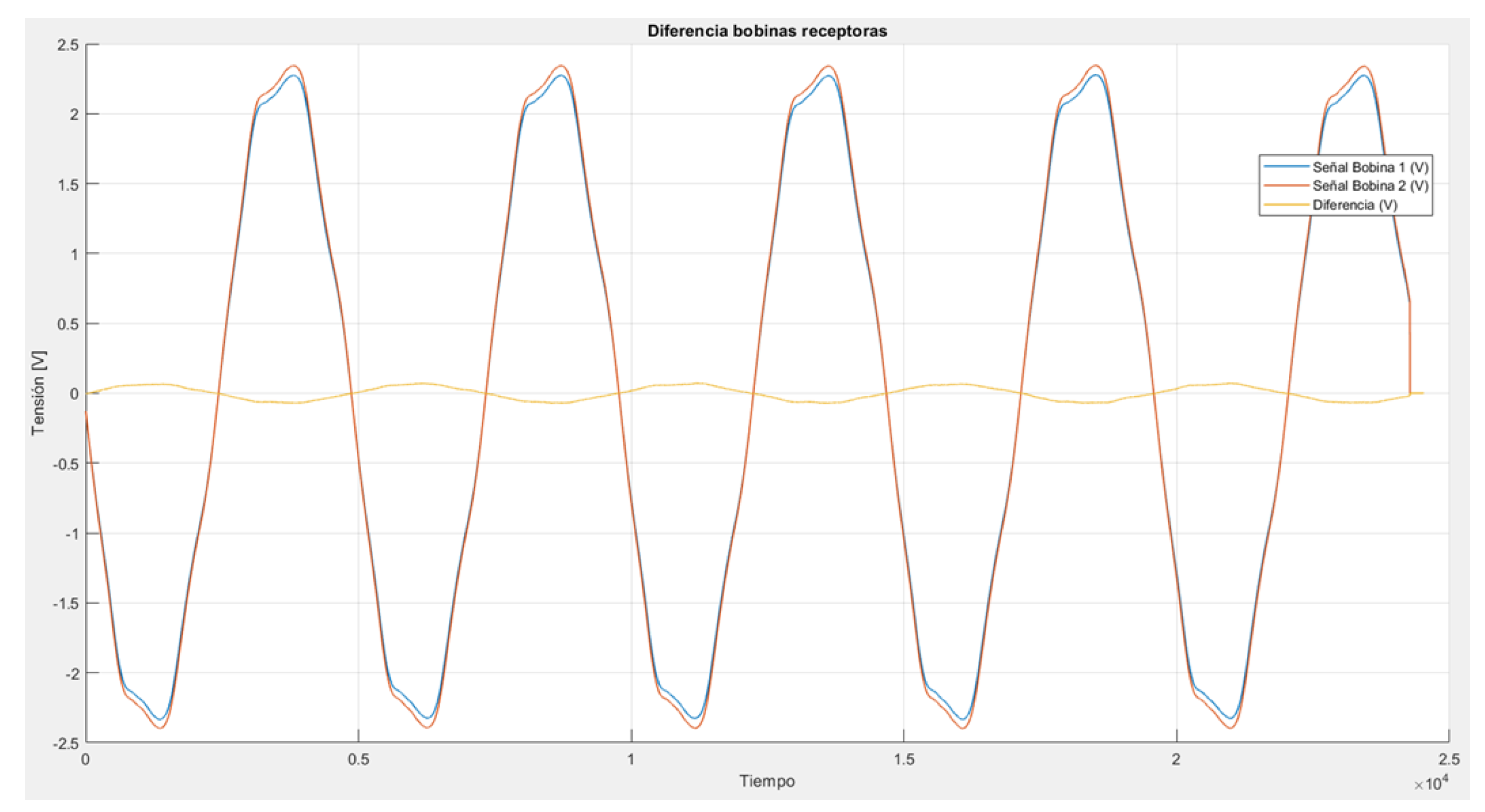
Figure 12.
Circuit schematic of excitation coil control.

Figure 13.
Block diagram of the amplification and filtering circuit.
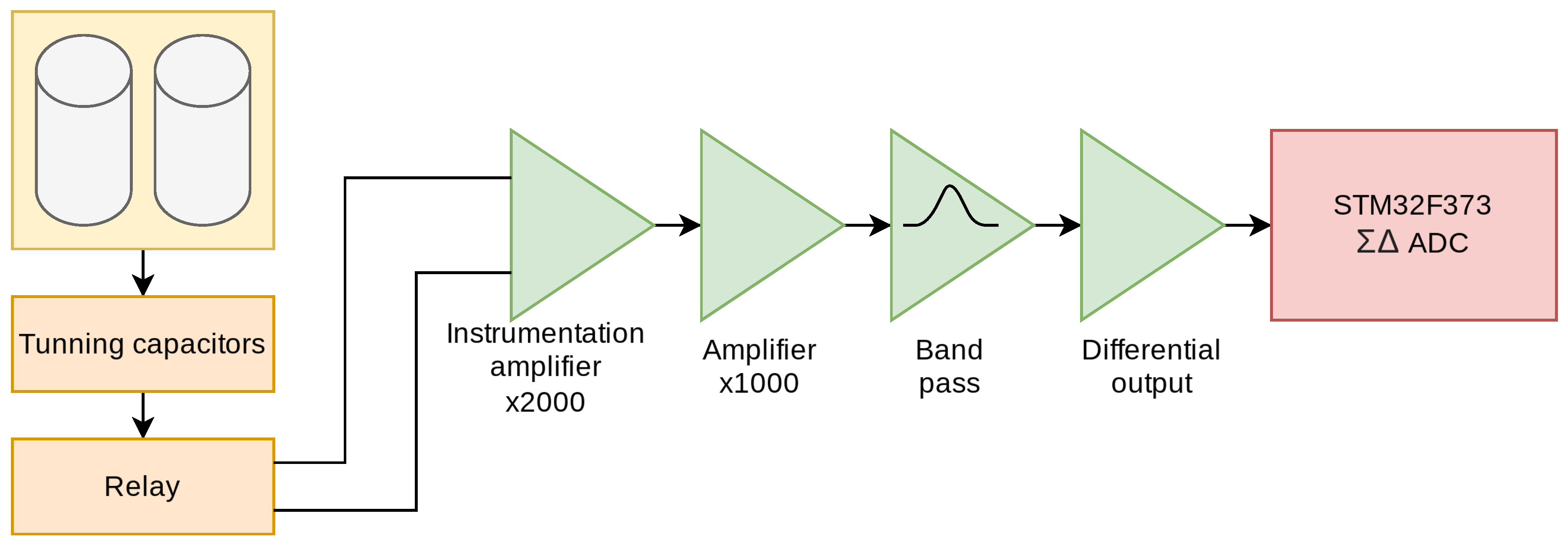
Figure 14.
Switching amplification and filtering input stages circuit.
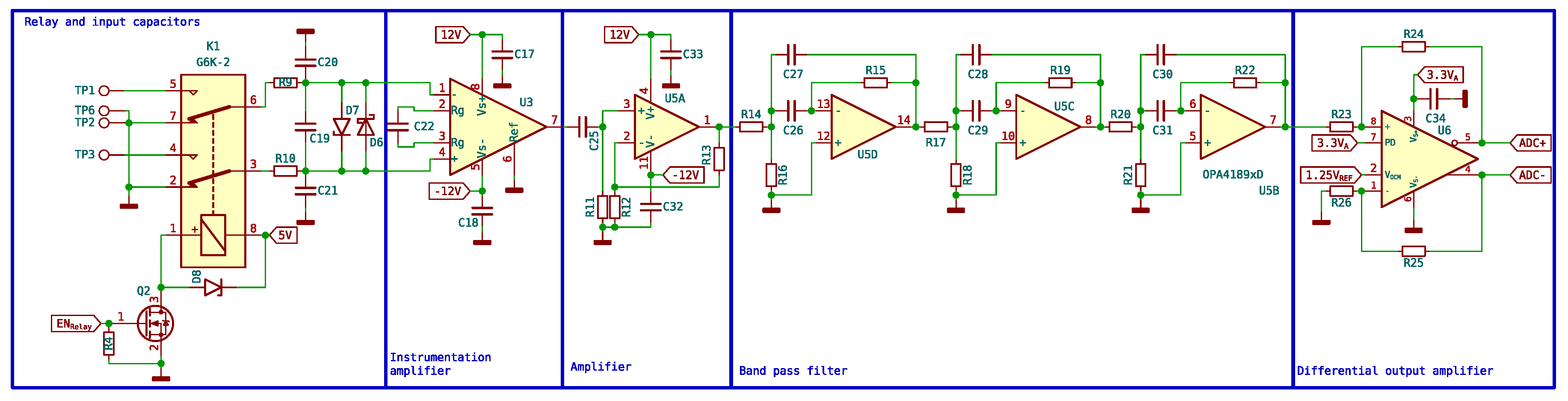
Figure 15.
Filter stage frequency response. Blue band includes components tolerances.
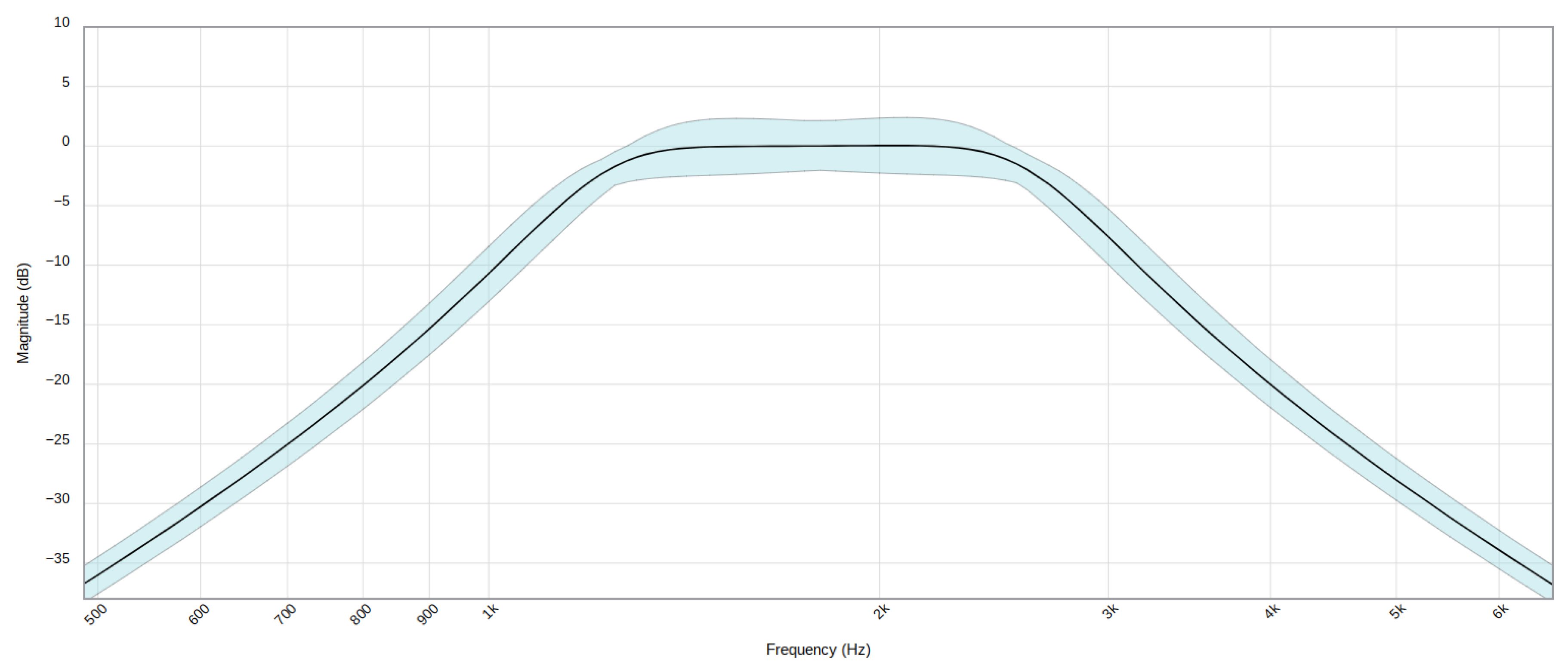
Figure 16.
Sequence of pulses followed by the device as a function of time.
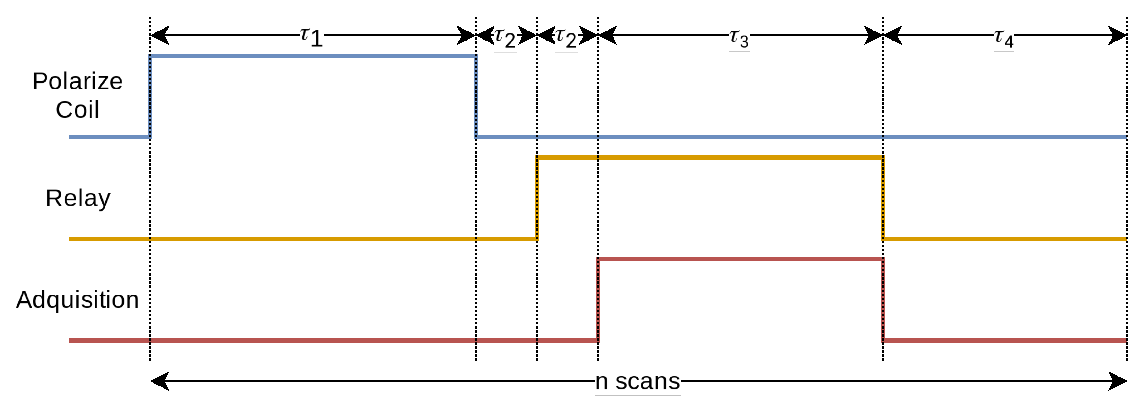
Figure 17.
Microcontroller schematic and auxiliary components.
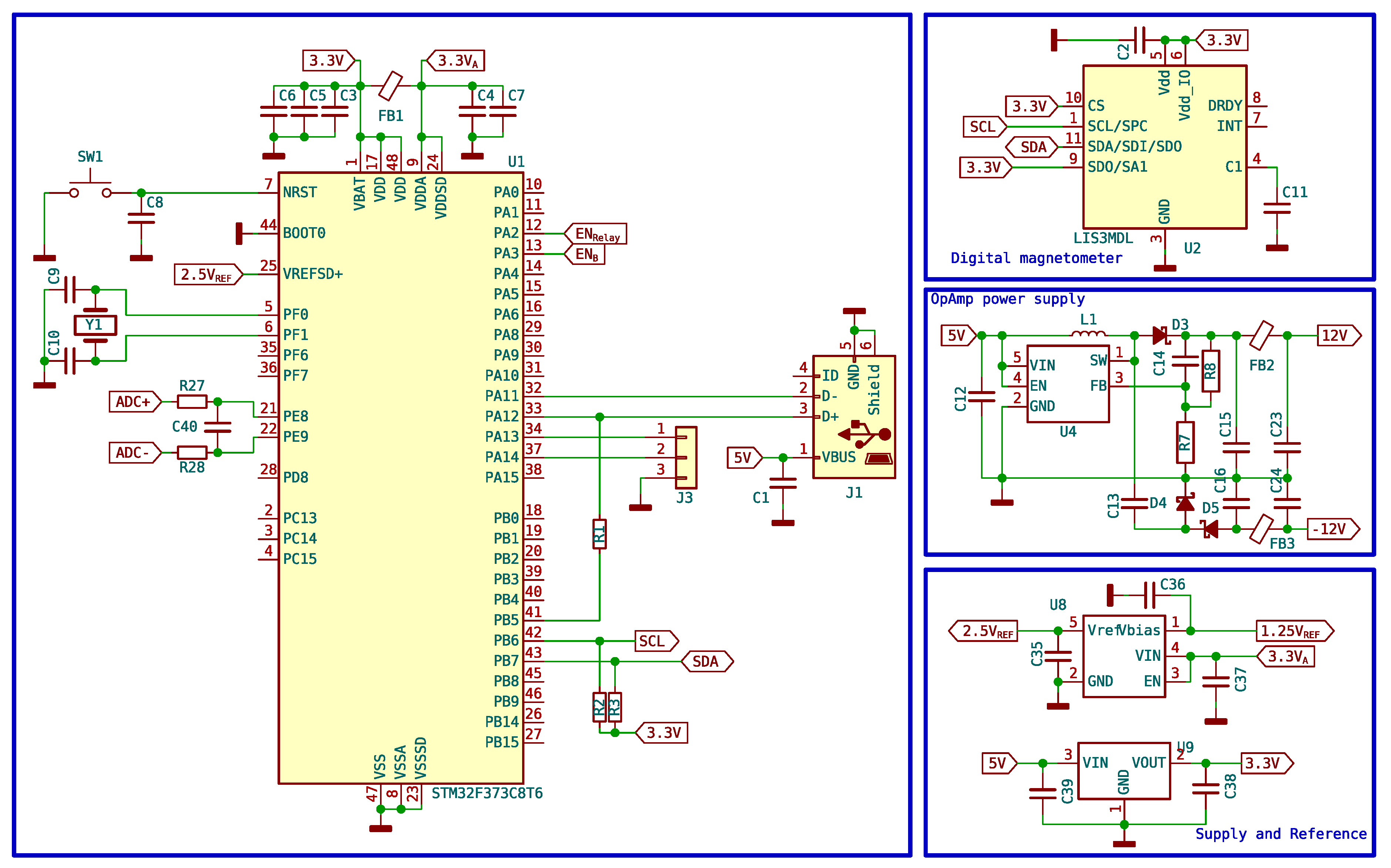
Figure 18.
The main window of the computer software is divided into two parts. On the left side, there is a control panel with textboxes and buttons for managing the acquisition process. On the right side, there is a primary plot window that displays either the detected signal or its Fast Fourier Transform (FFT) analysis.
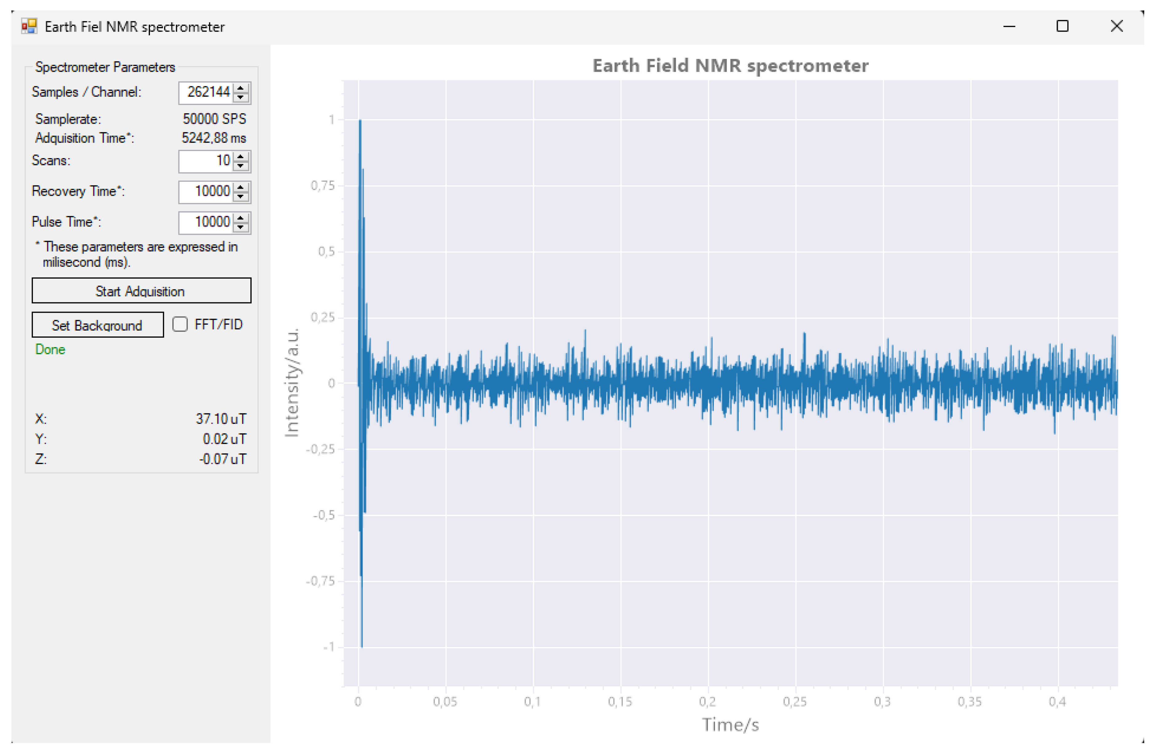
Figure 19.
The final device was successfully assembled, integrating all components into a cohesive and fully functional EFNMR spectrometer.
Figure 19.
The final device was successfully assembled, integrating all components into a cohesive and fully functional EFNMR spectrometer.
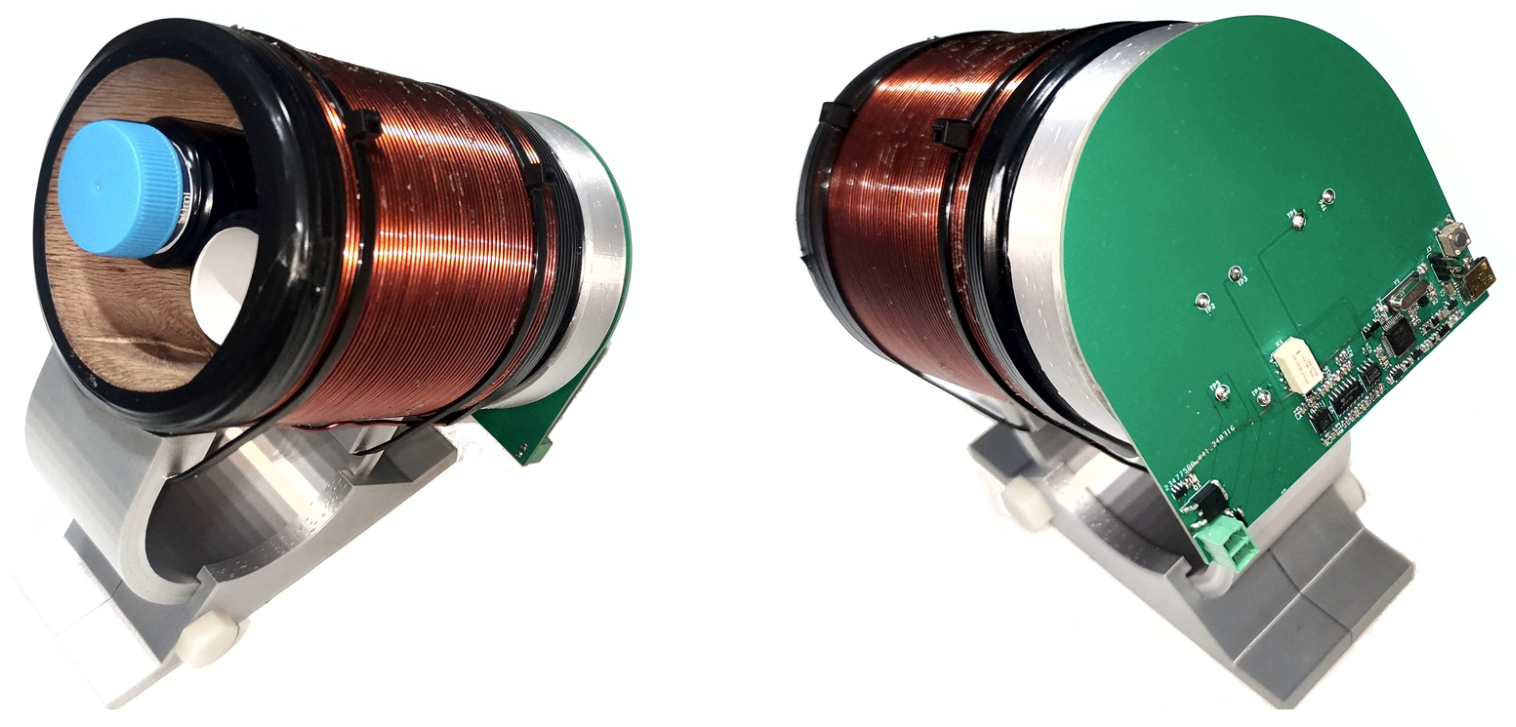
Figure 20.
1H MR spectrum test was successfully conducted. The magnetometer detected a magnetic field strength of 37.10 nT, resulting in a resonance frequency of 1579 Hz for the 1H nuclei.
Figure 20.
1H MR spectrum test was successfully conducted. The magnetometer detected a magnetic field strength of 37.10 nT, resulting in a resonance frequency of 1579 Hz for the 1H nuclei.
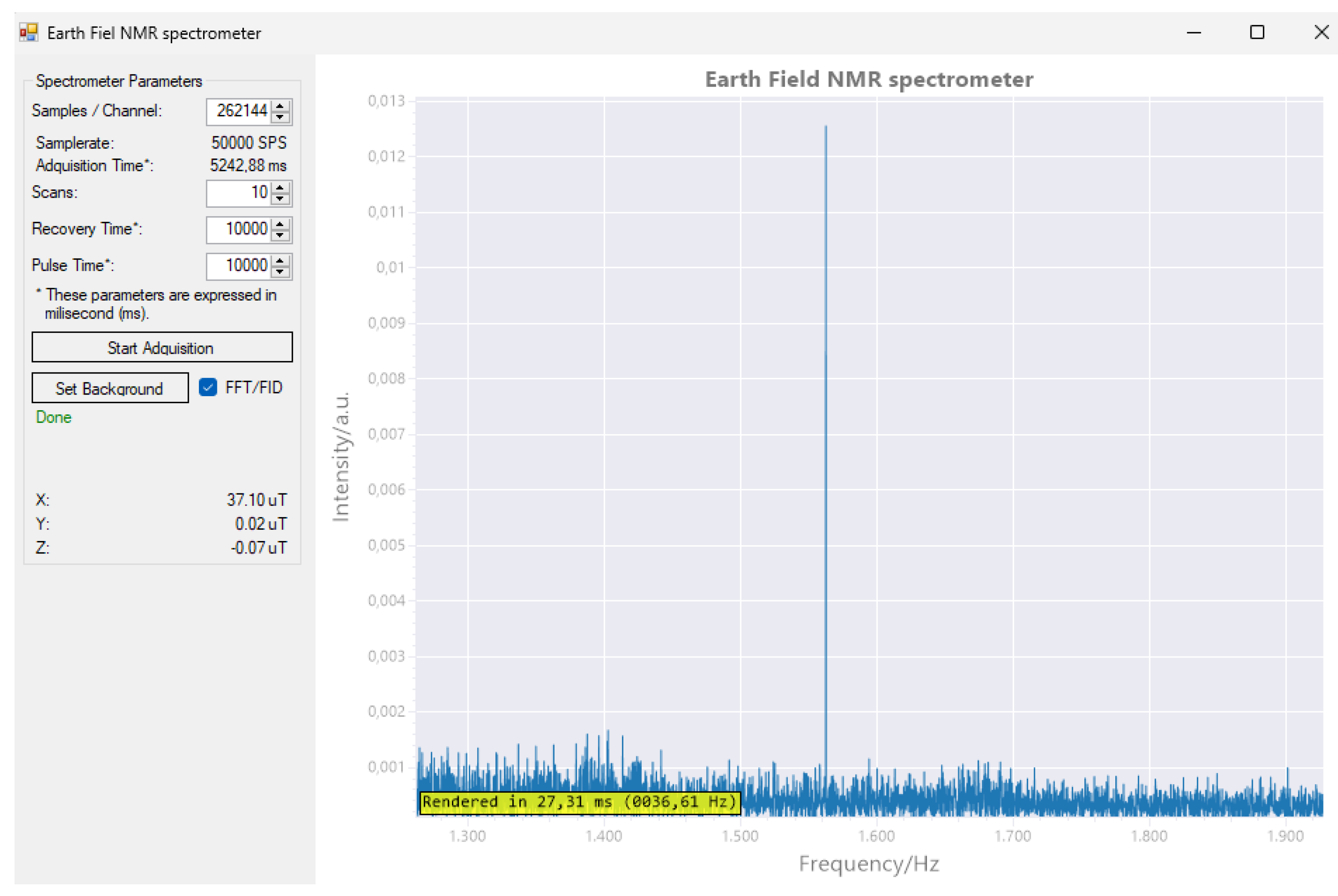

Table 1.
Model of Equilibrium and Non-Equilibrium in the Resonant Process of Nuclear Spin.
| Equilibrium | Non-Equilibrium |
|---|---|
Table 2.
Specifications of the Polarizing Coil.
| Coil | Specification |
|---|---|
| Enamelled copper wire | 1.7 mm or 14 AWG |
| Inner diameter of the coil | 80 mm |
| Outer diameter of the coil | 90 mm |
| Height of the coil | 145 mm |
| Number of wire layers | 3 |
| Number of turns per layer | 60 |
| Approximate inductance | 3.4 mH |
| Approximate resistance | 0.8 |
Table 3.
Specifications of the Polarizing Coil.
| Coil | Specification |
|---|---|
| Enamelled copper wire | 0.812 mm or 21 AWG |
| Inner diameter of the coil | 25 mm |
| Outer diameter of the coil | 40 mm |
| Height of the coil | 100 mm |
| Number of wire layers | 4 |
| Number of turns per layer | 115 |
| Approximate inductance per coil | 2.56 mH |
| Approximate resistance per coil | 2.5 |
Table 4.
Times for each stage of the sequence.
| Stage | Symbol | Minimum | Maximum | Default |
|---|---|---|---|---|
| Polarizing coil activated | 1s | 32s | 10s | |
| Pre-acquisition | - | - | 100ms | |
| Acquisition | 1000 samples | 5000000 samples | 250000 samples | |
| Adquisition samplerate | - | - | - | 50000 SPS |
| Waiting between experiments | 1s | 32s | 5s | |
| Number of scans | N | 1 | 5000 | 650 |
Disclaimer/Publisher’s Note: The statements, opinions and data contained in all publications are solely those of the individual author(s) and contributor(s) and not of MDPI and/or the editor(s). MDPI and/or the editor(s) disclaim responsibility for any injury to people or property resulting from any ideas, methods, instructions or products referred to in the content. |
© 2024 by the authors. Licensee MDPI, Basel, Switzerland. This article is an open access article distributed under the terms and conditions of the Creative Commons Attribution (CC BY) license (http://creativecommons.org/licenses/by/4.0/).
Copyright: This open access article is published under a Creative Commons CC BY 4.0 license, which permit the free download, distribution, and reuse, provided that the author and preprint are cited in any reuse.


