Submitted:
19 July 2024
Posted:
20 July 2024
You are already at the latest version
Abstract
Acousto-Optical Tunable Filters (AOTFs) are a promising technology, exceptionally suited for advanced applications in spectroscopy and imaging across various scientific fields, including space exploration. This is due to their flexibility and high-speed functionality for precise wavelength selection via periodic modulation of the crystal’s refractive index using sound waves. These AOTFs are in turn driven by Radio Frequency (RF) signals through a transducer creating sound waves inside the crystal. This work presents a detailed comparison of three distinct topologies of Radio Frequency Power Amplifiers (RFPAs) for driving these AOTFs within the 30 to 300 MHz frequency range. The analysis focuses on three critical parameters: efficiency, bandwidth, and linearity, which are essential for optimizing the performance of AOTFs. By evaluating the trade-offs among these parameters, this research aims to identify the most effective design approach for RFPAs in this application context.
Keywords:
AOTF
; RFPA
; Class E
; efficiency
; harmonics suppression
; linearity
1. Introduction
The measurement of the atmosphere is crucial for understanding its complex behavior and its implications across several scientific disciplines, including meteorology, climatology, atmospheric chemistry, and environmental studies [1,2]. Due to its intricate nature, the study and measurement of the atmosphere requires sophisticated tools and methods to ensure precise observation and analysis of its characteristics.
In this context, the Acousto-Optical Tunable Filter (AOTF) emerges as an innovative technology based on the interaction between sound and electromagnetic waves [3]. The AOTF operates by an applying a pure Radio Frequency (RF) sinewave to a transducer mounted to a crystal that induces acoustic waves inside the crystal as shown in Figure 1. A piezoelectric element is responsible for the generation of these sound waves. These acoustic waves in turn cause a periodic modulation in the crystal's refractive index, enabling the precise and selective filtering of light across specific wavelengths [4]. Depending on the frequency and power, different optical wavelengths can be selected [5]. The incoming light must enter the AOTF at a specific angle known as the Bragg Angle, . By precisely aligning the light with this angle, the acoustic wave interacts optimally with the light, resulting in effective modulation and selective transmission of desired wavelengths [6]. The adaptability and tunability of the AOTF make it an excellent choice for applications in spectroscopy and imaging, where it can filter and manipulate light effectively making it perfectly suited for space applications [7].
The fundamental building blocks necessary for driving these AOTFs consist of i) a RF generator along with ii) a Radio Frequency Power Amplifier (RFPA) as shown in Figure 2. RFPAs are the most power hungry components in this AOTF chain. They are a notable source of power dissipation and non-linearity. Additionally, the heat generated[8] during operation can potentially compromise the precision of measurements in scientific instruments that rely on optics [9,10,11].
The RFPA plays an important role in ensuring the efficiency and optimal performance of the AOTF system. These amplifiers are assigned with the critical task of boosting the RF signal to the desired power level without any distortion. One of the key factors for these amplifiers is maintaining high efficiency and minimizing heat dissipation, thereby preventing adverse effects on the sensitive optical setup. AOTFs are sensitive to temperature variations, and excess heat could lead to degradation in performance or even damage [12]. The RF signal for driving AOTFs typically falls in the VHF (30-300 MHz) band with an optimal driving power ranging from 100 mW to 3 Watts with the harmonics suppressed below -30dBc [13].
Addressing this power efficiency, advanced semiconductor materials like Gallium Nitride (GaN) or Silicon Carbide (SiC) have already been explored in the RFPA design [14]. Additionally, adopting linearization techniques [15], and implementing effective cooling solutions [16] are also the integral aspects of RFPA design. For space based systems there is a huge limitation on reliable semiconductor technologies that can be used along with the limitations to use complex linearization or cooling techniques [17]. Hence, simple and efficient design topologies have to be used.
Designing a highly efficient RFPA is essential to meet these challenges, ensuring precise wavelength tuning and selection, while adhering to stringent power and thermal constraints in space environments[18]. Typically, the design of an RFPA starts with the selection of its class. Traditionally, an RFPA is based on standard biasing conditions (Class A, AB) or operating conditions (Class E, F) [19]. To achieve an highly efficient RFPA, the power lost at the device must be minimized by imposing the non-overlapping condition given by Equation 1.
This non-overlapping condition makes the theoretical efficiency of the Class E and Class F amplifiers 100%. The time domain voltage and current waveforms for the RFPA illustrated in the Figure 3. However, to achieve the square waveform in class F, the use of multiple resonators is necessary [20] thereby making the use of Class E as one of the promising solutions.
The historical evolution of Class E RFPAs dates back to the late 1940s [21]. In the late 1960s switched mode power amplifiers became popular due to the inherent non-overlapping condition. Equation 1, which can be further expanded into the Zero Voltage Switching (ZVS) and Zero Voltage Derivative Switching (ZDS) given by Equation 2 and 3 [22] . However, it was in 1975 that Sokal et. al [23] introduced the term Class E for the first time, while the explicit design equations were provided by Raab in 1977 [24].
In similar context there has been two common load network topologies for Class E RFPAs, one where the effect of finite DC feed is ignored [25] and another considering these effects of finite DC feed [26]. Nevertheless, both configurations incorporate a series resonator to force the fundamental current into the circuitry. With the emerging field of wireless technologies, transmission line based Class E RFPA topology was explored in [27,28]. However, for the design of RFPAs in the VHF range, the use of transmission line becomes impractical and the use of discrete/lumped R L C components becomes inevitable.
In general the design on the load network [29,30] poses a significant challenge for the study of wideband class E RFPAs. Previous work extensively describes various effects on the load network but leaves a gap regarding the frequency-dependent characteristics of these design equations [31]. Moreover, it lacks a comparison of design topologies to achieve the best trade-off in efficiency, bandwidth, and linearity, without the use of any additional filters or complex circuitry at the output. This is important so that the RFPA can be easily implemented within the framework of space-based applications.
This work starts with the descriptions of the fundamentals of Class E RFPAs considering the finite feed DC as well as infinite DC feed in Section 2. It then presents the key design parameter, i.e. the Quality Factor (Q), and its trade-offs in Section 3. Finally, by incorporating an additional resonant tank circuit, a design methodology is provided to achieve the best possible trade-off among the three factors in Section 4. This approach eliminates unnecessary circuit optimization, which is time-consuming and often fails to converge. Finally, the paper concludes with the results and discussion in Section 5 and 6. The simulations conducted in this work are verified through harmonic balance (HB) simulations, using the 10 Watt CGH40010 transistor [32], having space heritage [33,34].
2. Theoretical Analysis
This section delves into the basic design equations of a Class E RFPA along a study on the efficiency and linearity which varies with frequency. For simplicity, the switching duty cycle is considered to be 50 %, with the zero on resistance. Based on the literature two highly used topologies are described [35]: 1) the finite DC feed, and 2) the infinite DC feed. These configurations affect the performance and efficiency of the amplifier.
- Class E with infinite DC Feed: is a more idealized model where the DC feed inductance is assumed to be infinite. In practice, this means that the inductance is large compared to other reactance’s in the circuit. This configuration simplifies the theoretical analysis of the amplifier and can lead to idealized performance predictions, such as very high efficiency. However, in practical applications, achieving truly 'infinite' inductance is impossible, so this model serves more as a theoretical benchmark or a design starting point.
- b. Class E with finite DC Feed: here the DC feed inductance is finite, meaning it has a specific, non-infinite value. This configuration is more practical and commonly used in real-world applications. The finite DC feed provides a certain level of control over the amplifier's operation, including aspects like the RF waveform shape and the amplifier's efficiency. However, the finite value of the inductance can introduce additional considerations in the design, such as the impact on bandwidth and stability.
Both configurations aim to optimize the performance of Class E amplifiers, particularly in terms of efficiency and power handling. The choice between a finite and an infinite DC feed depends on the specific requirements of the application, such as the desired efficiency, frequency range, power level, and practical considerations in circuit design and implementation. A detailed comparison of these design approaches is presented in this work to generate a tradeoff, specifically for VHF band.
2.1. Class E Load Network Topology with Infinite DC Feed
The fundamental circuit configuration of a Class E tuned switched-mode power amplifier with a parallel circuit is illustrated in Figure 4(a). This configuration is referred to as Topology 1 in this work without the loss of generality. The load network encompasses a parallel capacitance (C = Cdev + Cext ) that represents the device inherent capacitance, Cdev along with any external capacitance, Cext which ensures the current in and out of the switch-capacitor combination. A additional series inductance L that produces a reactance, jX with a series resonant circuit (Ls-Cs) tuned at the fundamental frequency, fo, is then finally connected to the optimal load resistance (R). The supply voltage is Vdd and Vbb the biasing voltage with an RF Choke. is and vs are the voltage and current in the ideal switch respectively. iC , I0 and iR are the currents flowing through the capacitor C, RF choke, and load R. The equivalent circuit is shown in Figure 4(b). The load current flowing through the load is given by,
in which, ϕ is the initial phase shift and IR is the current peak amplitude.
When the switch is on with the initial on state condition, the DC current can be defined as I0 = -IR sin(ϕ) and the switch current can be written as,
With the switch being off, the current through the capacitor can be written as,
and the switch voltage is given by,
The primary objective of the problem is to find the unknown parameter, IR and ϕ. With the ZVS given by Equation 2, the value of the initial phase shift is ϕ = 57.5180 and IR,max = 2.8621I0 . Using the Fourier series [36], the load impedance can written as,
The values of C and L then is given by,
and the optimal load resistance is given by,
2.2. Class E Load Network Topology with Finite DC Feed
Since realizing infinite DC feed in all topologies is problematic, a new topology is proposed in which the finite DC feed is replaced by the finite value of L.
The configuration of a Class E tuned switched-mode power amplifier with a finite DC feed is illustrated in Figure 5(a). The load network encompasses a feed inductance (L) with the additional series reactance, jX connected to the series resonant circuit (Ls-Cs) tuned at the fundamental frequency fo. The equivalent circuit along with the direction for the given circuit configuration is shown in Figure 5(b). The load current is given by,
where, ϕ is the initial phase shift and IR is the current peak amplitude. For the time interval, , the switch is on and the current flowing through the switch can be given by (applying the initial condition) as,
When the switch is off in the interval , the current through the switch becomes zero and the current in the capacitor can be given by , with the initial condition for the feed inductance L,
The switch voltage can be found by solving the differential equation as reported in [35]
Without the loss of generality, and using the initial off state conditions, we have
With variable q as a free parameter, the values for the unknow parameters, and p can be calculated, using the ZVS and ZVDS conditions. Two equations with two unknowns can be solved using Equation 25 and 26 to get the required values,
The parameter q, imposes limitations owing to the extensive design space and complex design equations. A comprehensive tutorial addressing these considerations has been reported by Casallas et al [37]. This is simplified in this work by evaluating two extreme scenarios: when jX = Lx (q = 0.5) and when jX = 0 (q = 1.412).
With q = 0.5, the above equations (25) and (26) can be solved to get the value of p = 21.3 and This configuration is referred as Topology 2.1 in this work without the loss of generality. Finally the closed form expressions for R, L C and Lx can be calculated as follows,
Similarly with q = 1.412 we have p = 1.210 and . This configuration is referred as Topology 2.2 in this work without the loss of generality. The values for R, L and C can be calculated as follows,
3. Quality Factor (Q) and It’s Trade-Offs
To further investigate the effect of the quality factor (Q) of the series resonator and its effect on efficiency bandwidth tradeoff, a 1 Watt amplifier is simulated using CGH40010 at 50 MHz, supply voltage of Vdd = 10 V, biased at Vbb = -2.45 V. With an output power of 1 watt the load network parameters are calculated for all the three topologies, as indicated in Table 1.
With Q being the quality factor of the series tank circuit, Ls and Cs the values of the filter, which are given by,
And the values listed in Table 1, harmonic balance simulations are performed by varying Q. The Power Added Efficiency (PAE) and the output power till 3rd order for all the three topologies are listed in the Table 2.
Based on the above simulation, the dependance on the efficiency bandwidth product with the sacrifice in linearity is inevitable in all the topologies. Efficiency versus frequency is depicted in Figure 6 for the three topologies. For Topology 1 and 2.1, the efficiency versus frequency graph follows a similar trend. However, for Topology 2.2, the behavior of the graph as a function of the Q factor is completely different. This difference could be explained by studying the load network separately which is discussed in the preceding part.
Based on the simulations, the bandwidth can be enhanced by lowering the Q factor of the series filter . However, this adjustment results in a significant increase in harmonic levels, necessitating the use of an additional filter. This additional filter, in turn, further degrades the overall efficiency of the RFPA. Therefore, a tradeoff is necessary between these three factors limiting the design options.
To further explore the different topologies, the load network is examined in detail. The relationship between phase and frequency for the load network at various Q values is illustrated in Figure 7. For Topologies 1 and 2.1, the phase versus frequency behavior changes sharply as the Q values increase. However, the 2.2 topology exhibits a distinct pattern in its efficiency-bandwidth graph compared to the first two topologies. Specifically, for a particular value of Qopt, the phase angle vs frequency is exactly the same as obtained through the reactance compensation technique [39].
It is also evident from the data that there is a nearly perfect correlation between the phase angle versus frequency graph and the efficiency graphs. This correlation underscores the critical role of the load network in maintaining optimal Class E operating conditions.
Mathematically, the input impedance for the topology 2.2 can be written as Equation 36. On applying the reactance compensation technique, Equation 36 can be equated to zero to find the value of L0.
The values of the series resonator Ls and Cs becomes Lo and Co and is given by Equation 37 and 38,
Using the value of L0 from Equation 37 in Equation 35, the optimal value of Q can be given as,
This analysis demonstrates that while an improvement in the efficiency-frequency response was attained, it comes at the cost of the RFPA’s linearity. Hence, the wideband response introduced by Topology 2.2 led to inadequate suppression of harmonics, constraining the overall design strategy. Despite these limitations, this approach represents the optimal scenario for achieving a relatively flat load angle response compared to Topology 1 and 2.1, thereby optimizing the efficiency and bandwidth. However, achieving a balance among efficiency, bandwidth, and linearity requires the incorporation of extra circuitry which is explored in the subsequent section.
4. Design Methodology : Importance of Harmonic Termination
In all described cases, it has been observed that although the Q factor is an effective mean to enhance the system's bandwidth, there are limited options for further tuning to address the 2nd or 3rd harmonic. Consequently, this situation necessitates the introduction of additional circuitry, all while adhering to the Class E design parameters.
Let us now consider the circuit shown in Figure 8. The equivalent impedance is given by Equation 40. The resonator is represented by L2 - C2 which is resonant at the 2nd harmonic making it an open circuit, while the 3rd is shorted.
In order to maintain the ideal Class E condition, the total impedance must be equal to the = . Applying the 2nd and 3rd harmonic condition given by and in Equation 40, the circuit values can be found as,
Here LE represents the impedance that needs to be mapped.
However it is seen that the circuitry controls the 2nd harmonic performance while the third harmonic level is still high, thereby degrading the performances. Hence, to further facilitate the design a 3rd harmonic resonant tank circuit is added to the output. The vales of the C3 –L3 with Q3 representing the quality factor of the 3rd harmonic resonant tank circuit is given by,
The phase angle as well as the magnitude for this modified topologies are compared to topology 2.2 at 50 MHz, as depicted in Figure 9. The graph shows that this topology with both 2nd - 3rd (referred as H23) tuning exhibits a sharper roll-off, compared to its predecessor (referred as H2). Additionally, this topology exhibits a superior impedance magnitude at the third harmonic, outperforming the previously discussed configurations in terms of performance. This advancement suggests the possibility of achieving an enhanced harmonic response alongside maintaining the optimal load condition across a broad frequency spectrum.
Harmonic Balance Class E simulations were performed in Keysight ADS to validate the non-overlapping characteristics of voltage and current waveforms in the time domain, as illustrated in Figure 10. These waveforms were further analyzed in the context of harmonic tuning, incorporating both 2nd and 3rd harmonic adjustments.The comparative analysis distinctly demonstrates a key difference when comparing with the traditional parallel Class E configuration, as identified in section 2.2. By incorporating tuning for both the 2nd and 3rd harmonics (referred to as H23), it effectively mitigates voltage and current stresses, while still preserving the non-overlapping condition specified in Equation 1.
The complete circuit of this modified topology is shown in Figure 11, in which the idealized values can be calculated using the equations in the previous sections. Given the modifications applied to the topology, an algorithm has been developed to aid the designers:
- Set the Design Frequency: Begin by specifying the frequency at which the design will operate. This is a critical first step that influences all subsequent parameters and choices.
- Determine Required Bias Voltage Levels: Identify the necessary bias voltage levels for the design. These levels are essential for ensuring the proper operation of the components within the design and the output power.
- Calculate Idealized Values: Compute the ideal values for the critical design parameters. These calculations will serve as a reference for the initial simulation and guide the optimization process.
- Run Initial Simulation: Input the idealized values obtained in step 3 into the simulation tool. The outcomes of this simulation should include suppression of the second harmonic and high efficiency at the design frequency.
-
Optimize with Fixed Capacitance Co: Keeping the capacitance constant Co, conduct an optimization over a bandwidth of 20%, aiming for 4 specific goals to get the optimum values for R, L, C, L1, L2, L3, C2 and C3 once convergence is reached. The search is done within the range of [0.5 - 2] times the values of R, L, C while [0.5 - 3] times L1, L2, L3 , C2 and C3 from the theoretical values to get the best possible design.
- -
- The fundamental frequency should achieve the required power level.
- -
- The second and third harmonics should be suppressed to X dBc.
- -
- The second and third harmonics should be suppressed to X dBc. (required level)
- -
- The PAE must be at least PP % (PP is the targeted value)
- Adjust for Different Power Levels: If there is a need to optimize for a different power level, ensure to maintain the ratio of voltage to power constant. This approach preserves the similarity in optimum resistance R values across different power levels, facilitating a scalable design strategy.
- Finalize the Design: With the optimization complete, review the design parameters to ensure they meet the desired specifications. Adjustments can be made as necessary to fine-tune the design.
Since there is a strong dependance of the external load network with the tradeoff efficiency, bandwidth and linearity, for a passive network the Bode-Fano limit [40], given by Equation 46, ensures an optimal design parameters where convergence is achieved during optimization.
Here, K is a constant and is the reflection co-efficient.
5. Results and Discussion
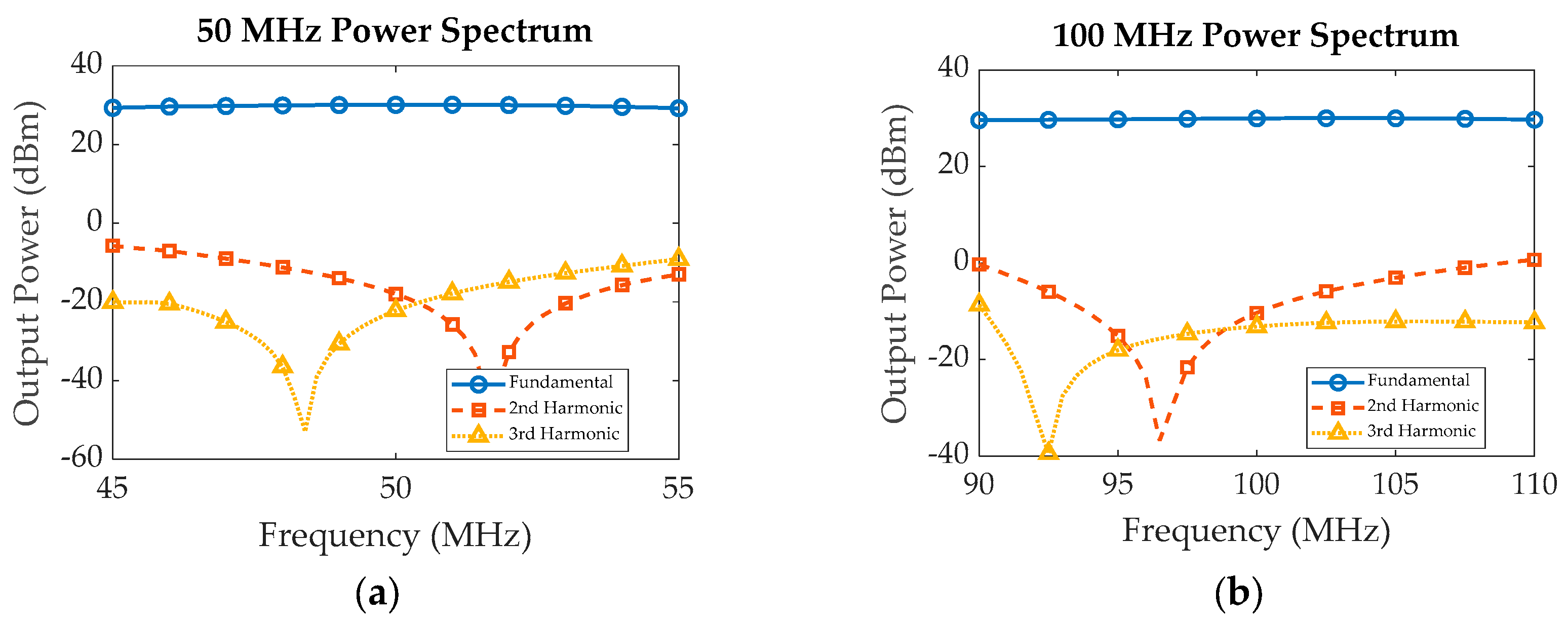
To validate the proposed methodology and demonstrate the scalability of the design approach, simulations were carried out at 50 MHz and 100 MHz for an output power of 1 Watt with a supply voltage of 10 V, utilizing the 10 Watt Wolfspeed nonlinear device model. Theoretical and optimized/practical values derived from these simulations are given in Table 3. Additionally, simulated power levels and efficiency at these two frequency designs are depicted in the corresponding Figure 12 and Figure 13.
Both configurations achieved an output power of 30 dBm, with minor fluctuations of ±1 dBm, while effectively suppressing harmonics up to the 3rd order below 30 dBc. The bandwidth achieved was around 20%, aligning with the initial guidelines set by the algorithm. While there's potential to enhance the bandwidth further, it would necessitate compromising either linearity or efficiency.
The algorithm outlined provides a systematic approach to design and optimize a power amplifier within specified parameters. The initial values generated from this algorithm facilitate the best possible trade-off among efficiency, linearity, and bandwidth for the final design.
Moreover, the optimization process converges to offer the most suitable design option among the various topologies. This is substantiated through nonlinear simulations performed using the prescribed design approach. Consequently, this method not only streamlines the design process by eliminating unnecessary optimization steps, but also ensures that the design goals are efficiently met, saving significant time and resources.
6. Conclusions and Future Work
This work examined the potential for achieving the best possible Class E topology without resorting to overly complex circuitry, focusing on efficiency-bandwidth and linearity product comparisons. The selection of the optimal topology was validated by examining the phase of the load network. It was determined that q = 1.414 (topology 2.2) is one of the best choices through detailed mathematical calculations and non-ideal simulations, as it ensures a constant load angle when the series resonator is properly tuned through reactance compensation techniques. This work also employs straightforward design equations to achieve the best possible trade-off while maintaining optimal load impedances. Utilizing design equations is always a more straightforward approach than synthesizing complex load networks, simplifying the process and achieving the best possible trade off in efficiency-bandwidth and linearity. Future work will aim at extending these designs by incorporating separate circuitry for further extending efficiency-bandwidth as well as ensuing the linearity of the overall system.
Funding
This research is funded by Delft University of Technology, Netherlands.
Data Availability Statement
No data was generated during this work.
Conflicts of Interest
NIL.
References
- Korablev, O.; Fedorova, A.; Villard, E.; Joly, L.; Kiselev, A.; Belyaev, D.; Bertaux, J.-L. Characterization of the stray light in a space borne atmospheric AOTF spectrometer. Opt. Express 2013, 21, 18354–18360. [Google Scholar] [CrossRef] [PubMed]
- Vanhamel, J.; Berkenbosch, S.; Dekemper, E.; Leroux, P.; Neefs, E.; Van Lil, E. Practical Driving Electronics for an AOTF-Based NO2 Camera. IEEE Trans. Instrum. Meas. 2018, 68, 874–881. [Google Scholar] [CrossRef]
- Harris, S.E.; Wallace, R.W. Acousto-Optic Tunable Filter*. J. Opt. Soc. Am. 1969, 59, 744–747. [Google Scholar] [CrossRef]
- Vanhamel, J.; Fussen, D.; Dekemper, E.; Neefs, E.; Van Opstal, B.; Pieroux, D.; Maes, J.; Van Lil, E.; Leroux, P. RF-driving of acoustic-optical tunable filters; design, realization and qualification of analog and digital modules for ESA. Microelectron. Reliab. 2015, 55, 2103–2107. [Google Scholar] [CrossRef]
- Pang, Y.; Zhang, K.; Lang, L. Review of acousto-optic spectral systems and applications. Front. Phys. 2022, 10. [Google Scholar] [CrossRef]
- Harris, S.E.; Wallace, R.W. Acousto-Optic Tunable Filter*. J. Opt. Soc. Am. 1969, 59, 744–747. [Google Scholar] [CrossRef]
- Korablev, O.I.; Belyaev, D.A.; Dobrolenskiy, Y.S.; Trokhimovskiy, A.Y.; Kalinnikov, Y.K. Acousto-optic tunable filter spectrometers in space missions [Invited]. Appl. Opt. 2018, 57, C103–C119. [Google Scholar] [CrossRef] [PubMed]
- Maák, P.; Takács, T.; Barócsi, A.; Kollár, E.; Richter, P. Thermal behavior of acousto-optic devices: Effects of ultrasound absorption and transducer losses. Ultrasonics 2011, 51, 441–451. [Google Scholar] [CrossRef] [PubMed]
- Dekemper, E.; Fussen, D.; Pieroux, D.; Vanhamel, J.; Van Opstal, B.; Vanhellemont, F.; Mateshvili, N.; Franssens, G.; Voloshinov, V.; Janssen, C.; et al. ALTIUS: a spaceborne AOTF-based UV-VIS-NIR hyperspectral imager for atmospheric remote sensing. SPIE Remote Sensing. LOCATION OF CONFERENCE, NetherlandsDATE OF CONFERENCE; pp. 92410L–92410L-10.
- Dekemper, E.; Vanhamel, J.; Van Opstal, B.; Fussen, D.; Voloshinov, V.B. Influence of driving power on the performance of UV KDP-based acousto-optical tunable filters. J. Opt. 2015, 17. [Google Scholar] [CrossRef]
- J. Vanhame et al., “Implementation of Different RF-Chains to Drive Acousto-Optical Tunable Filters in the Framework of an ESA Space Mission,” URSI Radio Science Bulletin, vol. 2016, no. 357, pp. 37–43, 2016. [CrossRef]
- Slinkov, G.D.; Mantsevich, S.N.; Balakshy, V.I.; Magdich, L.N.; Machikhin, A.S. Control of Acousto-Optic Mode Locker by Means of Electronic Matching Circuit. IEEE Trans. Ultrason. Ferroelectr. Freq. Control. 2020, 67, 1242–1249. [Google Scholar] [CrossRef]
- Goutzoulis, A.P. Design and Fabrication of Acousto-Optic Devices; CRC Press, 2021.
- Pengelly, R.S.; Wood, S.M.; Milligan, J.W.; Sheppard, S.T.; Pribble, W.L. A Review of GaN on SiC High Electron-Mobility Power Transistors and MMICs. IEEE Trans. Microw. Theory Tech. 2012, 60, 1764–1783. [Google Scholar] [CrossRef]
- Singh, S.; Malik, J. Review of efficiency enhancement techniques and linearization techniques for power amplifier. Int. J. Circuit Theory Appl. 2021, 49, 762–777. [Google Scholar] [CrossRef]
- Ayllon, N.; Davies, I.; Valenta, V.; Boatella, C. Making Satellites Reliable: The Definition and Design Considerations of Space-Borne Solid-State Power Amplifiers. IEEE Microw. Mag. 2016, 17, 24–31. [Google Scholar] [CrossRef]
- Ayllon, N.; Davies, I.; Valenta, V.; Boatella, C. Making Satellites Reliable: The Definition and Design Considerations of Space-Borne Solid-State Power Amplifiers. IEEE Microw. Mag. 2016, 17, 24–31. [Google Scholar] [CrossRef]
- Lohmeyer, W.Q.; Aniceto, R.J.; Cahoy, K.L. Communication satellite power amplifiers: current and future SSPA and TWTA technologies. Int. J. Satell. Commun. Netw. 2016, 34, 95–113. [Google Scholar] [CrossRef]
- Colantonio, P.; Giannini, F.; Limiti, E. High Efficiency RF and Microwave Solid State Power Amplifiers; Wiley: Hoboken, NJ, United States, 2009. [Google Scholar]
- Steve Cripps, Advanced Techniques in RF Power Amplifier Design. Artech, 2002.
- Grebennikov, A.; Raab, F.H. A History of Switching-Mode Class-E Techniques: The Development of Switching-Mode Class-E Techniques for High-Efficiency Power Amplification. IEEE Microw. Mag. 2018, 19, 26–41. [Google Scholar] [CrossRef]
- Eroglu, A. RF Circuit Design Techniques for MF-UHF Applications; CRC Press: 2017.
- Sokal, N.; Sokal, A. Class E-A new class of high-efficiency tuned single-ended switching power amplifiers. IEEE J. Solid-state Circuits 1975, 10, 168–176. [Google Scholar] [CrossRef]
- Raab, F. Idealized operation of the class E tuned power amplifier. IEEE Trans. Circuits Syst. 1977, 24, 725–735. [Google Scholar] [CrossRef]
- Raab, F. Effects of circuit variations on the class E tuned power amplifier. IEEE J. Solid-state Circuits 1978, 13, 239–247. [Google Scholar] [CrossRef]
- Smith, G.; Zulinski, R. An exact analysis of class E amplifiers with finite DC-feed inductance at any output Q. IEEE Trans. Circuits Syst. 1990, 37, 530–534. [Google Scholar] [CrossRef]
- Mader, T.; Popovic, Z. The transmission-line high-efficiency class-E amplifier. IEEE Microw. Guid. Wave Lett. 1995, 5, 290–292. [Google Scholar] [CrossRef]
- Wilkinson, A.; Everard, J. Transmission-line load-network topology for class-E power amplifiers. IEEE Trans. Microw. Theory Tech. 2001, 49, 1202–1210. [Google Scholar] [CrossRef]
- Negra, R.; Bachtold, W. Lumped-element load-network design for class-E power amplifiers. IEEE Trans. Microw. Theory Tech. 2006, 54, 2684–2690. [Google Scholar] [CrossRef]
- Wei, M.-D.; Kalim, D.; Erguvan, D.; Chang, S.-F.; Negra, R. Investigation of Wideband Load Transformation Networks for Class-E Switching-Mode Power Amplifiers. IEEE Trans. Microw. Theory Tech. 2012, 60, 1916–1927. [Google Scholar] [CrossRef]
- Mediano, A.; Ortega-Gonzalez, F.J. Class-E Amplifiers and Applications at MF, HF, and VHF: Examples and Applications. IEEE Microw. Mag. 2018, 19, 42–53. [Google Scholar] [CrossRef]
- CGH40010, Datasheet.” [Online]. Available: www.cree.com/RF/Document-Library.
- Öncü, E.; Tutgun, R.; Aktas, E. On the design considerations of solid-state power amplifiers for satellite communications: A systems perspective. Int. J. Satell. Commun. Netw. 2023, 41, 589–598. [Google Scholar] [CrossRef]
- Raab, F.H. GaN-FET Class-E Amplifier for 60-MHz Radar. 2020 50th European Microwave Conference (EuMC). IEEE, Jan. 2021, pp. 1099–1102. [CrossRef]
- Grebennikov, A.; Sokal, N.O.; Franco, M.J. Switchmode RF and Microwave Power Amplifiers; Elsevier: Amsterdam, NX, Netherlands, 2012. [Google Scholar]
- Mader, T.; Popovic, Z. The transmission-line high-efficiency class-E amplifier. IEEE Microw. Guid. Wave Lett. 1995, 5, 290–292. [Google Scholar] [CrossRef]
- Casallas, I.; Paez-Rueda, C.-I.; Perilla, G.; Pérez, M.; Fajardo, A. Design Methodology of the Class-E Power Amplifier with Finite Feed Inductance—A Tutorial Approach. Appl. Sci. 2020, 10, 8765. [Google Scholar] [CrossRef]
- Grebennikov, A. Simple design equations for broadband class E power amplifiers with reactance compensation. 2001 IEEE MTT-S International Microwave Symposium Digest (Cat. No.01CH37157), IEEE, 2001, pp. 2143–2146. [CrossRef]
- Grebennikov, A.; Sokal, N.O.; Franco, M.J. Switchmode RF and Microwave Power Amplifiers; Elsevier: Amsterdam, NX, Netherlands, 2012. [Google Scholar]
- Fano, R. Theoretical limitations on the broadband matching of arbitrary impedances. J. Frankl. Inst. 1950, 249, 57–83. [Google Scholar] [CrossRef]
Figure 1.
Basic AOTF principle.
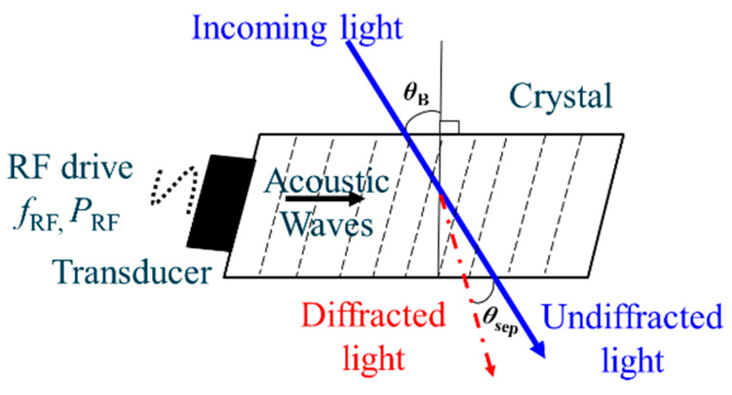
Figure 2.
Block diagram of a AOTF Chain.
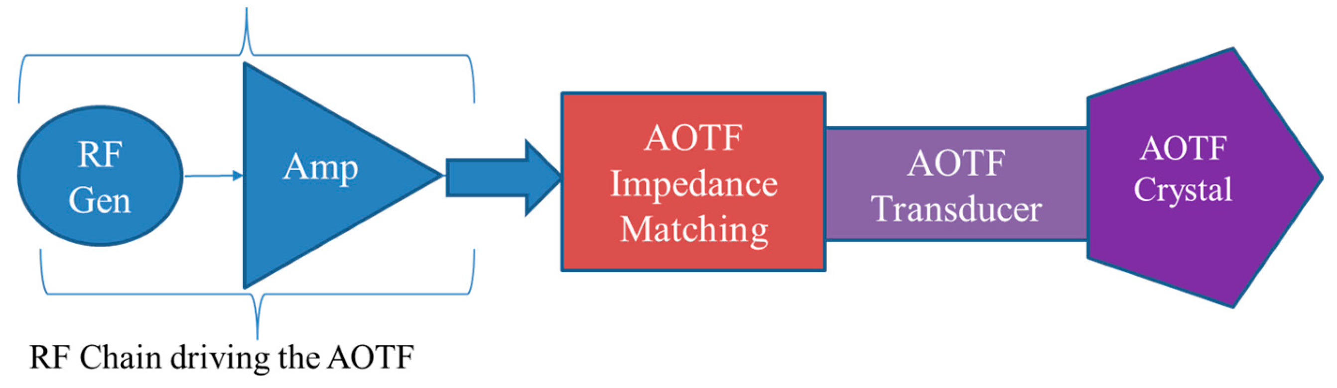
Figure 3.
Normalized voltage and current waveforms (a) Class E (b) Class F.
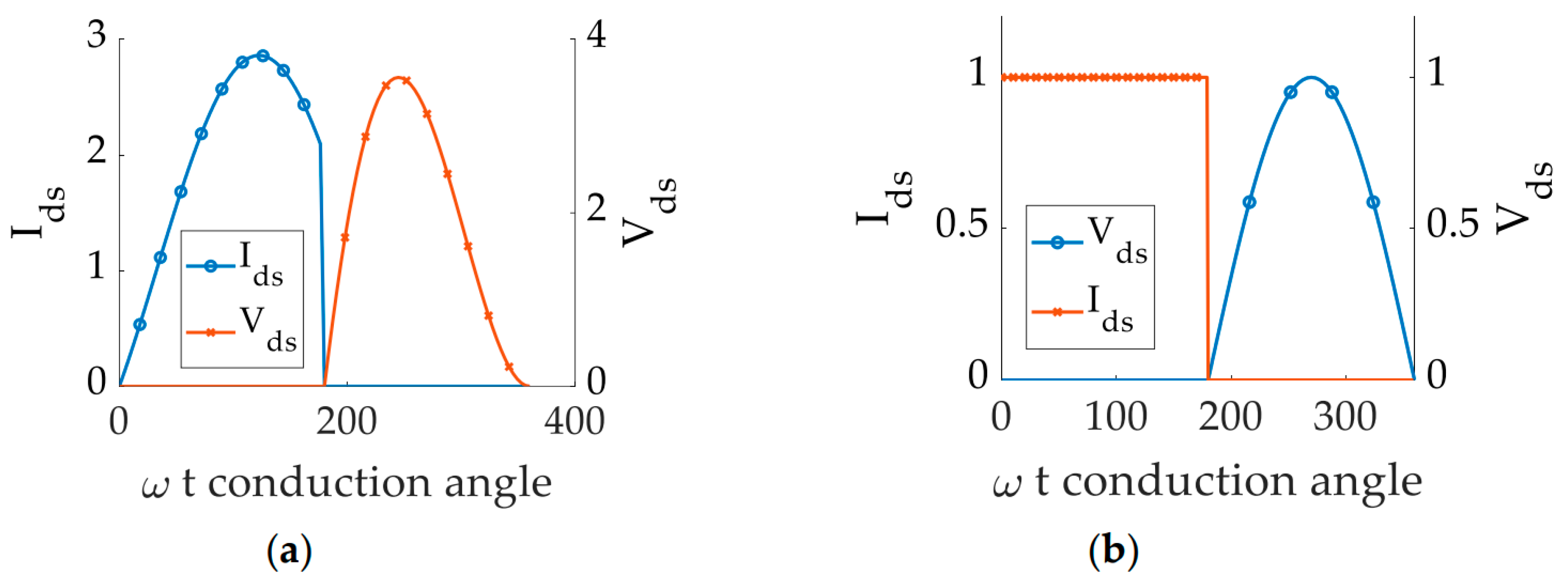
Figure 4.
Class E RFPA with infinite DC feed (a) schematic (b) equivalent circuit.
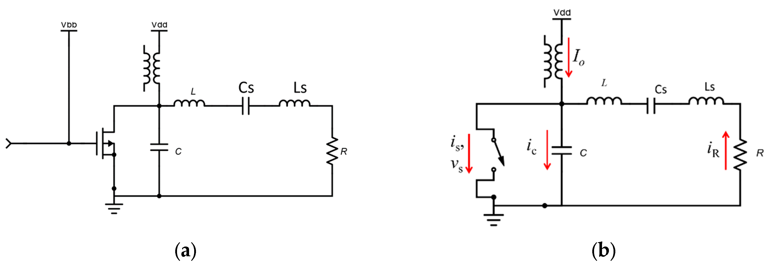
Figure 5.
Class E with finite DC feed (a) schematic (b) equivalent circuit.
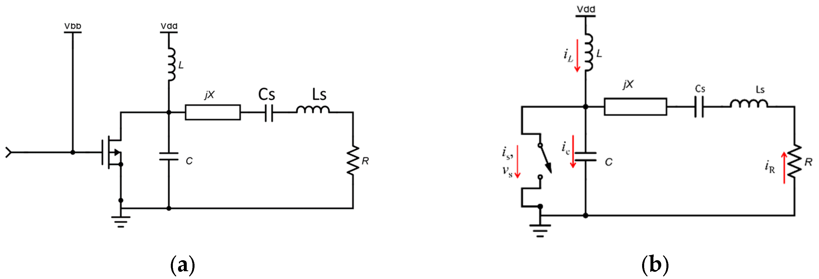
Figure 6.
Efficiency vs PAE (a) with infinite DC feed (Topology 1) (b) with finite DC feed (Topology 2.1, q = 0.5) (c) with finite DC feed (Topology 2.2, q = 1.412).
Figure 6.
Efficiency vs PAE (a) with infinite DC feed (Topology 1) (b) with finite DC feed (Topology 2.1, q = 0.5) (c) with finite DC feed (Topology 2.2, q = 1.412).
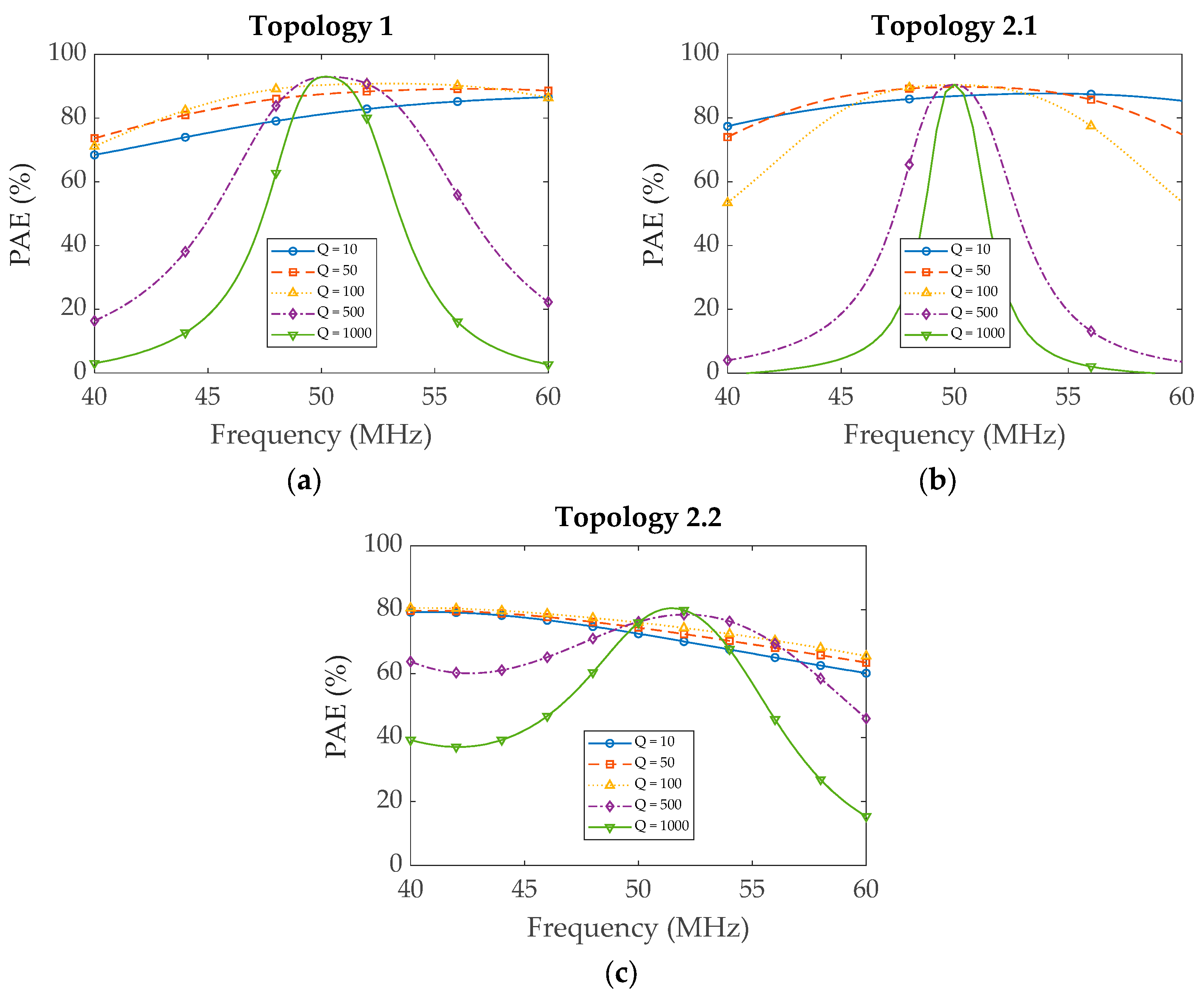
Figure 7.
Load angle vs frequency for all the topologies with varying Q (a) Q =10 (b) Q = 50 (c) Q = 100 (d) Q = 500 (e) Q = 1000.
Figure 7.
Load angle vs frequency for all the topologies with varying Q (a) Q =10 (b) Q = 50 (c) Q = 100 (d) Q = 500 (e) Q = 1000.
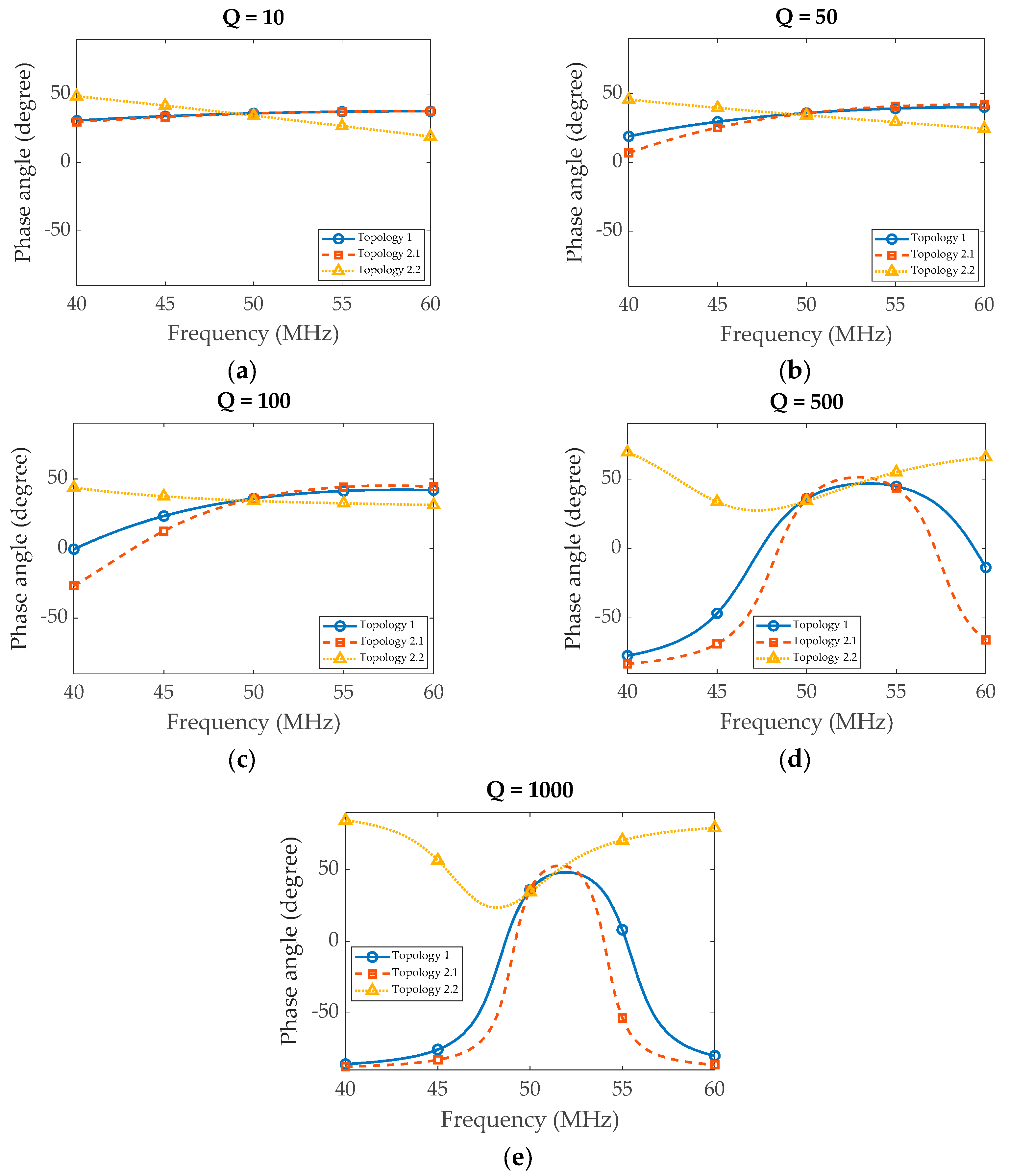
Figure 8.
2nd harmonic tuning.
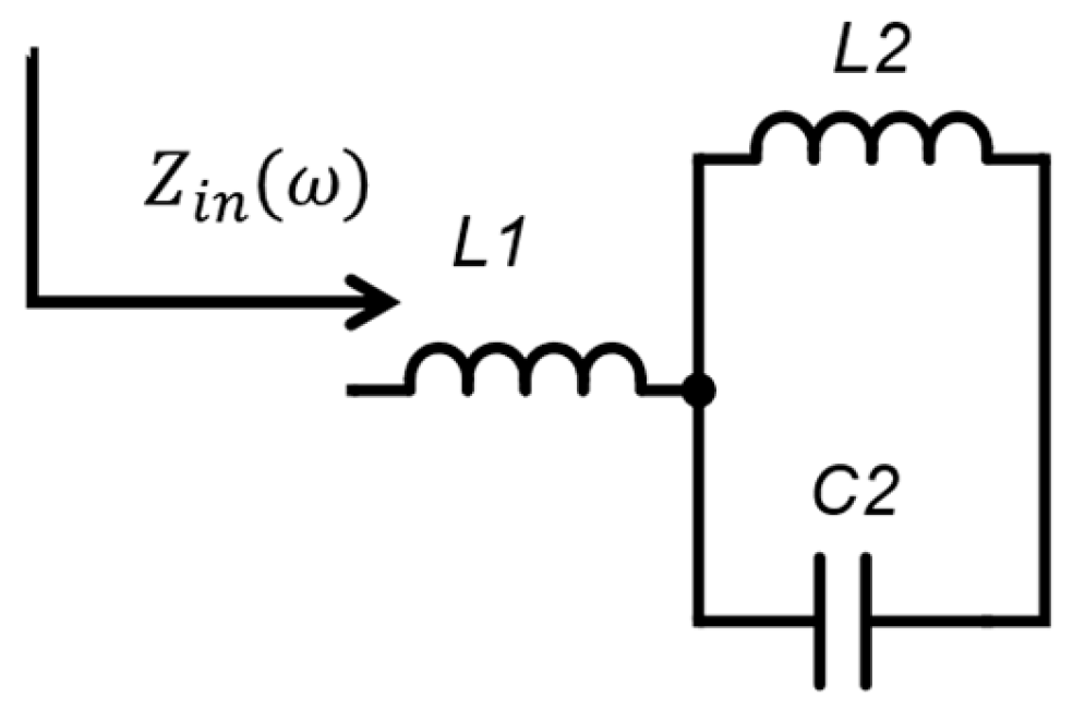
Figure 9.
Frequency dependent load network variation designed for 50 MHz (a) magnitude (b) phase. (H23- 2nd and 3rd harmonic tuning; H2: 2nd harmonic tuning; Topology 2.2: parallel class E).
Figure 9.
Frequency dependent load network variation designed for 50 MHz (a) magnitude (b) phase. (H23- 2nd and 3rd harmonic tuning; H2: 2nd harmonic tuning; Topology 2.2: parallel class E).
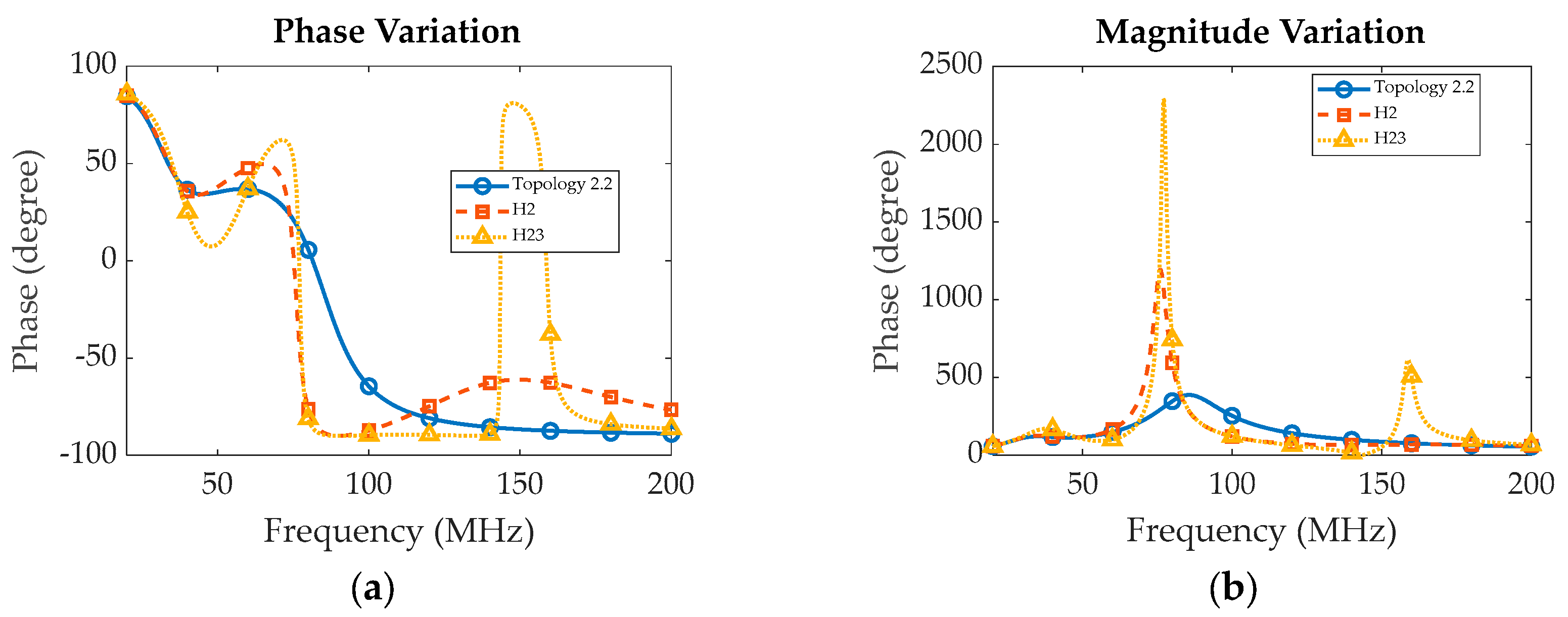
Figure 10.
Ideal simulated voltage and current waveforms for various topologies (H23- 2nd and 3rd harmonic tuning; H2: 2nd harmonic tuning; 2.2: parallel class E).
Figure 10.
Ideal simulated voltage and current waveforms for various topologies (H23- 2nd and 3rd harmonic tuning; H2: 2nd harmonic tuning; 2.2: parallel class E).
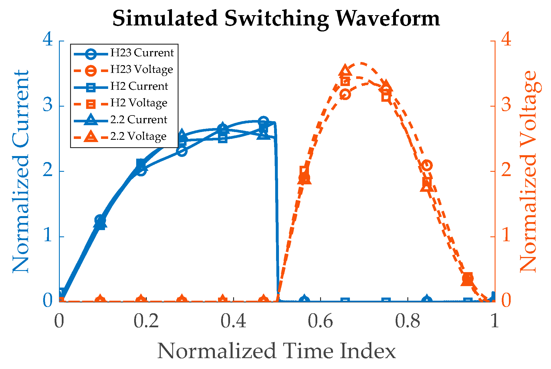
Figure 11.
Schematic of Class E with 2nd and 3rd harmonic tuning.
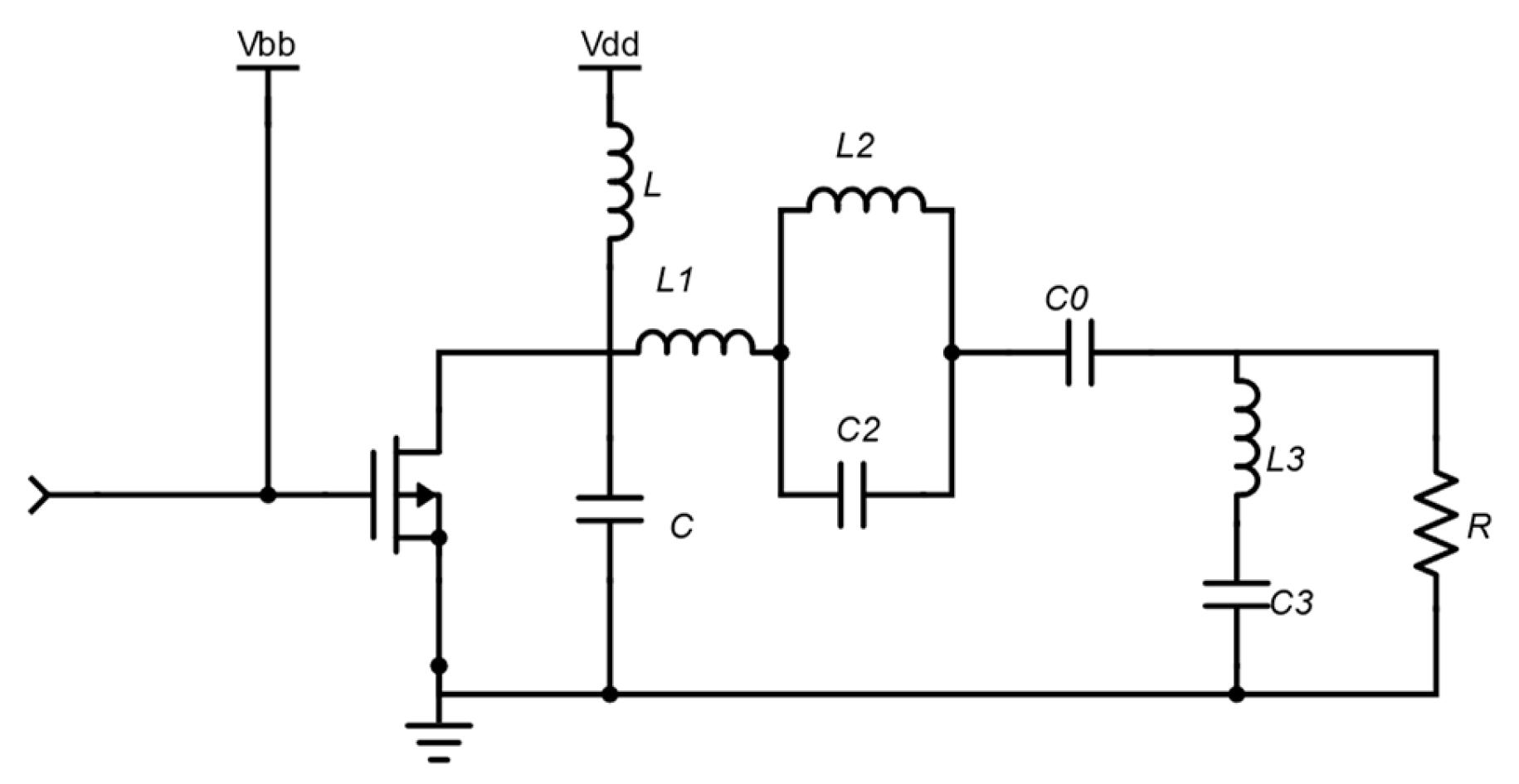
Figure 12.
Simulated power spectrum till 3rd harmonic for the optimized values (a) RFPA designed for 50 MHz (b) RFPA designed for 100 MHz.
Figure 12.
Simulated power spectrum till 3rd harmonic for the optimized values (a) RFPA designed for 50 MHz (b) RFPA designed for 100 MHz.
| Var. | R | C | L | C0 | L1 | L2 | L3 | C2 | C3 |
| Units | Ω | pF | nH | pF | nH | nH | nH | pF | pF |
| 50 MHz | |||||||||
| Ideal | 136.50 | 15.97 | 318 | 22.72 | 167.17 | 208.96 | 53 | 12.12 | 21.22 |
| Opti. | 147.7 | 20 | 362 | 23 | 206 | 395 | 86 | 6 | 14 |
| 100 MHz | |||||||||
| Ideal | 136.50 | 7.98 | 159.02 | 11.36 | 83.58 | 104.48 | 26.52 | 6.06 | 10.61 |
| Opti. | 157.74 | 12 | 109 | 11 | 190 | 113 | 55 | 6 | 6 |
Figure 13.
Simulated PAE vs frequency for the optimized values (a) RFPA designed for 50 MHz (b) RFPA designed for 100 MHz.
Figure 13.
Simulated PAE vs frequency for the optimized values (a) RFPA designed for 50 MHz (b) RFPA designed for 100 MHz.
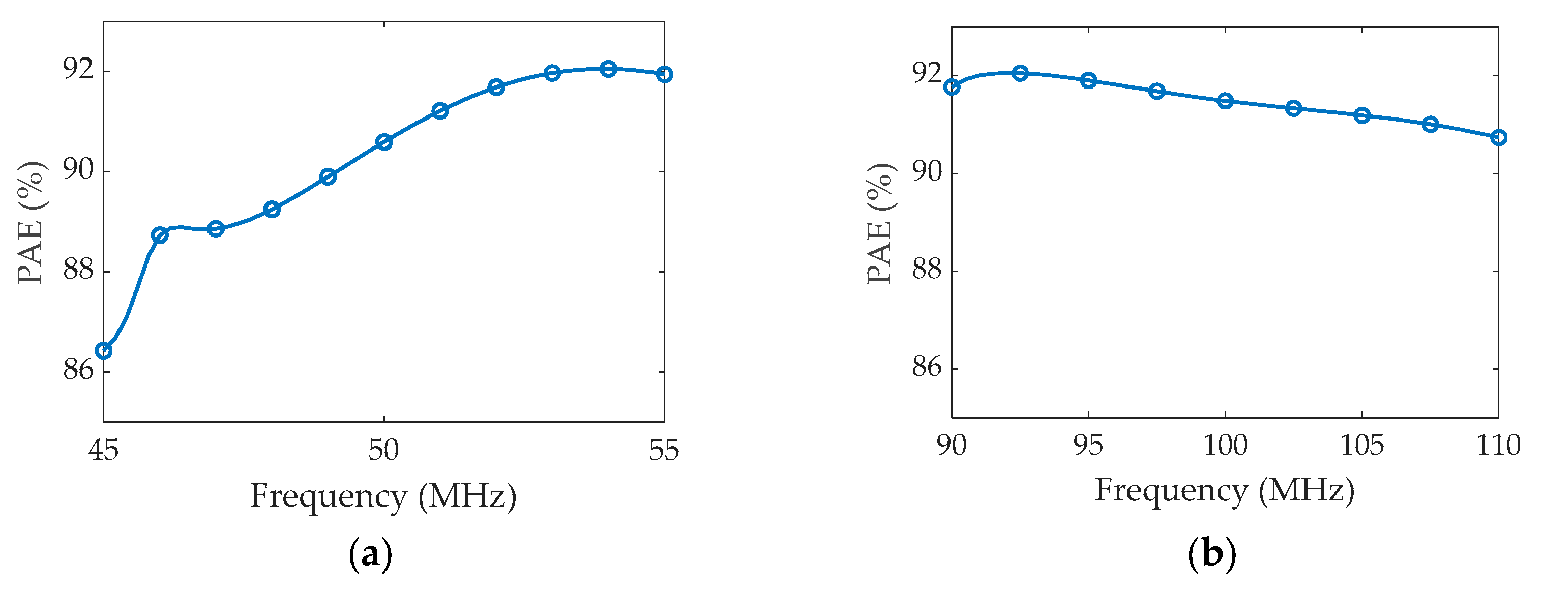

Table 1.
Load network values for different topologies for 1 Watt output power at 50 MHz.
| Values- | R | C | L | Lx |
| Topology 1 | 57.68 Ω | 10.13 pF | - | 211.60 nH |
| Topology 2.1 | 63.50 Ω | 10.62 pF | 3.82 uH | 213.85 nH |
| Topology 2.2 | 136.50 Ω | 15.97 pF | 318.04 nH | - |
Table 2.
PAE and power levels with Q variation.
| Q (50 MHz) | PAE |
Fund. (dBm) |
2nd (dBm) |
3rd (dBm) |
| Topology 1: With DC feed | ||||
| 10 | 81.137 | 29.341 | 18.545 | 9.695 |
| 50 | 87.458 | 29.592 | 16.092 | 4.096 |
| 100 | 90.358 | 29.595 | 13.262 | -0.640 |
| 500 | 92.812 | 29.421 | 2.401 | -14.326 |
| 1000 | 92.896 | 29.370 | -3.220 | -20.309 |
| Topology 2.1: With finite DC feed and q = 0.5 | ||||
| 10 | 78.402 | 31.450 | 20.706 | 12.265 |
| 50 | 87.116 | 31.879 | 16.983 | 4.353 |
| 100 | 89.825 | 31.257 | 13.257 | -1.326 |
| 500 | 91.497 | 31.726 | 1.178 | -15.60 |
| 1000 | 91.561 | 31.690 | -4.620 | -21.655 |
| Topology 2.2: With finite DC feed and q = 1.412 | ||||
| 10 | 76.885 | 28.581 | 18.471 | 13.588 |
| 50 | 76.834 | 28.683 | 18.910 | 12.722 |
| 100 | 80.932 | 29.076 | 18.624 | 8.544 |
| 500 | 90.205 | 29.403 | 7.738 | -9.144 |
| 1000 | 92.711 | 29.349 | 1.504 | -16.058 |
| 1500 | 92.773 | 29.328 | -2.119 | -19.855 |
Table 3.
PAE and power levels with Q variation.
| Var. | R | C | L | C0 | L1 | L2 | L3 | C2 | C3 |
| Units | Ω | pF | nH | pF | nH | nH | nH | pF | pF |
| 50 MHz | |||||||||
| Ideal | 136.50 | 15.97 | 318 | 22.72 | 167.17 | 208.96 | 53 | 12.12 | 21.22 |
| Opti. | 147.7 | 20 | 362 | 23 | 206 | 395 | 86 | 6 | 14 |
| 100 MHz | |||||||||
| Ideal | 136.50 | 7.98 | 159.02 | 11.36 | 83.58 | 104.48 | 26.52 | 6.06 | 10.61 |
| Opti. | 157.74 | 12 | 109 | 11 | 190 | 113 | 55 | 6 | 6 |
Disclaimer/Publisher’s Note: The statements, opinions and data contained in all publications are solely those of the individual author(s) and contributor(s) and not of MDPI and/or the editor(s). MDPI and/or the editor(s) disclaim responsibility for any injury to people or property resulting from any ideas, methods, instructions or products referred to in the content. |
© 2024 by the authors. Licensee MDPI, Basel, Switzerland. This article is an open access article distributed under the terms and conditions of the Creative Commons Attribution (CC BY) license (http://creativecommons.org/licenses/by/4.0/).
Copyright: This open access article is published under a Creative Commons CC BY 4.0 license, which permit the free download, distribution, and reuse, provided that the author and preprint are cited in any reuse.


