
Submitted:
18 July 2024
Posted:
19 July 2024
You are already at the latest version
Abstract
Based on economic feasibility, renewable generators can use pumped hydro storage (PHS) to improve their profitability by performing energy arbitrage under real time pricing (RTP) schemes. In this paper, we present a new method to optimise the size and manage utility-scale wind-PV systems using PHS with energy arbitrage under RTP. The storage in the PHS is used to supply load consumption and/or energy arbitrage. Further, both load supply and power-generating systems are considered, and a genetic algorithm metaheuristic technique is used to perform the optimisation efficiently. Irradiance, wind speed, temperature, hourly electricity price, component characteristics, and financial data are used as data, and the system is simulated in 15 min time steps during the system lifetime for each combination of components and control variables. Uncertainty is considered for the meteorological data and electricity prices. The pump and turbine efficiencies and available head and penstock losses are considered as variables (not fixed values) to obtain accurate simulations. A sample application in Spain is demonstrated by performing a sensitivity analysis of different locations, electricity prices, and costs. The PHS is not worth considering with the present cost of components.
Keywords:
Photovoltaic
; wind turbines
; pumped hydro storage (PHS)
; simulation
; optimisation
1. Introduction
At the utility scale, power generation systems such as photovoltaic (PV) generators or wind farms sell electricity to an AC grid in the long-term market via the daily or intraday market or through a power purchase agreement. At this scale, there are high-load consumers (towns, large factories, residential, commercial, or industrial areas) that can supply their load consumption via the utility grid and/or their own generating systems (e.g. PV and/or wind turbines with or without storage). We study large consumers such as load supply systems (LSS) with their own generating systems that include PV, wind turbines, and PHS storage. Further, we consider power-generating systems (PGS) comprising a PV generator and/or wind turbines with PHS storage, where the objective is maximizing the income generated by selling electricity to the grid. There is no auxiliary load consumption, i.e., the load for auxiliary components is considerably lower than the generated power. At the national utility-scale levels, grid stability and secure load supply suggest the necessity to increase energy storage in the generation mix with a greater presence of renewable energy and a lower weight in the mix of thermal power plants [1]. High PV penetration affects the shape of day-ahead hourly price curves, lowering the daytime electricity prices [2] (‘duck’ shape [3]). In grid-connected systems, PHS is a type of storage that can be used for energy arbitrage: store electricity (pump water from the lower to the higher reservoir) during hours when electricity prices are low (off-peak hours, with low national demand) and use the stored energy (the water from the upper reservoir flows back down through a turbine and generates electricity) to inject electricity to the grid when the electricity price is high (peak hours, with high national demand). Thus, PHS can improve grid stability and load supply security and reduce costs in LSS or increase benefits in PGS. Energy arbitrage with PHS could be profitable (i.e. the increase in benefits attributed to price arbitrage could help compensate for its investment and operational costs) based on the hourly electricity prices, PHS efficiency, and capital expenditures (CAPEX), and operational expenditure (OPEX) costs, [4]. Other PHS benefits for renewable power include curtailment reduction, fast and flexible ramping, frequency regulation, black start, and capacity firming [3]. In addition, PHS can be used for other ancillary services such as steady-state voltage control, fast reactive current injections, and island operation capability [5].
PHS is the dominant technology in electrical energy storage, with 97% of power and 99% of storage energy [6]. The primary advantages of PHS as storage include its technological maturity, long useful life, high overall efficiency, rapid response, and strong power ramping. PHS is the most suitable technology for small islands and mass storage [7], and it has been used for energy storage on islands with high renewable penetration, such as the El Hierro [8] and Feroe islands [9]. PHS is the most suitable technology for the seasonal storage of electrical energy. Hunt et al. (2020) [10] showed that more than 79% of global electricity consumption in 2017 could be stored in PHS at a cost of less than US$50/MWh. Existing PHS plants in electrical systems consume electricity during off-peak hours (pumping water) and inject electricity using the stored energy into the grid during peak hours, thereby contributing to grid services. Further, they operate in an open (one or more reservoirs are connected to a natural body of water) or closed loop (reservoirs are separate from natural waterways) [7]. Traditionally, PHS operated at a fixed speed [11] although variable-speed systems were gradually incorporated [12,13].
Mountainous countries show high potential for pumped storage hydropower (for example, Nepal [14]). In many mountainous countries, and specifically in Spain, there is considerable potential for reusing traditional hydroelectric power plants through the aggregation of pumping systems, and there is also the possibility of expanding existing pumping plants by incorporating new groups with the same hydraulic infrastructure [15]. Further, using low-head applications can make PHS usable in regions where it is not feasible traditionally [5]. Underground pumped storage hydropower (UPSH, also called sub-surface pumped hydro storage, SSPHS) can avoid the environmental problems of installing new massive PHS plants using underground deposits in caverns or in abandoned mines (use of water from mine drainage for generating electrical energy through a reversible purification plant, thereby allowing the regeneration of mining environments). Although this technology is still in the development phase [16], there are already projects for mining basins in Germany, the United Kingdom, Spain, China [17] and USA [18]. Other nonconventional technologies are also being evaluated, e.g. the use of canals or streams at different heights or deposits on the seabed [19]. In addition, there are innovative projects that involve seawater pumping, in which the lower reservoir is the sea [20,21], with existing projects in Japan, Ireland and Hawaii [18]. Renewable generation can be installed near existing PHS plants, operating in a similar way as a traditional power plant (energy management and arbitrage) and exploiting the existing grid connection infrastructure. Floating photovoltaic generation can also be added to the existing PHS reservoirs [22].
Rehman et al. [7] presented a technological review of renewable power storage using PHS. Barbour et al. [23] reviewed the developments in relevant international electricity markets, and Lian et al. [24] reviewed studies on hybrid renewable systems, including those that used PHS. Ali et al. recently investigated the drivers of and barriers to PHS [25]. Javed et al. presented an extensive review of solar and wind power generation systems with PHS [19].
The literature review indicates that most previous optimisation articles on PV-wind-PHS systems are related to off-grid systems. In addition, the literature review indicated that in PV-wind-PHS optimisation studies, the head dependence of water-power conversions and the variability of the friction losses and pump-turbine efficiency are neglected in the studies on PV-wind-PHS optimisation, assuming fixed constant values.
Toufani et al. performed a full review to address the uncertainty in the optimisation of PHS [26], concluding that only a few studies considered uncertainties in PHS sizing, while even fewer studies focused on long-term planning.
The majority of studies on grid-connected PV-wind-PHS optimisation attempted to optimise the daily operation (short-term). Thus far, few studies optimised the size of the PV-wind-PHS system; however, they did not consider energy arbitrage, and only considered the grid to inject surplus energy (which cannot be used by the load that is not stored) or to import the energy required by the load that cannot be covered by the system.
Eliseu and Castro [27] optimised the day-ahead operation of a Wind-PHS system with two different objectives: maximisation of the market profit or generation of constant firm output power. Abadie and Goicoechea [1] presented a stochastic model for evaluating the effect of an optimally managed PHS power plant using certain price ranges for pumping and others for generation. They optimised energy management, but not component size, thereby considering the PHS global efficiency for a fixed value of 80%. Nassar et al. [28] optimised the size of a PV-wind-PHS system for supplying the load of an urban community in Libia, injecting surplus energy into the grid (which cannot be used by the load or stored) and consuming the energy that cannot be supplied by the system from the grid. Variable penstock losses were considered (assuming laminar flow); however, the pump and turbine efficiencies were considered constant. In addition, fixed electricity prices were used to sell or purchase electricity from the grid. Gao et al. [17] optimised the daily operation of a PV-wind-PHS (PHS mine in China), thereby reducing the volatility of the power injection to the grid and increasing the benefits; however, they did not consider variable losses in the pump, turbine, or penstock. Recently, Al-Masri et al. [29] presented the optimisation (minimisation of grid-usage factor) of the different combinations of PV, wind, and PHS grid-connected systems with load consumption, which includes the variability of the friction losses and variable height, water reservoir evaporation, and seepage in the simulations; however, the pump and turbine efficiencies are considered as fixed values, and the energy management strategy is simple (injected into the grid only when there is surplus energy that cannot be stored in the reservoir), and the electricity grid price is a fixed value. Yin et al. [30] presented a method for the multi-objective minimisation of power mismatch and the maximisation of revenues in offshore wind-PHSs, using accurate models for wind generation (including the wake effect) and considering hourly periods for the electricity price. However, simple models for the PHS were used (fixed efficiency for the pump-turbine performance including friction losses and no variable head).
Recently, Naval et al. [31] showed the optimisation of the operation of a grid-connected PV-wind-PHS system that must supply a specific load consumption for one year. The optimisation of the monthly strategy maximise the benefits using PHS to meet the demand not covered by renewable sources and injecting surplus energy into the grid (not considering arbitrage). They used hourly prices of the Spanish wholesale electricity market in 2019, while considering fixed values for pump turbine performance, including friction losses and no variable head.
To the best of our knowledge, none of the previous studies considered the use of PHS for arbitrage in grid-connected systems with load consumption under a real-time pricing (RTP) scheme for the electricity price. In this study, we consider the use of PHS for arbitrage under electricity RTP, optimising the component size (PV, wind, pump turbine, and reservoir) and set points for arbitrage and management. Further, we used advanced models that have not been used in previous studies related to the optimisation of renewable – PHS systems. The main features of this work are provided below:
Both LSS, where the objective is minimising the electricity cost of the load supplied, and PGS, where there is no load and the objective is maximising income from selling electricity to the grid, are optimised.
Two different energy arbitrage systems are used: allowing or not buying energy from the grid during low RTP price periods to store energy in the pumped water. Further, the case without PHS is optimised for comparing the optimal results with and without PHS.
Each combination is simulated in time steps of 15 min during the lifetime of the system (typically 25 years).
Unlike most previous studies, we consider uncertainties in electricity prices, solar irradiation, and wind speed over the entire lifetime of a system. Further, an increase in load consumption during the system lifetime was considered.
The RTP electricity price is updated every year considering the effect of the increase in renewable power in the national electrical mix (‘duck curve’ of the electricity price profile).
The performance decay of equipment during the years of the system lifetime is considered.
Unlike most previous studies, we used accurate nonlinear models for all components and considered variable pump and turbine efficiencies (variable speed); variable head (attributed to changes in the water level in the upper and lower reservoirs); variable losses in penstocks, water reservoir evaporation, and seepage; and variable efficiency of the PV inverter.
We optimised not only the size of all components, but also four variables related to the load supply and energy management for arbitrage (which helps decide the priority to supply the load using the grid or storage, when to store energy, and when to inject energy into the grid).
A genetic algorithm (GA) based metaheuristic technique was used for efficient optimisation.
To the best of our knowledge, none of the previous studies included all these features simultaneously.
The remainder of this manuscript is organised as follows: Section 2 presents the modelling approach for the simulation and optimisation of the system. Section 3 presents the computational results and discussion, including the validation of the simulation approach compared to the results of a previous publication and the optimisation of representative cases with sensitivity analysis. Finally, the conclusions are presented in Section 4.
2. Modelling Approach
Figure 1 shows the PV-wind-PHS. In this study, we expanded the megawatt hybrid maximizing by genetic algorithms (MHOGA) [32,33] software to perform simulations and optimisations.
We consider two systems:
LSS (Figure 1): In this system, electrical load must be supplied during every time step t of the entire system lifetime. The system can be applied to a small town or residential, commercial, or industrial area. Electricity is supplied by means of the grid and renewable-PHS system, and the objective is maximizing the electricity cost (maximizing net present cost, NPC) of the load supplied.
PGS: In such systems, there is no load demand (or the load demand is very low only for the auxiliary consumption of the power system). The objective of the owner of the renewable-PHS power-generating system is maximizing the benefits obtained by selling electricity to the grid (maximizing the net present value, NPV). It would be a specific case of LSS considering no load ( ) or low load (for the auxiliary consumption of the PGS).
Two different types of systems were considered for energy arbitrage (Table 1): Type A (allowed to purchase energy from the grid for energy arbitrage) and Type B (not allowed to purchase energy from the grid for energy arbitrage; purchase is allowed only for the load supply when it is required).
Once the system type was defined, different combinations of components (PV generator, wind turbines, pump turbine, and reservoirs) and control strategies were simulated during the system lifetime in time steps of 15 min and evaluated.
For each time step, the energy balance was determined based on the type of system and different variables. Input variables for each time step t are (Figure 1) maximum grid power , load consumption , PV output power , wind turbines output power (W), water volume of the upper and lower reservoirs, and (m3), electricity price (purchase to the AC grid price and sell to the AC grid price), and and (€/kWh).
The set points are listed below:
High limit of electricity price for energy arbitrage (). If the electricity price (purchase or sale price, depending on project type A or B, respectively) is higher than this limit, the priority is injecting electricity into the grid, including hydropower generation, at its maximum allowed power.
Low limit of electricity price for energy arbitrage (). If the electricity price is lower than this limit, a pump is used to store water in the upper reservoir. Depending on the type of project (A or B), the pump runs at its rated power (consuming electricity from the grid, if needed) or with the power supplied by the net renewable power.
Limit of the purchase price for the electricity to supply the net load using the grid (if the electricity price is lower than this setpoint) or hydro turbine (if the price is higher): . This setpoint has no meaning in the PGS if there is no load. In addition, during the time steps when arbitrage (charge or discharge) was selected, this setpoint had no meaning.
Minimum hydro turbine load: Minimum percentage of the hydro turbine rated power to supply the net load ().
For each time step, the net load is defined as the load minus the renewable power.
The net renewable power is expressed as
The energy arbitrage performances of the two types of systems are explained as follows (see Table 1).
Type A: Energy arbitrage is considered during each time step. If the purchase electricity price is higher than the high set point () → ‘arbitrage: discharge’, the priority is injecting the (sell) electricity to the grid (net renewable generation + hydro turbine at maximum power). If the purchase electricity price is lower than the low set point () → ‘arbitrage: charge’, the priority is storing the energy (to pump water with renewable surplus power). If the renewable surplus power is lower than the pump nominal rated power (), the difference is purchased from the grid to run the pump at rated power. If the purchase electricity price is between the two setpoints → ‘no arbitrage’ (dead band for arbitrage): if there is surplus power, it is sold to the grid; if there is net load, it is covered by the hydro turbine only if the purchase electricity price is higher than the load set point limit () and the net load is higher than a specific percentage of the turbine nominal rated power ( > ). In this way the hydro turbine is used to supply the net load (using stored energy) only when the purchase price and power are high (avoiding turbine low efficiency at low power).
Type B system (not allowed to purchase electricity from the grid for arbitrage). Unlike Type A, it is not allowed to purchase electricity from the grid for arbitrage in this system (purchasing electricity from the grid is allowed only to supply the net load). In this type of system, the selling price is the electricity price used for comparison with arbitrage setpoints. For each time step, the energy arbitrage operates as follows: If the sell electricity price is higher than the high set point () → ‘arbitrage: discharge’, the priority is injecting (sell) electricity to the grid (net renewable generation + hydro turbine maximum power). If the sell electricity price is lower than the low set point () → ‘arbitrage: charge’, the priority is storing energy (to pump water just with the renewable surplus power, not buying electricity to the grid). If the sell electricity price is between the two setpoints → ‘no arbitrage’ (dead band for arbitrage): same as in type A.
For both cases, the maximum grid power () limits the power purchased and sold to the AC grid.
1.1. Simulation
Each combination of components and control strategy is simulated during the lifetime of the system in steps of 15 min.
1.1.1. PV Model
Global hourly irradiation data over the tilted surface (W/m2) can be imported from the measured data or downloaded from the PVGIS [34], Renewables Ninja [35], and NASA [36] databases. The uncertainty is considered in the irradiance for each hour (h) of each year (y) of the system lifetime , which is obtained by multiplying by a random number that follows a normal distribution with mean 0 and standard deviation . Given the hourly irradiance, the irradiance in 15-min time steps G(t) (W/m2) is calculated using a first-order autoregressive function.
The AC PV generator output at time t (year y), (W), represents the minimum of the output of the PV (considering the inverter efficiency, ) and the PV inverter-rated power (nominal AC output power, ).
where , , , α, ), and , and (°C) represent the rated DC peak power of the PV generator, PV annual reduction factor due to degradation, efficiency factor (dirt, wire losses…), power temperature coefficient (%/°Cirradiance and cell temperature under standard test conditions (1000 W/m2 and 25 °C), respectively, and
cell temperature during time t, respectively, which is expressed as
where (°C) represents the ambient temperature and NOCT (°C) represents the nominal operation cell temperature.
1.1.1. Wind Turbine Model
Hourly wind speed data for an entire year can be imported or downloaded from online databases. The wind speed for each 15-min time step was obtained using a random number (to consider the uncertainty) and first-order autoregressive function model. If the hub height zhub (m) is different from the anemometer height zanem (m), the wind speed at the hub height whub(t) (m/s) is obtained by converting the measured wind speed w(t) (m/s) at the anemometer height considering the surface roughness length z0 (m) based on
The wind turbine output power curve supplied by its manufacturer is measured in standard conditions (temperature 288.15 K, sea level, and air density ρair_0 = 1.225 kg/m3). For each time step, the wind turbine output curve was converted to the air density of the time step ρair(t) (kg/m3) by multiplying with the relationship ρair(t)/ρair_0. Turbines with pitch control maintained their nominal power () without any changes, as shown in Figure 2.
The wind turbine output power (W) at time t for each wind speed is obtained as
where represents the output power curve (power vs. wind speed ) of the wind turbine when it is new (year 0) under standard conditions; represents the wind turbine annual reduction factor owing to degradation ([37]); represents the efficiency owing to losses in wires, switches, etc.; and represents the rated wind speed of the wind turbine (in Figure 2, 15 m/s).
Several wind turbines can work in parallel; in this case, the total output power is calculated considering the wake effect model proposed by González-Longatt [38].
1.1.1. Pump Model
Variable-speed reversible pump turbines are considered in this study. For each time step, the control strategy determines the value of the pump input power (W), which cannot be higher than the nominal rated power () depending on the type of system and on the different variables (Section 2, Table 1). The pump flow rate (water taken from the lower reservoir and stored in the upper reservoir) depends on the pump efficiency and head. The pump model [39] calculates the flow rate of the pump (m3/s) as a function of the input power (first term in Equation 8). The second term of Equation 8 shows that the pump flow rate cannot exceed the nominal flow rate (m3/s). The third and fourth term of that equation show that, at the end of the time step (after = 15 · 60 = 900 s, which corresponds to the time step of 15 min) the lower reservoir volume (m3) cannot be lower than its minimum allowed (m3), and the upper reservoir volume (m3) cannot be higher than its maximum allowed (m3).
where represents the pump efficiency (which includes the motor efficiency) and is a function of , which can be found in the pump technical datasheet; ρ represents the water density (ρ = 997 Kg/m3 at 25 °C), g represents the gravity acceleration (g = 9.81 m/s2), and (m) represents the pump head, which is the sum of the static head and head loss of the pump mode .
The static head is the difference in the water level of the upper and lower reservoirs, which considers the difference in heights between the minimum level of the upper reservoir and maximum level of the lower reservoir (), and the variations over the minimum level of the upper reservoir and below the maximum level of the lower reservoir (Figure 1).
The water level in the upper reservoir can be calculated by assuming that the reservoir has a cuboid shape.
where represents the maximum height of the water in the upper reservoir (m). The variation below the maximum level of the lower reservoir can be calculated by assuming that the lower reservoir has a cuboid shape given by
where represents the maximum volume of the stored water in the lower reservoir (m3) and represents the maximum height of the water in the upper reservoir (m).
𝐻𝑃(𝑡)=𝐻𝑃𝑆(𝑡)+𝐻𝑃𝑙(𝑡).
𝐻𝑃𝑆(𝑡)=𝐻𝑑𝑖𝑓𝑓+𝐻𝑈𝑅𝑡+𝐻𝐿𝑅𝑡.
The head loss of the pump mode represents the hydraulic losses of the pump mode because of the friction between the water and inner surface of the pipes and fittings. is calculated as a function of using the Darcy–Weisbach equation [39]
For laminar flow, the friction factor (f) is calculated as x
where represents the Reynolds number.
For turbulent flow (normal in PHS systems), an approximation of the Colebrook equation (Haaland equation) is used.
where , , and , ε, and represent the total resistance coefficient, coefficient resistance of the pipe, coefficient resistance of the fittings, water speed (m/s), pipe diameter and pipe length between the pump and the reservoir (m), absolute roughness (m), and dynamic viscosity of water (Pa·s), which depends on temperature, respectively.
1.1.1. Turbine Model
The turbine is the same as the pump (pump-turbine reversible machine); therefore, the turbine pipe diameter () and length () are the same as those defined for the pump ().
For each time step, the control strategy determines the hydro turbine output power (W), which is limited to the maximum value .
The maximum hydro turbine output is limited by its nominal rated power (W) and nominal flow rate (m3/s). Further, at the end of the time step, the lower reservoir cannot exceed its maximum volume (m3) and the upper reservoir volume cannot be lower than its minimum value (m3).
The turbine flow rate (obtained from the upper reservoir and stored in the lower reservoir) depends on the turbine efficiency and turbine head. The turbine model [39] calculates the flow rate of the turbine (m3/s) as a function of the input power, which cannot be higher than the nominal flow (m3/s). At the end of the time step, the lower reservoir cannot exceed and the upper reservoir volume cannot be lower than.
where is represents turbine efficiency (which includes the multiplier efficiency and the generator efficiency) and is a function of the flow, which can be found in the turbine technical manual. Further, (m) represents the turbine head, which is calculated as the static head in turbine mode minus the head loss in the turbine mode .
A pump-turbine reversible machine is considered, the static head is defined in the same manner as that for the pump (Equation (10)). The loss in the turbine mode is calculated using the same equations as those for the loss in the pump mode (Equations (13)–(19)) using the turbine flow rate ().
1.1.1. Water Volume in the Reservoirs
The water volumes (m3) in the upper and lower reservoirs at the next time step are calculated as
where and (m3) represent the incoming water minus the outgoing water from the reservoir (apart from the pump and turbine flow) for the upper and lower reservoirs, respectively, which can be calculated based on the geographical features of the area, including losses caused by evaporation and seepage.
The maximum stored energy depends on the maximum volume of the upper reservoir and static head, and it is given by
where represents the average static head in the turbine mode.
The duration of the upper reservoir () represents the time (h) at which the upper reservoir can supply the nominal flow of the turbine (PHS time of full-capacity operation in generation mode).
1.1. Optimisation
The software simulates different combinations of possible components in time steps of 15 min during the system lifetime LifeS (usually 20–25 years, defined by the user): the PV generator (including its own inverter), wind turbine group (size and number of wind turbines), pump-turbine reversible unit, and water reservoir size. Further, it considers four set points for control, as detailed in Section 2 and Table 1.
Considering a system lifetime of 25 years, the number of time steps simulated for each combination is 876,000 (25 × 365 × 24 × 4). Considering the nonlinear characteristics of many components (PV inverter efficiency, wind turbine output curve, pump-turbine efficiency, penstock losses, etc.), optimisation cannot be performed by the classical methods or MILP. In this study, GA metaheuristic techniques were used for the optimisation. The two GA were considered in the optimisation: a main algorithm to determine the optimal configuration of the components, and a secondary GA to determine the optimal control.
Five variables are optimised with the main GA.
where , , , , and represent the code for the PV generator type (including its own inverter), code for the wind turbine type, number of wind turbines in parallel, code for the pump-turbine reversible machine type, and water storage duration defined in Equation 28, respectively. In each case, the penstock diameter was calculated to obtain the specific water speed for the nominal flow of the pump/turbine.
For each combination, the maximum reservoir volume is calculated as follows: is obtained from the (Equation (28)), and the is proportional to the upper reservoir by a factor () that depends on the design conditions.
The secondary GA optimises the control strategy, which is composed of four setpoint variables (explained in Section 2).
For each combination of the main GA, the secondary GA is run to obtain its optimal control, simulation, and evaluation of a number of combinations of the four set-point variables.
In the LSS, the objective of the optimisation is to find a combination of components and a control strategy to minimise the NPC
Under the constraint that the unmet load (%) must be lower than the maximum unmet load allowed (),
In the PSS systems, the objective of optimisation is to find a combination of components and a control strategy to maximise the NPV.
where NPV is the opposite of the NPC.
1.1. Economic Results Calculation
The NPC of each combination of components and the evaluated control strategy is computed considering all costs during the system lifetime: the CAPEX and OPEX of all components of the system, their replacement cost during the system lifetime, and cost of electricity purchased from the AC grid. All cash flows are converted to the present moment using a discount rate. In addition, the income from selling the electricity to the grid during the lifetime of the system was considered (negative values as income) [33].
where I and Inf represent the annual nominal interest or discount rate and annual inflation rate, respectively; OPEXj represents the annual OPEX of component j at the beginning of the system lifetime (year 0). For the pump turbine, we consider the start-up cost (a cost is considered each time the pump turbine starts to work), which will be added to the annual OPEX. NPCrep_j represents the sum of the present costs because of the replacement of component j (PV, wind turbine group, pump/turbine, and reservoir) during the system lifetime minus the incomes attributed to the residual life of all components at the end of the system lifetime. Incsell_E_y represents the income from the electricity sold to the AC grid during year y. Costpurch_E_y represents the cost of electricity purchased from the AC grid during year y (1…LifeS). TAXy represents the cost of payable taxes related to project benefits: revenues minus operational expenses, interest, depreciation, and amortisation multiplied by the applicable tax rate TR (%), calculated as shown in ref. [40].
In the LSS, the levelised cost of energy (LCOE) is the cost per kWh consumed and sold to the grid.
where and represent the 15-min load and energy sold to the grid during year y, respectively.
In the PGS, the net present value (NPV) of each combination of components and the control strategy evaluated is the opposite of the NPC.
In PGS systems, the LCOE is the generation cost of kWh injected into the grid, which is calculated as
where represents the sum of the total present costs of the system over its lifetime (NPV minus income).
1.1. Electricity Price
The PV-wind-PHS system is assumed to be an electricity price taker, and a real-time pricing (RTP) model is considered. The effect of the change in the hourly profile of the day caused by the increase in PV penetration (‘duck curve’) and the increase in wind penetration are considered for estimating the future electricity prices. The selling electricity price in year y is calculated as [41]
where represents the sell electricity price of hour h (0… 8760) of year y. represents the PV factor to consider the price reduction in the future hourly price profile attributed to an increase in PV penetration ‘duck curve’ depending on the average irradiance of hour h of year 1 (W/m2). represents the wind factor to consider the price reduction in the future hourly price profile caused by an increase in wind generation and represents the annual inflation rate for the electricity price. The uncertainty in electricity price was considered using a random number with a mean and standard deviation for calculating the annual electricity price inflation rate for each year y.
The price calculated in the previous equation refers to year 0 (beginning of the system lifetime); therefore, the price considered for year will be updated (increased due to inflation) by a factor . The purchase price of electricity is affected similarly. The electricity (purchase or sell) price set points are updated each year with electricity price inflation so that the electricity price of each hour of each year is compared to their updated values.
3. Computational Results and Discussion
We compare the results obtained using our model with those of a previous study to validate the model (Section 3.1). We optimise the LSS and PGS; in both cases, we consider two types of projects in terms of arbitrage (types A and B) and compare them to the optimal system without PHS. A sensitivity analysis of the most important variables is presented and the effects of the set-point control variables are analysed.
3.1. Model Validation
The optimal LSS system found by Nassar et al. [28] (the lowest LCOE system) was simulated, and the results were compared. This system for electrifying an urban community (1.2 MW peak power and 6.14 GWh annual energy consumption) in Southern Libya, and it consists of 1,000 kWp solar PV array and 5,000 kW wind turbines farm coupled with a PHS of 166,532 m3 volume capacity (upper reservoir), fixed static head of 70 m, and reversible pump-turbine of 1 MW with a fixed value of 88% total efficiency. Purchasing electricity from the grid is not allowed; however, surplus energy (when the upper reservoir is full and no more energy can be stored by PHS) can be sold (at a fixed price). Nassar et al. also considered the AC grid to be sufficiently large to absorb all excess energy (no grid limit); the water through the penstock was laminar flow (which is not usual); and the water reservoir evaporation and seepage were neglected. The load distribution during the year was estimated using the data shown in Ref. [28]. As Nassar et al. did not show the values of , , , and ε, we estimated and , , and , thereby calculating the penstock losses without any previous assumption of turbulence. In addition, we assume that the lower reservoir has the same capacity as the upper reservoir.
Table 2, first and second rows, shows the main results obtained by Nassar et al. [28] and our results, respectively. The results obtained by Nassar et al. [28] and our results are almost the same. Unmet load obtained by Nassar et al. was reported to be 0% (all demand covered), while in our case, we found 0.4% (unmet load is possible because it is not allowed to purchase energy to the grid). This small difference in the unmet load can be attributed to the distribution of the load during the year, which in our case was estimated from the average monthly values shown in ref. [28]. However, it is impossible to exactly reproduce the load profile of all years because of penstock losses (because of the assumptions of length, diameter and pipe data), considering that Nassar et al. assumed laminar flow (which is not true for reasonable diameters).
Although Nassar et al. did not consider this, the PV and wind turbine power decay over the years in a real system. In addition, it is common for the load demand to increase over time. Further, the variable efficiencies of the turbine and pump modes (variable-speed Francis pump turbine, efficiency in Figure 3 obtained from Refs. [42] and [43]) and variations in reservoir height must be considered to obtain accurate results.
We simulated the same system considering variable head (assuming
, same maximum height for both reservoirs) for 25 years considering a PV power decay of 0.5% annually [44], wind turbine power decay of 0.2% annually [37], and increase in load consumption of 0.5% annually (Figure 4). No uncertainty was considered in the irradiation, wind speed, or electricity price inflation rate (there was no change in annual values during the years).
The results are shown in the last row of Table 2 (the average, minimum, and maximum values for different years are shown for each variable). The annual energies of the different components during the system lifetime are shown in Figure 5. The load increases with years, whereas the PV and wind energies decrease, consequently causing the pump and hydro turbine energies to increase with the years. As the years go by, there are more hours of the years when the load cannot be supplied by PV and wind, and therefore, more energy is required from the hydro turbine and by the pump to recover the upper reservoir volume. Another consequence is that the amount of energy sold to the grid (dashed line) decreases with time. In addition, the unmet load increases with years, reaching 2.35% in the 25th year, which could be inadmissible. This example shows the importance of simulating the system lifetime and considering the real power decay of renewable sources, increase in load, and variable losses and efficiencies.
3.1. Optimisation of an LSS System (System with Load Consumption)
The LSS system for the electrification of the urban community in Libya shown by Nassar et al. [28] (Section 3.1) was optimised to minimise the NPC. We optimise the system without PHS (only the hybrid PV-wind system) and the system with PHS considering the two types of arbitrage operations (A and B) shown in Table 1. There is no RTP electricity pricing in Libya, and therefore, we changed the location to Zaragoza (Spain) using the Spanish 2023 RTP.
The same assumptions specified in Section 3.1 are assumed in this section (increase in an electrical load of 0.5% annually, decay in the PV generation of 0.5% annually, decay in the wind generation 0.2% annually, and pipes, fittings, and reservoir assumptions). In this case, we considered the uncertainty in the irradiation, wind speed, and electricity price inflation rate. Further, we considered a limit for the electricity purchased or sold to the grid (grid limit) of 2 MW (fixed value for all years). The purchase of electricity by the grid is allowed, and the constraint of the maximum unmet load allowed is set to 0.
3.1.1. Resources
Zaragoza (Spain) (41.66 °N, 0.88 °W) was selected as the location of the system. The PV module slope was 35°, which is optimal for maximising the annual irradiation over the tilted surface (2,049 kWh/m2). Hourly irradiation (Figure 6) and temperature data were downloaded from PVGIS in 2020.
The uncertainty of the hourly irradiation for each year was obtained using a standard deviation = 5% (this value was obtained by analysing the data from 1981–2021 downloaded from NASA [45]). Figure 7 shows the variation in the annual irradiation over the average.
Wind speed is determined at a height of 53 m (hub height of the wind turbines is defined later) and downloaded from Renewables Ninja (Figure 8), which helps obtain an average of 6.96 m/s with a 2.9 form factor of the Weibull distribution that best fits the data. The uncertainty of the hourly wind speed for each year was obtained using a standard deviation = 2.7% (obtained after analysing the variation over 10 years). Figure 9 shows the variation in the annual average wind speed over the average, in percentage.
3.2.2. Electricity Price
At the beginning of the system (first year), the RTP of Spain in 2023 was considered for the selling electricity prices. Figure 10 shows the hourly selling electricity price in the first year, with an average of 0.087 €/kWh, a maximum of 0.22 €/kWh, a minimum 0 €/kWh, and a standard deviation of 0.041 €/kWh.
The daily difference between the maximum and minimum selling electricity prices should be known as the profitability of arbitrage depends on these differences. The values for the first year are shown in Figure 11, with an average of 0.0733 €/kWh, maximum of 0.19 €/kWh, minimum of 0.00433 €/kWh, and a standard deviation of 0.0315 €/kWh. Figure 12 shows the probability density of the daily difference between the maximum and minimum selling prices for the first year, in which the Gaussian curve is the best fit.
The hourly purchase price was assumed to be the same as the RTP selling price. A fixed access charge of 0.02 €/kWh was added to the cost of electricity purchased from the grid.
The prices for the next 25 years are obtained using = 0.3 and = 0 considering that the uncertainty in the annual inflation rate for the electricity price with an average value of = 1% and a standard deviation of = 0.5% (inflation for each year is shown in Figure 13, which also shows the cumulative inflation during the years, highlighting cumulative inflation for year 12). Figure 14 shows the daily average hourly electricity sale price for different years, all referring to the beginning of the system (year 0). We can see the ‘duck curve’ effect with the years.
3.2.3. Financial Data
The nominal discount and general inflation rates are 8 and 2%, respectively. The system lifetime is 25 years and the tax rate is 25%.
3.2.4. Components
Six sizes of AC-coupled PV generators are considered, from 0–5 MWac, in steps of 1 MW, azimuth of 0º (south faced), and a slope of 35° to maximise the annual generation. Each PV generator includes its own inverter with a DC/AC ratio of 1.25. The inverter efficiency curves are presented in Figure 15.
Wind turbines of 500 kW (output curve in Figure 2), from 0–10 in parallel, were considered in the optimisation.
We consider a PV of 0 MW and 0 wind turbines in parallel, i.e. the possibility of not including PV or wind turbines in the system.
Variable-speed pump-turbine reversible machines from 0–2.5 MW in steps of 0.5 MW are considered. The upper and lower reservoirs have the same capacity, and their capacity is obtained with a duration ranging from 2–20 h in steps of 2 h.
Table 3 lists the main characteristics of the components used in the optimisation. The component characteristics are obtained from Nassar et al. [28], except for the assumptions and values obtained from the different references (specified). The wind turbine hub height is set to 53 m (the recommendation of the most important manufacturer for their 500 kW wind turbines) instead of the value of 80 m used by Nassar et al. [28]. PV and wind turbine costs are obtained from different studies (specified).
For the PHS costs, the total investment cost (CAPEX) of a PHS plant depends on many factors, and there is high variability. Some studies simply provide the total cost per kW of rated power; however, it is important to separate the total PHS cost into two concepts:
i) The cost of all the PHS components, using a price per kW of rated power of the machines (including machines and civil works: powerhouse with pump turbines, tunnel, penstock, transmission, etc. except the reservoirs).
ii) The cost of the reservoirs, using a price per kWh of energy storage or per m3 of upper reservoir volume. Some references provide a price per kWh for the reservoirs, while others provide a price per m3. Considering that the stored energy (J) is calculated as the upper reservoir volume (m3) × water density (kg/m3) × g (m/s2) × height (m), we obtain energy (kWh) = 0.002725 × volume (m3) × height (m) using 1000 kg/m3 for water density, and this value of energy is used to convert €/kWh and €/m3 of the upper reservoir volume. In the following references, costs are shown in dollars, and to convert them into euros, we assume 1$ = 0.9 €. Mongird et al. [11] showed values of the total PHS cost from a low estimate for the USA of 2,250 €/kW (for 9 h power plant duration) to a high estimate of 3,150 €/kW (for 18 h power plant duration). IRENA [22], considers CAPEX from 555 to 2,220 €/kW. Abadie and Goicoechea [1] used a value of 1,000 €/kW for an 80 MW turbine, a 70 MW pump, and a water reservoir duration of 7 h. Cruz et al. [46] used 950 €/kW for the pump station, 1,322 €/kW for the hydro station (different machines), and 79.4 €/m3 for the upper reservoir (with a 110 m head, equivalent to 265 €/kWh). Zakeri et al. [47] showed a wide range of PHS CAPEX: 376–969 €/kW plus 8–126 €/kWh for the reservoirs, thereby obtaining average values of 528 €/kW + 68 €/kWh; however, grid interconnections and infrastructure requirements are not included. Stocks et al. [48] showed costs ranging from 1,026–1,205 €/kW plus from 13–183 €/kWh for the reservoirs. Nassar et al. considered a CAPEX of 547 €/kW plus 2.7 €/m3 for reservoirs (with a 70 m head, equivalent to 14 €/kWh); these costs are too low and seem unrealistic. Mongird et al. [11] demonstrated a detailed relationship between the costs from different publications and data. Their most recent data (from 2020) considered a cost of 1,660 €/kW plus 70 €/kWh (head of ~300 m, equivalent to around 56 €/m3). Cohen et al. [49] reported a cost of 3,580 €/kW plus 26 €/kWh (head of around 300 m, equivalent to around 21 €/m3) for ~100 MW systems and 10 h duration. Considering the high range of costs of the different publications, we consider a relatively optimistic low cost of 1,000 €/kW (for all the PHS components except the reservoirs) plus 25 €/m3 (or 130 €/kWh) for the reservoirs as the base case of the optimisations. A useful lifespan of 50 years is considered for the PHS, and therefore, at the end of the system’s lifetime (25 years), half of the PHS CAPEX is recovered as income (converted to net value considering inflation and nominal discount rates).
Few studies have reported values for OPEX costs. Mongird et al. [11] reported a fixed OPEX of 2% of CAPEX per year and a variable OPEX of 0.5 €/MWh. Zakeri et al. [47] show a fixed OPEX in the range 2–9 €/kW-yr and a variable OPEX in the range 0.19–0.84 €/MWh, thereby obtaining average values of 4.6 €/kW-yr and 0.22 €/MWh. A major OPEX cost of 84 €/kWh is expected every 20 years. If we distribute this cost over 20 years, we can add 4.2 €/kW-yr, obtaining a total average OPEX of 8.8 €/kW-yr (approximately 1% of the CAPEX per year) and 0.22 €/MWh. For OPEX, we used a fixed value of 1.5% CAPEX per year plus a variable OPEX of 0.35 €/MWh (both values approximate between those reported by Zakeri et al. [47] and Mongird et al. [11]).
3.2.5. Optimisation Results
Each optimisation considers the combinations of six different types of PV generators (0 to 5 MW in steps of 1 MW), 1 type of wind turbine with 11 possibilities in parallel (0 to 10), 5 different types of pump-turbine reversible machines, and 10 values for storage duration, with a total number of possible combinations of 6 ×1 × 11 × 5 × 10 = 3,300. The control strategy is composed of four variables, each of which can assume 10 possible values, with a total of 104 = 10,000 combinations. Therefore, the total number of possible combinations is 33,000,000. An Intel i5-6500 3.2 GHz CPU with 32 GB RAM requires an average of ~ 7 s to simulate and evaluate each combination of components and control (over 25 years in 15-minute time steps, i.e. 876,000 time steps for the simulation of each combination). We decided to use 15-min time steps to obtain high accuracy and acceptable computation time. Lower duration time steps imply an unacceptable computation time in this case.
The 33,000,000 combinations required approximately 2,700 days for evaluating all combinations, which is indeed inadmissible. However, using the GA, the optimisation time is reduced to admissible values. In a previous study, the optimal parameters of a typical GA used to optimise standalone hybrid renewable systems were obtained [54]. The parameters for the main GA are: maximum number of generations: 10, population: 20, crossover rate: 70%, and mutation rate: 1%. For the secondary one, the same settings are employed, except the population, which is 25. The number of cases evaluated by the main GA for the component combinations was ~160 (compared with 3,300), whereas that for the control strategy (secondary GA), was ~200 (compared with 10,000), thereby obtaining a computation time of ~60 h.
For comparison, we optimised the system without a PHS (only PV and/or wind turbines). In this case, there are only 6·11 = 66 different combinations of systems (and no control strategy), obtaining the optimal combination in ~7 min, without the need for GA.
Table 4 presents optimal systems for each project type. Annual energy values are average values (as energy is different for each year because of changes in load and resources and degradation of renewable generators). The first results column shows the optimal system without considering the PHS (wind-PV system). The other two columns show the optimal system with PHS, project type A (second column), and project type B (third column). The optimal system without a PHS has better results (lower NPC and LCOE), indicating that, a PHS is not worthwhile when considering the costs. In addition, the optimal system obtained for types A and B has the same component configuration and almost the same control state points (only a difference in the minimum hydro turbine load ), with a small difference in energy results (slight differences in pump and hydro turbine performance and in sold and bought energy because the pump turbine and reservoir are the lowest). The performance differences between Types A and B were considerably higher in systems with larger PHS sizes.
In both cases A and B, the optimal purchase price limit is 0.15 €/kWh, while the minimum hydro turbine load is 60 and 80% of the rated power (high value to reduce losses due to turbine efficiency at low power).
Figure 16 shows the evolution of the main GA in the optimisation of project types A and B, where the optimal combination is found in generations #7 and #8, respectively.
3.2.5.1. Simulation of the LSS Optimal System without PHS
The optimal solution without a PHS (Table 4, first results column) is a hybrid PV-wind system in which all net renewable generation is injected (sold) to the AC grid, and all net load is purchased by the grid because there is no energy storage. Each case is simulated in 15-min time steps during the 25 years of the system lifetime. As an example of the visualisation of the simulation, a simulation of two consecutive days (for example, year 12, March 9 to March 10) is shown in Figure 17. The unmet load is always 0 when the grid limit is 2 MW, i.e. it is always higher than the load. Net generation is denoted as the excess energy injected into the AC grid with a maximum grid power limit of 2 MW. The net load was obtained from the AC grid. Figure 18 shows the annual energy consumption of the optimal project. We can observe the effect of the increase in the load over the years, the variation in the irradiation and wind speed, and the power decay of the PV and wind turbines.
3.2.5.2. Simulation of the LSS Optimal System with PHS, Type A Project
LSS optimal systems with PHS are similar for Type A and Type B projects, as shown in Table 4. The PHS is not competitive with the costs considered, and therefore, it includes the minimum pump turbine (0.5 MW) with the minimum reservoir duration (2 h).
The simulation for the same two days as the optimal system for project Type A is shown in Figure 19. The upper part shows the electricity price in year 12 (purchased in red and sold in green, which are the same in this study) and the optimal set points. All these price values are the real values of year 12, that is, the values of the first year to which the cumulative inflation of the 12 years have been added (14.48%, Figure 13). The optimal value for (first year) is 0.097 €/kWh; however, year 12 it is 0.097 × (1+14.48/100) = 0.111 €/kWh; the value of the optimal for year 12 is 0.055 €/kWh and the optimal for year 12 is 0.172 €/kWh.
During time steps with purchase electricity prices lower than the limit = 0.055 €/kWh (first day 13–18 h, second day 0–6 h, and 11–18 h), the control strategy implies that the pump must run at its maximum power using net renewable generation and purchase electricity from the AC grid, if necessary. On the first day, from approximately 13–15 h, there is excess energy (the load is lower than the renewable power), and the excess energy is used to feed the pump at its rated power (0.5 MW); the surplus power is sold to the AC grid, with the limit of the maximum grid power which is 2 MW. When the upper reservoir is full (first day at ~15 h), all excess energy is sold to the grid. On the second day, from approximately 0–2 h, there are many time steps with a net load (the load is higher than renewable generation), and the pump must run at maximum power; therefore, power must be purchased from the AC grid to supply the net load and the pump. At ~2 am, the upper reservoir was full; therefore, the pump stopped operating.
During the hours when the purchase electricity price is higher than = 0.111 €/kWh (first day 7–10 h and 19–22 h and second day 19–22 h), the control strategy implies that the hydro turbine (light blue curve) must run at its rated flow (consuming water from the upper reservoir), supplying the net load and injecting the surplus power to the grid (orange curve) until the upper reservoir is empty (The first day from 7–10 h is empty, and therefore, it cannot work). During hours when the purchase electricity price is between 0.055 and 0.111 €/kWh, the system purchases the necessary power from the AC grid to supply the net load. If there is net renewable generation, it is sold to the AC grid.
For the setpoint , the net load is prioritised by the AC grid.
Figure 20 shows that, during year 12, the PV output power, wind output power, hydro turbine output, pump input power, and sell and purchase power. Pump and purchase power are in the negative vertical axis.
The annual energy consumption results for the optimal system for project type A are shown in Figure 21. The energy results were almost the same for project types A and B (very small differences in pump and hydro energies and in purchased and sold energies).
3.2.5.3. Simulation of the LSS Optimal System with PHS, Type B Project
For obtaining the optimal configuration with the PHS of project type B, the simulation for the same two days is shown in Figure 22 (the electricity prices and setpoints are the same as those shown in Figure 19). The main difference with project type A is that during time steps with a selling electricity price (green curve) lower than the limit = 0.055 €/kWh, the pump uses surplus renewable power, and the grid energy is not allowed to feed the pump. We can observe the difference in the time steps of the second day from 0–3 h. For the Type A project (Figure 19), the pump runs at a rated power of 0.5 MW, consuming power from the grid, whereas in Type B (Figure 22), the pump uses only the net renewable power. Further, Figure 22 shows that, if the net renewable power is lower than the minimum pump power (20% of the rated power of the pump), it does not work.
3.1. Optimising a PGS
The same system as in Section 3.2 is optimised considering no load to be covered, that is, considering it as a PGS where we want to maximise NPV. The same data as in Section 3.2 is used here, with the only difference being that there is no load consumption in this case.
Table 5 lists the results of the three optimisations: systems without PHS, systems with PHS type A, and systems with PHS type B. As for the LSS system, the optimal system without a PHS is better than that with PHS (higher NPV and lower LCOE), thereby concluding that with the costs considered for the PHS, it is not worth the energy storage. In PHS optimal systems, the pump turbine is the one of the smallest size (0.5 MW), which is similar to that in the LSS systems; however, the storage duration is not the minimal value, and now it is 6 h. Owing to the low power of the pump turbine, the differences between types A and B are low, as indicated in LSS.
As in LSS, a minimum hydro turbine load in the PGS is high (60% of the rated power) to improve hydro turbine efficiency.
3.1. Sensitivity Analysis: Effect on Simulation Accuracy, Location, Electricity Price, and Costs
The three previously optimised project types (no PHS, PHS type A, and PHS type B) are optimised considering the following variations over the data in Section 3.2. New locations, electricity prices, and PHS costs are considered to determine their effect on the optimisations.
Effect of location.
Effect of electricity price.
Effect of PHS cost.
Combined effect of location and cost.
3.1.1. Effect of Location
Two new locations were considered for the optimisations (Table 6) to determine the effect of considering different locations (with different irradiation, temperatures, and wind speeds). Gran Canaria Island (Spain) (27.81 °N, 15.43 °W) is near the Tropic of Cancer and has a considerably greater irradiation and wind speed than Zaragoza. Sabiñánigo, north of Huesca (Spain) (42.5 °N, 0.36 °W), had lower irradiation and wind speeds.
For the LSS systems, the results of the optimal system for each case are shown in Figure 23. For each type of project (no PHS, PHS, and PHS–B), there is one column for the previous section (Zaragoza location) and two other columns for the new locations (Gran Canaria and Sabiñánigo). The left axis shows the rated power (MW) of the elements in the optimal combination, whereas the right axis shows the duration (h) and NPC (M€).
We can see that PHS is not worthwhile in all cases; the optimal system without PHS has a lower NPC than the systems with PHS (type A or type B) for the three locations. The location with higher irradiation and wind speed (Gran Canaria) obtained the best results (negative NPC in all cases, i.e. the system obtained benefits after supplying a load). The optimal system at the location with the lowest irradiation and wind speed (Sabiñánigo) had the highest NPC and did not include wind turbines.
For PGS systems, the results of the optimal system found for each case are shown in Figure 24, which shows the right-axis NPV instead of the NPC. We can see that PHS is not worthwhile, as the optimal systems without PHS have a higher NPV (more profitable) than the corresponding systems with PHS.
In both LSS and PGS, the differences between the optimal PHS type A and type B systems are low because the pump turbine sizes of the optimal systems are the minimum.
3.1.1. Effect of the Electricity Price
A hypothetical RTP price is considered to see the effect of using electricity price with a considerably higher difference between peaks and valleys to compare the electricity price with that mentioned in Section 3.2.2 (RTP Spanish electricity price of 2023 for the first year). For the first year, we considered the selling price to be the hypothetical RTP price, as shown in Figure 25. Further, Figure 26 shows the difference between the peaks and valleys for each day of the year, and Figure 27 shows the probability density of these differences. The purchase prices were the same, and a fixed value of 0.01 €/kWh was used as the access charge. As in Section 3.2.2, the electricity price will be updated each year considering the inflation and the ‘duck curve’ effect. Figure 28 shows the daily average hourly electricity sale prices for different years, all referring to the beginning of the system (year 0). Comparing Figure 26, Figure 27 and Figure 28 with Figures 11, 12, and 14 (sell price in Section 3.2.2) reveals that, for the hypothetical price, the difference between the maximum and minimum prices of each day is considerably higher. This situation is considerably better in terms of storage profitability. Table 7 presents a comparison of the main characteristics. In addition, we see that during daylight hours, the electricity price is higher than the Spanish price of 2023, and therefore, this situation is better for PV.
Figure 29 and Figure 30 show the configuration and NPC/NPV of the optimal systems (LSS and PGS systems, respectively) found for each project type, where we compare the results of Sections 3.2.5 and 3.3 (cases with electricity price of Spain, 2023, for the first year) with the results obtained in this section using the hypothetical RTP price. Even with the new hypothetical price (with a high difference between peaks and valleys), PHS is not worthwhile, because the results are worse than those of the systems without PHS. Compared to the results in Sections 3.2.5 and 3.3, the LSS optimal systems using the hypothetical electricity price include a much higher proportion of PV power because the selling electricity price during sun hours is higher than that in the case of the Spanish 2023 RTP price. The optimal systems without PHS do not include wind turbines.
In both LSS and PGS, the differences between the optimal PHS type A and type B systems are low because the pump turbine sizes of the optimal systems are the smallest.
3.1.1. Effect of PHS Cost
Two new cases of PHS CAPEX were considered to observe the effect of the PHS CAPEX on the optimisation:
- PHS CAPEX 30% lower than that in Section 3.2: 700 €/kW for all PHS components except the reservoirs + 17.5 €/m3 for the reservoirs. These values can be considered to be optimistic.
- PHS CAPEX data from the publication of Nassar et al. [28] were used: a CAPEX of 547 €/kW for machines and civil works and 2.7 €/m3 for reservoirs. These data are much lower than the PHS cost used in Section 3.2, and it seem to be real (too optimistic) when compared with the rest of the publications discussed in Section 3.2.4.
For LSS systems, Figure 31 shows the configuration and NPC of the optimal system found for each type of project with different PHS CAPEX considered. For the cost 700 €/kW + 17.5 €/m3, the optimal system with PHS has a lower NPC than the case without PHS, being worth in this case to use PHS. Using the optimistic CAPEX of 547 €/kW + 2.7 €/m3, the PHS of the optimal system has a higher power and duration (1.5 MW and 18 h duration for A and 16 h for B).
Considering PGS systems, Figure 32 shows the configuration and NPV of the optimal system for each type of project with different PHS CAPEX. The cost 700 €/kW + 17.5 €/m3 of the optimal system with PHS has a similar NPC to the case without PHS. In the case of the lowest PHS CAPEX, the optimal system includes a pump turbine of 1.5 MW and a reservoir of 18 h in the Type A project and 16 h in the Type B project.
In the case of low PHS CAPEX, both in LSS and PGS, the difference in arbitrage between type A and type B has no significant effect because the pump turbine is of a higher size: the NPC of both systems is similar, but one has a 16 h duration and the other has a 18 h duration.
3.1.1. PHS Cost Needed to be Competitive
For the three locations, we performed optimisations by modifying the PHS CAPEX in steps of 50 €/kW and 5 €/m3 until we found a PHS CAPEX for which the PV-wind-PHS system becomes economically competitive with the PV-wind system without storage. The results are listed in Table 8.
The location with higher irradiation and wind speed (Gran Canaria) requires a higher reduction in PHS CAPEX, and therefore, the PHS would be worth considering given that their performance of wind and PV combined generation is very good. In Zaragoza, the PHS CAPEX is not far from the present one; here, PHS could be a good option for energy storage not only for grid services but also economically for the owner of the system. It is difficult to extrapolate these results to different locations and countries because the performance of the system depends on many variables which are locally dependent.
3.1. Effect of Control Variables
The effects of control variables and system type were low in cases where the PHS size was small. However, in cases where the PHS size was large, the effect was significant. The effect of the type of system (A or B) on the set points of the optimisable variables is evaluated considering the case of LSS in Zaragoza, type A, with PHS CAPEX of 547 €/kW + 2.7 €/m3 (Figure 31, 4th column), where the optimal results obtained (Section 3.4.3) were PV 5 MW, Wind 3.5 MW, PHS 1.5 MW, and 18 h duration. = 0 €/kWh (first year); = 60%; = 0.0484 €/kWh (first year); and = 0.0484 €/kWh (first year).
3.1.1. Effect of System Type on Arbitrage (Type A or B)
The effect of system type on arbitrage is shown in Table 9 (energy values are annual averages). Evaluating the cited system by simply changing the type to B (not optimising again, simply evaluating the performance of system type B) revealed that the pump and turbine energies are reduced by ~20%, the buy energy by ~35%, and the sell energy by ~7%. The NPC is increased by 13%. Therefore, in systems with a high PHS size, there is an important effect of allowing (A) or not (B) to buy electricity from the grid for arbitrage purposes, obtaining better economic results with type A.
3.1.1. Effect of the High/Low Limit Set Points for Energy Arbitrage
The effect of varying these set points is shown in Table 10. Evaluating the cited system by changing the set points in −0.02 €/kWh and in + 0.02 €/kWh (increasing the dead band for the arbitrage from 0 to 0.04 €/kWh) reveals that the energies of pump, turbine, buy, and sell are reduced by different percentages, whereas the NPC increases by 7.5%.
3.1.1. Effect of Minimum Hydro Turbine Load Set Point
The effects of the variation at this setpoint are listed in Table 11. Evaluating the cited system by changing this set point by + 20% and −20%, the pump, turbine, buy, and sell energies are changed in different percentages, while NPC is increased by approximately 3%.
Considering the effect of the purchase price limit on supplying the net load using the grid or hydro turbine (PrEpurch_load_stp), this setpoint makes sense only if there is a dead band for arbitrage. Even in cases with a wide dead band for arbitrage, we found that the effect of varying this set point was very low in cases analysed in this study (< 1% in NPC).
5. Conclusions
A new method for simulating and optimizing grid-connected utility-scale PV-wind-PHS systems was presented in this paper. To the best of our knowledge, this is the first time energy arbitrage is considered for optimising renewable-PHS systems under electricity RTP schemes. The main conclusions of our study are listed below:
- 1)
- For the three locations studied in Spain, the PHS is not worth the cost because the PV-wind system obtains better economic results for both LSS and PGS systems. This can be extrapolated to other locations in Spain and many other countries at similar latitudes. Even when using a hypothetical RTP electricity price with a considerably higher difference between the peaks and valleys, PHS is not worthwhile. The RTP affects the optimal size of the PV generator and wind turbine group (with the hypothetical RTP the PV is encouraged as it has a higher price in the central hours of the day); however, PHS is not competitive in both cases of RTP considering present PHS costs. Locations with low wind speeds affect the optimal size of the generators, not including wind turbines in the optimal size; however, PHS is not competitive in any location considered with the present PHS costs.
- 2)
- We found a wide range that PHS CAPEX needed to compete with the system without storage, depending on the location and type of system (LSS or PGS). For example, in Zaragoza, a load supply system would require 850 €/kW + 20 €/m3 of PHS CAPEX to be competitive (which is not far from the present values), whereas a power-generating system would require 700 €/kW + 17.5 €/m3. However, Gran Canaria (higher irradiation and wind speed) requires considerably lower values of PHS CAPEX to be competitive: 350 and 400 €/kW + 15 €/m3. As the PHS cost has a wide range and high local dependency, we conclude that the renewable-PHS system with energy arbitrage under RTP could be profitable 1n many locations for both types of systems (LSS or PGS); however, every case is different and must be optimised individually.
- 3)
- In almost all optimisations, the optimal system with PHS includes the lowest pump-turbine size as PHS is not worthwhile (too expensive), and therefore, the differences in the optimal solution for a PHS considering allowing (type A) or not (type B) to buy electricity from the grid for arbitrage are very low. However, with low PHS CAPEX (being the PHS competitive), the optimal system includes higher size of pump-turbine, and the differences considering type A or B are higher, with a great influence on the pump, turbine, buy, and sell energies, and on the economic results (in LSS, NPC 13% higher considering type B).
- 4)
- Systems with small PHS sizes exhibit a low effect. However, in systems with high PHS size, the effect of the high/low limit set points for energy arbitrage is proven to be very important (increasing the arbitrage dead band by 0.04 €/kWh increases the NPC by 7.5%). The optimal set point for the minimum hydro turbine load obtained in all optimisations is a high value (60–80% of the rated power) to improve hydro turbine efficiency, and the effect of varying it by 20% over the optimal implies a 3% increase in NPC. In the cases analysed, we found a small effect (<1% in NPC) of the set point for the purchase price limit to supply the net load using the grid or the hydro turbine.
The main limitation of the proposed method is that it considers a pump−turbine reversible machine and excludes different machines that can have different sizes, penstocks, and heights. In addition, the system operates in a closed loop and cannot be considered as an open-loop system. These limitations should be addressed as part of the future studies.
Author Contributions
Rodolfo Dufo-López: Conceptualisation, Funding acquisition, Data curation, Formal analysis, Investigation, Methodology, Supervision, Resources, Software, Validation, Visualisation, Writing – Original draft, Writing – Review & editing. Juan M. Lujano-Rojas: Conceptualisation, Formal analysis, Investigation, Visualisation, Writing – Review & editing. Rodolfo Dufo-López: Conceptualisation, Funding acquisition, Data curation, Formal analysis, Investigation, Methodology, Supervision, Resources, Software, Validation, Visualisation, Writing – Original draft, Writing – Review & editing. Juan M. Lujano-Rojas: Conceptualisation, Formal analysis, Investigation, Visualisation, Writing – Review & editing. Rodolfo Dufo-López: Conceptualisation, Funding acquisition, Data curation, Formal analysis, Investigation, Methodology, Supervision, Resources, Software, Validation, Visualisation, Writing – Original draft, Writing – Review & editing. Juan M. Lujano-Rojas: Conceptualisation, Formal analysis, Investigation, Visualisation, Writing – Review & editing. All authors have read and agreed to the published version of the manuscript.
Funding
This work was supported by the Spanish Government (Ministerio de Ciencia e Innovación, Agencia Estatal de Investigación) and the European Union [Grant No. TED2021-129801B-I00 funded by MCIN/AEI/10.13039/501100011033 and by European Union NextGenerationEU/PRTR].
Data Availability Statement
Data will be made available on request.
Conflicts of Interest
We declare that we have no financial and personal relationships with other people or organisations that can inappropriately influence our work. Further, there is no professional or other personal interest of any nature or kind in any product, service, and/or company that could be construed as influencing the position presented in, or the review of, this manuscript.
References
- Abadie, L.M.; Goicoechea, N. Optimal management of a mega pumped hydro storage system under stochastic hourly electricity prices in the Iberian Peninsula. Energy 2022, 252, 123974. [Google Scholar] [CrossRef]
- Zhao, D.; Jafari, M.; Botterud, A.; Sakti, A. Strategic energy storage investments: A case study of the CAISO electricity market. Appl. Energy 2022, 325, 123974. [Google Scholar] [CrossRef]
- Wilkinson, S.; Maticka, M.J.; Liu, Y.; John, M. The duck curve in a drying pond: The impact of rooftop PV on the Western Australian electricity market transition. Util. Policy 2021, 71, 101232. [Google Scholar] [CrossRef]
- Mercier, T.; Olivier, M.; De Jaeger, E. The value of electricity storage arbitrage on day-ahead markets across Europe. Energy Econ. 2023, 123, 106721. [Google Scholar] [CrossRef]
- Hoffstaedt, J.; Truijen, D.; Fahlbeck, J.; Gans, L.; Qudaih, M.; Laguna, A.; De Kooning, J.; Stockman, K.; Nilsson, H.; Storli, P.-T.; et al. Low-head pumped hydro storage: A review of applicable technologies for design, grid integration, control and modelling. Renew. Sustain. Energy Rev. 2022, 158, 112119. [Google Scholar] [CrossRef]
- Blakers, A.; Stocks, M.; Lu, B.; Cheng, C.; Stocks, R. Pathway to 100% Renewable Electricity. IEEE J. Photovoltaics 2019, 9, 1828–1833. [Google Scholar] [CrossRef]
- Rehman, S.; Al-Hadhrami, L.M.; Alam, M.M. Pumped hydro energy storage system: A technological review. Renew. Sustain. Energy Rev. 2015, 44, 586–598. [Google Scholar] [CrossRef]
- Latorre, F.J.G.; Quintana, J.J.; de la Nuez, I. Technical and economic evaluation of the integration of a wind-hydro system in El Hierro island. Renew. Energy 2019, 134, 186–193. [Google Scholar] [CrossRef]
- Al Katsaprakakis, D.; Thomsen, B.; Dakanali, I.; Tzirakis, K. Faroe Islands: Towards 100% R.E.S. penetration. Renew. Energy 2019, 135, 473–484. [Google Scholar] [CrossRef]
- Hunt, J.D.; Byers, E.; Wada, Y.; Parkinson, S.; Gernaat, D.E.H.J.; Langan, S.; van Vuuren, D.P.; Riahi, K. Global resource potential of seasonal pumped hydropower storage for energy and water storage. Nat. Commun. 2020, 11, 1–8. [Google Scholar] [CrossRef]
- K. Mongird, V. Viswanathan, J. Alam, C. Vartanian, V. Sprenkle, R. Baxter, 2020 Grid Energy Storage Technology Cost and Performance Assessment, Energy Storage Gd. Chall. Cost Perform. Assess. 2020. (2020) 1–20. https://www.pnnl.gov/sites/default/files/media/file/PSH_Methodology_0.pdf.
- Vasudevan, K.R.; Ramachandaramurthy, V.K.; Venugopal, G.; Ekanayake, J.; Tiong, S. Variable speed pumped hydro storage: A review of converters, controls and energy management strategies. Renew. Sustain. Energy Rev. 2021, 135, 110156. [Google Scholar] [CrossRef]
- Yang, W.; Yang, J. Advantage of variable-speed pumped storage plants for mitigating wind power variations: Integrated modelling and performance assessment. Appl. Energy 2019, 237, 720–732. [Google Scholar] [CrossRef]
- Baniya, R.; Talchabhadel, R.; Panthi, J.; Ghimire, G.R.; Sharma, S.; Khadka, P.D.; Shin, S.; Pokhrel, Y.; Bhattarai, U.; Prajapati, R.; et al. Nepal Himalaya offers considerable potential for pumped storage hydropower. Sustain. Energy Technol. Assessments 2023, 60, 103423. [Google Scholar] [CrossRef]
- Secretaría de Estado de Energía, Estrategia de almacenamiento energético, 2021. https://www.miteco.gob.es/es/prensa/estrategiadealmacenamientoenergetico_tcm30-522655.pdf.
- Kitsikoudis, V.; Archambeau, P.; Dewals, B.; Pujades, E.; Orban, P.; Dassargues, A.; Pirotton, M.; Erpicum, S. Underground Pumped-Storage Hydropower (UPSH) at the Martelange Mine (Belgium): Underground Reservoir Hydraulics. Energies 2020, 13, 3512. [Google Scholar] [CrossRef]
- Gao, R.; Wu, F.; Zou, Q.; Chen, J. Optimal dispatching of wind-PV-mine pumped storage power station: A case study in Lingxin Coal Mine in Ningxia Province, China. Energy 2022, 243, 103423. [Google Scholar] [CrossRef]
- Akinyele, D.O.; Rayudu, R.K. Review of energy storage technologies for sustainable power networks. Sustain. Energy Technol. Assess. 2014, 8, 74–91. [Google Scholar] [CrossRef]
- Javed, M.S.; Ma, T.; Jurasz, J.; Amin, M.Y. Solar and wind power generation systems with pumped hydro storage: Review and future perspectives. Renew. Energy 2020, 148, 176–192. [Google Scholar] [CrossRef]
- Cavazzini, G.; Benato, A.; Pavesi, G.; Ardizzon, G. Techno-economic benefits deriving from optimal scheduling of a Virtual Power Plant: Pumped hydro combined with wind farms. J. Energy Storage 2021, 37, 102461. [Google Scholar] [CrossRef]
- Pradhan, A.; Marence, M.; Franca, M.J. The adoption of Seawater Pump Storage Hydropower Systems increases the share of renewable energy production in Small Island Developing States. Renew. Energy 2021, 177, 448–460. [Google Scholar] [CrossRef]
- International Renewable Energy Agency, Innovative Operation of Pumped Hydropower Storage, (2020). https://www.irena.org/-/media/Files/IRENA/Agency/Publication/2020/Jul/IRENA_Innovative_PHS_operation_2020.pdf.
- Barbour, E.; Wilson, I.G.; Radcliffe, J.; Ding, Y.; Li, Y. A review of pumped hydro energy storage development in significant international electricity markets. Renew. Sustain. Energy Rev. 2016, 61, 421–432. [Google Scholar] [CrossRef]
- Lian, J.; Zhang, Y.; Ma, C.; Yang, Y.; Chaima, E. A review on recent sizing methodologies of hybrid renewable energy systems. Energy Convers. Manag. 2019, 199, 112027. [Google Scholar] [CrossRef]
- Ali, S.; Stewart, R.A.; Sahin, O. Drivers and barriers to the deployment of pumped hydro energy storage applications: Systematic literature review. Clean. Eng. Technol. 2021, 5, 100281. [Google Scholar] [CrossRef]
- Toufani, P.; Karakoyun, E.C.; Nadar, E.; Fosso, O.B.; Kocaman, A.S. Optimization of pumped hydro energy storage systems under uncertainty: A review. J. Energy Storage 2023, 73, 109306. [Google Scholar] [CrossRef]
- Eliseu, A.; Castro, R. Wind-Hydro Hybrid Park operating strategies. Sustain. Energy Technol. Assessments 2019, 36, 100561. [Google Scholar] [CrossRef]
- Nassar, Y.F.; Abdunnabi, M.J.; Sbeta, M.N.; Hafez, A.A.; Amer, K.A.; Ahmed, A.Y.; Belgasim, B. Dynamic analysis and sizing optimization of a pumped hydroelectric storage-integrated hybrid PV/Wind system: A case study. Energy Convers. Manag. 2021, 229, 113744. [Google Scholar] [CrossRef]
- Al-Masri, H.M.; Dawaghreh, O.M.; Magableh, S.K. Optimal configuration of a large scale on-grid renewable energy systems with different design strategies. J. Clean. Prod. 2023, 414. [Google Scholar] [CrossRef]
- Yin, X.; Zhao, Z.; Yang, W. Optimizing cleaner productions of sustainable energies: A co-design framework for complementary operations of offshore wind and pumped hydro-storages. J. Clean. Prod. 2023, 396. [Google Scholar] [CrossRef]
- Naval, N.; Yusta, J.M.; Sánchez, R.; Sebastián, F. Optimal scheduling and management of pumped hydro storage integrated with grid-connected renewable power plants. J. Energy Storage 2023, 73. [Google Scholar] [CrossRef]
- J. Lujano-Rojas, R. Dufo-Lopez, J.A. Dominguez-Navarro, Genetic Optimization Techniques for Sizing and Management of Modern Power Systems, Elsevier Inc., Amsterdam, 2023.
- R. Dufo-López, Software iHOGA/MHOGA, (2022). https://ihoga.unizar.es/en.
- E. European Commission, PVGIS, (2020). https://ec.europa.eu/jrc/en/pvgis (accessed March 20, 2023).
- S. Pfenninger, I. Staffell, Renewable Ninja, (2020). https://www.renewables.ninja (accessed March 20, 2023).
- NASA Prediction of Worldwide Energy Resources, (n.d.). https://power.larc.nasa.gov/.
- Hamilton, S.D.; Millstein, D.; Bolinger, M.; Wiser, R.; Jeong, S. How Does Wind Project Performance Change with Age in the United States? Joule 2020, 4, 1004–1020. [Google Scholar] [CrossRef]
- González-Longatt, F.; Wall, P.; Terzija, V. Wake effect in wind farm performance: Steady-state and dynamic behavior. Renew. Energy 2012, 39, 329–338. [Google Scholar] [CrossRef]
- Mousavi, N.; Kothapalli, G.; Habibi, D.; Khiadani, M.; Das, C.K. An improved mathematical model for a pumped hydro storage system considering electrical, mechanical, and hydraulic losses. Appl. Energy 2019, 247, 228–236. [Google Scholar] [CrossRef]
- Matute, G.; Yusta, J.; Naval, N. Techno-economic model and feasibility assessment of green hydrogen projects based on electrolysis supplied by photovoltaic PPAs. Int. J. Hydrogen Energy 2022, 48, 5053–5068. [Google Scholar] [CrossRef]
- Dufo-López, R.; Lujano-Rojas, J.M.; Bernal-Agustín, J.L. Optimisation of size and control strategy in utility-scale green hydrogen production systems. Int. J. Hydrogen Energy 2024, 50, 292–309. [Google Scholar] [CrossRef]
- Menéndez, J.; Fernández-Oro, J.M.; Galdo, M.; Loredo, J. Pumped-storage hydropower plants with underground reservoir: Influence of air pressure on the efficiency of the Francis turbine and energy production. Renew. Energy 2019, 143, 1427–1438. [Google Scholar] [CrossRef]
- Iliev, I.; Trivedi, C.; Dahlhaug, O.G. Variable-speed operation of Francis turbines: A review of the perspectives and challenges. Renew. Sustain. Energy Rev. 2019, 103, 109–121. [Google Scholar] [CrossRef]
- NREL, Lifetime of PV Panels, (n.d.). https://www.nrel.gov/state-local-tribal/blog/posts/stat-faqs-part2-lifetime-of-pv-panels.html (accessed March 15, 2023).
- NASA, NASA POWER Prediction Of Worldwide Energy Resources, (n.d.). https://power.larc.nasa.gov/(accessed May 13, 2023).
- Cruz, M.A.; Yahyaoui, I.; Fiorotti, R.; Segatto, M.E.; Atieh, A.; Rocha, H.R. Sizing and energy optimization of wind/floating photovoltaic/hydro-storage system for Net Zero Carbon emissions in Brava Island. Renew. Energy Focus 2023, 47, 100486. [Google Scholar] [CrossRef]
- Zakeri, B.; Syri, S. Electrical energy storage systems: A comparative life cycle cost analysis. Renew. Sustain. Energy Rev. 2015, 42, 569–596. [Google Scholar] [CrossRef]
- M. Stocks, L. Bin, A. Blakers, Development of a Cost Model for Pumped Hydro Energy Storage, Asia-Pacific Sol. Res. Conf. Aulstralian PV Inst. (2018) 1–2. https://apvi.org.au/solar-research-conference/wp-content/uploads/2018/11/066_DI_Stocks_M_2018.pdf.
- S. Cohen, V. Ramasamy, D. Inman, S. Cohen, V. Ramasamy, D. Inman, A Component-Level Bottom-Up Cost Model for Pumped Storage Hydropower A Component-Level Bottom-Up Cost Model for Pumped Storage Hydropower, Natl. Renew. Energy Lab. (2024). https://www.nrel.gov/docs/fy23osti/84875.pdf.
- V. Ramasamy, J. Zuboy, E.O. Shaughnessy, D. Feldman, J. Desai, M. Woodhouse, P. Basore, R. Margolis, V. Ramasamy, J. Zuboy, E.O. Shaughnessy, D. Feldman, J. Desai, M. Woodhouse, P. Basore, R. Margolis, U. S. Solar Photovoltaic System and Energy Storage Cost Benchmarks, With Minimum Sustainable Price Analysis : Q1 2022, (2022).
- M. Bolinger, J. Seel, C. Warner, D. Robson, Utility-Scale Solar, 2022 Edition Utility-Scale Solar, 2022 Edition, (2022).
- DiOrio, N.; Denholm, P.; Hobbs, W.B. A model for evaluating the configuration and dispatch of PV plus battery power plants. Appl. Energy 2020, 262, 114465. [Google Scholar] [CrossRef]
- R. Wiser, M. Bolinger, B. Hoen, Land-based wind market report: 2022 edition, (2022) 1–91. https://www.energy.gov/eere/wind/articles/land-based-wind-market-report-2022-edition.
- Bernal-Agustín, J.L.; Dufo-López, R. Efficient design of hybrid renewable energy systems using evolutionary algorithms. Energy Convers. Manag. 2009, 50, 479–489. [Google Scholar] [CrossRef]
Figure 1.
PV-wind-PHS system.
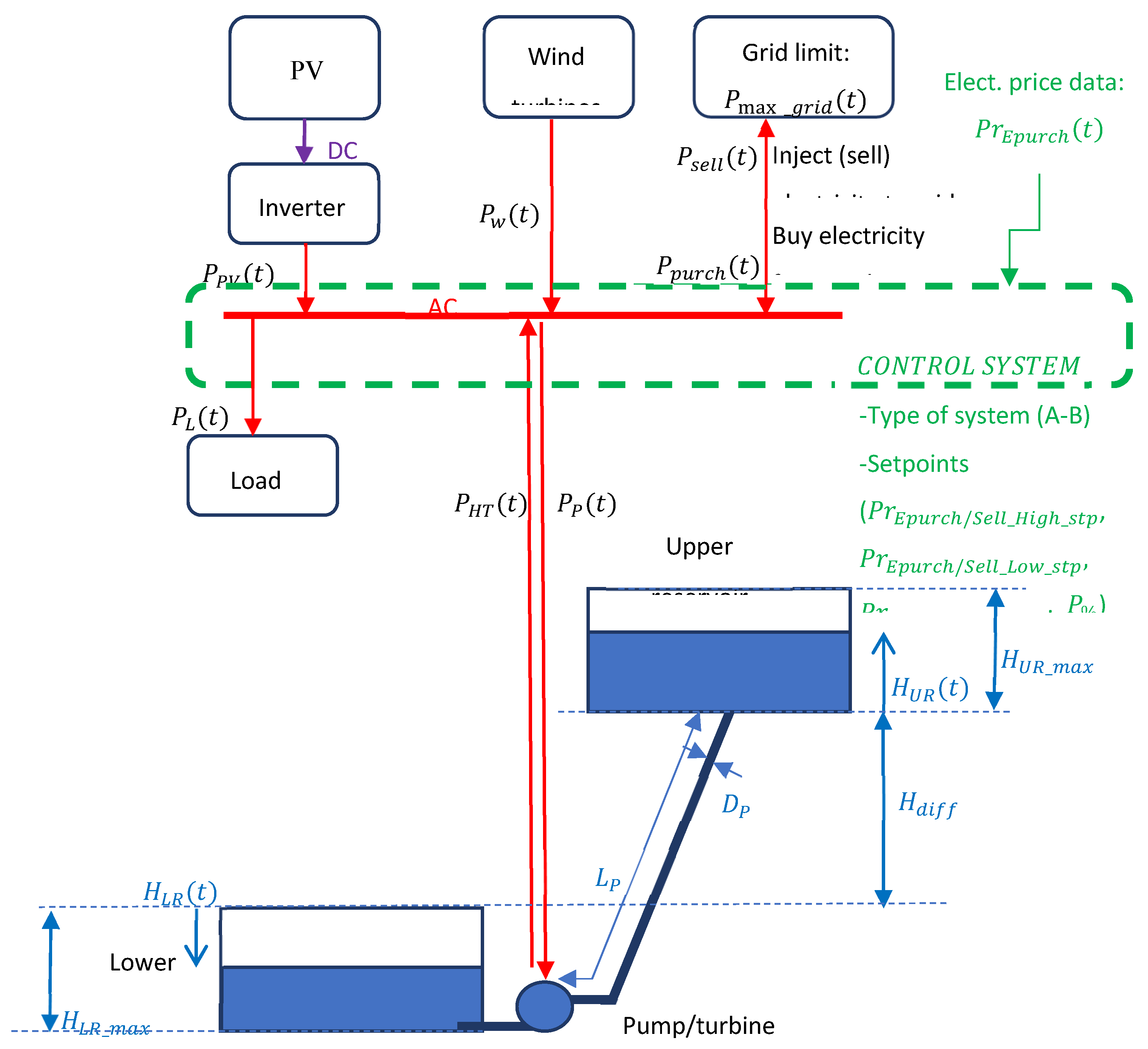
Figure 2.
Wind turbine output curve of a 500-kW wind turbine with pitch control. Standard (green curve) and other conditions (dotted red curve).
Figure 2.
Wind turbine output curve of a 500-kW wind turbine with pitch control. Standard (green curve) and other conditions (dotted red curve).
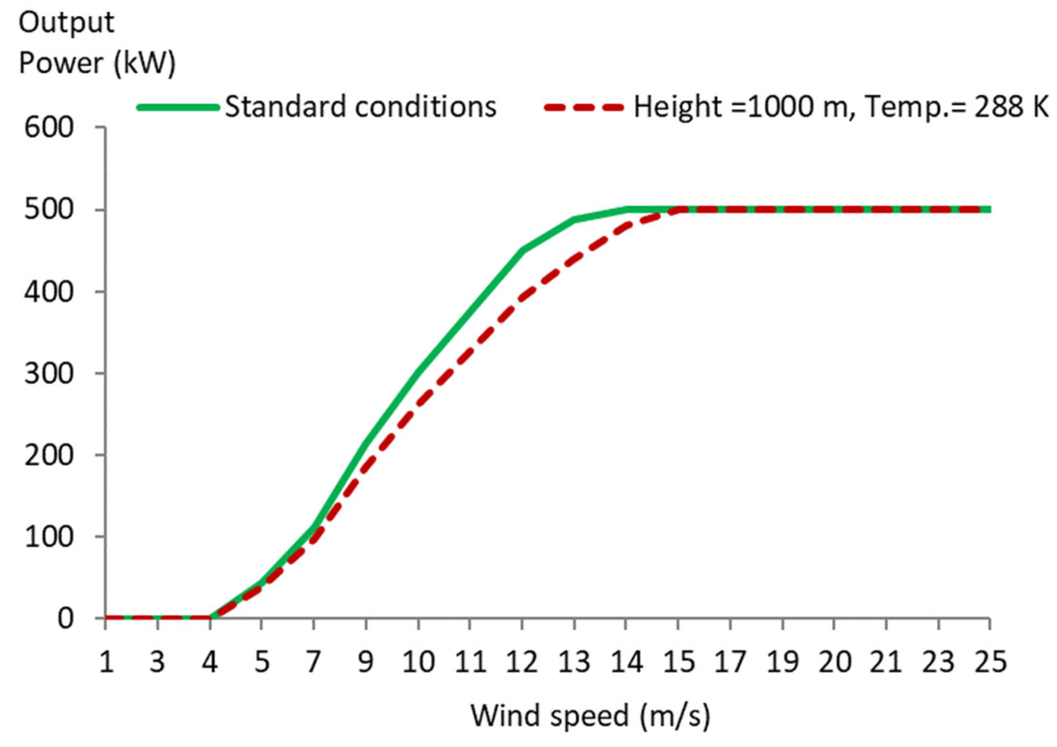
Figure 3.
Efficiency (%) vs. maximum flow (%) of the pump-turbine reversible machine considered in this study.
Figure 3.
Efficiency (%) vs. maximum flow (%) of the pump-turbine reversible machine considered in this study.
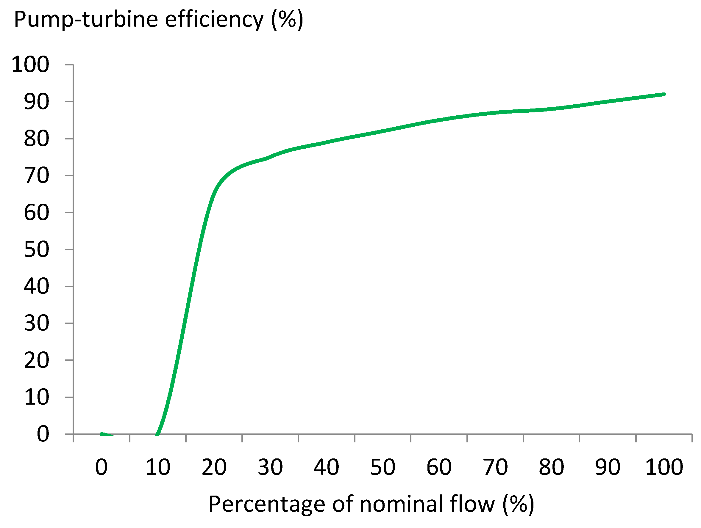
Figure 4.
Annual load consumption during the years.
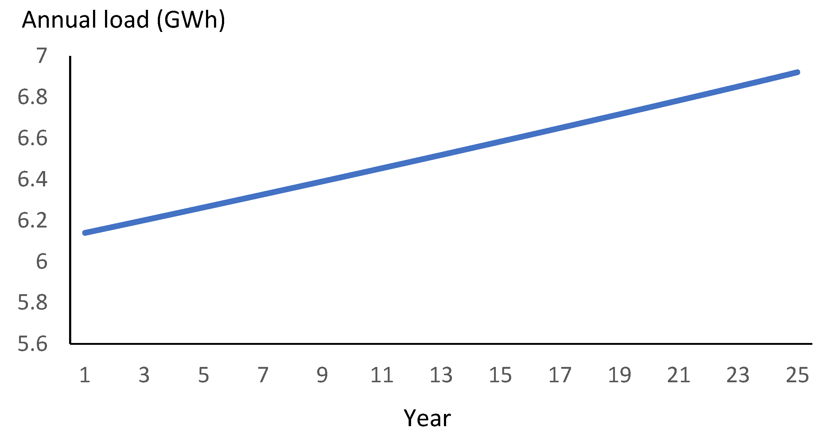
Figure 5.
Annual energy (GWh/year) supplied by the different components, unmet load, and sell energy during the 25 years of the simulation.
Figure 5.
Annual energy (GWh/year) supplied by the different components, unmet load, and sell energy during the 25 years of the simulation.
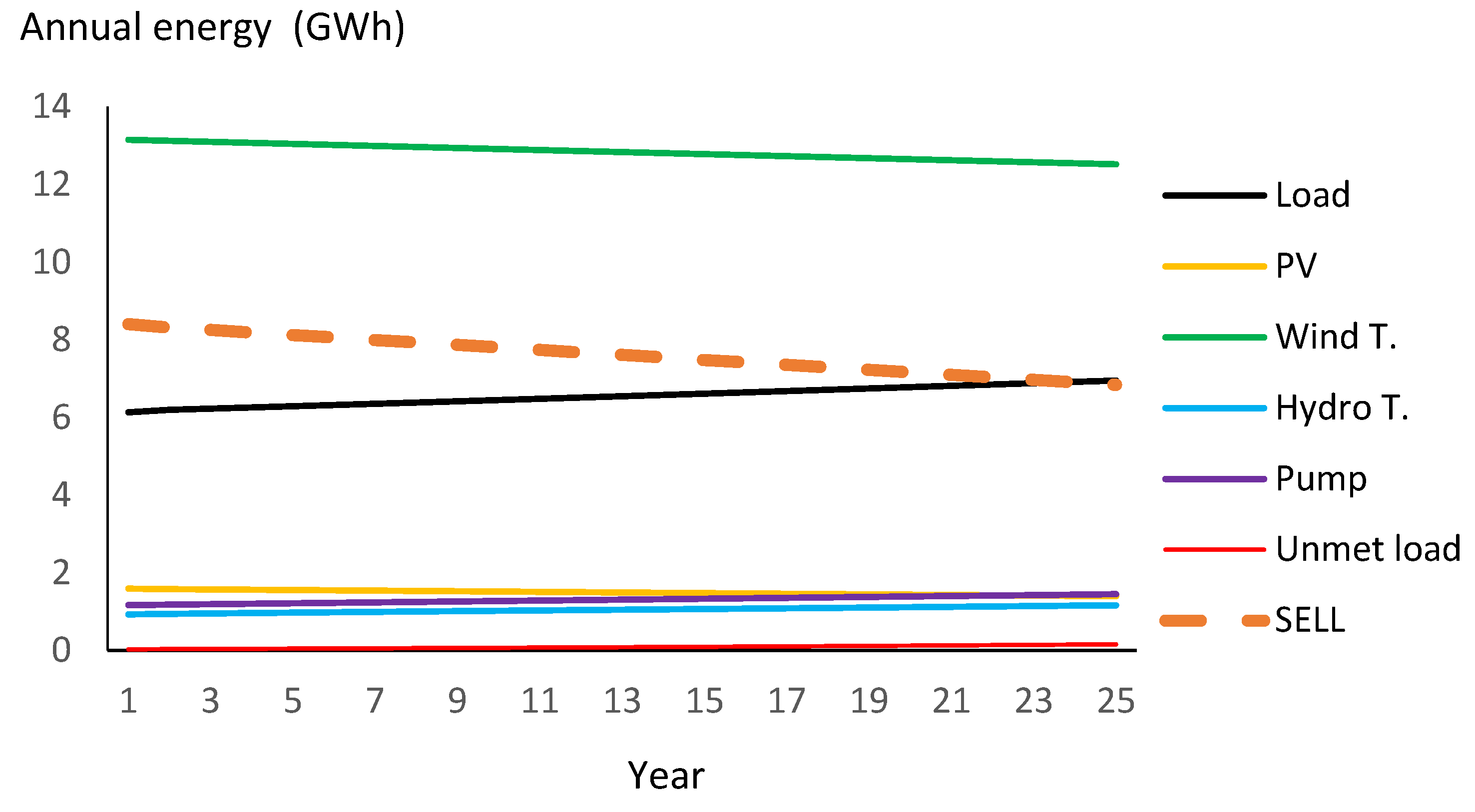
Figure 6.
Hourly irradiance (W/m2) in Zaragoza (slope of 35° and azimuth of 0°).
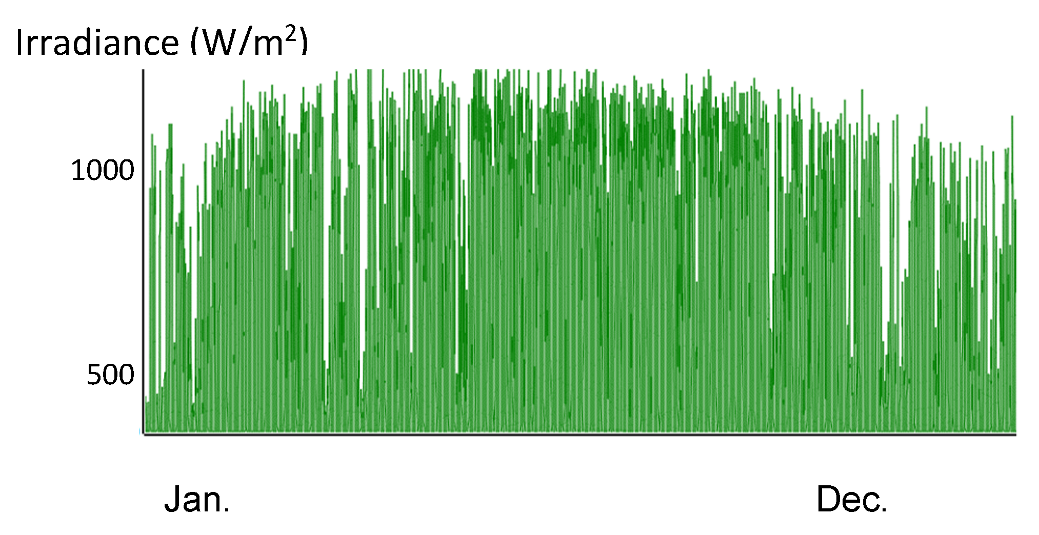
Figure 7.
Annual irradiation variation over the average (%).
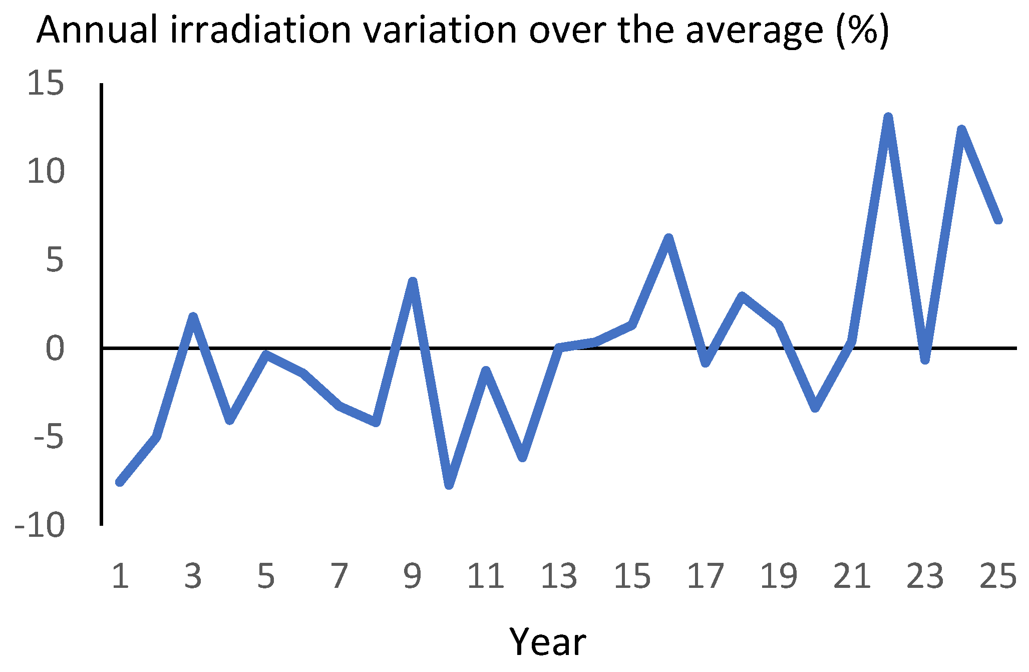
Figure 8.
Hourly wind speed (m/s) at a height of 53 m in Zaragoza.
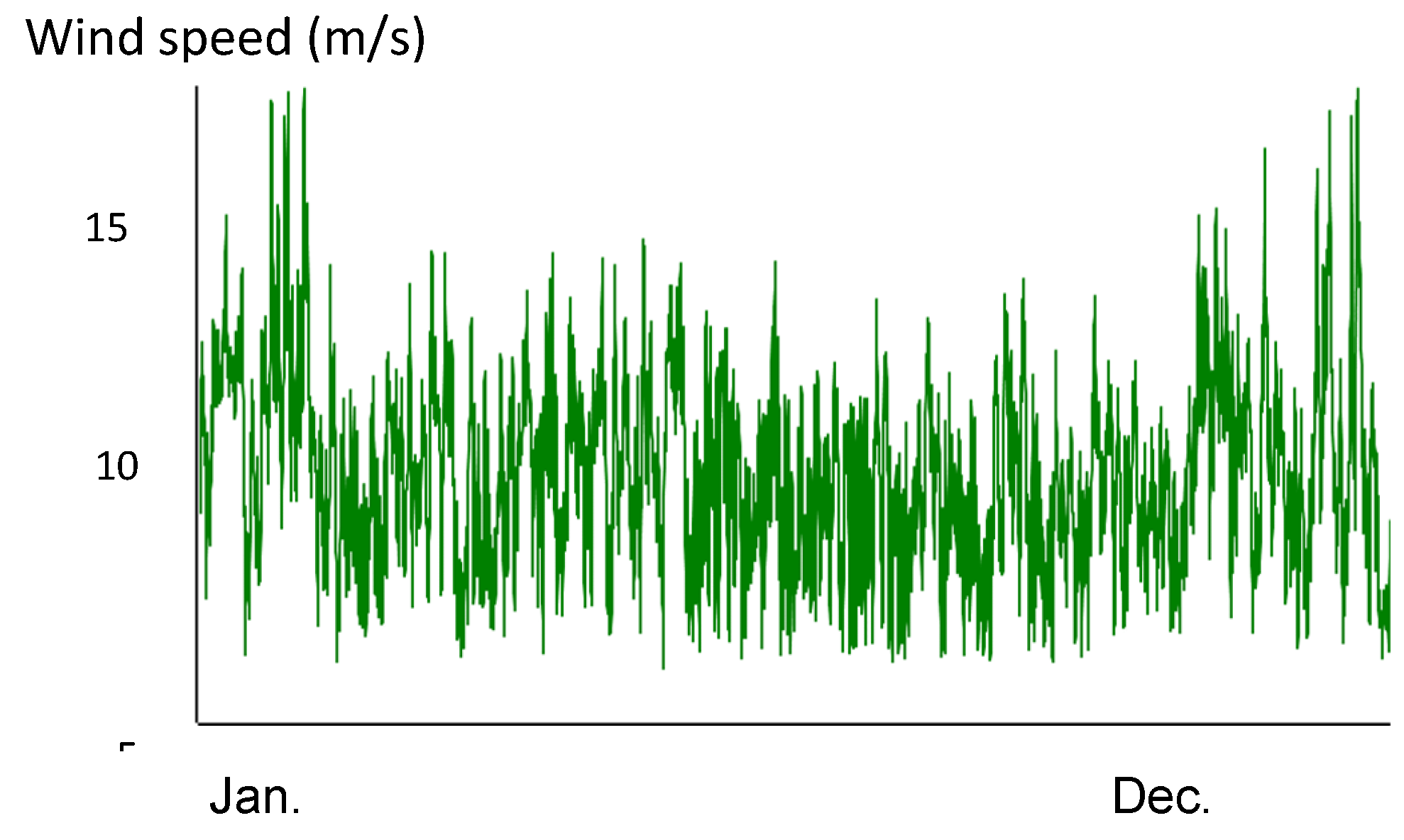
Figure 9.
Annual wind speed variation over the average (%).
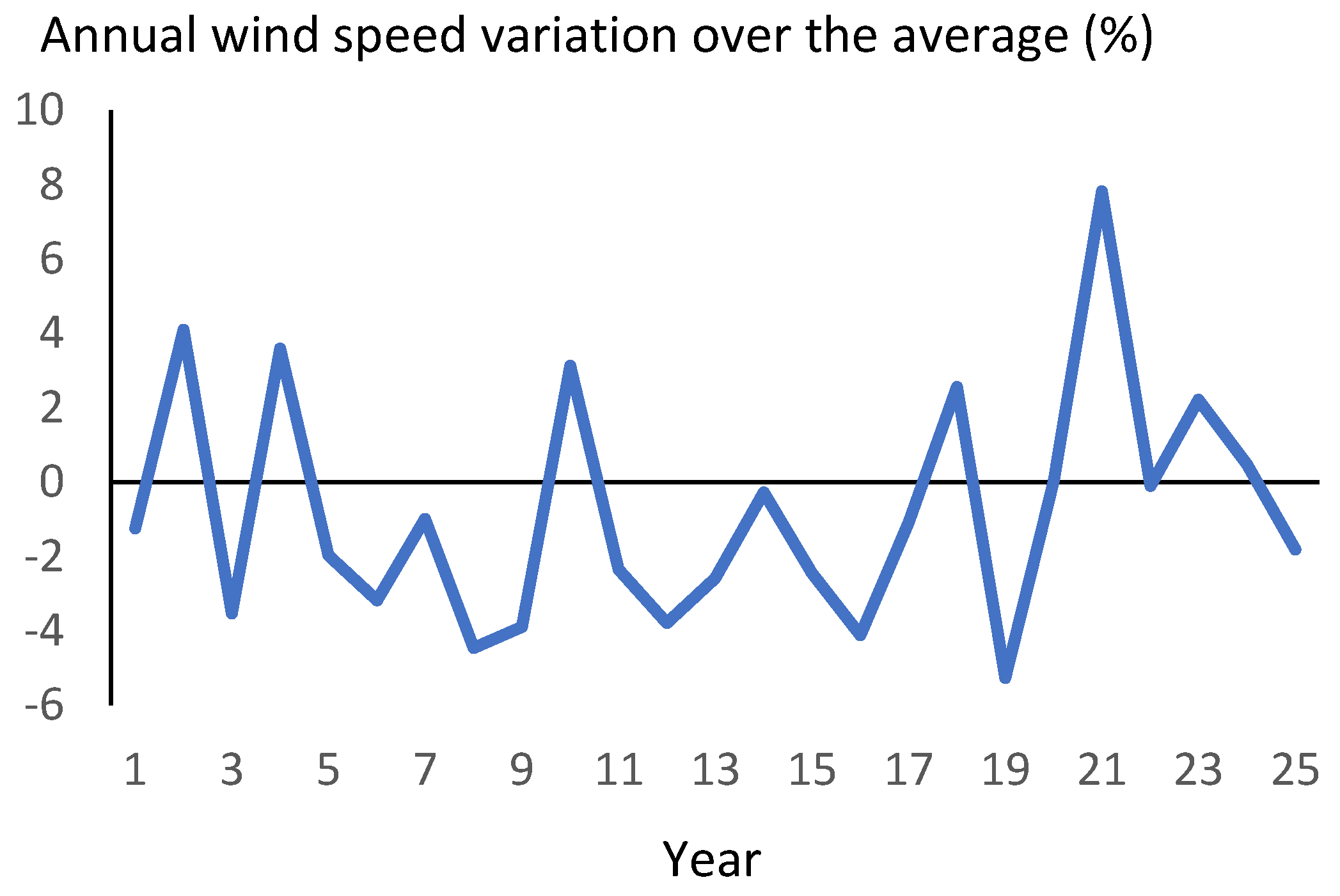
Figure 10.
Hourly sell electricity price for the first year.
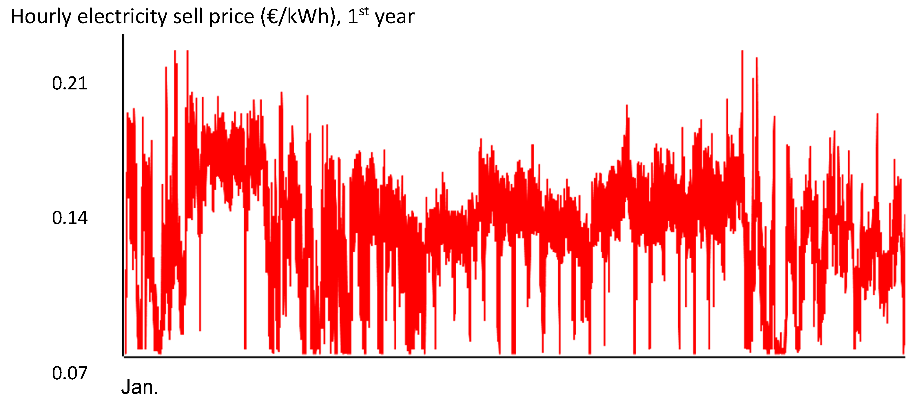
Figure 11.
Daily maximum minus minimum sell price difference (€/kWh) for the first year.
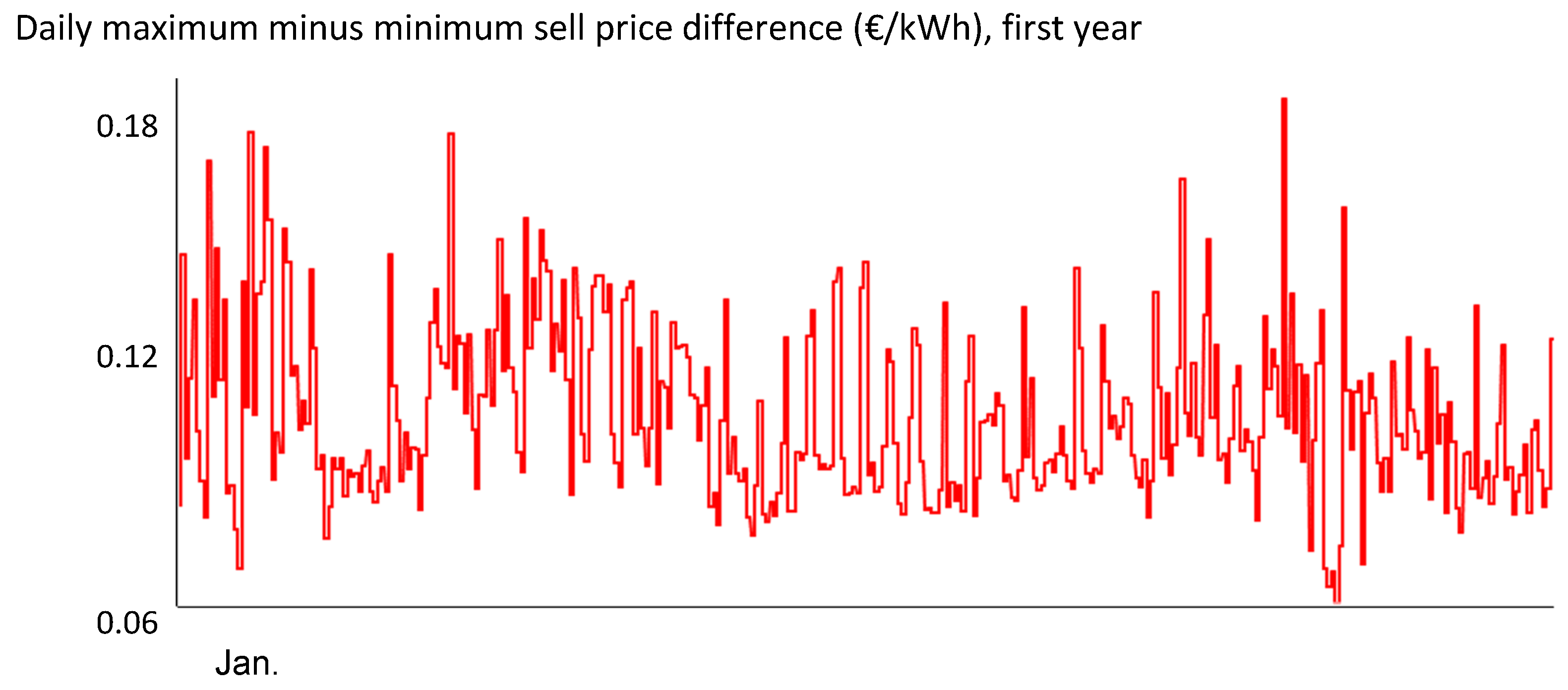
Figure 12.
Probability density function of the daily maximum minus minimum sell price difference (€/kWh) for the first year.
Figure 12.
Probability density function of the daily maximum minus minimum sell price difference (€/kWh) for the first year.
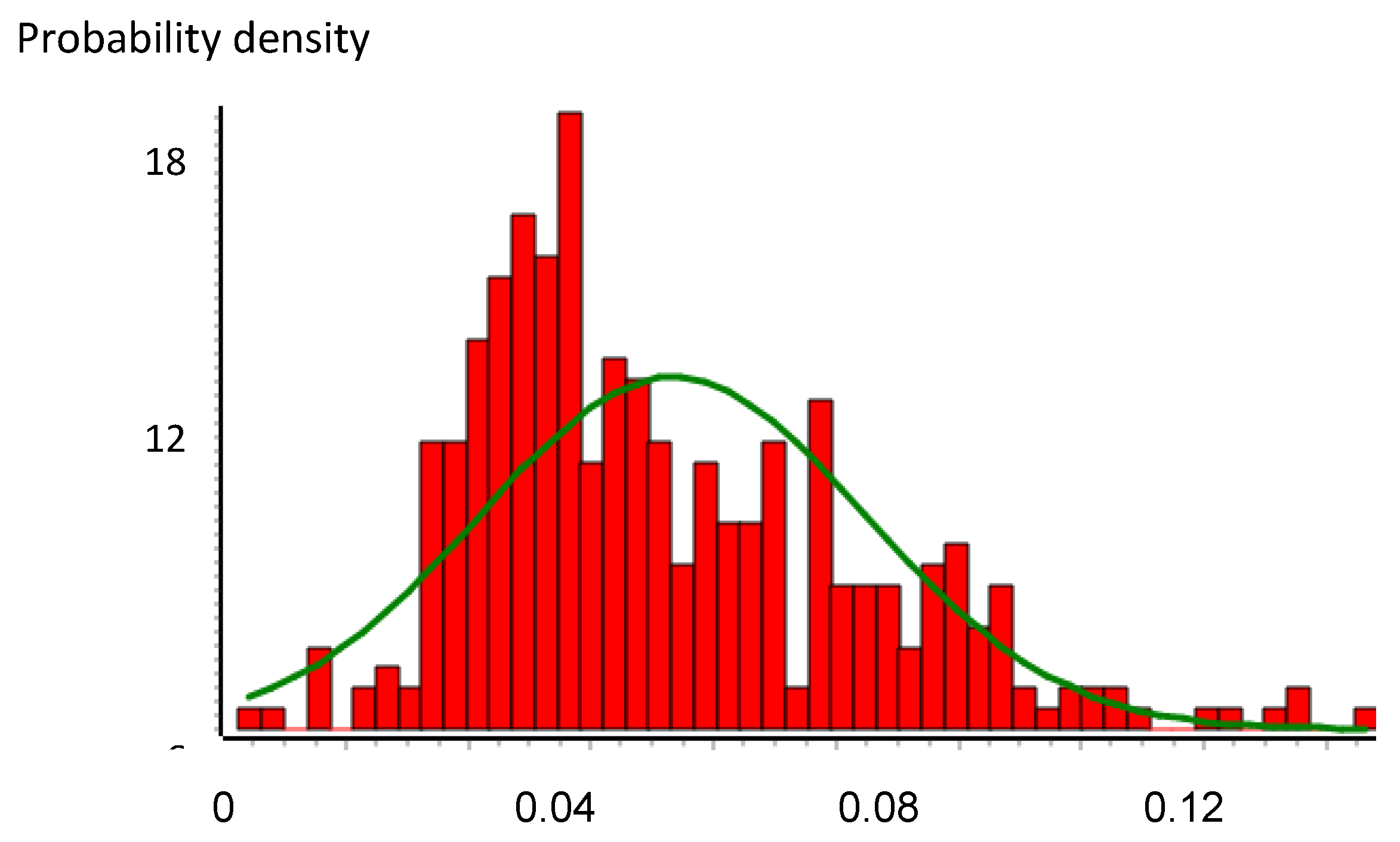
Figure 13.
Annual and cumulated inflation for the electricity price (%).
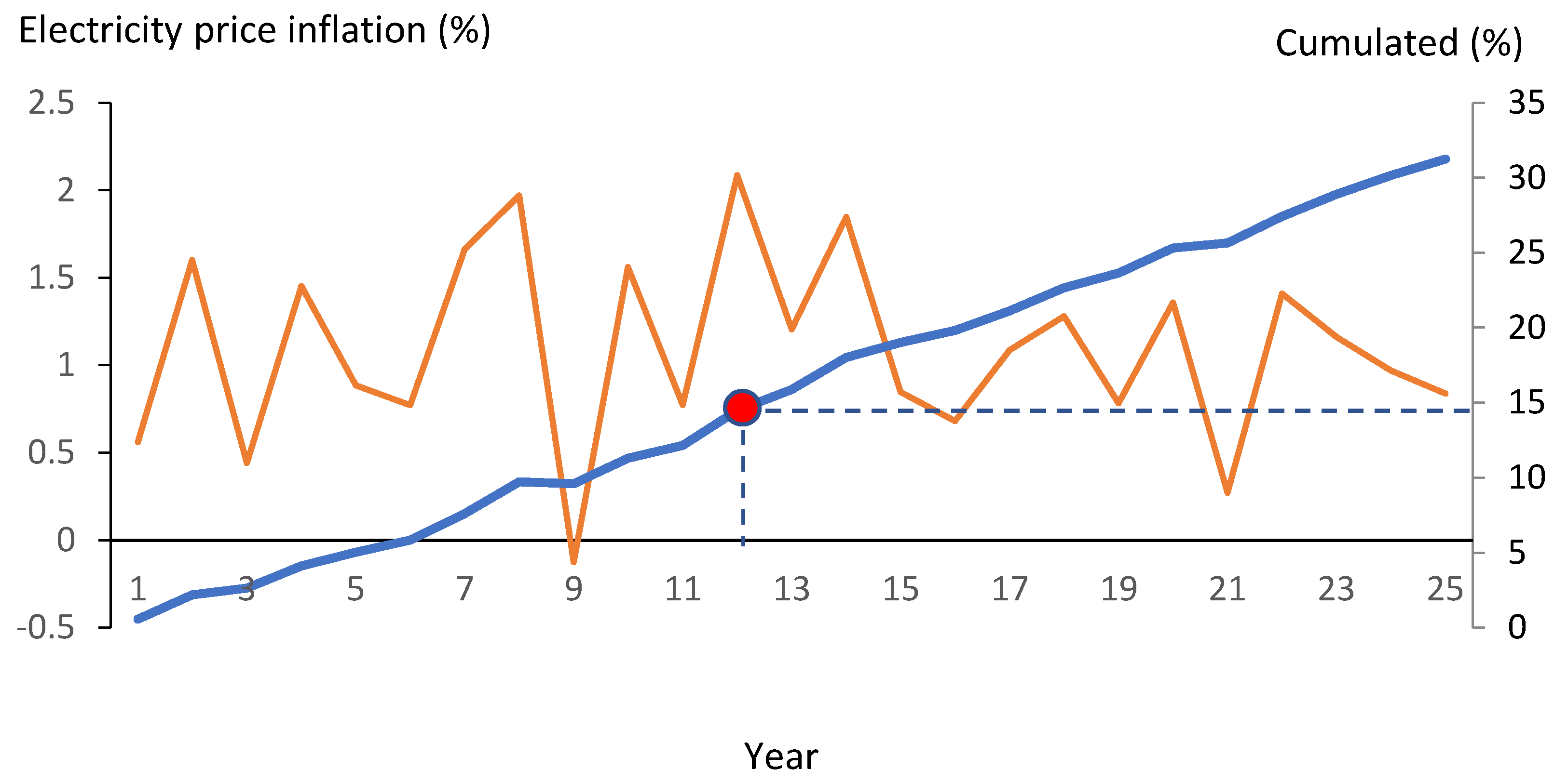
Figure 14.
Daily average hourly electricity sell price for the different years, all referred to the beginning of the system (year 0) (€/kWh).
Figure 14.
Daily average hourly electricity sell price for the different years, all referred to the beginning of the system (year 0) (€/kWh).
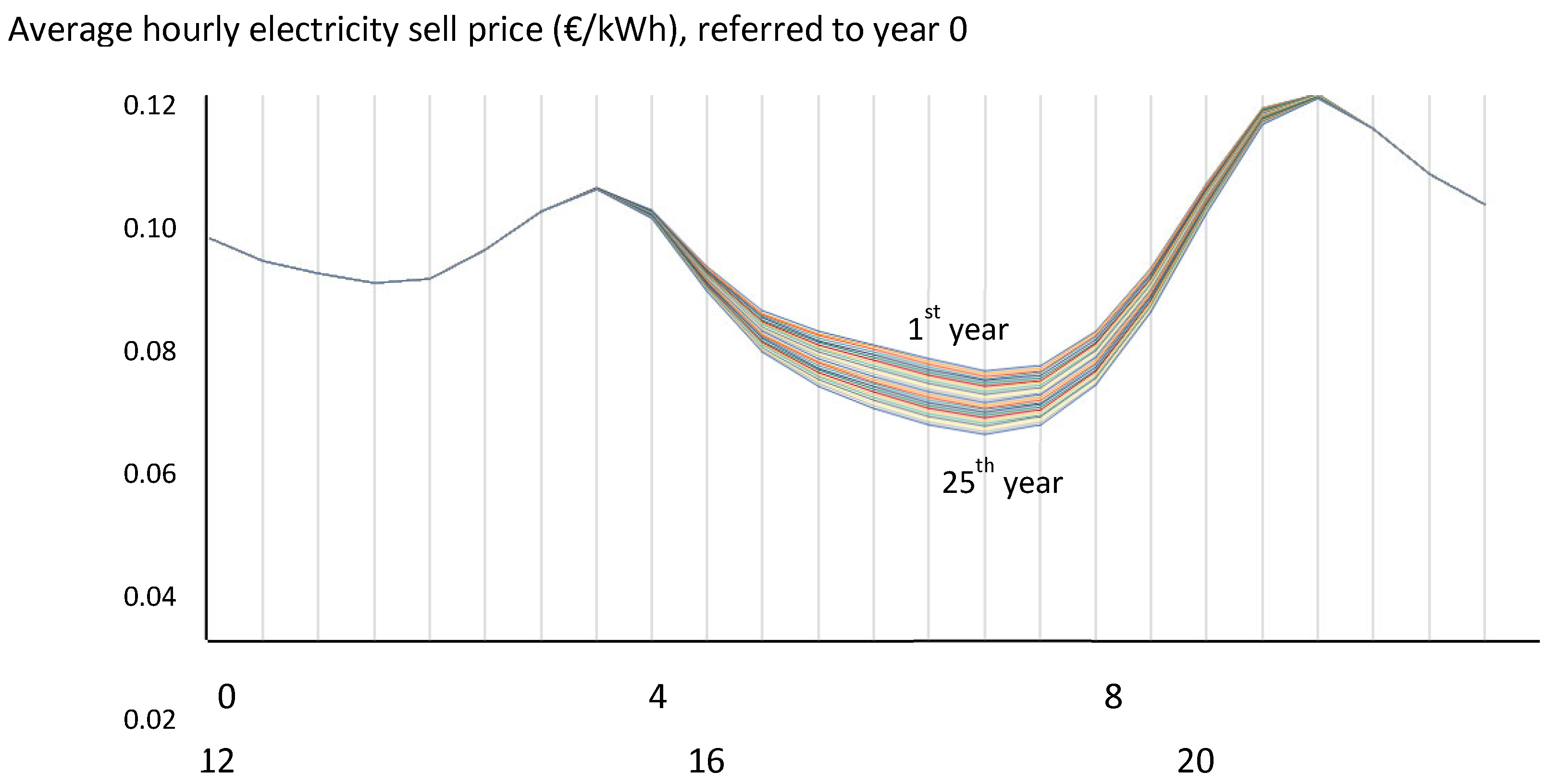
Figure 15.
PV Inverter efficiency.
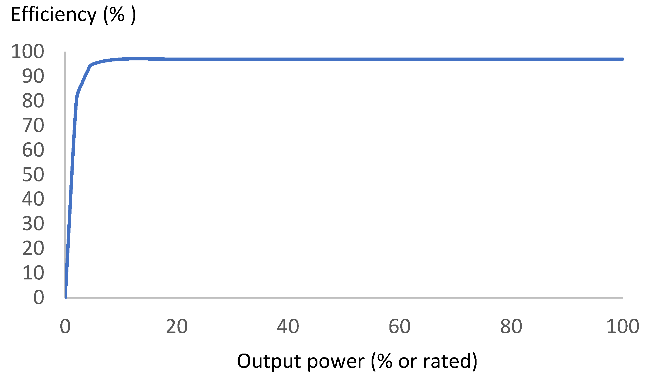
Figure 16.
Evolution of the NPC of the best system found for each generation of the GA.
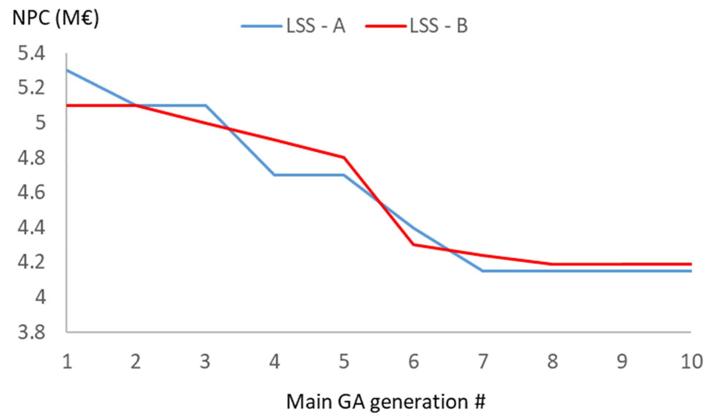
Figure 17.
Simulation of two consecutive days, March 9 and 10, year 12. LSS optimal system without PHS.
Figure 17.
Simulation of two consecutive days, March 9 and 10, year 12. LSS optimal system without PHS.
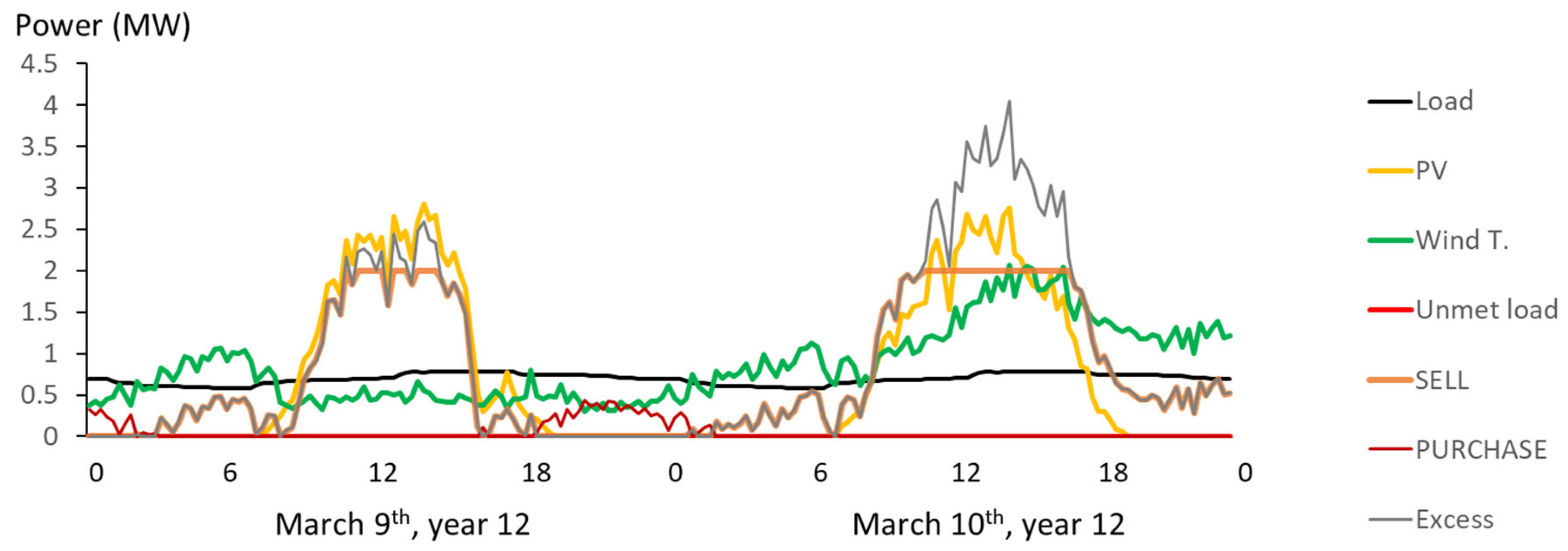
Figure 18.
Annual energy, LSS optimal system without PHS.
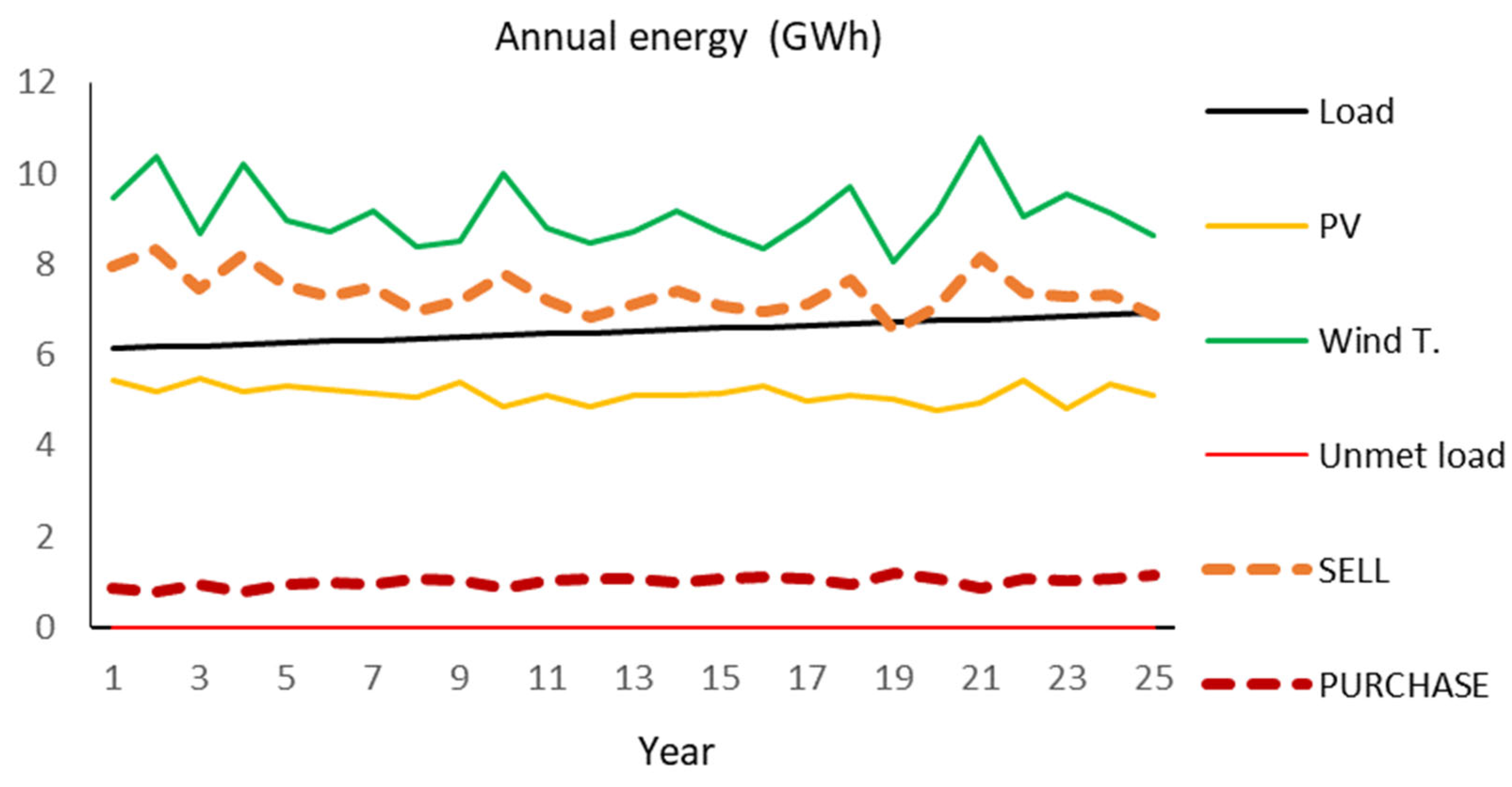
Figure 19.
Simulation of two consecutive days, March 9–10, year 12. LSS optimal system with PHS, type A project.
Figure 19.
Simulation of two consecutive days, March 9–10, year 12. LSS optimal system with PHS, type A project.
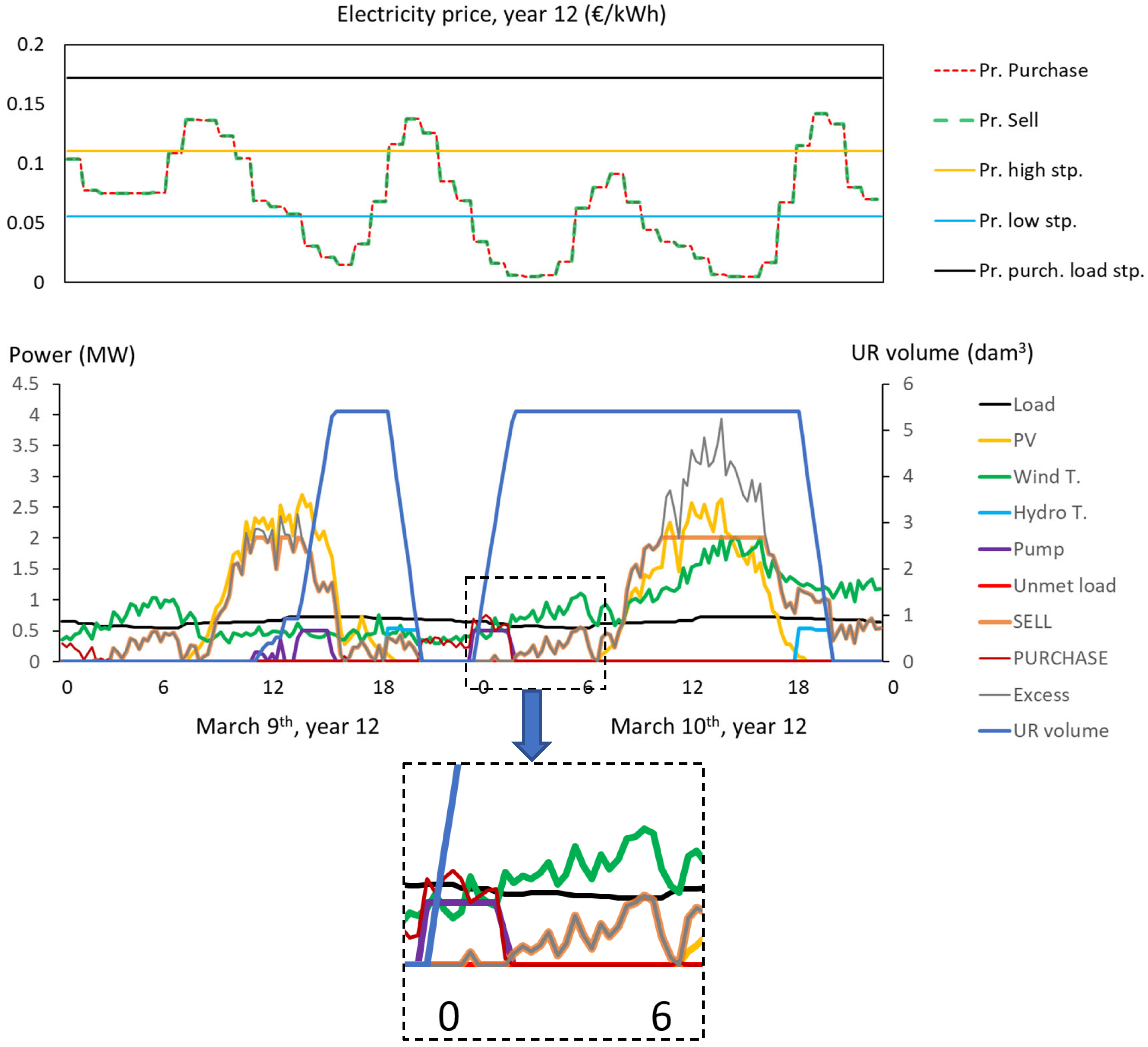
Figure 20.
Simulation of year 12. LSS optimal system with PHS, type A project.
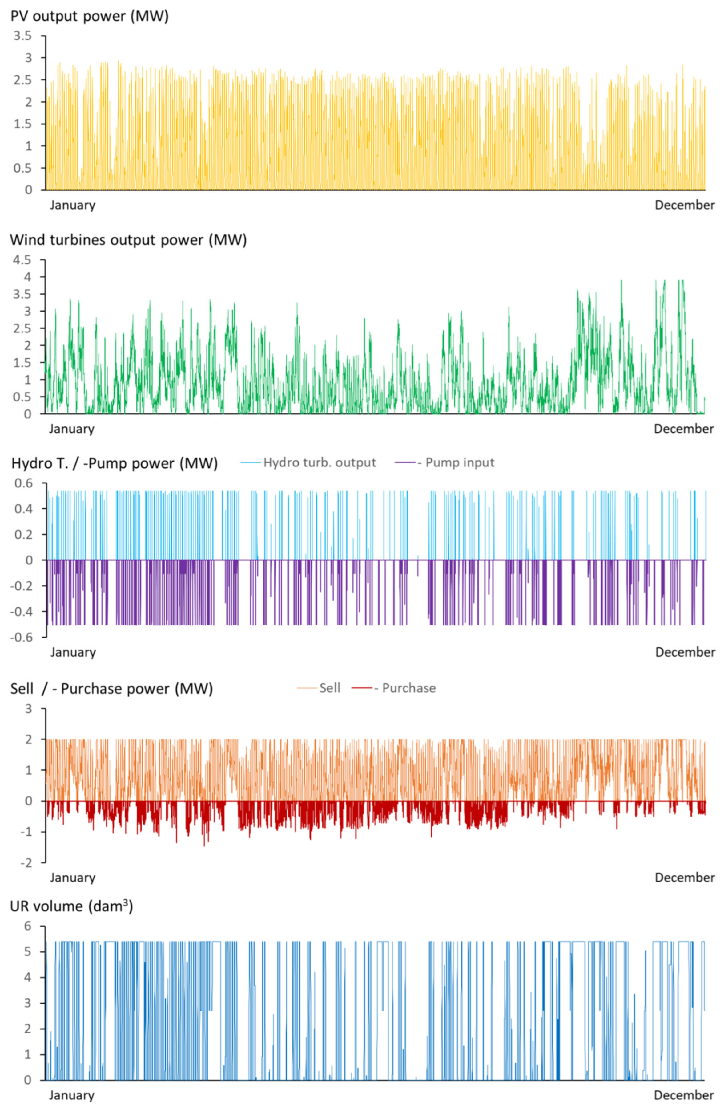
Figure 21.
Annual energy, LSS optimal system with PHS, type A project.
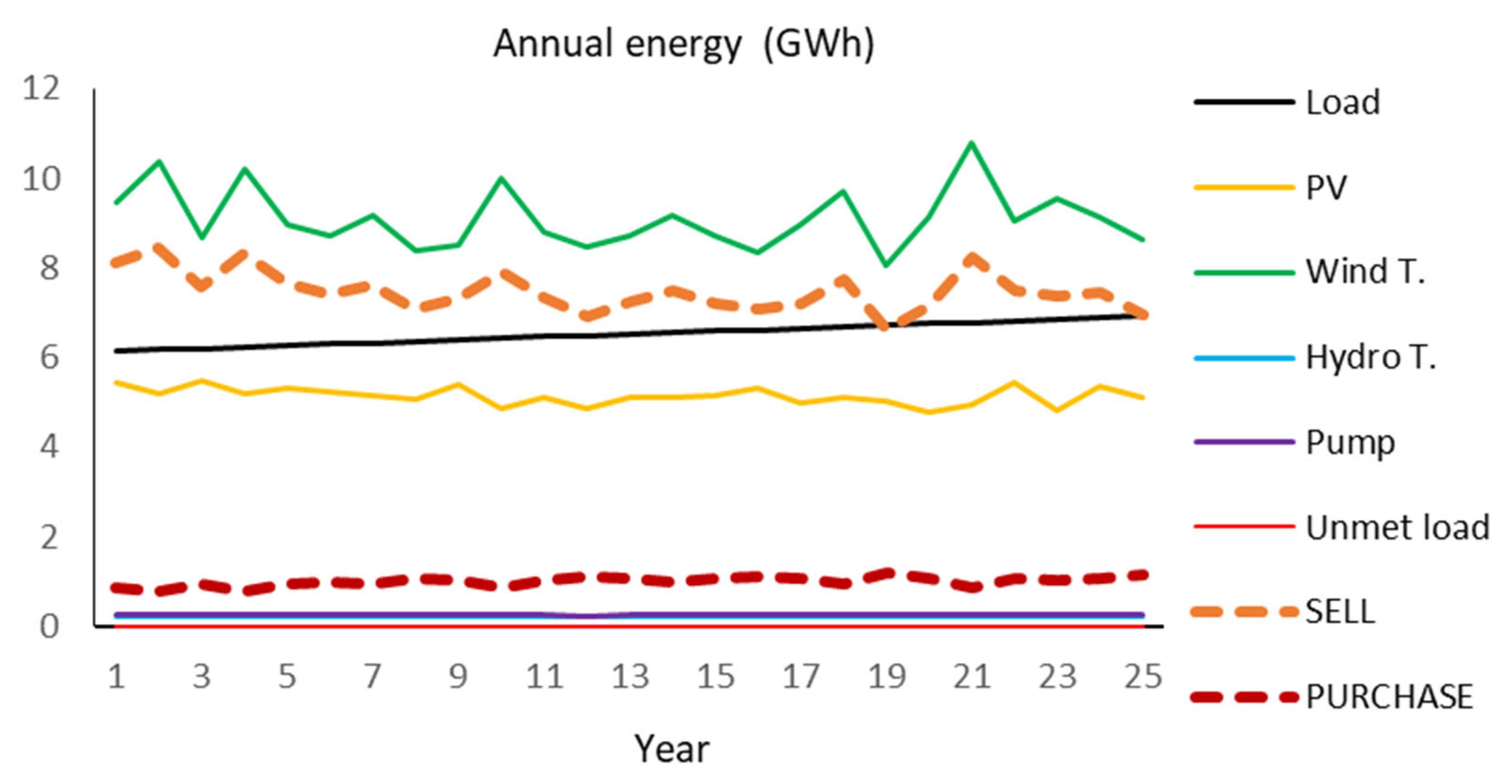
Figure 22.
Simulation of two consecutive days, March 9–10, year 12. LSS Optimal system with PHS, type B project.
Figure 22.
Simulation of two consecutive days, March 9–10, year 12. LSS Optimal system with PHS, type B project.
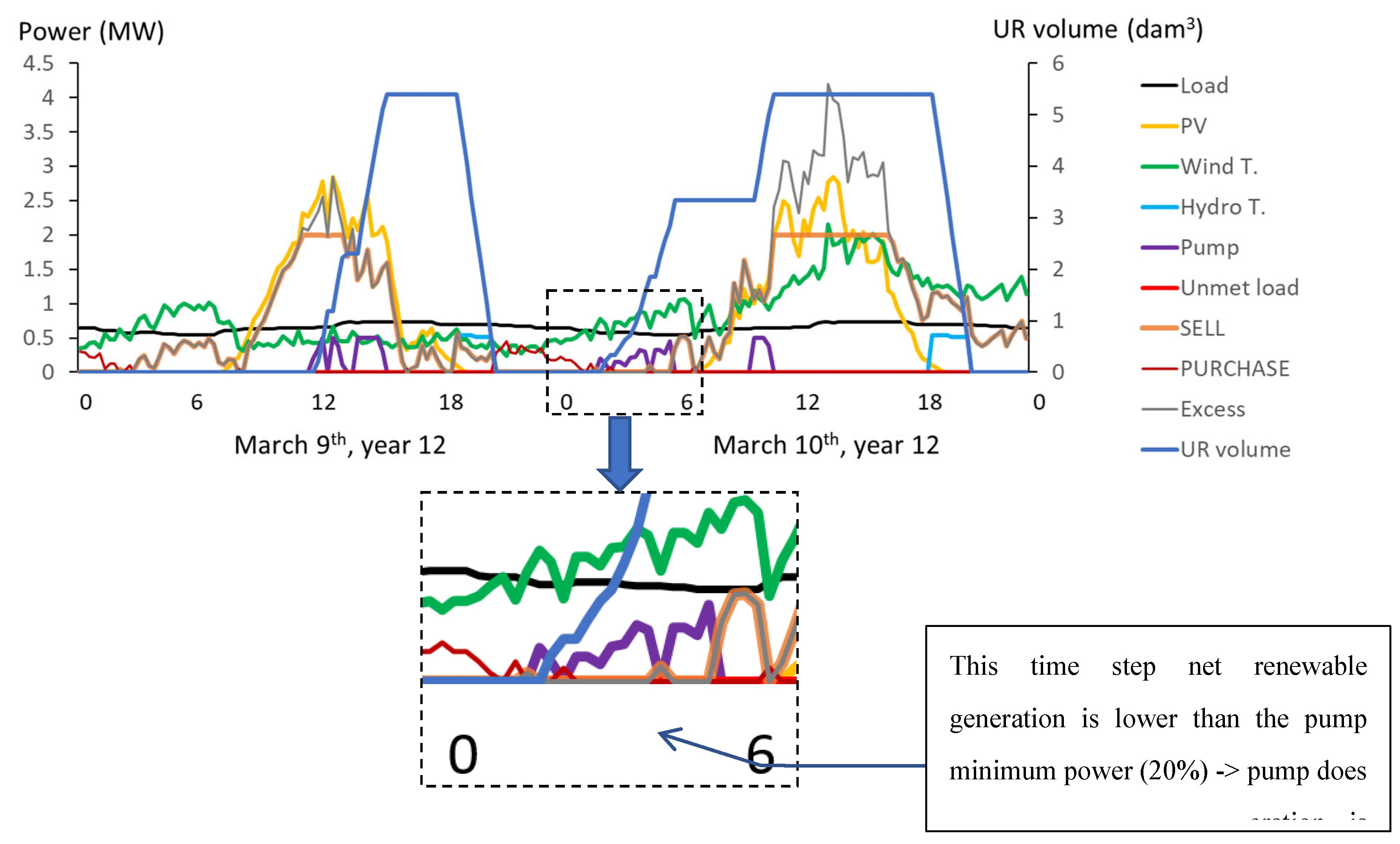
Figure 23.
Optimal systems found for the different locations: LSS systems.
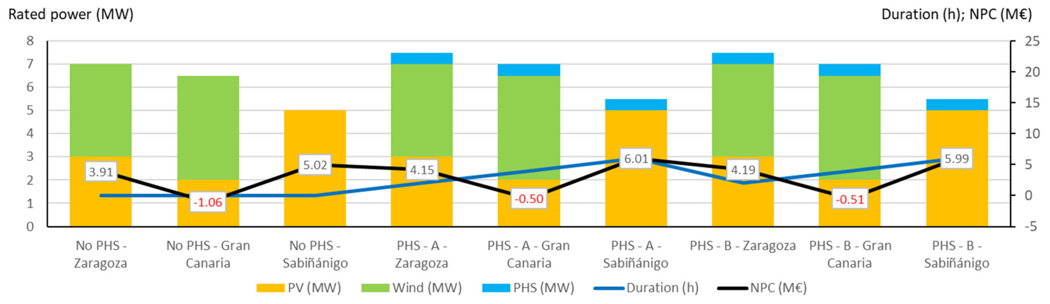
Figure 24.
Optimal systems found for the different locations: PGS systems.
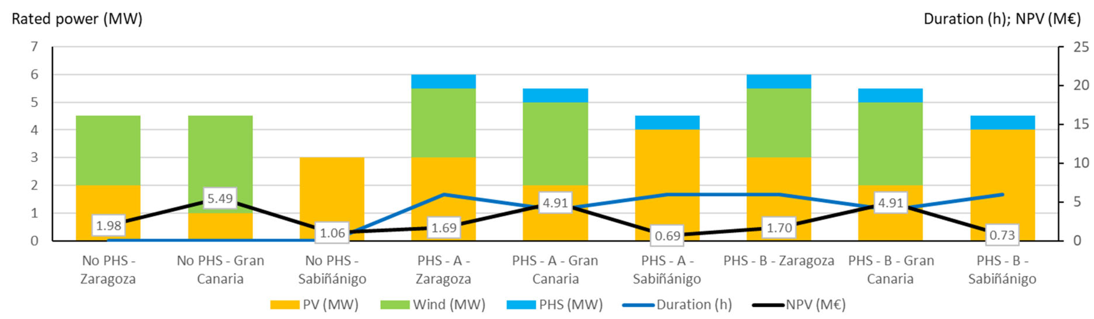
Figure 25.
Hourly sell electricity price of first year. Hypothetical electricity price.
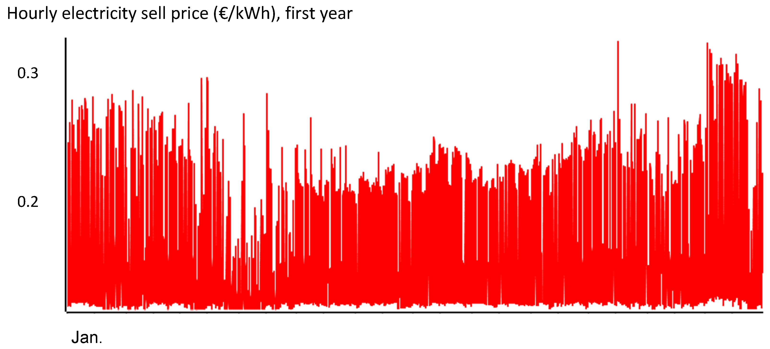
Figure 26.
Daily maximum minus minimum sell price difference (€/kWh), first year. Hypothetical electricity price.
Figure 26.
Daily maximum minus minimum sell price difference (€/kWh), first year. Hypothetical electricity price.
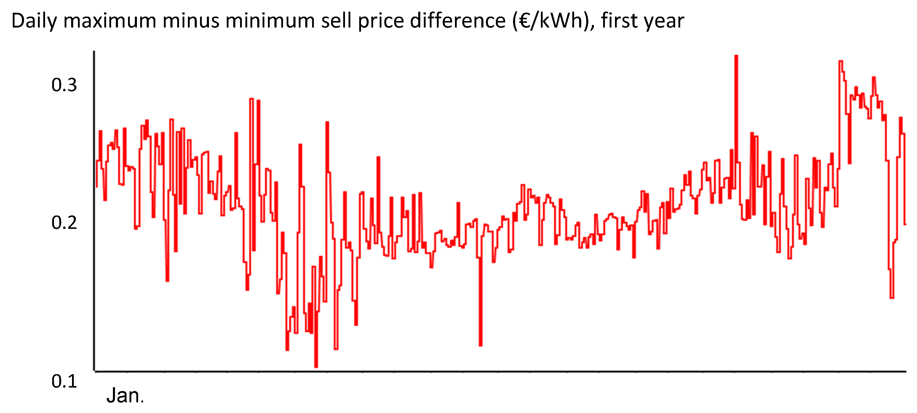
Figure 27.
Probability density of the daily maximum minus minimum sell price difference (€/kWh), first year. Hypothetical electricity price.
Figure 27.
Probability density of the daily maximum minus minimum sell price difference (€/kWh), first year. Hypothetical electricity price.
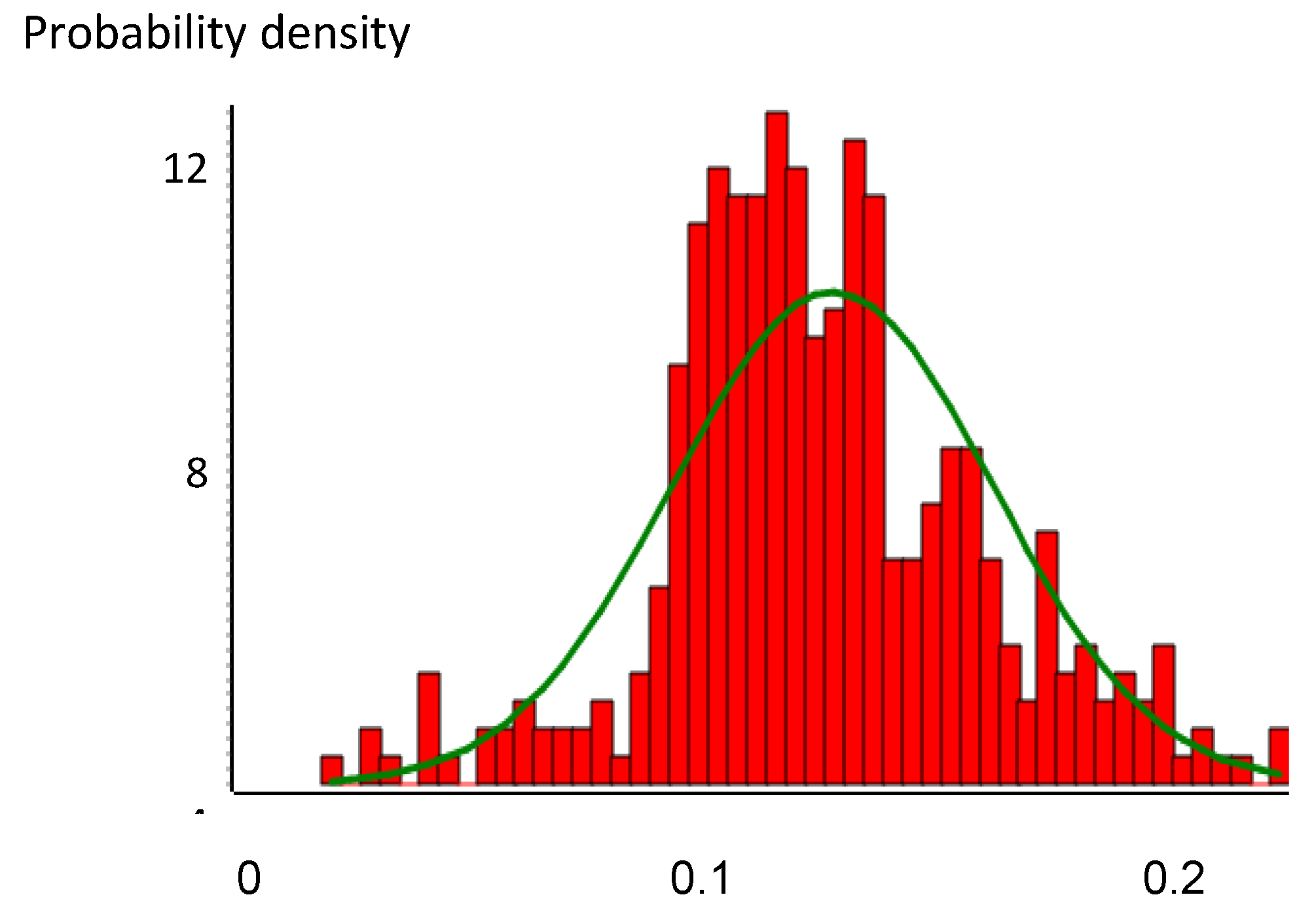
Figure 28.
Daily average hourly electricity price, referred to year 0. Hypothetical electricity price.
Figure 28.
Daily average hourly electricity price, referred to year 0. Hypothetical electricity price.
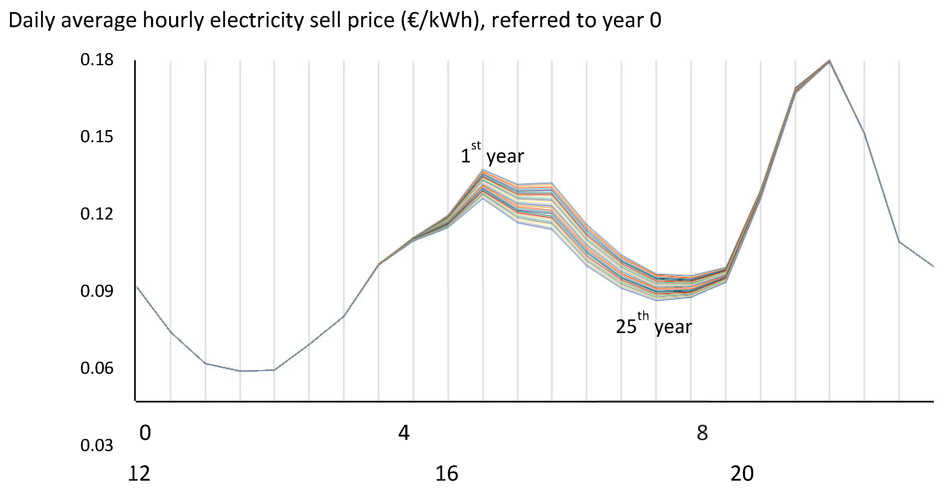
Figure 29.
Optimal systems found for the different RTP electrical price: LSS system.
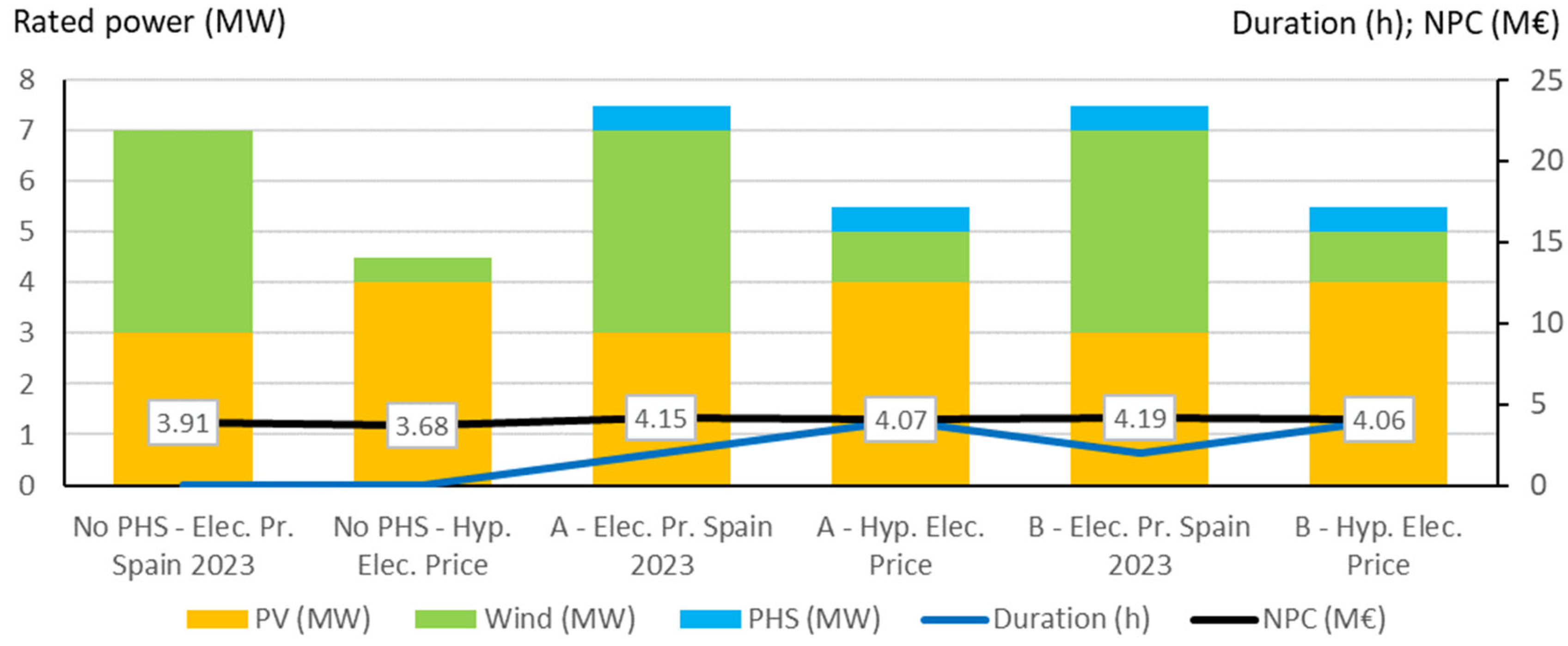
Figure 30.
Optimal systems found for the different RTP electrical price: PGS system.

Figure 31.
Optimal systems found for the different PHS CAPEX: LSS system.
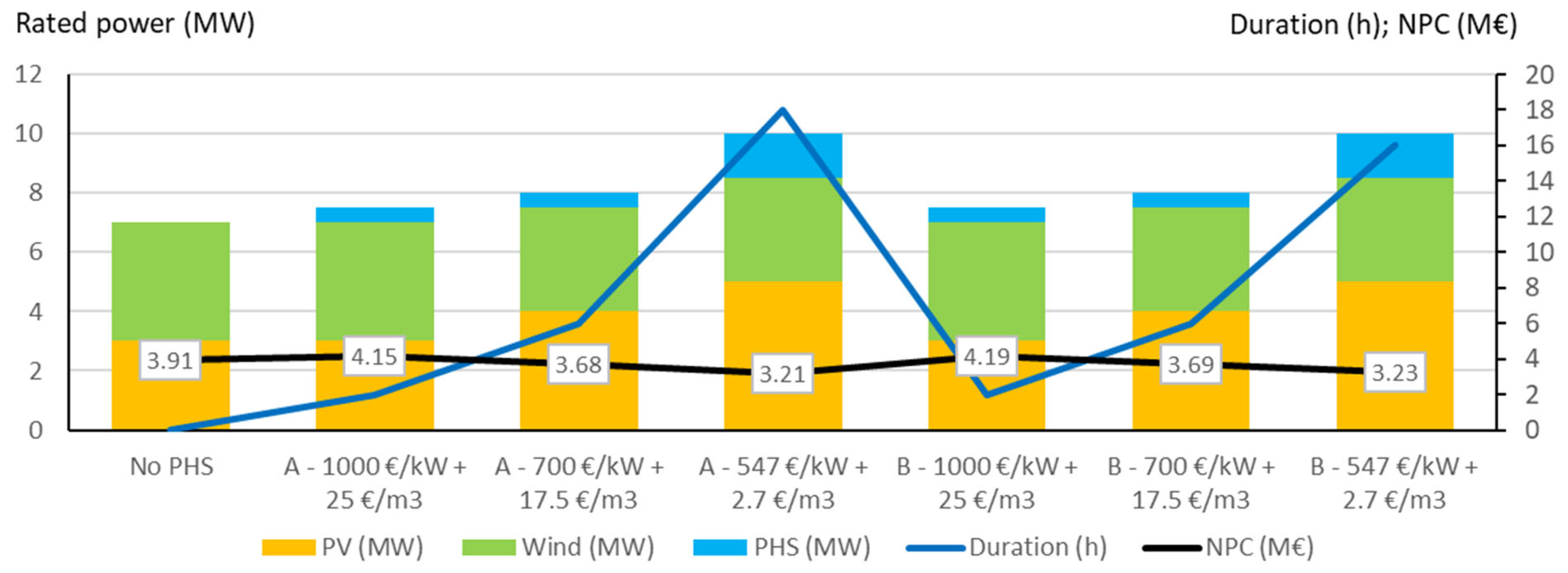
Figure 32.
Optimal systems found for the different PHS CAPEX: PGS system.
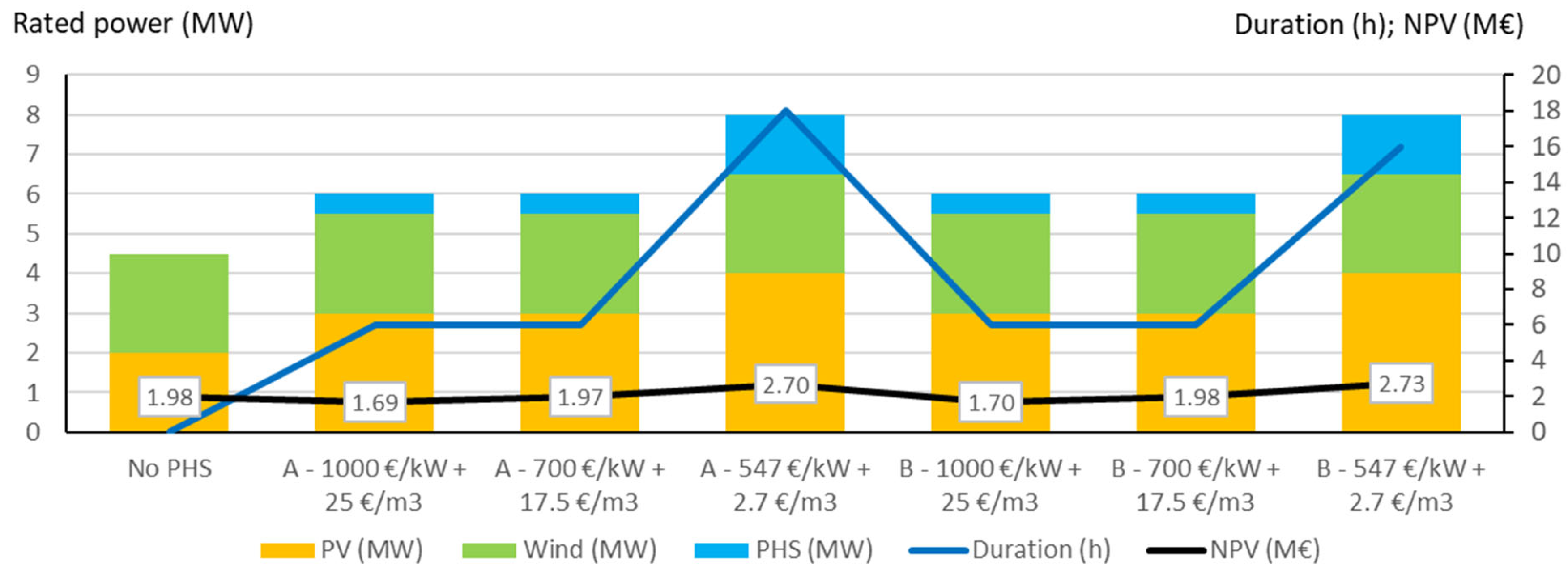

Table 1.
Performance of the two different types of projects (A or B) of PV-wind-PHS systems.
| Type A: Allowed to buy energy for arbitrage | Type B: Not allowed to buy energy for arbitrage | |
|---|---|---|
| Allowed to purchase electricity from the grid for arbitrage (for pumping) | ✓ | ✗ |
| Arbitrage sell electricity price set points ) | ✕ | ✓ |
| Arbitrage purchase electricity price set points () | ✓ | ✕ |
| Operation principle: During each time step t: | ||
| - If there is net renewable generation () or no load and no generation. | - If buy electricity price is higher than the set point () → Energy arbitrage (discharge): Priority is injecting (sell) electricity to the grid (net renewable generation + hydro t. max. power*): - If → Energy arbitrage (charge): Priority pumping water with a renewable surplus power; if it is lower than pump rated power, buy electricity to run the pump at the rated power: - If → No arbitrage: Priority is injecting the net renewable generation to the grid. |
-If buy electricity price is higher than the set point ( → Energy arbitrage (discharge): Priority is injecting (sell) electricity to the grid (net renewable generation + hydro turbine max. power*): - If → Energy arbitrage (charge): Priority is pumping water with renewable surplus power: - If → No arbitrage: Priority is injecting the net renewable generation to the grid: |
| - If there is net load () | If > . . Further, consider priorities for energy arbitrage (depending on the electricity price) shown above |
|
* PHT_max(t) represents the maximum available power that can be supplied by the hydro turbine at time t, considering its rated power, rated flow, and water volume in the reservoirs (detailed in Section 2.1.4).
Table 2.
Results of the optimal system obtained by Nassar et al. [28] and comparison with this work.
Table 2.
Results of the optimal system obtained by Nassar et al. [28] and comparison with this work.
| Total renewable generation (GWh/year) | Energy injected to the grid (%) | Direct supply to the load from renewable sources (%) | Demand covered by hydro turbine (%) | Unmet load (%) | |
| Nassar et al.’s optimal system (lowest LCOE) [28] | 14.6 | 57.1 | 85 | 15 | 0 |
| This work, assuming the same inputs as Nassar et al. [28], simulating their optimal system (with several assumptions) | 14.72 | 57.6 | 84.6 | 15.4 | 0.4 |
| This work, same inputs as Nassar et al. [28] plus a variable head, pump-turbine variable efficiencies, and simulating 25 years. | 14.33 av. 13.92 min. 14.74 max. |
53.08 av. 49.17 min. 57.01 max. |
83.92 av. 83.19 min. 84.77 max. |
16.6 av. 15.22 min. 16.81 max. |
1.41 av. 0.61 min. 2.35 max. |
Table 3.
Main characteristics of the system.
| Variable | Value |
| Location | Zaragoza (Spain) (41.66°N, 0.88°W) |
| System lifetime | 25 years |
| Electrical load (First year) | 1.2 MW peak power, 6.14 GWh annual load (Nassar et al. [28], Section 3.1). |
| Annual increase in electrical load | 0.5% |
| Unmet load allowed | 0%. |
| Maximum grid power | 2 MW |
| Nominal discount rate | 8% |
| General inflation | 2% |
| Sell and purchase electricity Price | RTP (First year market price Spain 2023) |
| Access charge | 0.02 €/kWh fixed. |
| 0.3 | |
| 0 | |
| Mean of electricity price inflation | 1% |
| Standard deviation of electricity price inflation | 0.5% |
|
PV: |
|
| CAPEX | 0.855 €/Wac [50] |
| OPEX | 0.5% of CAPEX per year [51] |
| Nominal power (AC) | 0 to 5 MWac, steps of 1 MWac |
| Slope and azimuth | 35° and 0°. |
| Lifetime | 25 years |
| 0.5% [44] | |
| 43 °C | |
| 95% | |
| −0.41%/°C | |
| PV inverter DC/AC ratio | 1.25 |
| Inverter efficiency | Figure 15 [52] |
|
Wind turbines: |
|
| CAPEX | 1.3 €/W [53] |
| OPEX | 2% of CAPEX per year[53] |
| Nominal power | 500 kW |
| Number in parallel | 0−10 |
| Lifetime | 25 years |
| Hub height | 53 m |
| Roughness | 0.1 m |
| 0.2 [37] | |
| 98% | |
| Power curve | Figure 2 |
|
PHS: |
|
| Pump/turbine reversible machine CAPEX (inc. civil works) | 1,000 €/kW |
| Pump/turbine OPEX | 1.5% of CAPEX per year + 0.35 €/kWh |
| Reservoirs CAPEX | 25 €/m3 (130 €/kWh considering 70 m head) |
| Lifetime | 50 years |
| Pump/turbine start-up costs | 0.1 €/MW [31] |
| Nominal power | 0.5–2.5 MW, steps of 0.5 MW |
| Nominal flow | 0.75–3.75 m3/s, steps of 0.75 m3/s |
| Efficiency curve | Figure 3 |
| Pump minimum input power | 20% of nominal power |
| Head | 70 m |
| Upper reservoir duration: (h) | 2–20 h, steps of 2 h |
| 100% | |
| 0% | |
| Lifetime | 25 years |
| 0.6 m < Dp < 1.5 m. Calculated for each case to obtain a water speed of 2.5 m/s for nominal turbine flow. | |
| 250 m | |
| 0.8 | |
| 0.05 mm | |
| 70 m | |
| 5 m |
Table 4.
Results of the different optimisations with the LSS system.
| Project type | LSS - Optimal system without PHS | LSS - A (buy for arbitrage) - Optimal with PHS |
LSS - B (no buy for arbitrage) - Optimal with PHS |
| (MWac) | 3 | 3 | 3 |
| × (MW) | 0.5 × 8 = 4 | 0.5 × 8 = 4 | 0.5 ×8 = 4 |
| (MW) | 0 | 0.5 | 0.5 |
| (dam3) | 0 | 5.4 | 5.4 |
| Storage duration (h) | - | 2 | 2 |
| , first year (€/kWh) | - | 0.15 | 0.15 |
| (%) | - | 60 | 80 |
| , first year (€/kWh) | - | 0.048 | 0.048 |
| , first year (€/kWh) | - | 0.097 | 0.097 |
| PV energy (GWh/yr, average) | 5.14 | 5.14 | 5.14 |
| WT energy (GWh/yr, average) | 9.103 | 9.103 | 9.103 |
| Pump energy (GWh/yr, average) | - | 0.241 | 0.224 |
| Pump run hours/starts per year (average) | - | 556/467 | 567/478 |
| Hydro turbine energy (GWh/yr, average) | - | 0.21 | 0.206 |
| Turbine run hours/starts per year (average) | - | 404/307 | 385/280 |
| E sold (GWh/yr, average) | 7.367 | 7.478 | 7.441 |
| E purchased (GWh/yr, average) | 0.992 | 0.996 | 0.964 |
| UL (%) | 0 | 0 | 0 |
| CAPEX (M€) | 7.765 | 8.4 | 8.4 |
| NPC (€) | 3.91 | 4.15 | 4.19 |
| LCOE (€/kWh) | 0.0464 | 0.0492 | 0.0497 |
Table 5.
Results of the different optimisations: PGS system.
| Project type | PGS - Optimal system without PHS | PGS - A (buy for arbitrage) - Optimal with PHS |
PGS - B (no buy for arbitrage) - Optimal with PHS |
| (MWac) | 2 | 3 | 3 |
| × (MW) | 0.5 × 5 = 2.5 | 0.5 × 5 = 2.5 | 0.5 × 5 = 2.5 |
| (MW) | 0 | 0.5 | 0.5 |
| (dam3) | 0 | 16.2 | 16.2 |
| Storage duration (h) | - | 6 | 6 |
| , first year (€/kWh) | - | - | - |
| (%) | - | 60 | 60 |
| , first year (€/kWh) | - | 0.048 | 0.048 |
| , first year (€/kWh) | - | 0.048 | 0.048 |
| PV energy (GWh/yr, average) | 3.417 | 5.125 | 5.125 |
| WT energy (GWh/yr, average) | 5.682 | 5.682 | 5.682 |
| Pump energy (GWh/yr, average) | - | 0.884 | 0.875 |
| Pump run hours/starts per year (average) | 2039/691 | 2134/700 | |
| Hydro turbine energy (GWh/yr, aver.) | - | 0.731 | 0.722 |
| Turbine run hours/starts per year (aver.) | - | 1650/624 | 1634/623 |
| E sold (GWh/yr, average) | 8.529 | 9.851 | 9.816 |
| E purchased (GWh/yr, average) | 0 | 0.042 | 0 |
| CAPEX (M€) | 4.96 | 6.72 | 6.72 |
| NPV (€) | 1.979 | 1.688 | 1.698 |
| LCOE (€/kWh) | 0.0536 | 0.061 | 0.0611 |
Table 6.
Resources data for the different locations.
| Location | Zaragoza (Section 3.2.1) |
Gran Canaria | Sabiñánigo |
| Latitude and longitude (°) | 41.66N, 0.88W | 27.81N, 15.43W | 42.50N, 0.36W |
| Optimal PV slope (°) | 35 | 15 | 35 |
| Average annual Irradiation over the optimal inclined surface (kWh/m2) | 2,013 | 2,343 | 1,977 |
| Average temperature (°C) | 15.45 | 20.01 | 10.75 |
| Average wind speed (m/s) at 53 m hub height | 6.96 | 8.31 | 5.6 |
| Wind speed Weibull form factor | 2.9 | 3.8 | 2.8 |
Table 7.
First year electricity sell price data.
| RTP Electricity price, first year data | Spain 2023 (Section 3.2.2) | Hypothetical price |
| Hourly electricity price: | ||
| Average (€/kWh) | 0.0871 | 0.0598 |
| Standard deviation (€/kWh) | 0.0414 | 0.056 |
| Maximum (€/kWh) | 0.221 | 0.3286 |
| Minimum (€/kWh) | 0 | 0.0009 |
| Average from 10–16 h: | 0.0661 | 0.0915 |
| Daily difference (max.–min.): | ||
| Average (€/kWh) | 0.0733 | 0.181 |
| Standard deviation (€/kWh) | 0.0315 | 0.0485 |
| Maximum (€/kWh) | 0.191 | 0.3219 |
| Minimum (€/kWh) | 0.0043 | 0.0293 |
Table 8.
PHS CAPEX needed for the PV-wind-PHS system to be competitive with the PV-wind system without storage.
Table 8.
PHS CAPEX needed for the PV-wind-PHS system to be competitive with the PV-wind system without storage.
| Zaragoza | Gran Canaria | Sabiñánigo | |
| LSS system | 850 €/kW + 20 €/m3 | 350 €/kW + 10 €/m3 | 450 €/kW + 15 €/m3 |
| PGS system | 700 €/kWh + 17.5 €/m3 | 400 €/kW + 15 €/m3 | 600 €/kW + 20 €/m3 |
Table 9.
Effect of the type of system. Optimal LSS–A–547 €/kW + 2.7 €/m3.
| Results obtained (type A) | Results after changing to type B | |
| E. pump (GWh/yr) | 2.556 | 2.048 (−19.9%) |
| E. turb (GWh/yr) | 2.061 | 1.628 (−21%) |
| E. buy (GWh/yr) | 1.813 | 1.182 (−34.8%) |
| E. sell (GWh/yr) | 7.140 | 6.621 (−7.3%) |
| NPC (M€) | 3.210 | 3.527 (+13%) |
Table 10.
Effect of the high/low limit set point for arbitrage. Optimal LSS–A–547 €/kW + 2.7 €/m3.
| Results obtained ( = 0.0484 €/kWh = 0.0484 €/kWh) |
Results after changing: - 0.02 €/kWh + 0.02 €/kWh |
|
| E. pump (GWh/yr) | 2.556 | 1.944 (−24%) |
| E. turb (GWh/yr) | 2.061 | 1.552 (−24.7%) |
| E. buy (GWh/yr) | 1.813 | 1.56 (−14%) |
| E. sell (GWh/yr) | 7.140 | 7.048 (−1.3%) |
| NPC (M€) | 3.210 | 3.353 (+7.5%) |
Table 11.
Effect of the minimum hydro turbine load set point. Optimal LSS–A–547 €/kW + 2.7 €/m3.
| Results obtained (P% = 60%) |
Results after changing: P% = 40% | Results after changing: P% = 80% | |
| E. pump (GWh/yr) | 2.556 | 2.590 (+1.3%) | 2.486 (−2.8%) |
| E. turb (GWh/yr) | 2.061 | 2.077 (+0.8%) | 2.015 (−2.3%) |
| E. buy (GWh/yr) | 1.813 | 1.831(+1%) | 1.792 (−1.2%) |
| E. sell (GWh/yr) | 7.140 | 7.144 (+0.1%) | 7.119 (−0.3%) |
| NPC (M€) | 3.210 | 3.218 (+3.1%) | 3.237 (+3.8%) |
Disclaimer/Publisher’s Note: The statements, opinions and data contained in all publications are solely those of the individual author(s) and contributor(s) and not of MDPI and/or the editor(s). MDPI and/or the editor(s) disclaim responsibility for any injury to people or property resulting from any ideas, methods, instructions or products referred to in the content. |
© 2024 by the authors. Licensee MDPI, Basel, Switzerland. This article is an open access article distributed under the terms and conditions of the Creative Commons Attribution (CC BY) license (http://creativecommons.org/licenses/by/4.0/).
Copyright: This open access article is published under a Creative Commons CC BY 4.0 license, which permit the free download, distribution, and reuse, provided that the author and preprint are cited in any reuse.


