Submitted:
17 July 2024
Posted:
18 July 2024
You are already at the latest version
Abstract
Whilst Model Reference Adaptive Control theory provides mathematical techniques for achieving the performance of the system without undue dependence upon dynamic systems models, its applicability may not be suitable for systems that are crucial to safety due to suboptimal transient and error convergence performance. In this article, our approach enhances the performance of MRAC by utilizing a Generalized Dynamic Inversion (GDI). Two control actions are permitted under the GDI control law. One control is the particular part that is responsible for enforcing the reference system-constrained behaviors. Another control action is carried out by the control law’s auxiliary component and is incorporated into the standard MRAC control law. This augmented part is referred to as a null control vector, and it is used to enhance the performance of MRAC. The classic MRAC control law, when supplemented with a null vector term consisting of an adaptive gain that changes in response to tracking errors, forces the dynamical system to behave similarly to the reference model. This null vector, in particular, restricts the oscillation intensity of the tracking errors, which is employed to generate the adaptive parameters. It is demonstrated that this critical element of our approach enhances transient performance and ensures that error dynamics vanish asymptotically. Extensive simulations have been conducted to prove the efficacy of the proposed method.
Keywords:
Null control vector
; Projection matrix
; Model Reference Adaptive Control
; Generalized Dynamic Inversion
; Lyapunov Stability
1. Introduction
MRAC aims to ensure that the dynamical system emulates the prescribed behavior of a reference model. MRAC is a well-researched issue in the field of adaptive control. Even though the issue dates back to the 1950s, there are still many unresolved difficulties, most notably in the area of performance.
There are two established methods for resolving the MRAC issue: direct MRAC as well as indirect MRAC [1,2,3] . The direct method updates the control parameters directly using a differential law, while the indirect approach updates the plant parameters differentially and then algebraically as a function of the plant identifying. To combine the advantages of both methodologies, researchers in [4] developed a combined MRAC strategy and proven its efficacy in a variety of applications. Simultaneously, scientists in [5] suggested a hybrid adaptive control framework for robotic systems, in which the adaptive parameters are based on both tracking and prediction errors. The combination/composite of these adaptive laws leads to a substantial improvement in transient performance. Furthermore, authors in [6,7,8] have made significant contributions to combined/composite structure.
The stability of the closed-loop system and the asymptotical convergence of the error dynamics to zero are guaranteed by the standard and combination techniques to MRAC without restricting the external reference input in any way. Therefore, unless the regressor signals meet rigorous criteria of persistent excitation can the parameter estimates be ensured to be accurate [1]. In [9], the authors demonstrated that the persistent excitation constraint on the regressor results in the reference input possessing the same number of spectral lines as the unknown parameters, though - the condition usually occurs to be quite limiting. Imposing the PE criterion via the external reference input may not always be feasible, and it is frequently impossible to monitor a signal’s PE status online, even as criteria are dependent on the signal’s predicted values. As a result, finding a realistic solution to the parameter converging and transient response enhancement problems has been a lengthy research objective within adaptive control [10,11,12,13,14,15,16].
Numerous such efforts have been made in recent years to build adaptive methods for an enhanced transient response. Consolidated direct and indirect adaptation has been demonstrated to be capable, with simulations demonstrating milder transients when compared to either indirect or direct learning on their own [17,18,19]. While these papers established the stability of these mixed techniques, no firm guarantees of optimum transient response have been made, and this remains a theoretical possibility [20].
Another technique for interpreting the transient response is to employ a prescribed performance function that specifies the peak overshoot, error dynamics, and converging rate that were previously integrated into the adaptive control design [21]. Regrettably, the initial conditions must have been well acknowledged, and the error dynamics do not appear to be diminishing [22].
The Luenberger observer-based adaptive control technique can be utilized to enhance MRAC transient responsiveness by introducing an error feedback component to the reference model [23,24]. This strategy provides clear insight on transitory performance by boosting the rate of convergence of the error signal, but it does so by replacing the well-designed reference model, altering the intended output of the reference to be followed. Numerous authors in [25,26] attempt to improve the identification method by incorporating a high-order parameter estimator, that leads to dynamic certainty equivalency in a closed-loop adaptive system, hence improving transient response without relying on direct error normalizing.
The literature reviewed in this paper summarizes the problems that face the performance of the adaptive system and suggests numerous remedies, some of which are costly to adopt. As a result, research is being conducted in this area to improve MRAC’s performance, particularly the asymptotic convergence of tracking errors and transient response. Therefore, In this paper, we propose an MRAC structure for dynamic systems stabilization and command follow-up that guarantees tracking error diminishes asymptotically and improves transient performance. Our method improves the performance of MRAC that is based on GDI. The GDI control method was already demonstrated to be efficient for spaceship controlling [27,28], particularly underactuated spaceflight [29], as well as robots manipulators [30]. Within the architecture of GDI, the Greville formula provides for two basic collaborating controllers: one which imposes the required constraints and another which enables an extra degree of design flexibility. This additional level of flexibility enables the incorporation of several design techniques inside GDI. The usage of a null projection matrix ensures that the auxiliary component operates on the constraint matrix’s null space, whereas the particular part operates on the range space of the constraint matrix’s transpose. The non-interference of control actions is ensured by the orthogonality of two control subspaces, and hence both actions strive forward into a single aim. Constraint dynamics incorporate the performance criteria and then are reversed using the Moore-Penrose generalized inverse to produce the reference system trajectories, i.e., the particular part is responsible for enforcing the reference system-constrained behaviors. Another control action is carried out by the control law’s auxiliary component, which is carefully constructed and then implemented into the standard MRAC control law to improve MRAC performance.
2. Model Reference Adaptive Control Based Generalized Dynamic Inversion
The concept of employing GDI in adaptive control is introduced in this section.
2.1. GDI Control
To begin, we will provide a basic overview of GDI control. Two provisions comprise the GDI control law. The first type of controller is the particular controller, which imposes the specified constraints; the second type of controller is the auxiliary controller, which offers a degree of design freedom. This additional degree of freedom enables the incorporation of alternative design approaches within GDI. The usage of a null projection matrix ensures that the auxiliary controller operates on the constraint matrix’s nullspace, while the particular controller operates on the range space of the constraint matrix’s transpose. The orthogonality of two control subspaces assures that control actions do not interfere with one another, ensuring that both actions operate toward a same objective. The following Figure 1 illustrates this description of GDI, where denotes the particular component, P is the null projection matrix, and Y denotes the null control vector , which should be carefully specified.
2.2. Reference Model
The reference model simulates the required closed loop dynamical system performance and its output is compared to the dynamical system’s output. A system error signal is generated as a result of this comparison, which drives the online update of the law. For the purpose of enforcing constraints into reference model so that it can be followed, a reference model is constructed based on a particular component of the GDI control.
Assume the initial control target is to force a state variable to track a scalar piecewise continuous function asymptotically. A Virtual Constraint Dynamics (VCD) in is first prescribed using the following LTI form.
Where denotes the reference model’s desired input, denotes the degree to which is related to control vector u. For asymptotically stable results, we used as a positive real scalar constant.
Consider the following state space model for the linear time invariant (LTI) dynamical control system
The state variable and its first time derivative are defined as follows along the solution trajectories of (2).
and
Where is the of the identity matrix , and .
The differential form (1) of the VCD can now be expressed algebraically as follows.
Where the control coefficients is:
and and are respectively the feedback and feedforward control load functions, where is:
and
Remark 2.1:
In the case of an algebraic system (5) with , a control vector u exists to implement the VCD (1) on system dynamics (2), rendering the algebraic system (5) consistent. Equation (4) shows that the criterion is satisfied by (2) because has a clearly defined relative degree with regard to u, implying that (5) is consistent.
Equation (5) is an under-determined algebraic system with an infinite number of possible solutions. The Greville approach [31,32,33] provides the general solution, which results in
Where is the MPGI of , and is given by:
and is the projection matrix on the nullspace of and is given by:
The reference model is expressed as an LTI model in the following:
Where represents Hurwitz matrix, is bounded input signal, and denotes reference model state.
The reference model is generated as follows by substituting a particular portion of (9) into (2) and comparing the results with (12).
Remark 2.2: Multiple constraint dynamics may be used in the event of insufficient stability. This phenomena is discussed in further detail later in this article with reference to three-axis coupling flying wing aircraft.
2.3. Design of an Adaptive Control System
We will begin by providing an overview of MRAC, followed by the proposed strategy for improving the performance of MRAC.
2.3.1. Classical MRAC
To begin, we will provide a brief overview of model-reference adaptive control. Consider the dynamical system denoted by
Where is the unknown system matrix, is the accessible state vector, is the nominal control matrix due to uncertainty in actuators, is the control vector, and is the actuator effectiveness matrix, which is a diagonal matrix and it is unknown.
Within MRAC, a reference model (12) has been selected to reflect the system’s desired closed-loop response of (15).
The adaptive control law is described as [34] consisting of a linear feedback component and a linear feedforward component.
There are two control gains that change over time: and . These are called direct estimates of the control parameters.
To aid in the design purpose of making system (17) behave like the selected reference model of (12), the following matching conditions are presented [34,35].
Assumption 1. There are ideal matrices and that have the property that
Where and
The tracking error can be described as follows:
The adaptive laws are obtained as [34]
and signify appropriate dimension positive-definite learning rate matrices. The positive-definite matrix can be solved using the Lyapunov equation
Where is any obtained positive-definite matrix.
Figure 2.
Model Reference Adaptive Control.
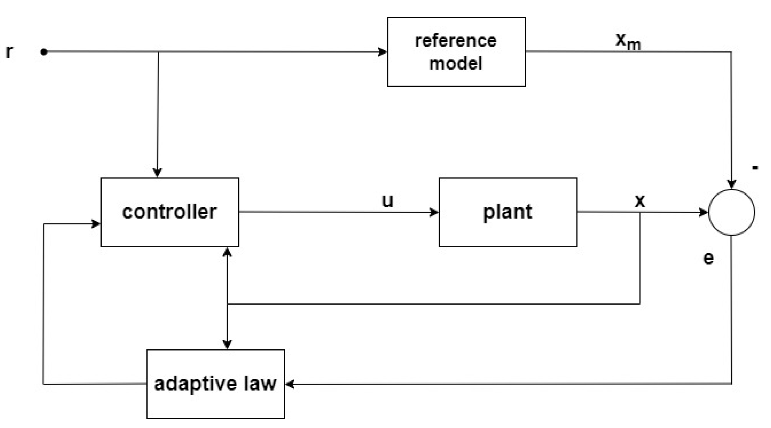
Remark 2.3: Despite the fact that equations (16), (23) and (24) ensure that the error between both the dynamical system in (15) and the reference model in (12) reduces asymptotically as , practically, the trajectory of the dynamical system can deviate significantly from the trajectory of the reference model during the learning stage (transient phase). This issue is known as the poor transient response problem.
Remark 2.4: The tracking error is an essential part of MRAC. Because the update laws (23) and (24) are influenced by this error, the control law (16) may exhibit oscillations of its own if the error includes any elevated fluctuations.
Remark 2.5: As the dynamic system’s complexity develops, it becomes more susceptible to parametric uncertainty. As a result, the typical MRAC system is incapable of providing a convenient performance. Specifically, MRAC cannot ensure that the error will converge to zero practically.
2.3.2. Modified MRAC
Motivating from the prior remarks on MRAC performance, our goal is to ensure that the tracking errors vanish asymptotically and to improve MRAC transient response. This will be accomplished by modifying the MRAC control law (16) to include the nullspace parameterization provided by the Greville formula in equation (9).
The following is a proposal for a null control vector () that is projected through a projection matrix () to act on the control coefficient’s nullspace and it is chosen to be a function of tracking error to speed up the error dynamics.
Where is the gain of the null control vector and it will be adaptively generated using the Lyapunov candidate function.
Now, the control law for the modified MRAC can be written in the following form
This implies the following:
Remark. 2.6:
Despite the fact that the expression for given by (11) contains the MPGI function , still maintains bounded due to the fact that it is a projection matrix function.
Equation (28) must be enforce the tracking errors to dissipate asymptotically in such a way that
This implies that the error dynamics can be expressed as
By utilizing the matching conditions in Assumption 1. and substituting (30) and (12) in equation (32), the error dynamics of the modified MRAC is obtained as follows
Remark 2.7: According to the description of the error dynamics (33), the projected null control vector on the nullspace of control coefficients is composed of a gain that is adaptively adjusted in response to the tracking error, which plainly effects the system error. The update law is prevented from learning from the oscillations content of the system error in this manner.
The following is Lyapunov candidate function that we will use to derive the adaptive parameters.
Now, the derivative of Lyapunov function is obtained as:
By using the properties of trace, equation (35) can be formulated as
Then,
Now the adaptive parameters can be constructed as
Theorem 1.
Considering the dynamical system obtained by equation (15), the reference model denoted by equation (12), and the control law obtained by equation (28), with accordance to equations (42), (43), and (44). Hence, the trajectory provided by equation (33) ensured that the tracking errors vanish asymptotically.
Proof of Theorem 1.
Equation (45) will result in are really bounded and hence
Now by checking the derivative of , we can prove that it is uniformly continuous.
Because are bounded by the fact that , the trajectories is bounded due to and are bounded, reference signal is also bounded, hence, is obviously uniformly continuous. This explain that , and as , and hence the error dynamics achieve asymptotic stability. □
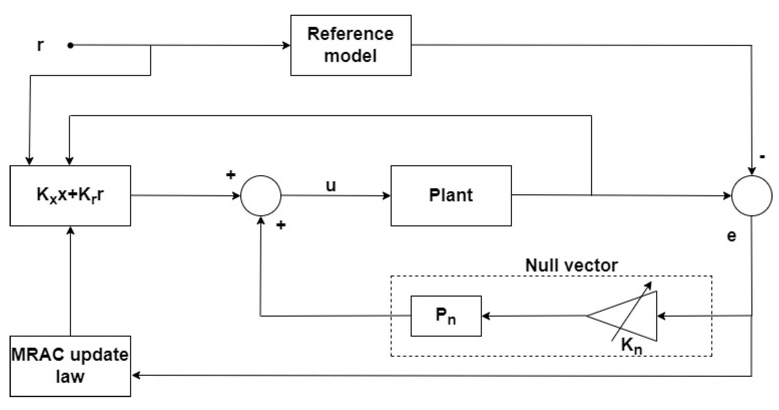
Remark 2.8: Theorem 1 emphasizes stability and good performance during both the transient and steady-state periods. Clearly , implying that the state trajectories asymptotically approaches the reference model of equation (12). Additionally, the control law (28) generated based on the null control vector (27) projected by a projection matrix (11) to act on the null space of control coefficients, or in other words, it forces the dynamical system (15) to behave similarly to the reference model throughout the system’s response.
Figure 3.
Modified Model Reference Adaptive Control.
3. Application to Aircraft Longitudinal and Lateral-Directional Control
Considering flying wing aircraft as an example, this section describes how the proposed method can be implemented.
3.1. Aircraft Dynamic Model
Figure 4 depicts an illustration of flying wing aircraft. It features two sets of elevons and split drag rudders. The inboard elevons are mostly used to regulate pitch; and positive deflection is considered as symmetric downward deflection; The outboard elevons are employed to control the roll of the vehicle through differential deflection. Yaw control is handled by split drag rudders.
Equations (49) and (50) as [36] depict the dynamic model in which the sideslip angle affects both the longitudinal and lateral dynamics, resulting in longitudinal and lateral-directional coupling. The instance aircraft’s dynamic modes are listed in Table 1.
Corresponding to the structure in Figure 4, the angle of attack, sideslip angle, roll rate, pitch rate, and yaw rate have been chosen as accessible state variables for flying wing aircraft. The control variables are chosen to be , , and signifying inboard elevons (for roll), outboard elevons (for pitch), and drag rudders (for yaw).
3.2. Reference Model
As shown in Table 1, both short period and dutch roll are dynamically unstable, but the properties of roll mode are rather excellent. This means that the design of a reference model must concentrate on enhancing the aircraft’s short-period and dutch-roll modes in order to attain stability and high performance. Therefore, the yaw-pitch axis will be subjected to the dynamic constraints.
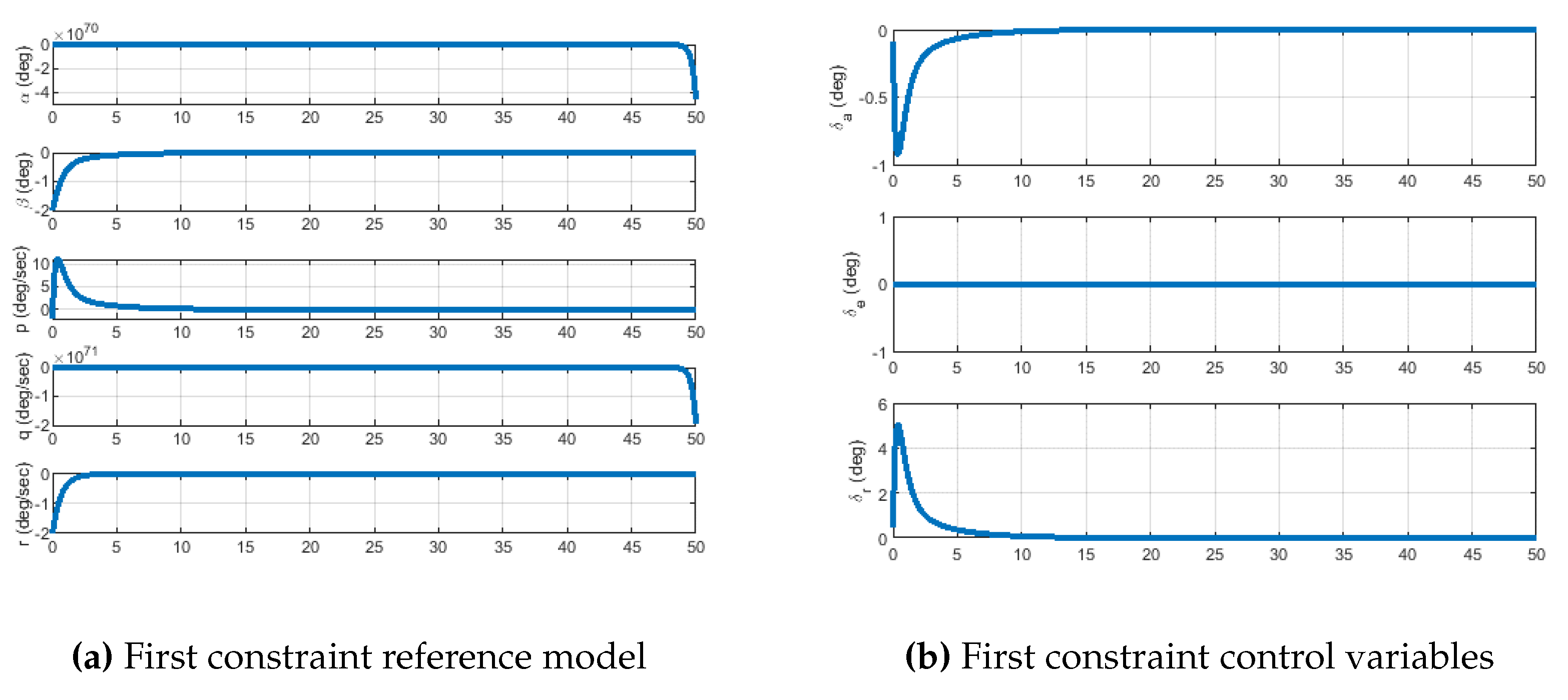
3.2.1. First Constraint {r} Configuration
Put implies that and . Hence the values of , , and are obtained by equations (6), (10), and (11) as follows
The controller that enforce the constraint is obtained as
This implies that
Table 2 demonstrates the dynamical modes of the first constraint configuration. the table shows that the first constraint configuration stabilizes the dutch-roll mode, but short-period mode is still dynamically unstable.
3.2.2. Second Constarint {q} Configuration
The state and control matrices produced from the first constraint configuration are as follows
Now, put implies that and . Hence the values of , , and are obtained as
The controller that enforce the second constraint is obtained as
Table 3 highlighted that the second constraint stabilized the modes of the aircraft i.e. is Lyapunov stable.
Figure 5.
Yaw rate constraint configuration.
3.3. Adaptive System Simulation
Simulated results are now provided to show the suggested method’s superior performance over the traditional MRAC. The resulting findings were achieved using the MATLAB software, and the computer simulation used the Ode45 as a numerical solver. The reference model adopted is Figure 6, which constrains the yaw and pitch rates.
3.3.1. First Case Study
By examining Figure 7, it is obvious that the modified MRAC method achieves precise tracking of the reference model and produces smooth trajectories. As illustrated in Figure 7b, MRAC is unable to achieve acceptable tracking performance for sideslip angle due to a minor drift in the corresponding adaptive parameter. Additionally, as a result of the learning rate, Figure 7e demonstrates oscillatory behavior. The suggested scheme overcomes these disadvantages by incorporating equation (26) into the control law of classic MRAC in order to address the tracking error problem. Furthermore, the projection matrix used in equation (11) permits the null control vector to act on the null space of control coefficients, suppressing the oscillations.
The error dynamics of both MRAC and modified MRAC are depicted in Figure 8. As illustrated in Figure 8a, the error dynamic does not totally converge to zero; additionally, it contains oscillations, which drive the adaptive parameters as seen in Figure 9. On the other hand, as illustrated in Figure 8b, the proposed method ensures that the error is convergent and free of fluctuations, corroborating theorem 2.1. The temporal history of adaptive parameters governed by modified MRAC error dynamics is depicted in Figure 10.
The control history of both methods is depicted in Figure 11. Our approach’s control response is obviously superior to that of traditional MRAC. Additionally, as illustrated in Figure 11b, the suggested scheme’s control is very similar to the control that forces the reference model to respect constraints (see Figure 6b), and hence equation (28) influences the adaptive system to behave similarly to the reference model.
3.3.2. Second Case Study
Figure 12,Figure 13,Figure 14,Figure 15 and Figure 16 have been generated with tuning gains of , , and .
Here, we would like to emphasize that the structure of the proposed scheme clearly limits adaptive parameter oscillations (as illustrated in Figure 15) and results in a reduction control input oscillations (as illustrated in Figure 16b), and thus the error dynamics of the modified MRAC (as illustrated in Figure 13b) do not encapsulate any of these oscillations.
Since adaptive parameters and control inputs have minimized oscillations, the trajectory of the states for the modified MRAC scheme will have to be smooth, as illustrated in Figure 12.
4. Conclusions
This article contributes to existing research in model reference adaptive control theory, by presenting a generalized dynamic inversion and null space parameterization. The adaptive system’s closed-loop simulations reveal a highly satisfying performance concerning guaranteed error convergence asymptotically to zero and better transient response. The developed GDI control law is separated into two sections: the first section is referred to as the particular section, and it was used to formulate the reference model trajectories by applying the stipulated dynamic constraints on the system. The other component is the null control vector, which was projected onto the null space of control coefficients and then supplemented into the MRAC control law to enhance performance. The effective implementation of GDI demonstrates that this approach has the potential to simplify adaptive control problems by eliminating the need for complex and tedious procedures. The article’s future work will include robustizing the approach versus nonlinear uncertainty and measurement noise, as well as developing a null control vector to account for these non-parametric uncertainties.
Author Contributions
Conceptualization and methodology, A.M.F; software and result discussions, A.M.F;resources, A.M.F; writing and original draft preparation, A.M.F.; review and editing, A.H.B; supervision and administration, A.H.B. All authors have read and agreed to the published version of the manuscript.
Funding
This research received no external funding.
Conflicts of Interest
The authors declare no conflict of interest.
References
- Narendra, K.S.; Annaswamy, A.M. Stable adaptive systems; Courier Corporation, 2012.
- Åström, K.J.; Wittenmark, B. Adaptive control; Courier Corporation, 2013.
- Sastry, S.; Bodson, M. Adaptive control: stability, convergence and robustness. Courier Corporation 2011. [Google Scholar] [CrossRef]
- Duarte, M.A.; Narendra, K.S. Combined direct and indirect approach to adaptive control. IEEE Transactions on Automatic Control 1989, 34, 1071–1075. [Google Scholar] [CrossRef]
- Slotine, J.J.E.; Li, W. Composite adaptive control of robot manipulators. Automatica 1989, 25, 509–519. [Google Scholar] [CrossRef]
- Nakanishi, J.; Farrell, J.A.; Schaal, S. Composite adaptive control with locally weighted statistical learning. Neural Networks 2005, 18, 71–90. [Google Scholar] [CrossRef] [PubMed]
- Lavretsky, E. Combined/composite model reference adaptive control. IEEE Transactions on Automatic Control 2009, 54, 2692–2697. [Google Scholar] [CrossRef]
- Patre, P.M.; MacKunis, W.; Johnson, M.; Dixon, W.E. Composite adaptive control for Euler–Lagrange systems with additive disturbances. Automatica 2010, 46, 140–147. [Google Scholar] [CrossRef]
- Boyd, S.; Sastry, S.S. Necessary and sufficient conditions for parameter convergence in adaptive control. Automatica 1986, 22, 629–639. [Google Scholar] [CrossRef]
- Loria, A. Explicit convergence rates for MRAC-type systems. Automatica 2004, 40, 1465–1468. [Google Scholar] [CrossRef]
- Krstić, M.; Kokotović, P.V.; Kanellakopoulos, I. Transient-performance improvement with a new class of adaptive controllers. Systems & Control Letters 1993, 21, 451–461. [Google Scholar]
- Datta, A.; Ioannou, P.A. Performance analysis and improvement in model reference adaptive control. IEEE Transactions on Automatic Control 1994, 39, 2370–2387. [Google Scholar] [CrossRef]
- Sun, J. A modified model reference adaptive control scheme for improved transient performance. IEEE Transactions on Automatic Control 1993, 38, 1255–1259. [Google Scholar] [CrossRef]
- Miller, D.E.; Davison, E.J. An adaptive controller which provides an arbitrarily good transient and steady-state response. IEEE Transactions on Automatic Control 1991, 36, 68–81. [Google Scholar] [CrossRef]
- Huang, J.T. Sufficient conditions for parameter convergence in linearizable systems. IEEE Transactions on Automatic Control 2003, 48, 878–880. [Google Scholar] [CrossRef]
- Cao, C.; Hovakimyan, N. Design and analysis of a novel adaptive control architecture with guaranteed transient performance. IEEE Transactions on Automatic Control 2008, 53, 586–591. [Google Scholar] [CrossRef]
- Landau, I. A survey of model reference adaptive techniques—Theory and applications. Automatica 1974, 10, 353–379. [Google Scholar] [CrossRef]
- Duarte, M.A.; Narendra, K.S. Combined direct and indirect approach to adaptive control. IEEE Transactions on Automatic Control 1989, 34, 1071–1075. [Google Scholar] [CrossRef]
- Slotine, J.J.E.; Li, W. Composite adaptive control of robot manipulators. Automatica 1989, 25, 509–519. [Google Scholar] [CrossRef]
- Lavretsky, E. Combined/composite model reference adaptive control. IEEE Transactions on Automatic Control 2009, 54, 2692–2697. [Google Scholar] [CrossRef]
- Bechlioulis, C.P.; Rovithakis, G.A. Adaptive control with guaranteed transient and steady state tracking error bounds for strict feedback systems. Automatica 2009, 45, 532–538. [Google Scholar] [CrossRef]
- Na, J.; Chen, Q.; Ren, X.; Guo, Y. Adaptive prescribed performance motion control of servo mechanisms with friction compensation. IEEE Transactions on Industrial Electronics 2013, 61, 486–494. [Google Scholar] [CrossRef]
- Eugene, L.; Kevin, W.; Howe, D. Robust and adaptive control with aerospace applications, 2013.
- Annaswamy, A.; Lavretsky, E.; Dydek, Z.; Gibson, T.; Matsutani, M. Recent results in robust adaptive flight control systems. International Journal of Adaptive Control and Signal Processing 2013, 27, 4–21. [Google Scholar] [CrossRef]
- Morse, A.S. High-order parameter tuners for the adaptive control of linear and nonlinear systems. In Systems, models and feedback: Theory and Applications; Springer, 1992; pp. 339–364.
- Miller, D.E.; Davison, E.J. An adaptive controller which provides an arbitrarily good transient and steady-state response. IEEE Transactions on Automatic Control 1991, 36, 68–81. [Google Scholar] [CrossRef]
- Bajodah, A. Generalised dynamic inversion spacecraft control design methodologies. IET control theory & applications 2009, 3, 239–251. [Google Scholar] [CrossRef]
- Bajodah, A. Asymptotic generalised dynamic inversion attitude control. IET Control Theory & Applications 2010, 4, 827–840. [Google Scholar]
- H. Bajodah, A. Asymptotic perturbed feedback linearisation of underactuated Euler’s dynamics. International Journal of Control 2009, 82, 1856–1869.
- Bajodah, A.H. Servo-constraint generalized inverse dynamics for robot manipulator control design. 2009 IEEE International Conference on Control and Automation. IEEE, 2009, pp. 1019–1026.
- Greville, T. The pseudoinverse of a rectangular or singular matrix and its application to the solution of systems of linear equations. SIAM review 1959, 1, 38–43. [Google Scholar] [CrossRef]
- Ben-Israel, A.; Greville, T.N. Generalized inverses: theory and applications; Vol. 15, Springer Science & Business Media, 2003. [CrossRef]
- Bajodah, A.H.; Hodges, D.H.; Chen, Y.H. Inverse dynamics of servo-constraints based on the generalized inverse. Nonlinear Dynamics 2005, 39, 179–196. [Google Scholar] [CrossRef]
- Narendra, K.S.; Annaswamy, A.M. Stable adaptive systems; Courier Corporation, 2012.
- Tao, G. Adaptive control design and analysis; Vol. 37, John Wiley & Sons, 2003.
- Lixin, W.; Zhang, N.; Ting, Y.; Hailiang, L.; Jianghui, Z.; Xiaopeng, J. Three-axis coupled flight control law design for flying wing aircraft using eigenstructure assignment method. Chinese Journal of Aeronautics 2020, 33, 2510–2526. [Google Scholar]
Figure 1.
Block diagram of Generalized Dynamic Inversion control.
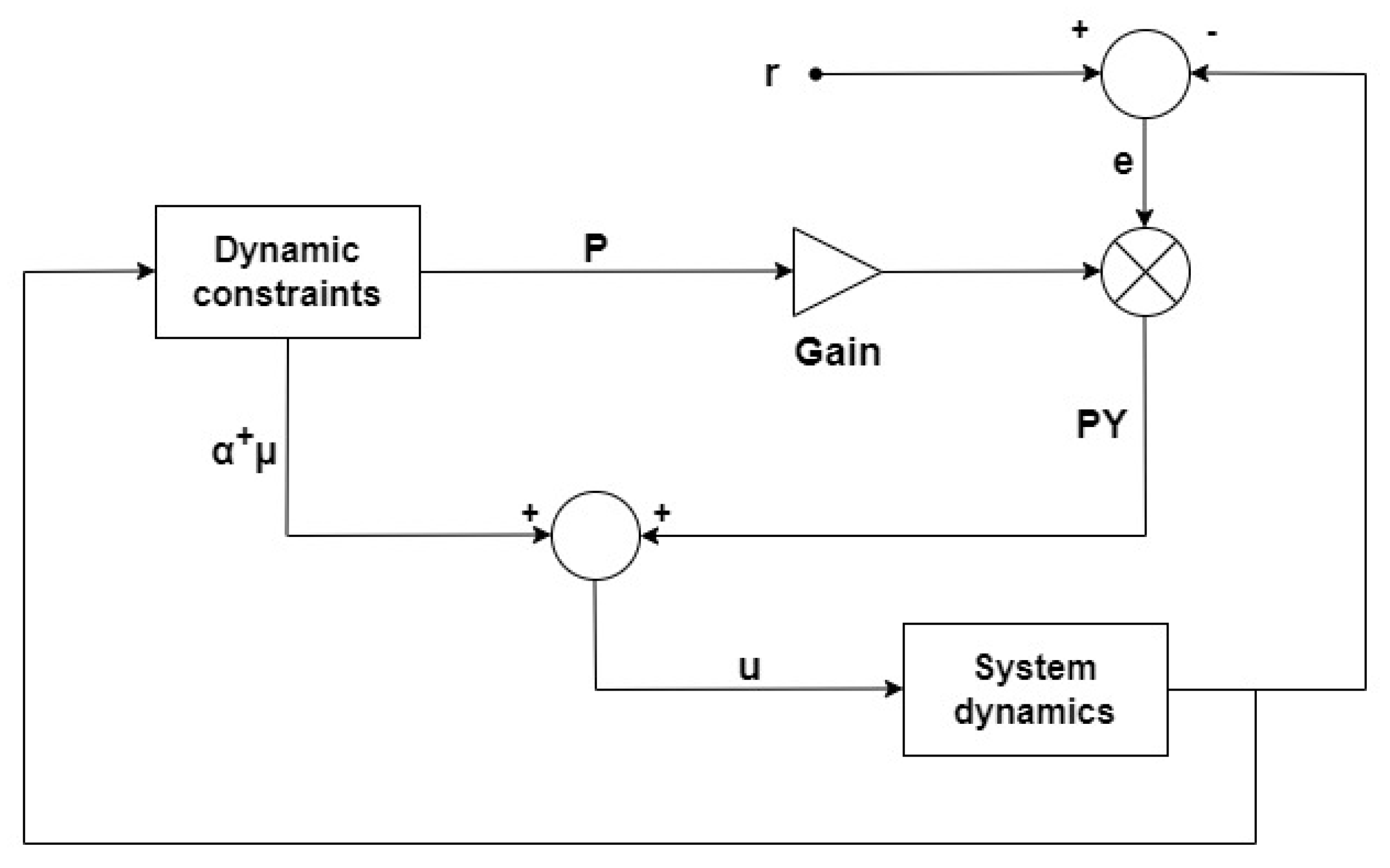
Figure 4.
Flying Wing Aircraft.
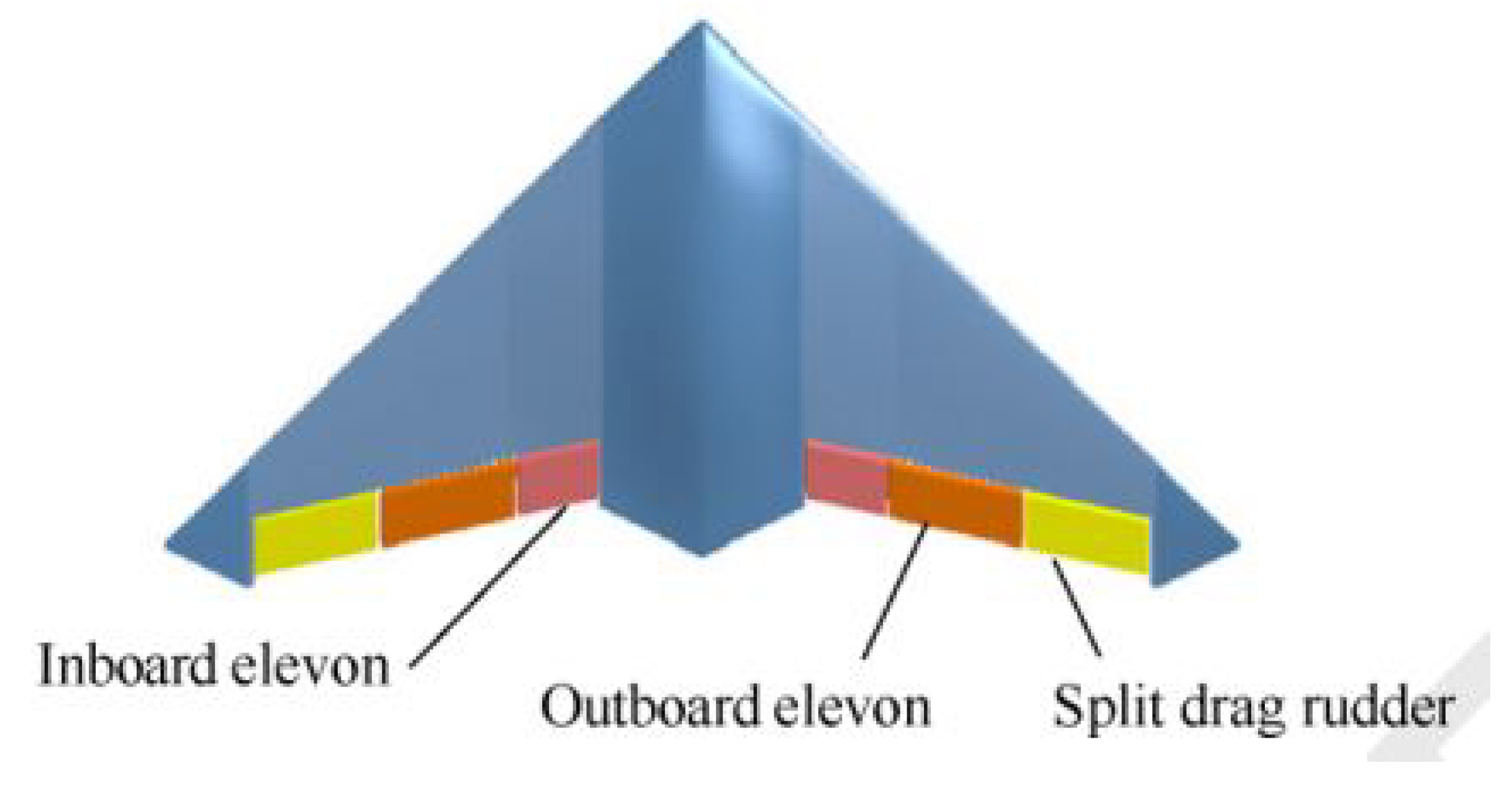
Figure 6.
Yaw and pitch rates constraint configuration vs. t.
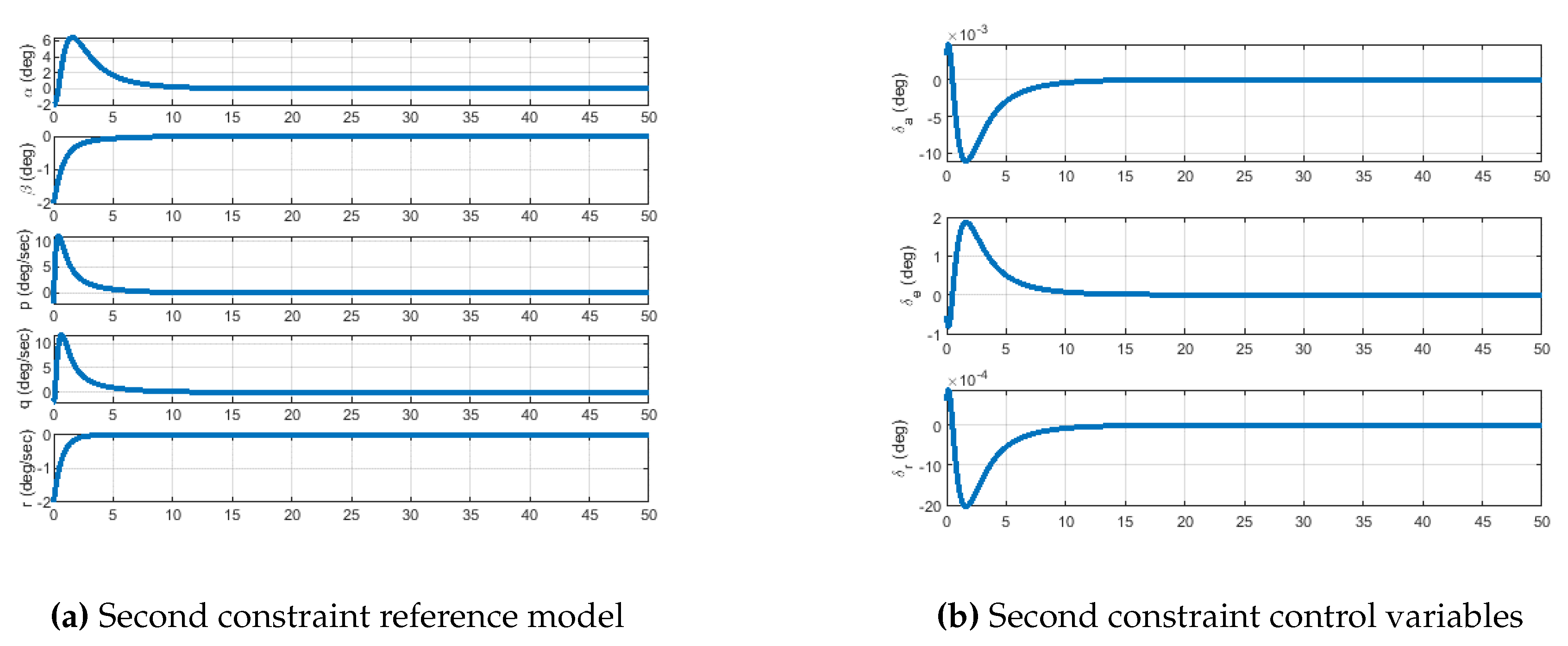
Figure 7.
System states with Reference, MRAC, and Modified MRAC.
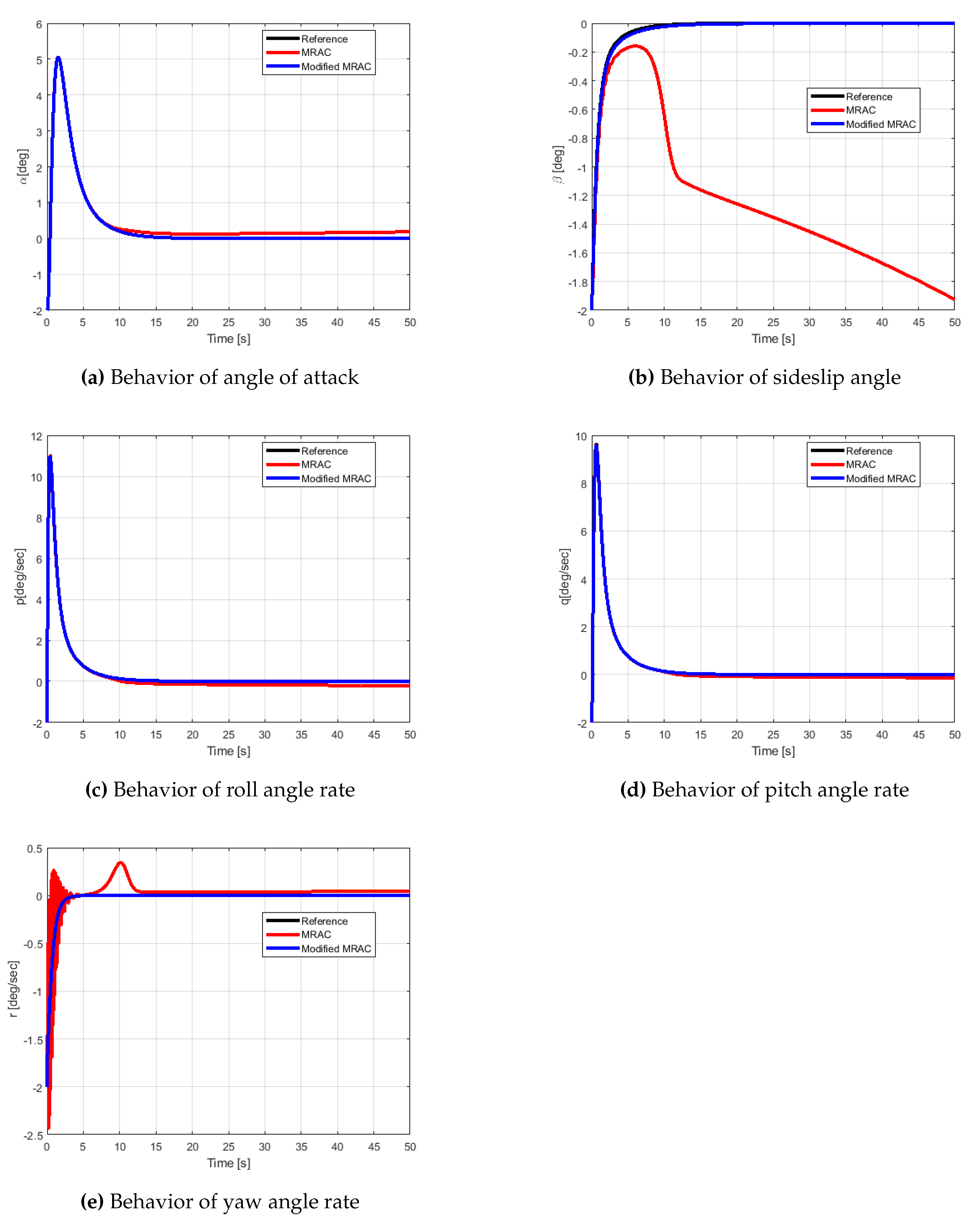
Figure 8.
Error dynamics with MRAC and modified MRAC.
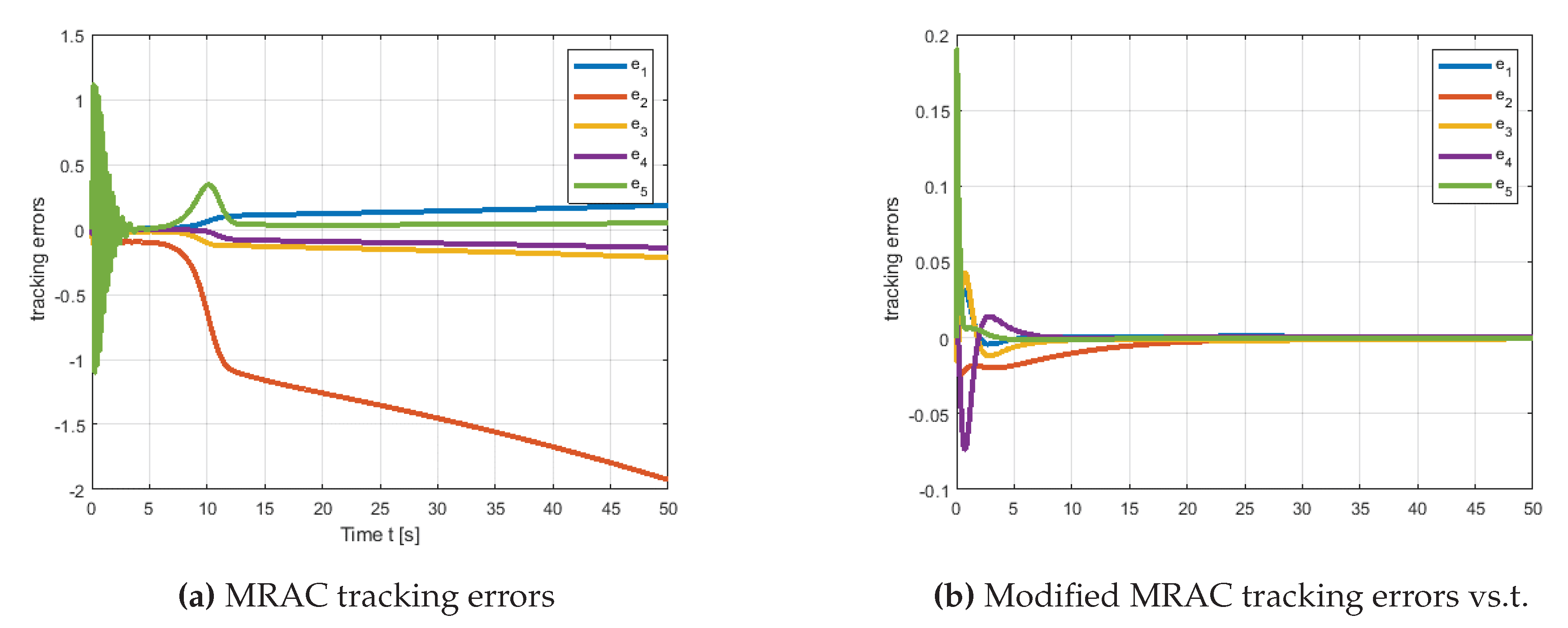
Figure 9.
MRAC adaptive parameters.
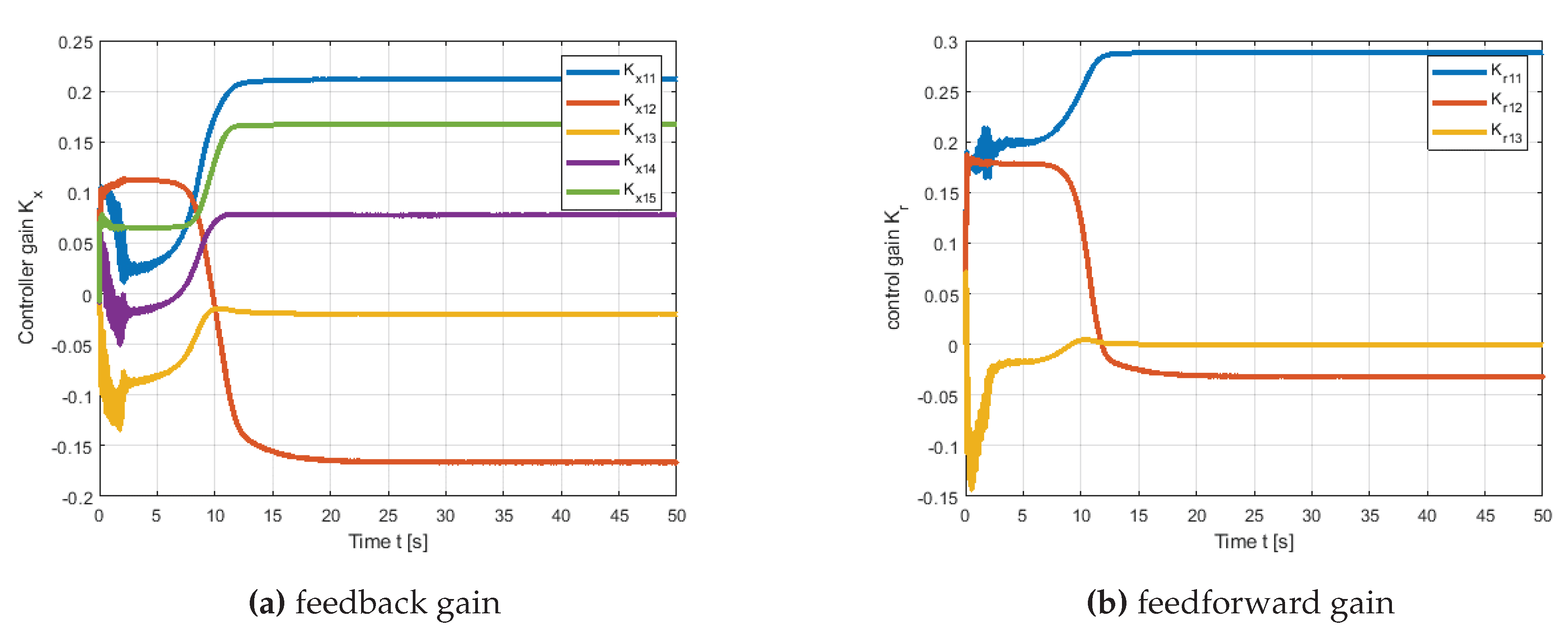
Figure 10.
Modified MRAC adaptive parameters.
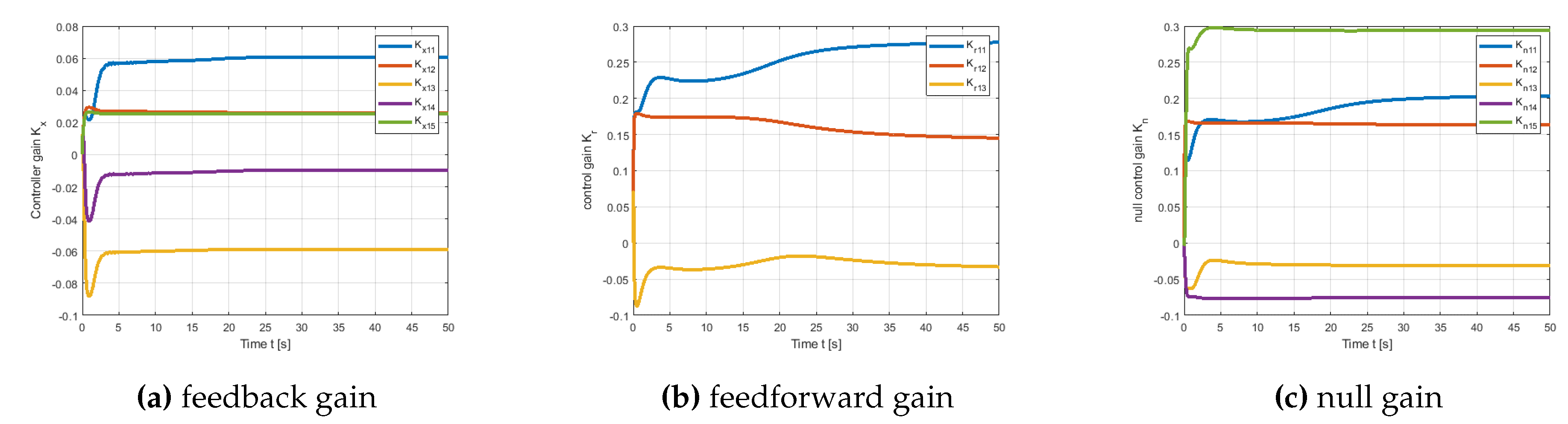
Figure 11.
MRAC and modified MRAC control commands.
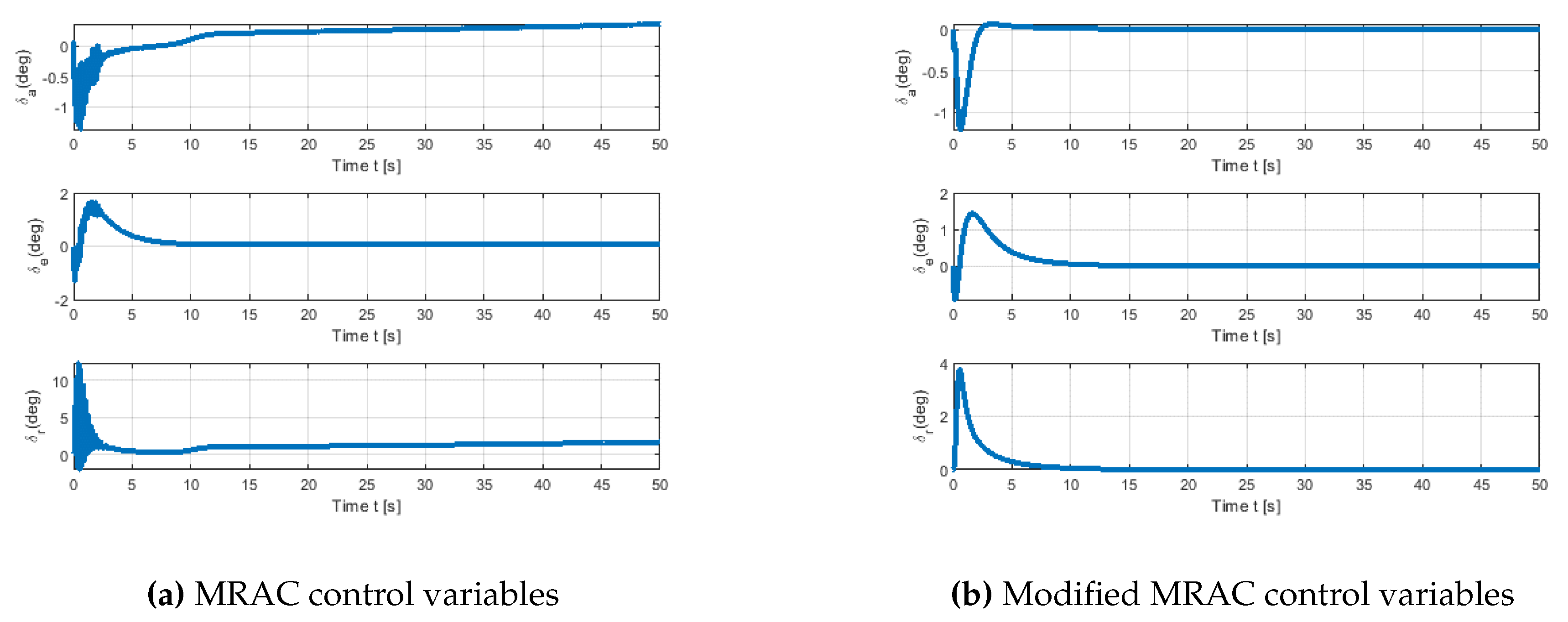
Figure 12.
System states with Reference, MRAC, and Modified MRAC.
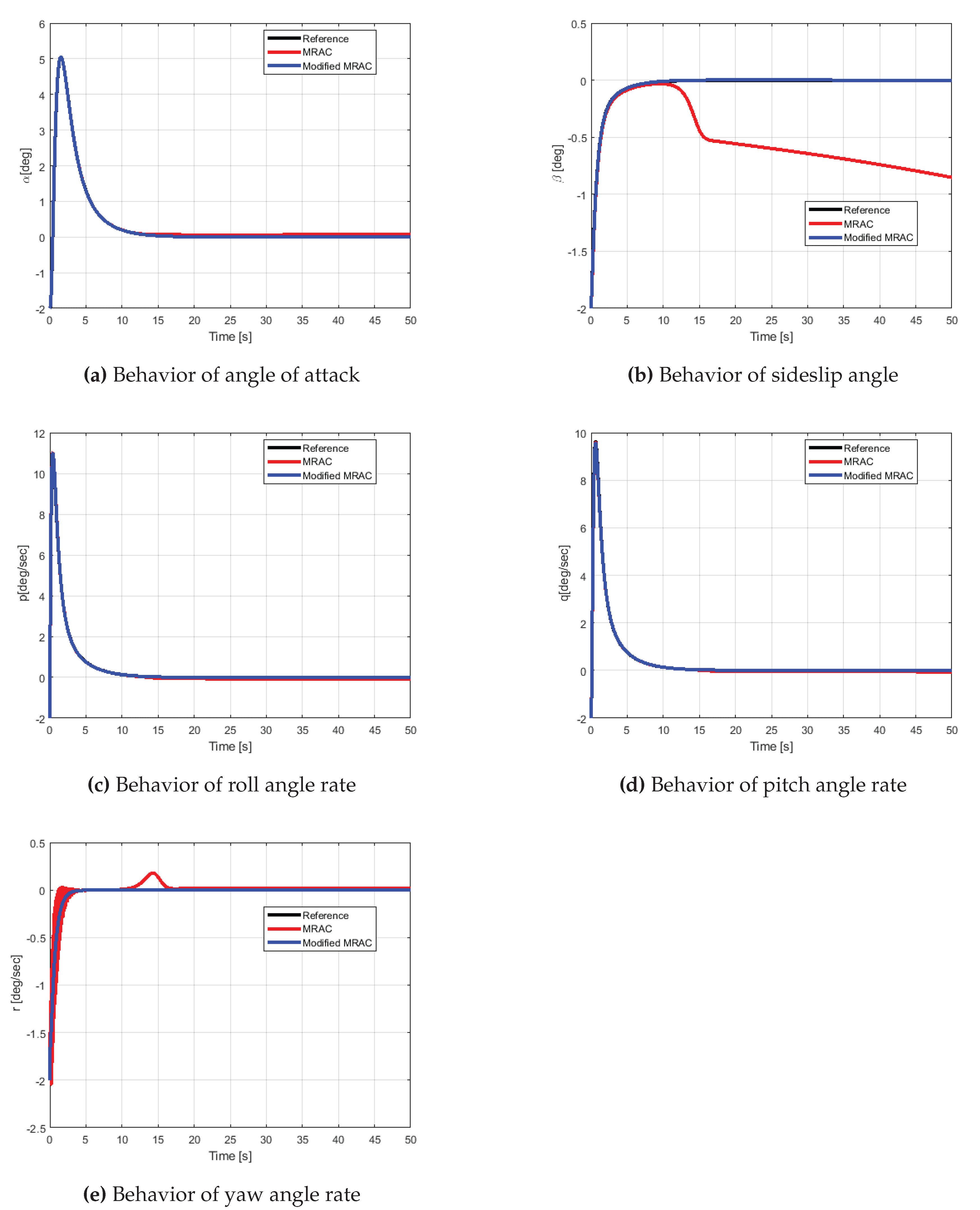
Figure 13.
Error dynamics with MRAC and modified MRAC.
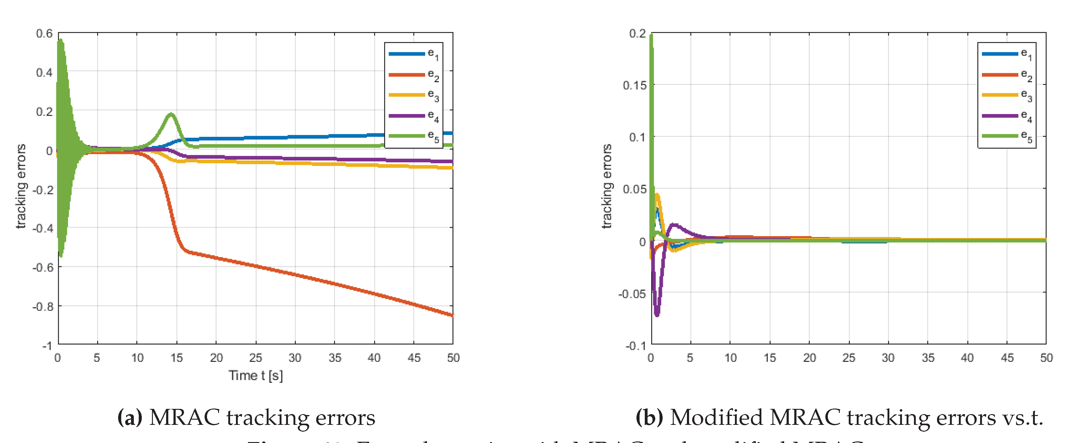
Figure 14.
MRAC adaptive parameters.
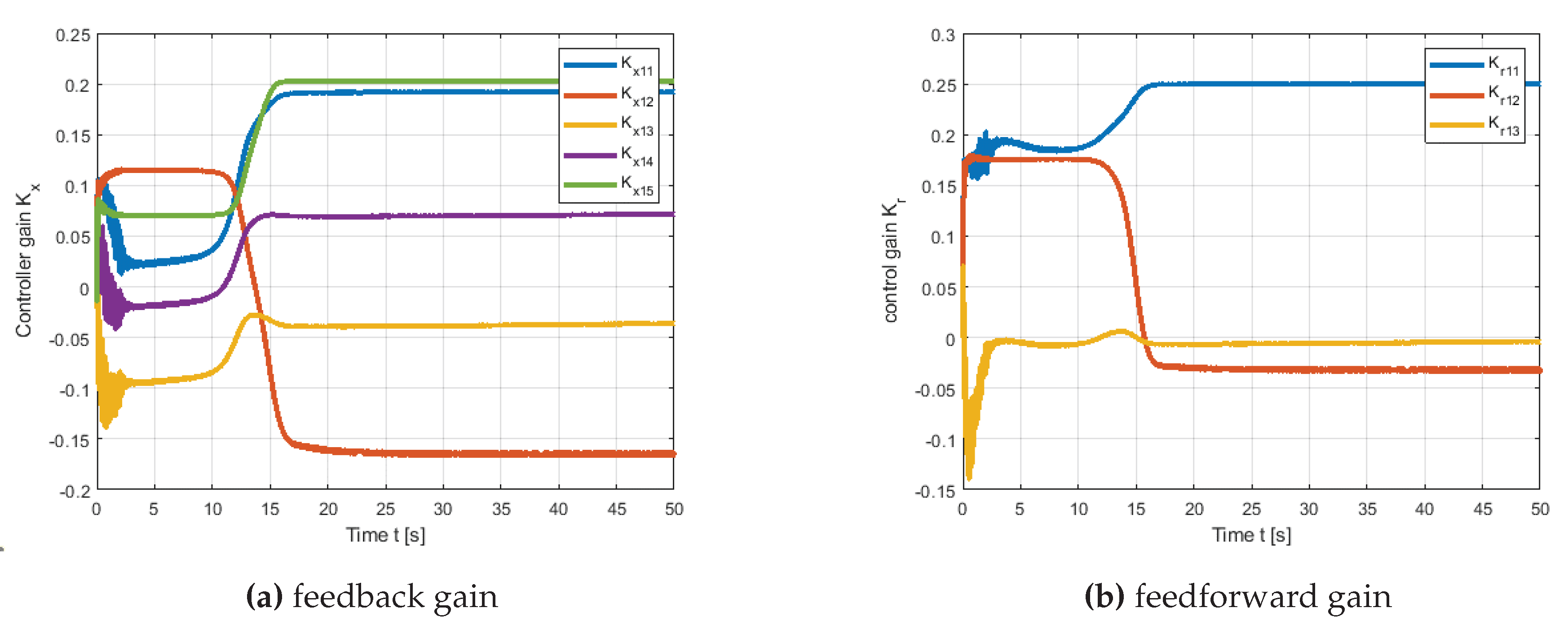
Figure 15.
Modified MRAC adaptive parameters.
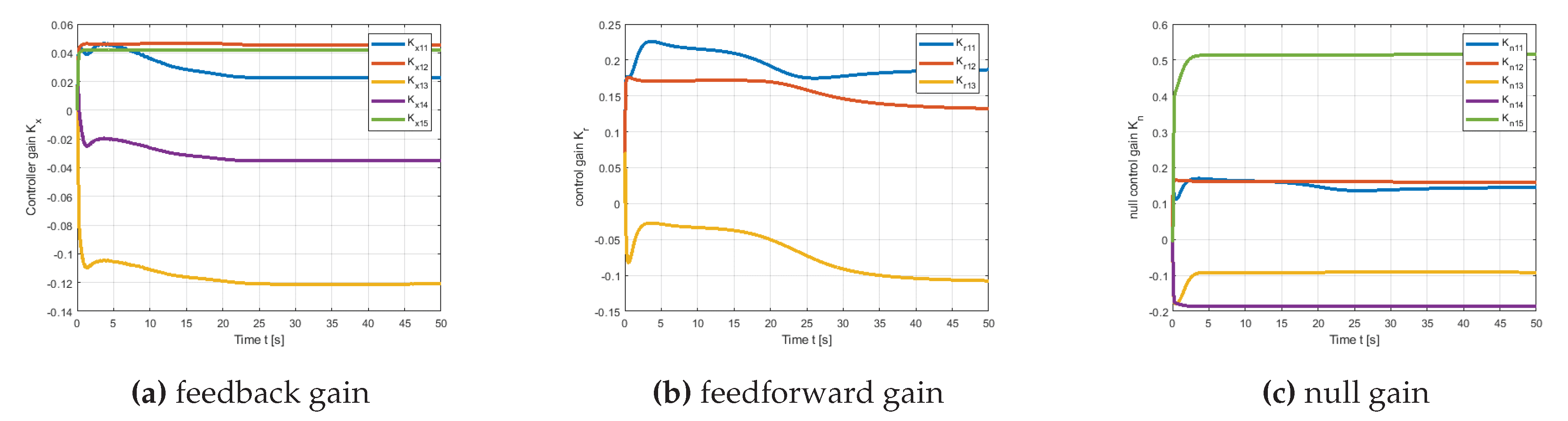
Figure 16.
MRAC and modified MRAC control commands.
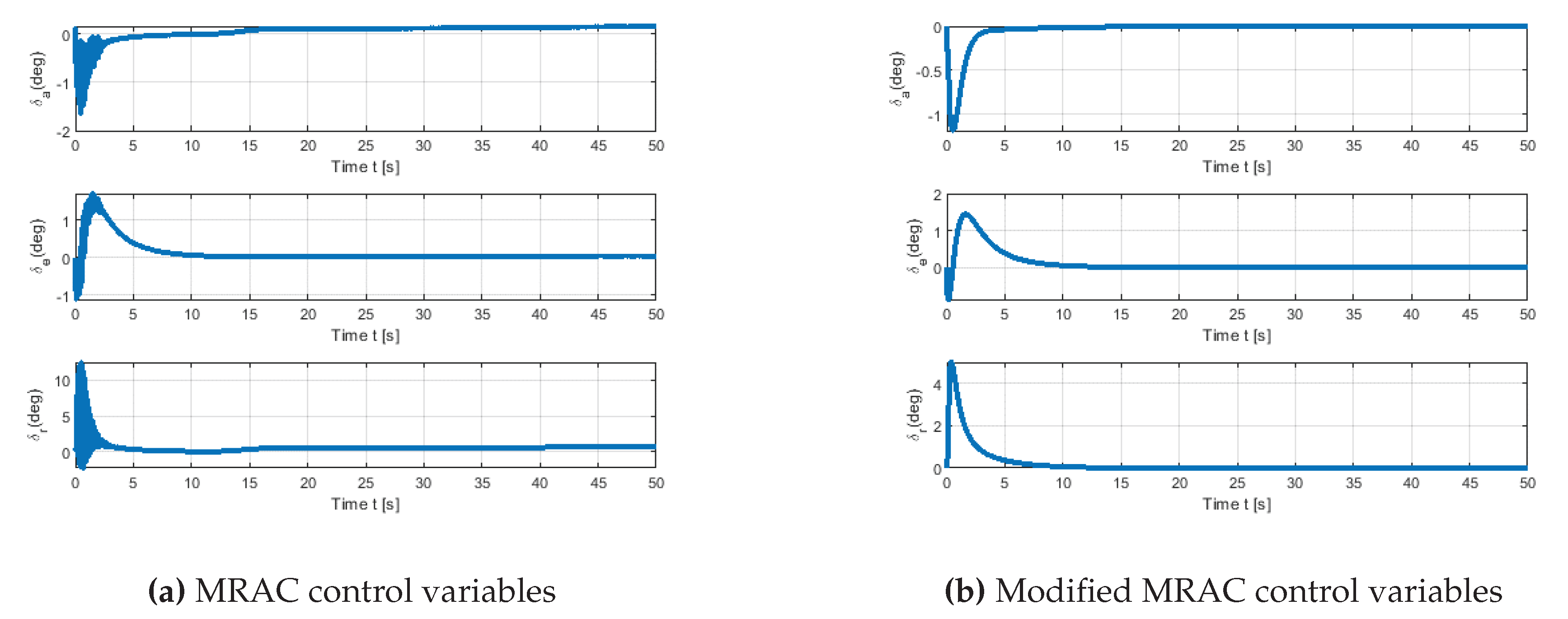

Table 1.
Aircraft Dynamic Modes.
| Mode | Eigen value |
|---|---|
| Short period | -9.4949 |
| 3.2511 | |
| Dutch roll | -3.6965 |
| 2.4777 | |
| Roll subsidence | -12.0279 |
Table 2.
First constraint Dynamic Modes.
| Mode | Eigen value |
|---|---|
| Short period | 3.2511 |
| -9.4949 | |
| Dutch roll | -0.3139 |
| -1.5 | |
| Roll subsidence | -4.6623 |
Table 3.
Second constraint Dynamic Modes.
| Mode | Eigen value |
|---|---|
| Short period | -5.0931+0.53939i |
| -5.0931-0.53939i | |
| Dutch roll | -0.3485 |
| -1.5 | |
| Roll subsidence | -0.8783 |
Disclaimer/Publisher’s Note: The statements, opinions and data contained in all publications are solely those of the individual author(s) and contributor(s) and not of MDPI and/or the editor(s). MDPI and/or the editor(s) disclaim responsibility for any injury to people or property resulting from any ideas, methods, instructions or products referred to in the content. |
© 2024 by the authors. Licensee MDPI, Basel, Switzerland. This article is an open access article distributed under the terms and conditions of the Creative Commons Attribution (CC BY) license (http://creativecommons.org/licenses/by/4.0/).
Copyright: This open access article is published under a Creative Commons CC BY 4.0 license, which permit the free download, distribution, and reuse, provided that the author and preprint are cited in any reuse.


