
Submitted:
16 July 2024
Posted:
17 July 2024
You are already at the latest version
Abstract
Hyperspectral imaging data holds great potential for various stages of the mining life cycle in active and abandoned mines. The technology, however, has yet to achieve large-scale industrial implementation and acceptance. While hyperspectral satellite im-agery yields high spectral resolution, high signal-to-noise ratio (SNR), and global availability with breakthrough satellite sys-tems like EnMAP, EMIT, and PRISMA, limited spatial resolution poses challenges for mining sectors, which require decimeter- to centimeter-scale spatial resolution for applications such as reconciliation, ore/waste estimates, geotechnical assessments, and en-vironmental monitoring. Hyperspectral imaging from drones (Uncrewed Aerial Systems; UASs) offers high spatial resolution data relevant to the pit/ mine scale, with the capability for frequent, user-defined re-visit times. Collecting data in the visible to near and shortwave infrared (VNIR-SWIR) wavelength regions offers to detect different minerals and surface alteration patterns, potentially revealing crucial information for exploration, extraction, re-mining, waste remediation, and rehabilitation. In this paper, we review of applicable instrumentation, software components, and relevant studies deploying hyperspectral imaging in or appropriate to the mining sector, especially for hyperspectral VNIR-SWIR UASs. If directly applicable, draw on previous insights derived from airborne, satellite, and ground-based imaging systems. We also discuss common practices for UAS survey planning and sampling considerations for interpretation.

Keywords:
hyperspectral imaging
; UAS
; mining
; visible near-infrared
; shortwave infrared
; mineral mapping
; waste remediation
; environmental monitoring
; drone
1. Introduction
The use of remote sensing (RS), especially imaging spectroscopy, offers large-scale, non-destructive, and time-efficient means for mineral, lithology, soil, and plant species mapping over spatially extensive areas at the deposit, camp, and outcrop scales. Imaging spectroscopy has been an active area of research for almost four decades and is based on selective absorption and reflectance of wavelengths of light by different materials. Reviews on the fundamentals are covered by e.g., Clark [1]. Van der Meer et al. [2]. Hunt [3,4,5], Hecker et al. [6], and Manolakis et al. [7]. Geological remote sensing took off with the deployment of the Airborne Visible/ infrared Imaging Spectrometer (AVIRIS) and other airborne and spaceborne instruments such as HyMap, Hyperion, Landsat series, ALI and ASTER [8,9,10,11,12,13,14,15] and has been picked up, especially by exploration both for green- and brownfield purposes using medium (5m) to low (30m) spatial resolution satellite and airborne sensors. These instruments collected either multispectral imaging (MSI) data (up to 10 different wavelength bands offering low spectral resolution) or hyperspectral imaging (HSI) data (collecting information in hundreds of narrow consecutive bands to resolve small spectral features). Satellite remote sensing, using ultra-high resolution true-color RGB imagery with a spatial resolution in the cm - dm range offers some utility for the mining industry, that low spatial resolution data (>20 m) cannot match. This includes monitoring small-scale surface changes in tailings, detecting surface expressions of subsidence, and mapping mining footprints and activities [16,17,18,19,20]. Nonetheless, since these systems are limited to visible wavelengths, they cannot be used to distinguish surface mineralogy. An uncrewed aerial system (UAS), equipped with a spectral imaging instrument, can bridge this gap and provide high spectral and spatial resolution data simultaneously. The term Uncrewed Aerial Vehicle (UAV) describes mainly the aircraft itself, UAS, commonly referred to as “drone”, includes the whole system of aircraft, including the control module, navigation hardware, transmission systems, cameras, software, the ground station and the person(s) controlling the vehicle.
While new hyperspectral spaceborne missions provide higher spectral resolution than ever before, a major impediment is limitations in the spatial resolution of the data that is not exceeding 30m [21]. For instance, tailings and Acid mine drainage (AMD)-prone surfaces have been analysed mostly via airborne or drone-borne HSI data of high spatial resolution, due to the limited spatial extent of these surfaces and associated surface patterns that need to be resolved. Although the target mineralogy is relatively well known, applying the methodology to spaceborne data is still a challenge with concerns to spatial resolution and the repeatability of the method for monitoring purposes.
Some other factors contributing to the past limited utilization of HSI data within the mining industry include:
- i.
- The sparse availability of commercial turn-key solutions, outside of core scanning systems covering both the data acquisition and analysis/interpretation.
- ii.
- Difficulties in sensing the vertical faces of a mine (which is currently being filled by ground-based and drone-based systems). Though ground-based solutions (tripod-based) have provided data on vertical faces, their deployment in an open pit environment was at -best prototypical. Some truck-mounted systems have been deployed, suggesting safer practices at open pit sites.
- iii.
- The scalability of the results from regional to close-range sensing and vice versa is an ongoing topic of research and has only recently produced comparative studies addressing the effects of scale on data interpretation.
- iv.
- The inability of 3D modelling software systems (e.g., Datamine, MinePlan, Leapfrog, Vulcan) (at least until recently) to take (semi-) quantitative mineralogical data into account, deal with complex colour-coding and display legends for 4D spectral data.
- v.
- Concerns about the repeatability of data over the highly dynamic mining sites and seasonally variable AMD. The consistency of the data over time is a challenge that has yet to be addressed fully.
- vi.
- Methodological limitations for time-relevant data acquisition, visualizations, and processing. Current techniques of data acquisition and processing are still labour-intensive, costly and time-consuming (especially for airborne hyperspectral imaging (HSI) data) and heavily rely on the expertise of the interpreter.
- vii.
- A lack of service providers in the space to offer e.g., UAS-based HSI data collection and interpretation to non-expert users in the mining industry.
- viii.
- And a shortage of well-documented and publicly available case studies with quantified, validated results and clear value propositions.
Many of these points are addressed in ongoing research projects funded by governmental or industry incentives hoping to resolve currently lacking hardware and software to fully integrate HSI. For example, EU- and national-funded projects are underway deploying UASs in the context of the critical mineral strategy and the European Raw Materials Initiative. One of these projects is the M4Mining project (Multi-scale, Multi-sensor Mapping and dynamic Monitoring for sustainable extraction and safe closure in Mining environments, www.m4mining.eu) funded by the European Union. This project aims to develop solutions for HSI UAS systems and identify data analysis and map standards for the mining industry in particular to enable an end-user-ready hardware and software solution. We strongly believe, that identifying the state-of-the-art in deploying spectral imaging within mining environments is the first step for these projects to identify the remaining challenges and opportunities and find solutions to fully integrate hyperspectral imaging in the mining industry as a standard tool.
The versatility of deploying UASs has led to their increased adoption within the mining sector. This largely involves applications based on RGB imagery and photogrammetry in stockpile volume surveying, site infrastructure inspections, and some environmental monitoring. However, UASs have the potential to act as interoperable technology with a broad range of applications that include geological pit mapping [22], geotechnical analysis, geophysical survey, rock slope stability assessment, water quality monitoring, erosion and soil loss estimation, acid mine drainage (AMD) mapping, subsidence detection and safety management (e.g., tailings dams, road haulage, etc.), rehabilitation, and post-mining environmental monitoring [23,24]. In complex environments within the mining value chain, the need for Digital Terrain Models (DTM) of high precision and high spatial resolution can be fully addressed with drones equipped with light detection and ranging (LiDAR) technology [25]. This capability can be applied in landslide mapping [26,27,28,29,30,31,32,33,34], slope monitoring [35,36,37,38], subsidence modelling [39]) and surface models [32,40,41,42]). A few studies have already presented the combined use of UAS and LiDAR with a focus on forestry and agriculture [43,44,45], UASs offer excellent performance in any environment where accurate surface representation is required, especially in inaccessible areas, along steep slopes, or hazardous environments. In such environments, undertaking a field survey with a UAS can ensure the safety of the surveyors. The cost-efficient repeatability of the survey at frequent intervals is also an advantage, that permits the comparison of the 3D surface over time so that the rates and scales of change can be detected.
With advanced sensor technology, relatively lightweight hyperspectral sensors have recently emerged covering the entire visible near-infrared (VNIR; 400-1000nm) and shortwave infrared (SWIR; 1000-2500nm) regions of the electromagnetic spectrum. Capturing data across these wavelength regions via UASs enables the mapping of a variety of materials over mining sites at high spatial resolution [46,47]. This paper reviews the application of high spatial and spectral resolution spectral imaging data in the mining industry. This review is timely as numerous papers are starting to cover the use of UAS technology in the mining industry, including some limited case studies for hyperspectral UASs for RS studies [48,49,50,51,52,53,54,55,56,57,58,59,60,61]. Although several reviews concentrate on the application of hyperspectral imaging (HSI) and RS in the broader field of geology [2,4,5,48,49,50,51,52], there is a notable absence of a comprehensive review on the state-of-the-art for HSI and its application to mining both in active and post-mining environments. We focus on the application of emerging UAS-based HSI technology, but we also examine case studies conducted using airborne and spaceborne imaging systems to understand the full potential of UAS in the mining industry and recognize the niche that UASs could fill. In this paper, we overview spectral imaging principles (Section 2), present common hyperspectral UAV systems (Section 3), and discuss the design of hyperspectral UAV studies (Section 4), including sampling and validation standards. We then review existing case studies of HSI applied in mining environments, including airborne and spaceborne platforms, to highlight the potential applications for hyperspectral UAV systems (Section 5). We conclude with a discussion of possible future applications of the technology in the mining value chain (Section 6).
2. Principles of Spectral Imaging
Imaging spectroscopy is usually referred to when measurements and analysis are taken out with hyperspectral instruments. In RS, the term “hyperspectral imaging” (HSI) or “multispectral imaging” (MSI) is more commonly used when the Earth’s surface is the object of our study. Here, speaking of both methods, we will use the term “spectral imaging”. HSI is able to resolve narrow absorption features specific to different minerals and materials. While the definition of “hyperspectral” in terms of number of bands is not rigid, the IEEE Standards Association set up a standard in 2018 for devices that cover the 0.25-2.50 µm spectral region. For a system to be considered hyperspectral it needs to exceed 32 bands [62]. Anything capturing less than 32 spectral bands is considered multispectral.
Imaging spectroscopy generates data cubes where each image pixel represents four-dimensional information, with three dimensions in the spatial x-, y, and z-coordinates, and spectral information in the fourth dimension. Data cubes are created by using the principles of spectroscopy, where the properties of light are captured across a set of continuous spectral bands to produce a characteristic spectrum on a per-pixel basis. Pushbroom RS employs an array of detectors to capture spectral imaging data of the Earth’s surface as the platform moves [62,63]. Unlike whiskbroom systems that scan across the scene with a single detector, pushbroom systems capture entire lines of data simultaneously, offering high spatial and spectral resolution. This method minimizes motion blur and enables efficient data collection by continuously recording data along the platform’s path, capturing multiple spectral bands simultaneously.
2.1. Spectral Data Analysis
With the use of VNIR and SWIR wavelength ranges, rock material from all stages of the mining value chain can be investigated by studying the characteristic absorption features, inflections, and signature slopes of the individual (pixel) spectrum captured by the imaging system. In geological environments, absorption features detected in the VNIR arise from transitional elements, including iron-bearing minerals and rare-earth elements (REEs), while the SWIR region is commonly used for identifying alteration mineral assemblages related to hydrothermal systems of base and precious metal deposits [64]. The mineral groups that can be detected and mapped in the VNIR-SWIR wavelength regions include carbonates, sulfates, sulfosalts, clays, and phyllosilicates such as chlorite, talc, and muscovite. A detailed account of the causes of absorption features can be found in [3,4,5].
Common analytical techniques for imaging spectroscopic data are divided into two broad categories: data-driven and knowledge-based approaches [65]. Data-driven approaches rely only on the data itself and some additional reference data (spectra), commonly called training classes or endmember sets, that are imported to or derived from the image data. Data-driven approaches are categorized into per-pixel (hard classifier) and sub-pixel (soft classifier) approaches with single and multiple labels for each pixel, respectively. Comparison-based per-pixel approaches, such as spectral matching with the use of a reference spectral library, include similarity-based methods such as the Spectral Angle Mapper (SAM) [66,67], least square-based methods such as least squares regression (PLSR) and learning-based approaches such as artificial neural networks (ANN) or support vector machines (SVM). Mixture-based, sub-pixel categories include partial and full unmixing methods such as mixture-tuned matched filtering (MTMF) and linear spectral unmixing (LSU). Knowledge-based approaches rely on user knowledge about the spectral behaviour of a target without the use of direct reference data to extract meaningful information from a spectrum. Knowledge-based approaches aim to estimate the quality and/or quantity of either of the main components making up a spectrum including: i) a continuum, ii) absorption bands and iii) residuals or noise. These techniques include absorption and spectral feature modeling. A common feature mapping approach in this category is “minimum wavelength mapping” (MWL). This feature-based approach retrieves the depth, minimum wavelength, area, width, and asymmetry of individual features, known as spectral parameters, for material identification and mapping [6,68,69,70,71]. The output of this technique can be fed into expert systems and decision tree structures (DT) to enable per-pixel classification. Examples of expert systems include the classic USGS Tetracorder and its modern interface called “Material Identification and Classification Algorithm” (MICA) [72,73,74]. Partial absorption modelling, clustering techniques [75], as well as various band arithmetics (e.g., band ratios), also do not require the use of pre-existing reference data. Applying these techniques results in spectral similarity and score images with varying magnitudes of the matched and inferred values and requires specialized visualization and contextualization methods to interpret the resulting output maps. Overview of the spectral processing methods available for geological RS is provided in [2,4,5,48,49,50,51,52]
2.2. Auxiliary Data Acquisition
The collection of field data is complex and highly dynamic and needs to be managed carefully for hyperspectral field campaigns including drone surveys. Field data typically includes a variety of instrument data, ancillary data (‘metadata’), as well as geographic coordinates and images, which can lead to interrelated but disjointed datasets.
The terminology here follows the TERN “Effective Field Calibration and Validation Practices” [76]. Data is considered a direct quantitative measurement of the sample in question, either via an instrument or another quantitative method (e.g., instrument readings, raw imagery). Ancillary data is considered as data collected in association with the primary dataset such as geographical coordinates, comments, date and time, descriptive information and imagery and information about the instruments being used. Metadata is considered the information regarding the discovery and the use of the data, such as scale, units, geographical and temporal scales, custodians and licensing. Careful collection of this information is important to ensure that various researchers and stakeholders can reuse the data in the future.
Field calibration and sampling strategies for remotely sensed data have recently been developed for ecological applications and provide some utility for geological surveys [76]. Clearly defined strategies are important as field surveys can be logistically challenging, especially for UAS-based HSI, influencing the quality of the survey data and associated ground sampling and calibration data. Firstly, field data collection can vary depending on the site access conditions and weather conditions. As a result of these factors, sampling strategies often get modified, leading to errors. Secondly, the equipment in larger campaigns can vary, as can the observers and their experience level, resulting in inconsistencies due to observer bias and different objectives. As a result, we suggest the principle that field methods must be discussed prior to any campaign and a consistent sampling strategy (e.g., number/density of samples, sample area dimensions etc.) and protocols (e.g., calibration procedures, repeats, blanks etc.) must be applied. We suggest following best practice such as: The use of data entry tools to minimize errors. Provide sufficient data storage via an accessible database with clearly established data licenses during and after a survey. Set up a frequent review period (annual) to identify issues, provide feedback on data completeness, identify unbalanced data collection across sites and potential data bias.
3. Best-Practice for UAS-Based Spectral Imaging
In the following sections, the current state-of-the-art hyperspectral UAS hardware and survey designs are discussed, including sampling guidelines during fieldwork to assist in data interpretation and validation. This includes best practices for UAS-based VNIR and SWIR data collection to acquire meaningful, high-quality data in mining environments. While historically UAS-based VNIR full-frame sensors have been employed for geological mapping applications [60,77,78,79], the inclusion of the SWIR wavelength ranges requires pushbroom-type data acquisition and has only recently become deployable in industry applications due to the miniaturization of cameras, smaller platforms, UAS power requirements and cooling (<-100°C) of the detectors as well as high-performance gimbals.
The inclusion of the SWIR wavelength range offers valuable information for mineral detection, but it also complicates the survey design and flight planning. The SWIR wavelength range introduces dependency on accurate measurements of atmospheric conditions, as well as geometric and radiometric correction and processing of the data. Only a limited number of publications using UAS-mounted SWIR cameras are currently available (e.g., [80,81,82,83,84]), meaning this research field is only just emerging and our understanding of good methodologies remains nascent. Similarly, the best-practice guidelines for the acquisition and correction of coaligned VNIR-SWIR datasets, and accurate georeferencing and geometrical correction of such combined datasets, remain a topic of current research.
Currently known hyperspectral camera manufacturers and service providers with different capabilities to collect data relevant to AMD detection are summarized in Table 1. The list includes systems using both pushbroom and full-frame, as well as VNIR and VNIR-SWIR cameras mounted to UAS.
3.1. Hyperspectral Pushbroom UAS Selection
A hyperspectral UAS commonly consists of an airframe platform, a hyperspectral camera, an Inertial Navigation System (INS) and Inertial Measurement Unit (IMU), and a differential Global Navigation Satellite System (GNSS). The airframe provides the platform for all components, i.e., connects the drone arms with the motors and rotors, if multirotor systems are being used, the landing gear/feet, source of energy (e.g., batteries or fuel), an adapter for a gimbal or direct camera attachment, different GNSS and radio antennas for both drone and camera, positioning LEDs and the autopilot system of the drone itself. The platform carries the batteries and payload of the gimbal and the camera. The drone’s maximum allowed take-off mass (MTOM) and certification (C-class label) dictate within which class and in which context and area the UAS can be flown and is dependent on the jurisdiction, registration and license of the drone pilot/piloting company and drone operator. This differs quite substantially between UAV manufacturers and UAS configurations and changes in different countries and jurisdictions. In European countries, European Union Aviation Safety Agency (EASA) rules and regulations [85,86,87] based on recommendations from the International Civil Aviation Organization (ICAO) [88] must be followed, including local regulations in the different countries.
While more systems exist (see Table 1) the system to base best practice guidelines on in this manuscript is a BFD SE8 octocopter carrying a Mjolnir VS-620 camera from HySpex and a LiDAR from Velodyne. This is only due to the authors’ shared experience with this particular system. It is a good representation of current hyperspectral UASs carrying both a VNIR-SWIR pushbroom imaging camera system and a co-mounted Lidar scanner. The system’s total MTOM is below 25kg as per EASA to fly in category A3/ open category §4 2019/947 . The Mjolnir VS-620 consists of a VNIR V-1240 and SWIR S-620 hyperspectral camera integrated into one chassis on two optical axes in a co-aligned field of view , a data acquisition unit operating the two sensors, an internal INS, and a radio connection to a ground station for remote access to the Mjolnir (Transmission Control Protocol/Internet Protocol link (TCP/IP)). For specifications on the cameras and UAV platform, see the hardware provider’s website. A LiDAR scanner is mounted underneath the HSI camera (Figure 1) and triggered in the same software. While the LiDAR is run independently of the hyperspectralHSI scanner, it receives time tags in the form of NMEA messages (National Marine Electronics Association) and pulse-per-second signals (PPS)) from the same INS as the HSI camera. Figure 1 shows the schematic overview of the UAS. The UAS is driven by two 25Ah lithium polymer high-voltage (LiHV) batteries. The complex interactions and components of a UAS are described in detail in [54] and is outside of the scope of this document. To reconstruct the three spatial dimensions of a pushbroom solution, the three axes representing roll, pitch and heading of each mid-exposure of each frame needs to be known with high accuracy. This movement is exaggerated in a UAS due to the lightweight platform and the high spatial resolution [54]. Therefore, this motion is captured by an additional camera-specific set of differential GNSS and IMU to correct for the movement of the camera relative to the airframe [81]. A boresight calibration accounts for the angular rotation between the IMU coordinate system and the camera coordinate system, transforming the INS data to the camera coordinate system. This is achieved via a boresight flight above well-defined Ground Control Points (GCPs) or in reference to a cartographic orthophoto and digital surface model reference. Alternatively, cross-flight pattern-based boresighting is an established standard for this aim [89]. The use of gimbals is advisable, and some might say necessary, for multirotor pushbroom UAS primarily to stabilise the imaging payload. This helps maintain a consistent orientation relative to the ground and is especially true for pushbroom systems where each line is collected with at a different time while the UAS is moving laterally, horizontally and is vibrating itself. Multirotor UAS, due to their inherent instability caused by rotor movements and environmental factors like wind, require gimbals to counteract these movements and keep the imaging payload steady. Proficient gimbal hardware and software have only recently become available for multirotor solutions and is one of the reasons why pushbroom system were previously not widely used on UASs [53].
3.2. Preparation of a Hyperspectral UAS Campaign
The first step of the study design is to determine the area of interest and the available timeframe and necessary airtime. The area that can be covered is influenced by the number of available field days, including the time for transport of equipment. Transportation of all equipment must include the transport of heavy technical components, as well as all lithium batteries, to the survey area.
It is advised to plan all individual data collection and calibration flights in advance of the campaign to gain an understanding of the area and the total necessary airtime under ideal flight conditions (wind speed, sun angle, atmospheric conditions). However, based on practical experience almost all flight plans will require adjustment in the field based on on-site conditions. Flight planning must consider the sun angle, available illumination, change in surface level and assumed related battery drainage, terrain-following capability and limits, and local legislation and limitations around uncrewed aviation. The variability in the size of the flight lines after data correction and any possible resulting data gaps in the collected data also must be considered. The authors therefore advise an overlap of 25% between individual flight lines to avoid data loss during mosaicking. The survey objective will determine the required ground pixel size or spatial resolution. This in turn dictates the optimal flight altitude and the required sampling point spread function compatible with the pixel size requirements. The speed of flight is adjusted to achieve maximum SNR. A test flight prior to the first data acquisition flight can help the operator determine the optimal integration times of the VNIR and SWIR camera to avoid over- or undersaturation in light albedo pixels. This will give information on the relationship between speed, altitude and SNR and will likely lead to compromises with the survey objective in mind. The speed of different systems will depend on the system’s light sensitivity, i.e., lenses’ F-number, pixel size on RAD and spectral sampling and will differ from system to system. To give an example, for the UAS described as an example, a good pay-off between a high spatial resolution and a high coverage per flight for flights taking place in Central Europe during summer is achieved by flying at the maximum permitted height of 120m height above ground level (AGL), resulting in a corresponding pixel size of 6cm/pixel with a ground speed between 2-4 m/s. Maximum height AGL for flight planning will differ based on drone certification, pilot competency and country regulations.
The changes of sun angle and illumination strength during the day determine the optimal data acquisition timeframe. The best illumination is available around midday (sun close to solar noon), and it is recommended that surveys are planned closely around this timeframe, with solar zenith angle lower than 70° (optimal) or lower than 80° (acceptable). However, when dealing with steep terrain, areas of interest might only be illuminated at certain times of the day (especially important for vertical drone or tripod measurements). The weather is a key factor that must be considered at the planning stage, as well as in the field. The questions to be asked are: What is the weather expected to be like at the study location? How quickly does it change? What are the operating boundaries of the used drone? Rain poses a significant threat to the success of the campaign and cloud cover detrimentally affects the quality of the HSI data. Depending on the drone manufacturer and the confidence of the pilots, the wind speed and likelihood of gusts must also be considered. [54] suggest a windspeed of <5m/s as best practice for multi-rotor systems. Optimal boundary conditions for high-quality data are a solar zenith angle lower than 70°, a cloud-free sky and dry rock surfaces.
The exemplary system described in here achieves approximately 12 minutes of total flight time per flight, including ca. 9 minutes for data acquisition, two alignment flights prior and post data acquisition and take-off and landing. These 12 minutes are influenced further by air temperature, wind speed, changes in terrain surface level and the gradient of these changes, speed/ampere during battery charging, the take-off position and its distance to the area of interest, fail-safe procedures, wildlife interference, and pilot confidence. Including the preparation time before and after landing, one flight adds up to 30 minutes including the 12 minutes of airtime. Depending on the weight of the payload, i.e., if an additional LiDAR is mounted or not, flight time can increase up to 25 min. Figure 2 shows the drone platform carrying the HSI camera and LiDAR payload from the pilot perspective.
3.3. Execution of a Hyperspectral UAS Campaign
We advise using the first flight of the day as a test flight for the drone to collect data and calibrate the INS. Calibrating the internal camera magnetometer of the APX to the new current location is also advised. Always follow the UAV manufacturer’s recommendations for the instruments necessary to enable autopiloting and navigation i.e., if AGL is set correctly. If accurate Digital Surface Models (DSMs) for flight planning are not available, a LiDAR-only flight can be carried out for an accurate surface model of the study area. This could also be achieved with a smaller drone that offers a 3D DSM surface reconstruction through photogrammetry workflows. A detailed DSM of the study area allows for precise flight planning and adjustment of the preferred flight altitude (e.g., to ensure that 120m AGL are kept), a constant pixel size and precise fail-safe procedures. It also is necessary to accurately mosaic individual flight lines from each flight. Ideally, the DSM is available before the survey. In addition to the acquisition of hyperspectral data, data from different sensors is also usually collected, to improve the correction of the HSI and aid the interpretation of the collected data.
Auxiliary data collected alongside the flight campaign often includes the collection of ground-truthing data for interpretation (including spectral and/or physical samples for physiochemical testing). The collection of additional data to calibrate the drone-based data for reflectance is not necessarily imperative and depends on the study’s overall objective. Examples include collecting downwelling irradiance, using sky-ward videography to record visual changes in atmospheric conditions, and by placing large homogeneous (often calibrated) reference panels in the field of view (FOV) of the UAS survey [54].
3.4. Data Correction and Post-Processing
The geocoding of the pushbroom hyperspectral data is done by forward ray tracing from the sensor position to a readily available digital surface model. This can either be done in a raster representation or a projection onto a surface mesh. The result of such a correction is a set of x/y/z coordinates for each hyperspectral image pixel, i.e., a ‘hyperspectral point cloud’, which is a standard output of (e.g.,) the PARGE software [89]. Starting from this representation, the geometry for each pixel is well described and can be used directly for visualization, rectification to a standard grid or for terrain-based simulations. The latter is important to estimate the irradiance at the spectral image data position.
The radiometric data correction and post-processing routines detailed here are based on the industry standard “Drone atmospheric correction method” (DROACOR) [90,91,92] . The previously mentioned gathered auxiliary data can be included in the data correction and post-processing. The necessary information for processing the data in the DROACOR software are the time of day, location (LAT/LON), solar and observation angles, terrain height, platform altitude, and the sensor internal geometry. DROACOR uses a physical inversion process from at-sensor radiance to ground reflectance based on pre-calculated Look-up-Tables (LUT), based on the Libradtran radiative transfer code [93]. Thus, the HSI data must be calibrated traceably. For uncalibrated data, an inflight calibration based on calibrated reflectance targets can be performe, alternatively. Some more information is gathered directly from the acquired images prior to the reflectance retrieval. This parametrization consists of four steps for HSI: i) an estimation of the aerosol optical thickness at 550 nm, ii) an (optional) inflight radiometric calibration using the aforementioned calibrated reflectance target, iii) a spectral shift detection and correction based on atmospheric absorption features and adaption of look-up-tables (LUTs), iv) an estimation of the total column of atmospheric water vapour. The estimation of the water vapour and aerosol optical thickness are retrieved from the average image spectrum using spectral fitting to simulated at-sensor radiance spectra. The sensor-specific atmospheric LUT can be created based on the spectral recalibration as a subset of a more generic LUT [70].
The main processing step of DROACOR is the reflectance retrieval relying on the calibrated at-sensor radiance data. The reflectance retrieval uses the relative distance between the earth and the su and the observation angles to derive the path scattered radiance, the direct solar ground flux, the diffuse flux, and the off-nadir and diffuse ground-to-sensor transmittance on a per-pixel basis. The adjacency effect from nearby objects created by the atmospheric scattering is relevant for low altitude data acquisitions specifically for the irradiance term, which is governed not only by the direct illumination but also by aerosol scattering and indirect scattering affected by the neighbouring pixels. Wavelength within regions known for high atmospheric feature absorption can be removed or interpolated to keep a continuous spectrum. After the (optional) polishing of the reflectance data , the variable illumination in terrain and the bidirectional reflectance distribution function (BRDF) effects can be corrected. The goal of the topographic illumination correction is to transform the first-order bottom of atmospheric reflectance (“scaled or apparent reflectance”) to spectral albedo values (“absolute reflectance”). DROACOR handles this by a modified Minnaert approach which ensures that the effect of BRDF is not overcorrected. If a system with a large FOV is used, the BREFCOR method can be applied which corrects the BRDF effect considering the observation angle [91].
3.5. Sampling and Validation in Geological Remote Sensing Studies
The wide range of geological RS data products are mostly validated based on either on-site physical sampling for subsequent laboratory-based geochemical analysis or in situ observations and measurements. Sampling is usually approached from a geochemical perspective, though the ethical aspect of sampling is not to be discarded. While geochemical sampling for exploration or environmental studies is extensively covered in different textbooks (i.e., [94]), the focus is largely on randomization of sampling to avoid bias, considerations for sample medium (rock vs soil vs water), sampling interval, grain size fraction, sampling depth, and background variation among others. The ethics of sampling geological sites is discussed less frequently, see [95]. These practices include: the “leave no trace” approach, acquiring proper sampling permits from land managers (governmental, tribal, private), minimizing oversampling and implementing an adequate collection of metadata that leads to an organized archive of samples and associated data to surpass a project’s lifetime. In mining use cases, the “leave no trace” approach is unlikely to be of concern, however, sample management and volume for validation via other means should be considered carefully within the scope of the campaign planning. Sampling for the purpose of spectral geological studies is seldom taught or considered and usually follows the standard sampling approaches applied in the field of geology. Sampling for RS studies is often dictated by the requirement to validate and interpret observed surface spectral patterns. In contrast to standard geological field sampling, spectral sampling campaigns for an HSI survey serve different purposes, which include (i) the spectral validation of pixels in the sampling location for drone- and/or satellite-based data, (ii) the provision of spectral surface sampling spots with handheld spectrometers at accurately, relevant georeferenced ground control points (GCPs), (iii) the physical sampling for analysis in the laboratory to aid geological, geochemical, mineralogical or environmental interpretation of the HSI data, and (iv) the establishment of a reference site for validation (and adjustment) of the atmospheric compensation of the collected reflectance data.
3.6. Ground Truth Sampling
In the following, a guideline for sampling during hyperspectral UAS campaigns is described.
Sampling point identification: The location of relevant sampling points must follow a pragmatic approach. Sampling points must be within the FOV of the UAS survey and represent areas large enough to be assumed spectrally homogeneous within a sufficient number of collected image pixels. A reference target or ground sample point should at least cover a diameter of 5x5 times the spatial resolution of a system to ensure that its centre observation is not affected by surrounding constituents. The margin is required to cover the optical point spread function (PSF) which reaches well into neighbour pixels for optical reasons and also to avoid influences of potential geometric blur due to sensor motion during the data acquisition, which mostly affects direct neighbour pixels. Those sampling points can be marked clearly before the start of the UAS survey to locate the sampling locations visually in the FOV of the drone data. The sampling point must be left undisturbed between the marking of the point, during the survey and data collection, and until physical or spectral sampling is completed. The sampling point location relative to the extent of the survey should be chosen based on known geological features in the area (based on historic or recent geological mapping, known faults, etc.), known anthropogenic activity (e.g., location of waste piles in a legacy mining area), the expected spatial and spectral variation in the area and other factors influencing the mineralogical or geochemical composition of the surface that is of interest in the target area. Furthermore, satellite or existing airborne surveys from the area can be analyzed to identify spectrally homogeneous areas for sampling before the survey. The number of sampling points and the frequency of sampling in an area will depend on the scope of the study, the accessibility of the area and associated safety precautions for the area, the timeframe in which sampling needs to commence, the access time to the target area and the availability of landowners, the budget for subsequent relevant geochemistry or mineralogy performed on the samples, and lastly the expected frequency of the spectral variation in the surface. Samples should only be taken for analysis to help with the interpretation of the spectral data and the area. While some studies solely use handheld spectrometers to validate i.e., surface mineralogy, we strongly advise the validation of physical samples taken in the field and analyzed in the laboratory to help with data interpretation and validation instead of relying on spectral sampling and qualitative validation only. The physical samples should be validated and analyzed with methods that are currently used (i.e., to determine ore grade or characterize mineralogy) and that verify the sample point label for the site.
Sample point markers: Samples should be marked in a manner that makes them identifiable in the resolution of the drone-borne data. This means marking the sampling spot in a relevant size with a VNIR- and SWIR-active, ideally non-permanent paint or marker. For example, if an image pixel is around 10cmx10cm in size, the sampling area must exceed one pixel, ideally more than 8 pixels, e.g., a 50x50cm square area in this scenario (25 pixels) (see Figure 3). Some studies discuss the use of chalk-based easily dissolvable paint to mark sampling points (“leave no trace approach”). Also discussed is the use of orange plastic cones, such as for infrastructure projects, as they show both a distinct feature in the VNIR and SWIR imagery and are large enough to be identified next to a sampling point. Measuring the sample position using a GNSS system must be carefully considered, as the GNSS signal of both the UAS and the ground measuring device will likely show a couple of centimetres to metres of deviation/error in the position, making a direct match of the sample location in the drone data non-trivial. Having visual markers that can be identified in the drone data and allowing the labelling of those using the GPS position of the sampling points is advised. To label the points accurately, they must be chosen in meaningful areas and spaced out sufficiently to tell them apart.
Metadata: The collection of metadata for each of the sampling points is critical. This includes the accurate position of each point, a photograph of the sampling area, and a description of the sampling area. It can include further handheld devices to preliminary describe the sample, such as handheld point spectrometers, to collect spectral information, or handheld XRF or LIBS to collect relative elemental information. The physical sampling of the surface within the marked sampling area commences after the successful UAV data collection. Ideally, only the surface that contributes to the spectral signal is sampled. This means sampling only the uppermost surface in a relevant volume to allow the splitting of the sample for XRD/XRF or other analyses and hyperspectral data acquisition under laboratory conditions. For this, the surface of samples with larger grain sizes (e.g., cobble- or boulder-sized grains via the Udden-Wentworth scale) visible in the drone data (pointed upwards) should be marked for later identification. Higher-resolution photographs can also assist in this task. It also means that weathered surfaces are most likely the main contributor to the spectral signal that is being collected by the sensors but are not the main contributor in the chemical or mineralogical composition of the corresponding bulk sample. The requirement for collecting high-quality on-site description of the samples and photographs is to assist in the following interpretation steps. Due to the factors described above (bulk vs. surface geochemistry), the dominance of minerals in spectral signal does not always equal a mineralogical dominance in the sample. As a result, we step away from calling the discussion of these samples a “validation” sample and refer to it as another tool to interpret both the hyperspectral data and the derived products.
4. Spectral Imaging Applied to the Resources Sector
Currently, drone-based HSI data has been featured in only a few published case studies. However, there is a wealth of studies based on airborne, ground-based, and satellite-borne imaging spectroscopy in the mining sector, and their review can provide important lessons for the application and interpretation of drone-based HSI data. In the following section, relevant RS studies in the mining environment are reviewed and categorized based on different stages in the mining life cycle from exploration to the mining extraction phase, and finally closure and rehabilitation. Please note that while most of these studies are based on platforms other than UAS, a common conclusion and outlook in the reviewed studies is that
- 1)
- Higher spatial resolution would benefit the method and interpretation and add value and the outlook is often directly in favour of using UAS platforms once available.
- 2)
- The use of UAS would enable safer data acquisition compared to ground-based scanning and also to acquire data in areas that cannot be reached using other methods
We therefore believe that the below-reviewed methods and their learnings directly benefit the future application of hyperspectral UAS in mining.
Satellite-borne RS data, together with field-based (close-range) sensing systems (handheld hyperspectral point spectrometers) have played a key role during green- and brownfield exploration programs. From an exploration perspective, spectral imaging is a relatively mature technology to map spectrally active minerals and alteration footprints of hydrothermal mineral systems. However, once a project enters the operational phase, spectral RS technology is not widely employed for mineral identification and mapping. In this phase, the common RS nadir perspective (bird’s eye view) of airborne and satellite sensors needs to be complemented by drone-borne and ground-based scanning systems to cover steep vertical walls that are poorly imaged by orbital sensors.
Here, we need to emphasize that the current review primarily focuses on the applications of spectral RS data in the mineral industry and does not cover the pictorial characteristics of high-resolution satellite data commonly utilized in the mining sector for logistics applications, land-change detection, and mapping (including topographic mapping). Appendix A lists the reviewed studies and puts them in the context of the area of application, used sensor and platform and primary mapping objective (Table 3).
4.1. Exploration Sector
Hyperspectral RS has traditionally been employed in mineral exploration, and the exploration sector is responsible for the majority of published case studies over the past decades [8,12,96,97,98]. This has been accomplished mainly by using airborne hyperspectral and/or satellite-borne multispectral datasets at a regional scale, with a limited number of studies focused on mineral mapping at a deposit scale prior to drilling. A well-documented example in this context is the study of the Tertiary channel iron ore deposits in Rocklea Dome in the Hamersley region, Australia, covered by weathered/transported materials. The airborne hyperspectral data as well as surface and subsurface drill core spectral data set (VNIR-SWIR) were then used for 3D mineral mapping for exploration purposes [99,100]. By combining the surface and subsurface data, it was demonstrated that about 30 % of exploration drill holes were sunk into the barren ground and could have been potentially avoided if airborne HSI had been consulted for drill hole planning. Figure 4 shows one of the resulting maps suggesting areas where drill cores were sunk into barren ground. In a more recent study, [101] used high-resolution airborne data to map alteration mineralogy over a porphyry copper deposit in Iran. They integrated the results with geochemical, geophysical and geological evidence maps using the fuzzy logic to generate a drilling favourability map. The new generation of spaceborne hyperspectral imaging such as PRISMA, EnMAP, and GaoFen-5 (GF-5) are also predominantly used for mineral exploration and alteration/lithologic mapping purposes [96,102,103,104,105]. Yet, the high spectral resolution (<10nm) and high SNR (>400:1) of these imaging systems can find numerous applications within the mining sector, as outlined in this paper. A notable advantage of spaceborne imaging spectroscopy is its extensive coverage on a global scale. For instance, a single EnMAP scene encompasses approximately 1000 km2. This coverage will further expand with the arrival of next-generation satellite systems, including CHIME (ESA) and SBG (NASA), which offer wide swath passes (120 - 180km) and short revisit times of >10 days for continuous global monitoring.
In contrast to ground-based hyperspectral imaging, which is still paving its way in the exploration sector, HSI is firmly established in core scanning technology during green and brownfield exploration and has provided valuable lessons for high-resolution mineral mapping. Hyperspectral core scanning is a non-destructive and time-efficient solution to characterize the alteration footprints of ore deposits in 3D. Operational, industrial scanning systems are often a combination of high-resolution digital (RGB) cameras, a spectrometer capturing VNIR and SWIR spectral ranges, and a laser profilometer. The systems include either discontinuous step-and-measure data acquisition (e.g., GeoLogr by Hyperspectral imaging or the HyLogger by CSIRO), allowing for variable integration times, or a continuous, imaging data acquisition per interval (e.g., Corescan, Terraocore, GeologicAi, Plotlogic, DMT ANCORELOG) (examples here include [106,107,108,109,110,111,112]).Examples of where hyperspectral core scanning has been deployed and results are published include, but not limited to, analyses of samples and downhole intervals from Cu porphyry deposits to facilitate ore sorting [113,114], porphyry deposits alteration mineral characterization [112,115,116], coal quality studies [109], Au-Cu-Zn VMS mineralization associated with volcanogenic massive sulfide (VMS) deposits [114,117,118,119], unconformity related Uranium deposits [120], analysis of basement rocks [121], characterization of REE-bearing minerals [122], and lithology discrimination in iron ore deposits [123].
4.2. Operational Mining and Extraction Sector
HSI data has been used in various research studies during the extractive, active phase of mining. A drone-borne HSI survey was demonstrated to find potential failure zones related to non-structural geological factors data [80,128]. Also, the ability of HSI to readily map clay minerals and differentiate between their species is important for safety measures [129,130,131]. Imaging spectroscopy has been used to detect fugitive gas emissions (including, but not limited to CO2 and CH4 from industrial processes [132], a capability that can be naturally extended to mining facilities. Few studies using HSI have been applied to active mining environments and with the aim of integrating spectral data into the mining process on a production basis. Most of these studies rely on hyperspectral outcrop scanning as an established method to map surface mineralogy and lithology in natural rock outcrops and open pit faces. While not embraced by the mining industry at large, it enables data-guided, close-to-face identification and sorting by mapping quality (ore, waste, contamination) before or after blasting, and before loading and transporting of the rock mass. Commonly, a tripod-mounted hyperspectral camera enables the acquisition of an image via the rotation of the camera head. This is often referred to as “ground-based” HSI. While a correction to absolute or relative reflectance is still a topic of ongoing research, it often requires the placement of one or more calibration panels near the mine face or rock outcrops. This conventional requirement introduces different challenges, including health and safety issues associated with access to the mine face and bringing people into heavy machinery-dominated environments. This might and the lack of robust equipment to place into an active mine site might explain the reluctance to adopt HSI in mining. Standard methods of reflectance retrieval and correction approaches for ground-based HSI include empirical line correction based on ground-truth spectra, terrain and geometric correction and incident light correction using photogrammetry or LiDAR-based 3D models for close- and long-range applications [51,59,133,134,135,136,137,138,139].
Sophisticated drone-based atmospheric and geometric correction is currently established for nadir-based data acquisition. However, methods for the oblique scanning of mine faces via UAS are about being developed [REF 92] and will eliminate the necessity of a person accessing the mine face with a tripod. An overview of currently published case studies on ground-based mine face scanning gives great insight for future drone-based HSI studies [52]. The capability of VNIR-SWIR data for lithological mapping in outcrops has been explored for REE mineral-, crude oil and shale mapping in outcrops and samples via airborne HSI [140,141,142,143]. REE detection in outcrops in the FEN complex in Norway was performed, by identifying narrow REE absorption features using noise reduction methods [144] and can prove applicable to mining operations planned in the area. Long-range outcrop scanning (<1km distance) was performed in the eastern Alaska Range to map outcropping porphyry deposits [145,146]. Automatic mapping of mine face geology has been published in combination with LiDAR-based 3D modelling of open pit surfaces [130,147,148,149]. Lithology and iron ore mapping in an unspecified open pit mine in the Pilbara region in the VNIR spectral range was tested [147,150] as well as mapping mine faces in iron ore and gold mining using ground-based HSI [151]. Outcrops in a Lithium-pegmatite mine in Northern Portugal were scanned using ground-based and drone-based SWIR [152] and underground HSI outcrop mapping has been performed in several instances, e.g., to map clay materials to assess sealing properties in the Swiss Mont Terri rock laboratory [133] and in a Li-underground mine in Zinnwald/Cìnovec [153]. The first drone-based, fully corrected, oblique, hyperspectral SWIR survey of an outcrop was published for limestone lithology [84]. A review of close-range, ground-based hyperspectral studies from 2019 [52] covers many of these studies in great detail. White mica characterization by HSI means was reviewed in [154] in relation to different deposit types such as base metal sulfide, epithermal, porphyry, orogenic gold, sedimentary rock-hosted gold, iron oxide copper gold and unconformity-related uranium deposits. White mica chemistry and the white mica 2200nm combination feature wavelength position are meaningfully connected. The wavelength position of the white mica in Cresson Pit at the Cripple Creek & Victor mine in cripple creek, Colorado, USA is mapped in Figure 5. A general trend towards longer wavelength positions due to lower Al content with increasing depth in the pit corresponds to increased proximity to the high-temperature causative intrusion at depth.
[158]A first drone-borne and tripod-based HSI study was performed in the context of geometallurgy in a small active copper mine and leach operation. It concludes that HSI can become a useful tool to detect the distribution of clays and carbonates [80]. Clays are well distinguishable using HSI and are of interest in active mining environments as they affect recovery in flotation circuits, and are responsible for lower permeability in leaching, excess fines in comminution, increased dust on tailings heaps, and weakened rock mass. The presence of carbonates is of interest as these minerals are major short-term acid consumers in most leach operations. However, Barton et al. (2021) identify several criteria as unmet at the time of the publication ito achieve large-scale geometallurgical needs: rugged equipment and easy data acquisition, adequate turn-around times with results available within days of the data acquisition, consistent data quality with differing weather conditions, robust illumination compensation methods and robust methods to reduce effects of differing water content and shadows on the data.
4.3. Closure and Rehabilitation
AMD Detection
Mining activity is commonly associated with environmental damage due to the disposition of large volumes of rocks that are potentially harmful to the environment. Numerous abandoned mines have left an environmental legacy of AMD and toxic metals in downstream watersheds with adverse effects on flora and fauna [155,156,157]. Many of the here presented studies show success and the limits of using lower spatial resolution spaceborne or airborne data. The knowledge generated in these studies is very promising when applied to higher spatial resolution drone-based data, as it enables a more precise pattern detection for rehabilitation efforts. UAS-borne HSI sensors are not yet being used to routinely monitor tailings material and peer-reviewed research documenting UAVs being deployed over tailings sites has only recently been published. The use of UAVs over tailings storage facilities (TSFs) has been focused on monitoring potential subsidence [24], rather than for material identification and/or routine monitoring of environmental contamination and its impact. AMD commonly originates from an intensified process of sulfide hydro-oxidation occurring due to an increased effective surface of the crushed/milled rocks that is deposited in TSFs, leaching pads or mine waste dams following mining and mineral processing. Spectral imaging can effectively identify contaminations and determine their sources and impacts on the water cycle and vegetation health [73,158]. Furthermore, HSI can be used to predict the potential sources of AMD discharge as well as acid neutralization capacity of naturally occurring geologic materials, including carbonate minerals and propylitic alteration assemblage minerals. In particular, it can be used to map key pH-sensitive secondary iron oxides/hydroxides/sulphates minerals (e.g., jarosite, copiapite, schwertmannite, ferrihydrite, and goethite) enabling RS pH mapping of the areas affected by AMD [155,159,160,161,162,163,164,165,166,167,168,169,170,171,172,173].
[162,169] demonstrate the ability to map pH in hyperspectral airborne data (AVIRIS and HyMap) based on PLS regression modelling of field pH and spectral data. Multitemporal pH prediction was performed for the Brukunga Pyrite Mine in South Australia and in the Leadville, Colorado mining district [174,175]. Mineral mapping in relation to soil pH was also explored for open pit mining lakes of the Sokolov region in the Czech Republic [78,176,177,178]. Though there has been some success in mapping iron features using spaceborne multispectral data [179], the majority of studies highlight the necessity for hyperspectral data to effectively differentiate pH-sensitive mineral species. This is, however, highly dependent on the spatial resolution of the data [180]. The use of same-day satellite and airborne imagery acquired over the same site was explored to understand the accuracy of map AMD proxies based on spatial and spectral resolution [60]. The study includes imagery from Sentinel-2 (S2, 443-2190nm 4 bands, 10m2 pixels, simulated) and PlanetScope (PS, 464-888nm, 4 bands, 3m2 pixels), drone-based Nano-Hyperspec (Nano, 400-1000nm, 270 bands, <50mm2 pixels) imagery in combination with the ground-based handheld VNIR-SWIR point data. Fe(III) oxyhydroxides are regarded as a proxy for AMD. A ferric (Fe(III) iron) band ratio (665/560nm) is explored as an AMD proxy for a comparison of RS Fe(III) reflectance values with ground-based values. The relationship between the two decreases with decreasing sensor spatial resolution (correlation coefficient between RS and ground-truth ferric iron: Nano < PS < S2), while mixed pixels between water and land surface increases with decreasing spatial resolution (mixed pixel occurrence: Nano > PS > S2). This demonstrates varying degrees of success in the use of non-intrusive RS AMD surveying tools. Figure 6 shows the Fe3+ band ratio maps for the different datasets from [60].
The effect of spatial resolution in detecting AMD waste was addressed in a simulated study indicating that 30 m spatial resolution of current (and future) hyperspectral satellite systems will be sufficient to identify hazardous zones around mining sites. The optimal resolution to achieve this aim has been determined to be 15 m [181]. An example of the application of EnMAP hyperspectral data (20m spatial resolution) in mapping ferric iron absorption features arising from iron oxides (hematite-goethite) and sulphates (mainly jarosite) around the Chuquicamata copper mine is shown in Figure 7 and created within the M4Mining project.
High-resolution drone-based VNIR data was acquired alongside physicochemical field data and laboratory analyses from water and sediments along the Tintillo site [160]. The acidic Tintillo River collects drainage from the Rio Tinto massive sulfide deposit with acidic water and dissolved metals (Fe, Al, Cu, Zn, amongst others) and transports them into the Odiel River with known neutral pH. UAV-based HSI VNIR data was collected and used to map the pH variations in the river, as well as any mineralogical trends in the riverbank Figure 8.
An active Cu-Au-Pyrite Skouriotissa mine and the surrounding area in the Republic of Cyprus were studied via surface samples and satellite imagery. Within the REMON project (Remote Monitoring of Tailings Using Satellites and Drones) [182], the area was analyzed using super- and multispectral satellite data (WorldView-2 and 3 and Sentinel-2) and ground-based scanning systems. Characteristic minerals associated with varying pH environments are mapped, representing very low (Jarosite), low (Goethite), and neutral (Hematite) pH values. Figure 9 shows the difference in mapping those minerals using data acquired by WorldView-2 (4x4 m pixels, 16-band superspectral) and Sentinel-2 (20x20m pixels, 9-band multispectral) [183]. Similarly, the mine face and surrounding area of the abandoned Cu-Au-Py mine Apliki, South of the Skouriotissa mine, was analyzed using ground-based HSI and WorldView-2 data to map surface alteration patterns showing stockwork alteration [184,185,186].
Environmental Monitoring, Rehabilitation and Revalorization
Hydrochemical parameters of mining lakes can be monitored using spectral imaging [187]. The minerals of environmental concern such as asbestos and talc, which occur in ultramafic rock complexes and/or arise from anthropogenic sources such as mining activities, may be detectable using spaceborne HSI data [159,188]. In addition, HSI can predict heavy metal content, and identify and map chemical/geochemical contents of wastes and residues [159,164,189,190,191,192,193,194,195,196]. HSI has proved to be useful for quantitative measurements of dust emissions from mining activities in nearby areas [197,198,199]. Likewise, it has been utilized to monitor the soil moisture content of tailings surfaces and predict/prevent undesirable dust emissions from the mining environment [200]. Downwind movement of acid-generating minerals could also be monitored with HSI data [167].
From an economic perspective, mine tailings can contain large quantities of high-value metals, which could be assessed (in combination with in-situ and laboratory data) for re-mining [161,201,202]. Although HSI data has provided encouraging results in mapping the mineralogy of leach pads, the spatial resolution of current (and likely near-future) spaceborne HSI sensors might not be sufficient for leach pad-scale mapping and most likely, it requires UASs with high spatial resolution [203]. Spaceborne HSI has also been used to provide classification maps of land cover around mining sites, aimed at understanding the effect of mining activities on landscape and geo-environments at regional scale [204]. During land reclamation and remediation, the technology could be used to monitor/evaluate reclamation and ecological restoration [47,166,205,206,207]. It also could be used for monitoring landscape structure, vegetation change, and soil pollution during mining activities and closure [208]. By linking the pioneer vegetation fraction derived from airborne hyperspectral data to pH, [209] devised a monitoring tool for spatial assessments of post-mining landforms. Although not making use of spectral imaging, hyperspectral point spectrometers have been successfully used to identify the presence of salts and crusts forming over tailings and the spread of AMD, as well as satellite HSI data validated during field surveys. An example is a study over a tailings site in Mexico [210]. In addition, mapping of soils and tailings material from legacy mines in Nova Scotia, Canada was shown using satellite HSI ground-truthed by hyperspectral point spectrometers [211], successfully mapping the extent of tailings dispersal, depicting clays, chlorite and hydrous amorphous material (quartz).
5. Conclusion and Outlook
The Future of Drone-Based Hyperspectral Imaging
Hyperspectral RS technology holds significant appeal for the mineral industry because unlike multispectral RS data, which only maps mineral groups collectively, hyperspectral data possesses the capability to identify individual minerals and, above that, can characterize the variations in the chemistry of specific (vector) minerals, thereby highlighting mineral zonations and lithological boundaries. This publication aimed to present the current state-of-the-art HSI research covering various points in the mining value chain and to understand the remaining challenges and opportunities for high-resolution HSI within mining environments.
Currently, the mining industry is predominantly sample-based and relies on the interpolation of typically lab-measured parameters to acquire 2D/3D information about the mineralogy, lithology, and geochemistry of a deposit or tailings. Hyperspectral RS can close this gap by providing continuous data coverage complementing existing mapping capabilities. This makes hyperspectral RS data indispensable for a wide range of applications including monitoring land cover changes, detection and quantification of soil erosion, water quality monitoring, management of waste materials and TSFs, monitoring reclamation and restoration efforts, assessment of vegetation regrowth and ecosystem recovery, identification of areas prone to AMD and contamination, and detecting contaminant plumes and fugitive gas emissions from the mining facilities. Areas in the resource sector yet to benefit from the routine use of HSI include stockpile mapping, geometallurgy and ore processing, re-mining/ re-valorization of TSFs and waste, close-to-face sorting to aid resource allocation and transport, surface mineralogy mapping to aid block modelling and deposit modelling, open pit lake monitoring, and active TSF monitoring. Undoubtedly, multi-scale RS data can create synergetic effects providing a complete picture of the mined commodity facilitating our understanding of mineral variability from microscopic scale (crucial for mineral processing) to regional scale (significant for development, operations, and eventually closure of mines). In this sense, spaceborne hyperspectral data is expected to complement high-spatial and/or high-temporal resolution multispectral data, as well as high-spectral resolution UAS data for mapping and monitoring aims.
We see UAS-based HSI to kickstart a renewed potential for the mining industry. UASs provide high-spatial resolution imaging data at lower costs than hyperspectral airborne imagery. Drone data can be collected at a temporal frequency enabling mining engineers and service providers to re-collect data on an on-demand basis. This enables higher turn-around times and less planning effort than current HSI airborne campaigns. UAS-based HSI however poses its own challenges:
- ix.
- Currently, the turnaround time from flight to data products takes >8h which is not practical within a typical shift-system at a mine site.
- x.
- Commercially available SWIR UASs only operate in nadir mode and are not able to adjust the viewing angle to scan steep terrain or sloping surfaces.
- xi.
- Likewise, the reflectance retrieval for oblique scanning angles (i.e., mine faces or steep terrain) is an active topic of research as is the correction for atmosphere, geometry and illumination effects within near-real-time (within one shift, ca. 4h). Real-time data correction, analysis and visualization of hyperspectral drone data is currently not possible.
- xii.
- Current airtimes of SWIR UASs do not meet mining demands, especially in large-scale mining operations.
- xiii.
- The setup, preparation and operation of a hyperspectral UAS, while research-ready, does not yet meet easy application standards for non-expert users.
- xiv.
- An open issue in geological RS is the scaling effect and how the signal evolves from a microscopic to an outcrop scale, and eventually to regional scale as captured by satellite data with moderate spatial resolution. While there have been sporadic studies in the literature about the subject [107,146,212,213], the scaling effect on mineral mapping is not fully understood.
- xv.
- In today’s operational hyperspectral UAS community, there are few interactions between hardware suppliers and the people in charge of processing the data. An often-under-communicated fact is that systems can show high amounts of spatial and spectral misregistration, resulting in the observation of spectral and spatial mixtures and in data analysts trying to solve the issue of non-linear spectral mixtures from the wrong end (software solutions) instead of the hardware optimization. Countless articles are trying to solve non-linear mixing of the data, typically concluding that ground physical properties are the reason for spectral mixing while hardware plays a similarly strong role [214,215,216,217,218,219,220]. Spatial misregistrations are an enormous contributor to non-linear spectral signature mixing and need to be taken into account in all processing steps. It is proposed that only <10% pixel spatial misregistration of the spectral fidelty of each pixel is upheld [221,222]. With the advent of hyperspectral UAS systems flooding the market, including mining, spectral hardware providers are therefore encouraged to provide test reports, calibration reports and necessary guidance for their system so that both the potentials and limitations of each collected dataset can be gauged effectively and taken into account for the accuracy and robustness of derived results and maps.
- xvi.
- Lastly, HSI data analysis is complex and data products are not easy to produce, interpret, or reproduce.
Identifying the current shortcomings is the first step to find a structural approach for research into how to overcome them. Collecting learning and publishing progress openly will ensure that the mining industry can benefit from UAS-based remote sensing in the short term and integrate this technology more holistically above the exploration and into the operational phase. Based on the current hardware and software systems that are in the market and the existing research highlighted in the review section, we believe that the technology is close to overcoming the market entry stage and be applied on an industrial level.
Author Contributions
Conceptualization, Friederike Koerting and Saeid Asadzadeh.; data curation, Evlampia Kouzeli, Konstantinos Nikolakopoulos, David Lindblom, Justus Constantin Hildebrand; writing—original draft preparation, Friederike Koerting, Saied Asadzadeh, Simon J. Buckley, Katerina Savinova; writing—review and editing, Nicole Koellner, Miranda Lehman, Daniel Schläpfer, Steven Micklethwaite, Saeid Asadzadeh, and Friederike Koerting.
Funding
This manuscript has been prepared under Task 9.2 ‘Review of hyperspectral and satellite data implementation in current mining activities’ as part of the m4mining project. M4Mining is funded by the European Union’s Horizon Europe programme under Grant Agreement ID 101091462. Views and opinions expressed are however those of the author(s) only and do not necessarily reflect those of the European Commission’s European Health and Digital Executive Agency (HADEA). Neither the European Union nor the European Commission’s European Health and Digital Executive Agency (HADEA) can be held responsible for them. The project has received funding from the Swiss State Secretariat for Education, Research and Innovation (SERI).
Data Availability Statement
No new data was created or analyzed in this study. Data sharing is not applicable to this article.
Acknowledgments
We extend our thanks to Robert Michael Clarke and Edmond Hansen from NORCE Norwegian research center providing project management and support within the M4Mining project. We also thank Trond Løke from Norsk Elektro Optikk AS for providing insights and background to the technical aspects of hyperspectral UAS systems.
Conflicts of Interest
The following authors declare potentially perceived conflict of interest. Justus Constantin Hildebrand and Friederike Koerting are employees of Norsk Elektro Optikk AS. Daniel Schläpfer is self-employed at the company under his ownership ReSe Applications LLC. David Lindblom is employed at the company Prediktera A.B. Miranda Lehman has received partial funding for her PhD work from within a consortium (CASERM) in which Norsk Elektro Optikk AS is an associated member. The remaining authors declare no conflict of interest. The funders had no role in the design of the study; in the collection, analyses, or interpretation of data; in the writing of the manuscript; or in the decision to publish the results.
Appendix A

Table A1.
Publications of hyper- or multispectral remote sensing deployed in mining environments, listing the general area of application, target minerals or endmembers, imaging system, main analysis methodology and resulting data products.
Table A1.
Publications of hyper- or multispectral remote sensing deployed in mining environments, listing the general area of application, target minerals or endmembers, imaging system, main analysis methodology and resulting data products.
| Application area | Target minerals or endmember | Imaging system | Methodology | Results (products) | Reference |
|---|---|---|---|---|---|
| Alteration mineral mapping | A suite of minerals active in the VNIR-SWIR | Airborne AVIRIS | Tetracorder | Mineral classification maps | [223] |
| Mineral exploration and mapping | Alteration minerals | PRISMA | Adaptive Coherence Estimator | Mineral classification maps | [224] |
| Mineral exploration and ore targeting | Kaolinite, white mica, amphiboles, and iron oxides | Airborne Hyspex + simulated EnMAP | Spectral feature fitting (SFF) | Classification map over the mining site | [225] |
| Mineral exploration and ore targeting | Carbonates and iron oxides (Gossans) | PRISMA | Composite ratios | Relative abundance maps over Pb-Zn deposit | [226] |
| Mineral mapping | White mica, chlorite-epidote, kaolinite, alunite, pyrophyllite | Gaofen-5 | MTMF & minimum wavelength mapping | Mineral abundances and mineral chemistry maps | [227] |
| Land cover classification around mining areas | Land cover | Gaofen-5 | Convolutional neural networks | Classification maps | [204] |
| Mining dust mapping | Iron oxides dust | Airborne HyMap | Partial least square analysis + absorption feature analysis | Dust quantity on mangroves leaves | [198] |
| Foliar dust mapping | Dust over leaves | Landsat + Hyperion | NDVI | Dust per unit area (g/m2) | [197] |
| Acidic mine waste mapping | Jarosite, schwertmannite, ferrihydrite, goethite, hematite | Airborne AVIRIS | Tetracorder | Mineral classification map | [155] |
| Tailing mineralogy mapping | Copiapite, jarosite, ferrihydrite, goethite, hematite | Airborne Probe1 (Hymap) | Linear spectral unmixing | Mineral abundance maps | [168] |
| Mine residue chemistry mapping | Al content of mine residues | Sentinel-2 + field sampling | Conditional Gaussian co-simulation | Al2O3 concentration | [228] |
| Geochemical composition mapping of tailings | Geochemistry of the tailing | Airborne HySpex | regression modeling | Metal concentration maps | [201] |
| Mine waste mineralogy mapping | Iron oxides and sulphates | Airborne HyMap | Sequential spectral unmixing | Estimation of sulphides oxidation intensity linked to climate variability | [165] |
| Mine waste mineralogy mapping | Alunite, jarosite, copiapite, ferrihydrite, maghemite, schwertmannite, lepidocrocite, etc. | Airborne ProspecTIR simulated HypsIRI (AVIRIS) |
Spectral Hourglass Wizard of ENVI combined with SAM + Composite ratios | Mineral classification map + iron oxide feature depth | [181] |
| Mineral mapping applied to mine-scale geometallurgy | Clays, sulphates and carbonates | Drone-borne Headwall system | Spectral angle mapper (SAM) | Mineral classification map | [80] |
| Multiscale mapping of rock outcrops of a mine | Chlorite, white mica, calcite, jarosite, dickite, gypsum | Field-based AisaFENIX + WV-3 data | Spectral angle mapper + multi-range spectral feature fit (MRSFF) | Mineral classification map + mineral chemistry | [229] |
| Multiscale mapping of rock outcrops of a mine | White mica, jarosite | Airborne and ground-based ProSpecTIR | Mixture-tuned matchfilter (MTMF) | Mineral classification map | [230] |
| Acid Mine Drainage and geo-environmental mapping | Iron sulphates and oxyhydroxides, | Airborne HyMap | MTMF | Mineral classification | [159] |
| Acid mine drainage mapping | Copiapite, natrojarosite, jarosite, hematite, goethite, alunogen, epsomite | Airborne AVIRIS | Tetracorder | Mineral classification map | [167] |
| Mine tailings mapping | Oxidized tailings and vegetation (green and dead) | Airborne hyperspectral | constrained spectral unmixing | Fractional abundance maps | [166] |
| Mine waste mapping | Iron oxides | Hyperion, Landsat | Band ratio (iron feature depth) + USGS MICA (Material Identification and Characterization Algorithm) |
Iron oxides abundance map + classification map | [179] |
| Acid mine drainage | Pioneer vegetation cover | Airborne HyMap | fully constrained linear spectralunmixing | Abundance map | [209] |
| Acid mine drainage | pH-sensitive mineral | Airborne HyMap | Partial least square analysis | pH maps | [162,169] |
| Acid mine drainage | pH-sensitive mineral | Airborne HyMap | iterative linear spectral unmixing analysis (ISMA) | Mineral classification maps + pH maps | [163] |
| Acid mine drainage | Iron sulphates and oxyhydroxides, | Airborne HyMap | Spectral Hourglass Wizard of ENVI combined with SAM | Mineral classification maps | [164] |
| Acid mine drainage | Iron sulphates and oxyhydroxides, | Airborne Hyspex | SAM, minimum wavelength mapping | Mineral classification maps | [161] |
| Red dust mapping | Red mud dust waste | CHRIS-Proba hyperspectral satellite + airborne MIVIS | Spectral Feature Fitting, Unsupervised classification, radiative transfer model | Mineral classification maps | [199] |
| Acidmine Drainage | physicochemical and mineralogical properties of the water and sediments | UAV-based hyperspectral (Rikola) | machine learning model (supervised random forest regression) | pH map, Fe concentration, and redox conditions of water | [160] |
| Acid mine drainage | hydrochemical parameters of mining lakes | Airborne CASI | Absorption feature analysis | pH maps of the lakes | [187] |
| Mine discharge mapping | Magnesium sulphate salts | Airborne HyMap | Constrained energy minimisation (CEM) |
Composition and extent of MgSO4 efflorescence | [190] |
| Mine wastes mapping | Selenium contamination | Airborne AVIRIS | MTMF | classification map | [192] |
| Tailing geochemical mapping | Copper contents of the soil | Gaofen-5 | piecewise partial least square regression (P-PLSR) | Copper contents (ppm) | [231] |
| Mine waste mapping | Hematite, Goethite, Limonite, Lepidocrocite, Jarosite, Copiapite | WorldView2 and 3 and Sentinel 2, HSI lab data | Random forest trained on lab data, band indices | Mineral classification maps | [183] |
| Acid mine drainage, pH indicators | Humic coal, jarosite, goethite, lignite, pyrite, clays | Airborne HSI HyMap, in-situ field and lab point spectrometry, | MRSFF, multiple regression model linking the fit images from MRSFF to ground truth pH from 15x15m homogeneous areas in HyMap | Per pixel endmember and pH maps | [176,178] |
| Acid mine drainage | Jarosite/ Iron, Clay A, Clay B, Goethite/ Iron | HSI UAV, VNIR 504-900nm |
Band ratios (750 / 880nm) and SAM classification with supervised EMs extraction | Endmember classification maps and band ratio mapes | [78] |
| Alteration mineral mapping | 7 lithological VMS groups representing alteration and mineralization | HSI ground-based (400-2500nm) and WorldView-2 | Bi-Triangle Side Feature Fitting (BFF) and SAM, among others | Endmember classification maps | [184] |
| Copper grade modelling for sorting applications | indirect relation to copper grade via SWIR-active mineralogy | Hyperspectral point spectrometer (ASD Fieldspec3) | Multivariate logistic regression with cut-off grade of 0.4% Cu, using calculated NIR features from NIR active mineralogy as predictors | Calculated waste probability per sample, no imaging data | [232] |
| Copper ore sorting ore vs. waste | White mica group minerals, tourmaline, chlorite, nontronite, kaolinite | Hyperspectral imagery in the SWIR 8940 – 2500nm); applicable to UAV-HSI imaging | SAM and minimum wavelength position feature modelling, PCA using resulting classification maps as input | Mineral classification maps, absorption position maps, white mica crystallinity index, PCA-based mineral groups for samples (not imaging) | [233] |
| Mineral, mineral, chemistry, grain size and alteration score mapping | Montmorillonite, Kaolinite, Muscovite, Gypsum, Prehnite, Pumpellyite, Epidote, Amphibole, Chlorite, Tourmaline, Inferred sulfides and quartz | HSI imaging SWIR laboratory system, applicable to UAV-HSI imaging | second derivative for absorption feature minimum position. And strength modelling. Rule-based method to distinguish biotite and chlorite. Feature ratio for white mica thickness. | Mineral occurrence maps for user-defined EMs, white mica chemistry and thickness maps, epidote chemistry maps, | [113,114,234] |
| Acid mine drainage and pH | pH, goethite, schwertmannite, hematite and jarosite | Drone-borne VNIR data | SVM for masking of water surface, random forest regression for pH estimate, | Estimated per-pixel pH of water surface; SAM-based mineral classification of sediment cover | [61] |
| Long range outcrop exploration | Site 1: dolomite, tremolite, calciteSite 2: chloritic, sericitic, white mica | Ground-based long-range SPECIM, outcrops and mine faces, VNIR-SWIR | MNF smoothing, MWL |
MWL maps of carbonate feature (tremolite– dolomite- calcite) (site 2) and 2200nm feature position (site 2) | [59] |
| Long range mine face alteration mapping | Carbonate, clay and iron oxide minerals, chloritic and sericitic alteration | Tripod- and lab-based SPECIM, VNIR-SWIR, and drone-borne HSI VNIR | Spectral indices, decision tree classifier based on multifeatured MWL, RF classifier trained on labelled field sample | Mineral alteration maps via RF and DT, false colour RGB of mineral indices | [22,235] |
| Carbonate lithology | CO3 and AlOH feature mapping, dolomite and calcite | Drone-borne HySpex VNIR-SWIR | Feature modelling using MWL | Lithological unit map base don CO3 feature map | [84] |
| HSI exploration, surface alteration mapping | White mica composition and crystallinity, smectite clay composition | ASTER and airborne HSI HyMap | Feature modelling of diagnostic absorptions (position, depth, width, geometry) | Mineral abundance and composition maps | [9,124] |
| Acid mine drainage | Ferric(III) iron, goethite | Simulated Sentinel-2, 4-band VNIR PlanetScope, Drone-borne VNIR, VNIR-SWIR handheld point spectrometry | Band ratio, linear regression | Ferric (Fe(III) iron) band ratio (665/560nm) | [60] |
| Exploration REE mapping | Neodymium | Drone-based VNIR (500-900nm) | MWL | REE feature depth mapping | [77] |
| Multitemporal tailings dam monitoring |
Tailings surface changes, including standing water | Sentinel-2 (20m/px); Landsat 8 (15m/px), aerial photography (<0.5m/px), Google Earth satellite data (<1m/px), Planet scope (3m/px) | Visual monitoring of surface changes, normalised difference water index |
Water occurrence maps, Sediment Index maps | [19] |
| Uranium exploration | Alteration mapping | Airborne HyMap, (450-2500nm) | MTMF and SAM | Mapping of Ca- bearing silicate endmembers in the SWIR and Fe-bearing oxy-hydroxide weathering products of sulphides in the VNIR | [236] |
| Alteration mineral mapping |
Hematite, Sulfur + Alunite + Aluminous Clays, Wet brines, Gypsum, Ulexite | EO1 Hyperion, ALI, ASTER | MNF transformation, endmembers via pixel purity index, linear spectral unmixing, SAM, | Endmember group classification maps | [11] |
| Mine waste mapping | Secondary iron minerals, 900nm iron feature | Hyperion/OLI and EnMAP/Sentinel-2 | Iron feature depth index (IFD), USGS MICA | Iron feature depth ratio map, Mineral classification map based on USGS MICA algorithm | [15] |
| Iron ore mapping |
iron oxides such as magnetite, hematite and goethite (vitreous and ochreous) | diamond drill core, drill chips and pulps , scanned via spectral imaging with HyLoggerTM, Corescan or via point spectrometry (pulps) |
Distinction of goethite variation via FWHM of the 900 nm 6A1→4T1 crystal field absorption feature Fe-oxide depth and width |
Distinction indicator between banded iron formation (BIF)-hosted iron ore deposits and bedded iron deposits (BID), respectively, named martite–goethite and martite–microplaty hematite and the channel iron deposits (CID) | [64] |
| Alteration mineral mapping |
Epithermal alteration mineral endmembers | Airborne HyMap | Feature modelling | Endmember classification maps and minimum wavelength feature modelling |
[71] |
| Iron anomaly mapping | Iron mineral group vs. gabbro distribution, connected to local magnetic anomalies | Drone-borne HSI and MSI data | Band ratios, MNF, SAM, k-means | Iron index mapping, endmember classification maps | [79] |
| Alteration mineral mapping | Advanced argillic mineral endmembers | Airborne AVIRIS | USGS Tetracorder expert system, including feature modelling | Endmember classification maps | [97] |
| Iron ore mapping | Goethite, opal, composition and abundance of ferric oxide, ferrous iron, white mica and Al smectites, kaolin, and carbonates | Airborne HyMapTM and laboratory-based Core and drill chip spectra (HyLoggingTM) | Feature modelling, band ratios, | e.g., Fe oxide index maps, mineral endmember maps, mineral chemistry based on feature mapping, Fe wt% modelling | [99,100,126,127] |
| Alteration mineral mapping | white mica, Al smectite, kaolinite, ferric/ferrous minerals, biotite, actinolite, epidote, chlorite, tourmaline, and jarosite, | Airborne HyMap | Feature modelling, here called multifeature extraction | Mineral abundance and chemistry mapping based on feature mapping, e.g., biotite composition mapping | [101] |
| Alteration mineral mapping | Hydrothermal alteration minerals, jarosite, illite, kaolinite, limonite | PRISMA | Adaptive Coherence Estimator | Endmember classification maps | [102] |
| Alteration mineral mapping | Carbonates and gossan mapping | PRISMA | Minimum wavelength mapping | Minimum wavelength maps for mineral endmember features | [103] |
| Alteration mineral mapping | Advanced argillic, prophylitic and argillic alteration mapping | Gaofen-5 | MTMF technique and the absorption feature wavelength position mapping | Endmember classification maps, minimum wavelength maps for mineral endmembers | [104] |
| Alteration mineral mapping | Illite, muscovite, jarosite, kaolinite | Airborne, core (laboratory) and mine face ProSpecTIR-VS (SPECIM instruments), VNIR-SWIR | Endmember extraction using PPI + n-D approach, partial linear unmixing via MTMF | Endmember classification maps | [107] |
| Geotechnical evaluation mapping | Kaolinite, montmorillonite, whica mica, hornblende, nontronite, | Drone- and tripod mounted Headwall | SAM | Endmember classification maps | [128] |
| Heap leach mapping | kaolinite, muscovite, and gypsum | Drone-borne Headwall (VNIR-SWIR) | SAM | Endmember classification maps | [203] |
| Clay mineral and stratigraphic mapping | Kaolinite, illite, smectite, nontronite, chlorite, talc | Tripod-mounted SPECIM, SWIR | “Automated feature extraction”, minimum wavelength mapping | Endmember maps based on feature wavelength position, depth and width | [130] |
| Mineral mapping | Mafic, pyroxenite, peridotite, basalt, gossan, gabbro, sediments, alluvial material, alluvial rusted surfaces | Airborne SPECIM (VNIR-SWIR), simulated EnMap | Endmember extraction via spatial spectral endmember extraction (SSEE), iterative spectral mixture analysis (ISMA) |
Endmember classification maps | [141] |
| Alteration mineral mapping | Kaolinite, Muscovite, Montmorillonite, Gypsum, Chlorite, Serpentine, Calcite | Airborne HyMapTM, tripod-mounted HySpex (VNIR-SWIR), laboratory based Corescan’s Hyperspectral Core Imager Mark IIITM | Minimum wavelength mapping, USGS PRISM MICA | Endmember classification maps, minimum wavelength maps for white mica | [145,146] |
| Iron ore mineral mapping |
Rock types: Martite, Goethite, BIF, Chert, Shale, Manganiferous shale, Kaolinite | Tripod-mounted SPECIM, VNIR-SWIR | SAM, SVM, derivative analysis | Colour-composite maps, Endmember classification maps, ferric iron mineral maps | [147,150] |
| Iron ore mineral mapping |
Mineralised martite (ore) distinction from shale and banded iron (BIF) (waste) | Tripod-mounted SPECIM, VNIR-SWIR | SAM, and two machine learning methods operating within a fully probabilistic Gaussian process (GP) framework – the squared exponential (SE) and the observation angle dependent (OAD) covariance functions (kernel). | Endmember classification maps | [148] |
| Bauxite residue mapping | Iron oxide and Al2O3 | Sentinel-2, PRISMA | Band ratio, multivariate geostatistical analysis based on field samples | Iron oxide maps, Al2O3 concentration mapping | [194] |
| Acid mine drainage | Pb, Zn, As | Airborne HyMap | Pearson correlation based on laboratory-based data spectral feature absorption modelling | Spectral parameter maps defined to show correlations to heavy metal content | [196] |
References
- Clark, R.N. Spectroscopy of Rocks and Minerals, and Principles of Spectroscopy. Remote sensing for the earth sciences: Manual of remote sensing 1999, 3, 3–58. [Google Scholar] [CrossRef]
- van der Meer, F.D.; van der Werff, H.M.A.; van Ruitenbeek, F.J.A.; Hecker, C.A.; Bakker, W.H.; Noomen, M.F.; van der Meijde, M.; Carranza, E.J.M.; de Smeth, J.B.; Woldai, T. Multi- and Hyperspectral Geologic Remote Sensing: A Review. International Journal of Applied Earth Observation and Geoinformation 2012. [CrossRef]
- Hunt, G.R. Spectroscopic Properties of Rocks and Minerals. In Practical Handbook of Physical Properties of Rocks and Minerals; Carmichael, R.S., Ed.; CRC Press, 1982; pp. 599–669 ISBN 0-8493-3703-8.
- Hunt, G.R. Spectral Signatures of Particulate Minerals in the Visible and near Infrared. Geophysics 1977. [Google Scholar] [CrossRef]
- Hunt, G.R.; Ashley, R.P. Spectra of Altered Rocks in the Visible and near Infrared. Economic Geology 1979, 74, 1613–1629. [Google Scholar] [CrossRef]
- Hecker, C.; van Ruitenbeek, F.J.A.; van der Werff, H.M.A.; Bakker, W.H.; Hewson, R.D.; van der Meer, F.D. Spectral Absorption Feature Analysis for Finding Ore: A Tutorial on Using the Method in Geological Remote Sensing. IEEE Geosci Remote Sens Mag 2019, 7, 51–71. [Google Scholar] [CrossRef]
- Manolakis, D.; Lockwood, R.; Cooley, T. Hyperspectral Imaging Remote Sensing: Physics, Sensors, Algorithms; Cambridge University Press: Cambridge, 2016; ISBN 978-1-107-08366-0. [Google Scholar]
- Bedini, E. Mineral Mapping in the Kap Simpson Complex, Central East Greenland, Using HyMap and ASTER Remote Sensing Data. Advances in Space Research 2011. [Google Scholar] [CrossRef]
- Cudahy, T.; Jones, M.; Thomas, M.; Laukamp, C.; Caccetta, M.; Hewson, R.; Rodger, A.; Verral, M. Next Generation Mineral Mapping: Queensland Airborne HyMap and Satellite ASTER Surveys 2006-2008, Report Number: CSIRO Report P2007/364; Perth, 2008.
- Maroufi Naghadehi, K.; Hezarkhani, A.; Asadzadeh, S. Mapping the Alteration Footprint and Structural Control of Taknar IOCG Deposit in East of Iran, Using ASTER Satellite Data. International Journal of Applied Earth Observation and Geoinformation 2014, 33, 57–66. [Google Scholar] [CrossRef]
- Hubbard, B.E.; Crowley, J.K. Mineral Mapping on the Chilean–Bolivian Altiplano Using Co-Orbital ALI, ASTER and Hyperion Imagery: Data Dimensionality Issues and Solutions. Remote Sens Environ 2005, 99, 173–186. [Google Scholar] [CrossRef]
- Kruse, F.A. Mineral Mapping with AVIRIS and EO-1 Hyperion. Summaries of the 12th Annual Jet Propulsion Laboratory Airborne Geoscience Workshop, Pasadena, California, Pasadena, JPL Publication, 2003. [Google Scholar]
- Clark, R.N.; Swayze, G.A.; Gallagher, A. Mapping the Mineralogy and Lithology of Canyonlands, Utah with Imaging Spectrometer Data and the Multiple Spectral Feature Mapping Algorithm. In Proceedings of the Summaries of the Third Annual JPL Airborne Geoscience Workshop. Volume 1: AVIRIS Workshop; Denver, CO, United States; 1992; pp. 11–13. [Google Scholar]
- Clark, R.N. Mapping Minerals, Amorphous Materials, Environmental Materials, Vegetation, Water, Ice and Snow, and Other Materials: The USGS Tricorder Algorithm. In Proceedings of the Clark, Roger, N. SwaySummaries of the Fifth Annual JPL Airborne Earth Science Workshop. Volume 1: AVIRIS Workshopze, Gregg A.; Denver, CO, United States, 1995; pp. 39–40.
- Mielke, C.; Boesche, N.; Rogass, C.; Kaufmann, H.; Gauert, C.; de Wit, M. Spaceborne Mine Waste Mineralogy Monitoring in South Africa, Applications for Modern Push-Broom Missions: Hyperion/OLI and EnMAP/Sentinel-2. Remote Sens (Basel) 2014, 6790–6816. [Google Scholar] [CrossRef]
- Tang, L.; Werner, T.T. Global Mining Footprint Mapped from High-Resolution Satellite Imagery. Commun Earth Environ 2023, 4, 134. [Google Scholar] [CrossRef]
- Rana, N.M.; Ghahramani, N.; Evans, S.G.; McDougall, S.; Small, A.; Take, W.A. A Comprehensive Global Database of Tailings Flows. 2021. [Google Scholar]
- Rana, N.M.; Ghahramani, N.; Evans, S.G.; McDougall, S.; Small, A.; Take, W.A. Catastrophic Mass Flows Resulting from Tailings Impoundment Failures. Eng Geol 2021, 292, 106262. [Google Scholar] [CrossRef]
- Torres-Cruz, L.A.; O’Donovan, C. Public Remotely Sensed Data Raise Concerns about History of Failed Jagersfontein Dam. Sci Rep 2023, 13, 4953. [Google Scholar] [CrossRef] [PubMed]
- Zhang, C.; Xing, J.; Li, J.; Du, S.; Qin, Q. A New Method for the Extraction of Tailing Ponds from Very High-Resolution Remotely Sensed Images: PSVED. Int J Digit Earth 2023, 16, 2681–2703. [Google Scholar] [CrossRef]
- Kruse, F.; Boardman, J.; Huntington, J. Comparison of Airborne and Satellite Hyperspectral Data for Geologic Mapping; SPIE, 2002; Vol. 4725;
- Thiele, S.T.; Lorenz, S.; Kirsch, M.; Cecilia Contreras Acosta, I.; Tusa, L.; Herrmann, E.; Möckel, R.; Gloaguen, R. Multi-Scale, Multi-Sensor Data Integration for Automated 3-D Geological Mapping. Ore Geol Rev 2021, 136, 104252. [Google Scholar] [CrossRef]
- Jackisch, R. Drone-Based Surveys of Mineral Deposits. Nat Rev Earth Environ 2020, 1, 187–187. [Google Scholar] [CrossRef]
- Park, S.; Choi, Y. Applications of Unmanned Aerial Vehicles in Mining from Exploration to Reclamation: A Review. Minerals 2020, 10, 663. [Google Scholar] [CrossRef]
- Mallet, C.; David, N. Digital Terrain Models Derived from Airborne LiDAR Data. In Optical Remote Sensing of Land Surface; Elsevier, 2016; pp. 299–319.
- Wheaton, J.M.; Brasington, J.; Darby, S.E.; Sear, D.A. Accounting for Uncertainty in DEMs from Repeat Topographic Surveys: Improved Sediment Budgets. Earth Surf Process Landf 2010, 35, 136–156. [Google Scholar] [CrossRef]
- James, M.R.; Robson, S. Straightforward Reconstruction of 3D Surfaces and Topography with a Camera: Accuracy and Geoscience Application. J Geophys Res Earth Surf 2012, 117. [Google Scholar] [CrossRef]
- Travelletti, J.; Delacourt, C.; Allemand, P.; Malet, J.-P.; Schmittbuhl, J.; Toussaint, R.; Bastard, M. Correlation of Multi-Temporal Ground-Based Optical Images for Landslide Monitoring: Application, Potential and Limitations. ISPRS Journal of Photogrammetry and Remote Sensing 2012, 70, 39–55. [Google Scholar] [CrossRef]
- Barbarella, M.; Fiani, M. Monitoring of Large Landslides by Terrestrial Laser Scanning Techniques: Field Data Collection and Processing. Eur J Remote Sens 2013, 46, 126–151. [Google Scholar] [CrossRef]
- Mallet, C.; David, N. Digital Terrain Models Derived from Airborne LiDAR Data. In Optical Remote Sensing of Land Surface; Elsevier, 2016; pp. 299–319.
- Barbarella, M.; Fiani, M.; Lugli, A. Uncertainty in Terrestrial Laser Scanner Surveys of Landslides. Remote Sens (Basel) 2017, 9, 113. [Google Scholar] [CrossRef]
- Giordan, D.; Hayakawa, Y.; Nex, F.; Remondino, F.; Tarolli, P. Review Article: The Use of Remotely Piloted Aircraft Systems (RPASs) for Natural Hazards Monitoring and Management. Natural Hazards and Earth System Sciences 2018, 18, 1079–1096. [Google Scholar] [CrossRef]
- Godone, D.; Giordan, D.; Baldo, M. Rapid Mapping Application of Vegetated Terraces Based on High Resolution Airborne LiDAR. Geomatics, Natural Hazards and Risk 2018, 9, 970–985. [Google Scholar] [CrossRef]
- Rossi, G.; Tanteri, L.; Tofani, V.; Vannocci, P.; Moretti, S.; Casagli, N. Multitemporal UAV Surveys for Landslide Mapping and Characterization. Landslides 2018, 15, 1045–1052. [Google Scholar] [CrossRef]
- Glenn, N.F.; Streutker, D.R.; Chadwick, D.J.; Thackray, G.D.; Dorsch, S.J. Analysis of LiDAR-Derived Topographic Information for Characterizing and Differentiating Landslide Morphology and Activity. Geomorphology 2006, 73, 131–148. [Google Scholar] [CrossRef]
- Lucieer, A.; Jong, S.M. de; Turner, D. Mapping Landslide Displacements Using Structure from Motion (SfM) and Image Correlation of Multi-Temporal UAV Photography. Progress in Physical Geography: Earth and Environment 2014, 38, 97–116. [Google Scholar] [CrossRef]
- Ciurleo, M.; Cascini, L.; Calvello, M. A Comparison of Statistical and Deterministic Methods for Shallow Landslide Susceptibility Zoning in Clayey Soils. Eng Geol 2017, 223, 71–81. [Google Scholar] [CrossRef]
- Mora, O.; Lenzano, M.; Toth, C.; Grejner-Brzezinska, D.; Fayne, J. Landslide Change Detection Based on Multi-Temporal Airborne LiDAR-Derived DEMs. Geosciences (Basel) 2018, 8, 23. [Google Scholar] [CrossRef]
- Zheng, J.; Yao, W.; Lin, X.; Ma, B.; Bai, L. An Accurate Digital Subsidence Model for Deformation Detection of Coal Mining Areas Using a UAV-Based LiDAR. Remote Sens (Basel) 2022, 14, 421. [Google Scholar] [CrossRef]
- Trevisani, S.; Cavalli, M.; Marchi, L. Surface Texture Analysis of a High-Resolution DTM: Interpreting an Alpine Basin. Geomorphology 2012, 161–162, 26–39. [Google Scholar] [CrossRef]
- Colomina, I.; Molina, P. Unmanned Aerial Systems for Photogrammetry and Remote Sensing: A Review. ISPRS Journal of Photogrammetry and Remote Sensing 2014, 92, 79–97. [Google Scholar] [CrossRef]
- Pellicani, R.; Argentiero, I.; Manzari, P.; Spilotro, G.; Marzo, C.; Ermini, R.; Apollonio, C. UAV and Airborne LiDAR Data for Interpreting Kinematic Evolution of Landslide Movements: The Case Study of the Montescaglioso Landslide (Southern Italy). Geosciences (Basel) 2019, 9, 248. [Google Scholar] [CrossRef]
- Yin, D.; Wang, L. Individual Mangrove Tree Measurement Using UAV-Based LiDAR Data: Possibilities and Challenges. Remote Sens Environ 2019, 223, 34–49. [Google Scholar] [CrossRef]
- Guo, Q.; Su, Y.; Hu, T.; Zhao, X.; Wu, F.; Li, Y.; Liu, J.; Chen, L.; Xu, G.; Lin, G.; et al. An Integrated UAV-Borne Lidar System for 3D Habitat Mapping in Three Forest Ecosystems across China. Int J Remote Sens 2017, 38, 2954–2972. [Google Scholar] [CrossRef]
- Wallace, L.; Lucieer, A.; Watson, C.; Turner, D. Development of a UAV-LiDAR System with Application to Forest Inventory. Remote Sens (Basel) 2012, 4, 1519–1543. [Google Scholar] [CrossRef]
- Lee, S.; Choi, Y. Reviews of Unmanned Aerial Vehicle (Drone) Technology Trends and Its Applications in the Mining Industry. Geosystem Engineering 2016, 19, 197–204. [Google Scholar] [CrossRef]
- Ren, H.; Zhao, Y.; Xiao, W.; Hu, Z. A Review of UAV Monitoring in Mining Areas: Current Status and Future Perspectives. Int J Coal Sci Technol 2019, 6, 320–333. [Google Scholar] [CrossRef]
- Asadzadeh, S.; de Souza Filho, C.R. A Review on Spectral Processing Methods for Geological Remote Sensing. International Journal of Applied Earth Observation and Geoinformation 2016, 47, 69–90. [Google Scholar] [CrossRef]
- Bedini, E. The Use of Hyperspectral Remote Sensing for Mineral Exploration: A Review. Journal of Hyperspectral Remote Sensing v 2017, 7, 189–211. [Google Scholar] [CrossRef]
- Fox, N.; Parbhakar-Fox, A.; Moltzen, J.; Feig, S.; Goemann, K.; Huntington, J. Applications of Hyperspectral Mineralogy for Geoenvironmental Characterisation. Miner Eng 2017, 107, 63–77. [Google Scholar] [CrossRef]
- Buckley, S.J.; Kurz, T.H.; Howell, J.A.; Schneider, D. Terrestrial Lidar and Hyperspectral Data Fusion Products for Geological Outcrop Analysis. Comput Geosci 2013, 54, 249–258. [Google Scholar] [CrossRef]
- Krupnik, D.; Khan, S. Close-Range, Ground-Based Hyperspectral Imaging for Mining Applications at Various Scales: Review and Case Studies. Earth Sci Rev 2019, 198, 102952. [Google Scholar] [CrossRef]
- Aasen, H.; Honkavaara, E.; Lucieer, A.; Zarco-Tejada, P.J. Quantitative Remote Sensing at Ultra-High Resolution with UAV Spectroscopy: A Review of Sensor Technology, Measurement Procedures, and Data Correctionworkflows. Remote Sens (Basel) 2018, 10, 1–42. [Google Scholar] [CrossRef]
- Arroyo-Mora, J.P.; Kalacska, M.; Inamdar, D.; Soffer, R.; Lucanus, O.; Gorman, J.; Naprstek, T.; Schaaf, E.S.; Ifimov, G.; Elmer, K.; et al. Implementation of a UAV–Hyperspectral Pushbroom Imager for Ecological Monitoring. Drones 2019, 3, 1–24. [Google Scholar] [CrossRef]
- Arroyo-Mora, J.P.; Kalacska, M.; Løke, T.; Schläpfer, D.; Coops, N.C.; Lucanus, O.; Leblanc, G. Assessing the Impact of Illumination on UAV Pushbroom Hyperspectral Imagery Collected under Various Cloud Cover Conditions. Remote Sens Environ 2021, 258, 112396. [Google Scholar] [CrossRef]
- Dering, G.M.; Micklethwaite, S.; Thiele, S.T.; Vollgger, S.A.; Cruden, A.R. Review of Drones, Photogrammetry and Emerging Sensor Technology for the Study of Dykes: Best Practises and Future Potential. Journal of Volcanology and Geothermal Research 2019, 373, 148–166. [Google Scholar] [CrossRef]
- Jakob, S.; Zimmermann, R.; Gloaguen, R. Processing of Drone-Borne Hyperspectral Data for Geological Applications. In Proceedings of the 2016 8th Workshop on Hyperspectral Image and Signal Processing: Evolution in Remote Sensing (WHISPERS); IEEE, August 2016; pp. 1–5. [Google Scholar]
- Jakob, S.; Zimmermann, R.; Gloaguen, R. The Need for Accurate Geometric and Radiometric Corrections of Drone-Borne Hyperspectral Data for Mineral Exploration: MEPHySTo-A Toolbox for Pre-Processing Drone-Borne Hyperspectral Data. Remote Sens (Basel) 2017. [Google Scholar] [CrossRef]
- Lorenz, S.; Salehi, S.; Kirsch, M.; Zimmermann, R.; Unger, G.; Sørensen, E.V.; Gloaguen, R. Radiometric Correction and 3D Integration of Long-Range Ground-Based Hyperspectral Imagery for Mineral Exploration of Vertical Outcrops. Remote Sens (Basel) 2018. [Google Scholar] [CrossRef]
- Chalkley, R.; Crane, R.A.; Eyre, M.; Hicks, K.; Jackson, K.-M.; Hudson-Edwards, K.A. A Multi-Scale Feasibility Study into Acid Mine Drainage (AMD) Monitoring Using Same-Day Observations. Remote Sens (Basel) 2022, 15, 76. [Google Scholar] [CrossRef]
- Flores, H.; Lorenz, S.; Jackisch, R.; Tusa, L.; Contreras, I.; Zimmermann, R.; Gloaguen, R. UAS-Based Hyperspectral Environmental Monitoring of Acid Mine Drainage Affected Waters. Minerals 2021, 11, 182. [Google Scholar] [CrossRef]
- Schowengerdt, R.A. Remote Sensing Models and Methods for Image Processing; 3rd ed.; Elsevier Inc., 2006; ISBN 9780080480589.
- Gupta, R.P. Remote Sensing Geology; 3rd ed.; Springer, 2017; ISBN 978-3662558744.
- Rodger, A.; Ramanaidou, E.; Laukamp, C.; Lau, I. A Qualitative Examination of the Iron Boomerang and Trends in Spectral Metrics across Iron Ore Deposits in Western Australia. Applied Sciences 2022, 12, 1547. [Google Scholar] [CrossRef]
- Asadzadeh, S.; de Souza Filho, C.R. A Review on Spectral Processing Methods for Geological Remote Sensing. International Journal of Applied Earth Observation and Geoinformation 2016, 47, 69–90. [Google Scholar] [CrossRef]
- Kruse, F.A.; Lefkoff, A.B.; Boardman, J.W.; Heidebrecht, K.B.; Shapiro, A.T.; Barloon, P.J.; Goetz, A.F.H. The Spectral Image Processing System (SIPS)-Interactive Visualization and Analysis of Imaging Spectrometer Data. Remote Sens Environ 1993. [Google Scholar] [CrossRef]
- Yuhas, R.H.; Goetz, A.F.H.; Boardman, J.W. Discrimination among Semi-Arid Landscape Endmembers Using the Spectral Angle Mapper (SAM) Algorithm. In Proceedings of the In JPL, Summaries of the Third Annual JPL Airborne Geoscience Workshop. Volume 1: AVIRIS Workshop p 147-149 (SEE N94-16666 03-42); 1992; pp. 147–149.
- Laukamp, C.; Rodger, A.; LeGras, M.; Lampinen, H.; Lau, I.C.; Pejcic, B.; Stromberg, J.; Francis, N.; Ramanaidou, E. Mineral Physicochemistry Underlying Feature-Based Extraction of Mineral Abundance and Composition from Shortwave, Mid and Thermal Infrared Reflectance Spectra. Minerals 2021, 11, 347. [Google Scholar] [CrossRef]
- van Ruitenbeek, F.J.A.; Bakker, W.H.; van der Werff, H.M.A.; Zegers, T.E.; Oosthoek, J.H.P.; Omer, Z.A.; Marsh, S.H.; van der Meer, F.D. Mapping the Wavelength Position of Deepest Absorption Features to Explore Mineral Diversity in Hyperspectral Images. Planet Space Sci 2014, 101, 108–117. [Google Scholar] [CrossRef]
- Asadzadeh, S.; de Souza Filho, C.R. Iterative Curve Fitting: A Robust Technique to Estimate the Wavelength Position and Depth of Absorption Features From Spectral Data. IEEE Transactions on Geoscience and Remote Sensing 2016, 54, 5964–5974. [Google Scholar] [CrossRef]
- van der Meer, F.; Kopačková, V.; Koucká, L.; van der Werff, H.M.A.; van Ruitenbeek, F.J.A.; Bakker, W.H. Wavelength Feature Mapping as a Proxy to Mineral Chemistry for Investigating Geologic Systems: An Example from the Rodalquilar Epithermal System. International Journal of Applied Earth Observation and Geoinformation 2018, 64, 237–248. [Google Scholar] [CrossRef]
- Kokaly, R.F. PRISM: Processing Routines in IDL for Spectroscopic Measurements (Installation Manual and User’s Guide, Version 1.0=. 2011. [Google Scholar]
- Clark, R.N. Imaging Spectroscopy: Earth and Planetary Remote Sensing with the USGS Tetracorder and Expert Systems. J Geophys Res 2003, 108, 1–2. [Google Scholar] [CrossRef]
- Swayze, G.A.; Clark, R.N.; Goetz, A.F.H.; Chrien, T.G.; Gorelick, N.S. Effects of Spectrometer Band Pass, Sampling, and Signal-to-noise Ratio on Spectral Identification Using the Tetracorder Algorithm. J Geophys Res 2003, 108, 5105. [Google Scholar] [CrossRef]
- Rodarmel, C.; Shan, J. Principal Component Analysis for Hyperspectral Image Classification. Surveying and Land Information Science 2002. [Google Scholar]
- TERN A TERN Landscape Assessment Initiative Effective Field Calibration and Validation Practices, Version 1.3. 2018.
- Booysen, R.; Jackisch, R.; Lorenz, S.; Zimmermann, R.; Kirsch, M.; Nex, P.A.M.; Gloaguen, R. Detection of REEs with Lightweight UAV-Based Hyperspectral Imaging. Sci Rep 2020, 10, 1–12. [Google Scholar] [CrossRef] [PubMed]
- Jackisch, R.; Lorenz, S.; Zimmermann, R.; Möckel, R.; Gloaguen, R. Drone-Borne Hyperspectral Monitoring of Acid Mine Drainage: An Example from the Sokolov Lignite District. Remote Sens (Basel) 2018, 10, 385. [Google Scholar] [CrossRef]
- Jackisch; Madriz; Zimmermann; Pirttijärvi; Saartenoja; Heincke; Salmirinne; Kujasalo; Andreani; Gloaguen DroneBorne Hyperspectral and Magnetic Data Integration: Otanmäki FeTiV Deposit in Finland. Remote Sens (Basel) 2019, 11, 2084. [CrossRef]
- Barton, I.F.; Gabriel, M.J.; Lyons-Baral, J.; Barton, M.D.; Duplessis, L.; Roberts, C. Extending Geometallurgy to the Mine Scale with Hyperspectral Imaging: A Pilot Study Using Drone- and Ground-Based Scanning. Min Metall Explor 2021, 38, 799–818. [Google Scholar] [CrossRef]
- JuanManuel, J.R.; Padua, L.; Hruska, J.; Feito, F.R.; Sousa, J.J. An Efficient Method for Generating UAV-Based Hyperspectral Mosaics Using Push-Broom Sensors. IEEE J Sel Top Appl Earth Obs Remote Sens 2021, 14, 6515–6531. [Google Scholar] [CrossRef]
- Goldstein, N.; Wiggins, R.; Woodman, P.; Saleh, M.; Nakanishi, K.; Fox, M.E.; Tannian, B.E.; Ziph-Schatzberg, L.; Soletski, P. Compact Visible to Extended-SWIR Hyperspectral Sensor for Unmanned Aircraft Systems (UAS). In Proceedings of the Algorithms and Technologies for Multispectral, Hyperspectral, and Ultraspectral Imagery XXIV.; Messinger, D.W., Velez-Reyes, M., Eds.; SPIE, May 8 2018; p. 52.
- Chi, J. High-Resolution Hyperspectral Images of Council, Alaska 2019, Arctic Data Center. 2021. [Google Scholar]
- Thiele, S.T.; Bnoulkacem, Z.; Lorenz, S.; Bordenave, A.; Menegoni, N.; Madriz, Y.; Dujoncquoy, E.; Gloaguen, R.; Kenter, J. Mineralogical Mapping with Accurately Corrected Shortwave Infrared Hyperspectral Data Acquired Obliquely from UAVs. Remote Sens (Basel) 2022, 14, 5. [Google Scholar] [CrossRef]
- EASA Commission Implementing Regulation (EU) 2019/947 on the Rules and Procedures for the Operation of Unmanned Aircraft; EASA. 2019.
- EASA European Union Safety Agency. Available online: https://www.easa.europa.eu/en/regulations/unmanned-aircraft-systems-uas (accessed on 18 January 2024).
- EASA Commission Implementing Regulation (EU) 2020/746 of 4 June 2020 Amending Implementing Regulation (EU) 2019/947 as Regards Postponing Dates of Application of Certain Measures in the Context of the COVID-19 Pandemic.
- ICAO International Civil Aviation Organization. (accessed on 18 January 2024).
- Schläpfer, D.; Trim, S. PARGE Version 4. 0 User Manual 2024, 207. [Google Scholar]
- Schläpfer, D.; Raebsamen, J.; Popp, C.; Richter, R.; Trim, S.A.; Vögtli, M. Droacor Topographic Correction Method with Adaptive Diffuse Irradiance Based Shadow Correction. In Proceedings of the IGARSS 2023 - 2023 IEEE International Geoscience and Remote Sensing Symposium; IEEE, July 16 2023; pp. 7332–7335.
- Schläpfer, D.; Popp, C.; Richter, R. Drone Data Atmospheric Correction Concept for Multi- and Hyperspectral Imager - the DROACOR Model. The International Archives of the Photogrammetry, Remote Sensing and Spatial Information Sciences 2020, XLIII-B3-2, 473–478. [CrossRef]
- Schläpfer, D.; Richter, R.; Popp, C.; Nygren, P. DROACOR ® Reflectance Retrieval for Hyperspectral Mineral Exploration Using a Ground-Based Rotating Platforms. The International Archives of the Photogrammetry, Remote Sensing and Spatial Information Sciences 2021, XLIII-B3-2, 209–214. [CrossRef]
- Emde, C.; Buras-Schnell, R.; Kylling, A.; Mayer, B.; Gasteiger, J.; Hamann, U.; Kylling, J.; Richter, B.; Pause, C.; Dowling, T.; et al. The LibRadtran Software Package for Radiative Transfer Calculations (Version 2.0.1). Geosci Model Dev 2016, 9, 1647–1672. [Google Scholar] [CrossRef]
- Demetriades, A. Basic Considerations: Sampling, the Key for a Successful Applied Geochemical Survey for Mineral Exploration and Environmental Purposes. In Treatise on Geochemistry; Elsevier, 2014; pp. 1–31.
- Chan, M.; Mogk, D. Establishing an Ethic of Sampling for Future Generations of Geoscientists. GSA Today 2023, 33, 16–18. [Google Scholar] [CrossRef]
- Schodlok, M.C.; Frei, M.; Segl, K. Implications of New Hyperspectral Satellites for Raw Materials Exploration. Mineral Economics 2022, 35, 495–502. [Google Scholar] [CrossRef]
- Swayze, G.A.; Clark, R.N.; Goetz, A.F.H.; Livo, K.E.; Breit, G.N.; Kruse, F.A.; Sutley, S.J.; Snee, L.W.; Lowers, H.A.; Post, J.L.; et al. Mapping Advanced Argillic Alteration at Cuprite, Nevada, Using Imaging Spectroscopy. Economic Geology 2014, 109, 1179–1221. [Google Scholar] [CrossRef]
- Sabins, F.F. Remote Sensing for Mineral Exploration. Ore Geol Rev 1999, 14, 157–183. [Google Scholar] [CrossRef]
- Laukamp, C. Rocklea Dome C3DMM. v1. CSIRO. Data Collection. 2020. [Google Scholar]
- Laukamp, C.; Haest, M.; Cudahy, T. The Rocklea Dome 3D Mineral Mapping Test Data Set. Earth Syst Sci Data 2021, 13, 1371–1383. [Google Scholar] [CrossRef]
- Asadzadeh, S.; Chabrillat, S.; Cudahy, T.; Rashidi, B.; de Souza Filho, C.R. Alteration Mineral Mapping of the Shadan Porphyry Cu-Au Deposit (Iran) Using Airborne Imaging Spectroscopic Data: Implications for Exploration Drilling. Economic Geology 2023. [Google Scholar] [CrossRef]
- Bedini, E.; Chen, J. Prospection for Economic Mineralization Using PRISMA Satellite Hyperspectral Remote Sensing Imagery: An Example from Central East Greenland. Journal of Hyperspectral Remote Sensing 2022, 12, 124–130. [Google Scholar] [CrossRef]
- Chirico, R.; Mondillo, N.; Laukamp, C.; Mormone, A.; Di Martire, D.; Novellino, A.; Balassone, G. Mapping Hydrothermal and Supergene Alteration Zones Associated with Carbonate-Hosted Zn-Pb Deposits by Using PRISMA Satellite Imagery Supported by Field-Based Hyperspectral Data, Mineralogical and Geochemical Analysis. Ore Geol Rev 2023, 152, 105244. [Google Scholar] [CrossRef]
- Dong, X.; Gan, F.; Li, N.; Zhang, S.; Li, T. Mineral Mapping in the Duolong Porphyry and Epithermal Ore District, Tibet, Using the Gaofen-5 Satellite Hyperspectral Remote Sensing Data. Ore Geol Rev 2022, 151, 105222. [Google Scholar] [CrossRef]
- Ye, B.; Tian, S.; Cheng, Q.; Ge, Y. Application of Lithological Mapping Based on Advanced Hyperspectral Imager (AHSI) Imagery Onboard Gaofen-5 (GF-5) Satellite. Remote Sens (Basel) 2020, 12, 3990. [Google Scholar] [CrossRef]
- Croudace, I.W.; Rothwell, R.G. Future Developments and Innovations in High-Resolution Core Scanning. In Micro-XRF Studies of Sediment Cores; Springer Dodrecht, 2015; pp. 627–647.
- Kruse, F.A.; Bedell, R.L.; Taranik, J. V.; Peppin, W.A.; Weatherbee, O.; Calvin, W.M. Mapping Alteration Minerals at Prospect, Outcrop and Drill Core Scales Using Imaging Spectrometry. Int J Remote Sens 2011, 33, 1780–1798. [Google Scholar] [CrossRef]
- Rodrigues, S.; Esterle, J. Core Scanner Technologies: Take Everything without Breaking. The APPEA Journal 2016, 56, 595. [Google Scholar] [CrossRef]
- Rodrigues, S.; Fonteneau, L.; Esterle, J. Characterisation of Coal Using Hyperspectral Core Scanning Systems. Int J Coal Geol 2023, 269, 104220. [Google Scholar] [CrossRef]
- Huntington, J.; Whitbourn, L.; Mason, P.; Berman, M.; Schodlok, M.C.; Engineering, R. HyLogging - Voluminous Industrial-Scale Reflectance Spectroscopy of the Earth’s Subsurface. In Proceedings of the Art, Science and Applications of Reflectance Spectroscopy Symposium; Boulder, Colorado; 2010; pp. 23–25. [Google Scholar]
- Schodlok, M.C.; Whitbourn, L.; Huntington, J.; Mason, P.; Green, A.; Berman, M.; Coward, D.; Connor, P.; Wright, W.; Jolivet, M.; et al. HyLogger-3, a Visible to Shortwave and Thermal Infrared Reflectance Spectrometer System for Drill Core Logging: Functional Description. Australian Journal of Earth Sciences 2016, 63. [Google Scholar] [CrossRef]
- Tusa, L.; Andreani, L.; Khodadadzadeh, M.; Contreras, C.; Ivascanu, P.; Gloaguen, R.; Gutzmer, J. Mineral Mapping and Vein Detection in Hyperspectral Drill-Core Scans: Application to Porphyry-Type Mineralization. Minerals 2019, 9, 122. [Google Scholar] [CrossRef]
- Lypaczewski, P.; Rivard, B.; Lesage, G.; Byrne, K.; D’angelo, M.; Lee, R.G. Characterization of Mineralogy in the Highland Valley Porphyry Cu District Using Hyperspectral Imaging, and Potential Applications. Minerals 2020, 10, 1–30. [Google Scholar] [CrossRef]
- Lypaczewski, P.; Rivard, B.; Gaillard, N.; Perrouty, S.; Piette-Lauzière, N.; Bérubé, C.L.; Linnen, R.L. Using Hyperspectral Imaging to Vector towards Mineralization at the Canadian Malartic Gold Deposit, Québec, Canada. Ore Geol Rev 2019, 111, 102945. [Google Scholar] [CrossRef]
- Tuşa, L.; Khodadadzadeh, M.; Contreras, C.; Rafiezadeh Shahi, K.; Fuchs, M.; Gloaguen, R.; Gutzmer, J. Drill-Core Mineral Abundance Estimation Using Hyperspectral and High-Resolution Mineralogical Data. Remote Sens (Basel) 2020, 12, 1218. [Google Scholar] [CrossRef]
- Acosta, I.C.C.; Khodadadzadeh, M.; Tusa, L.; Ghamisi, P.; Gloaguen, R. A Machine Learning Framework for Drill-Core Mineral Mapping Using Hyperspectral and High-Resolution Mineralogical Data Fusion. IEEE J Sel Top Appl Earth Obs Remote Sens 2019, 12, 4829–4842. [Google Scholar] [CrossRef]
- Laakso, K.S.; Haavikko, S.; Korhonen, M.; Köykkä, J.; Middleton, M.; Nykänen, V.; Rauhala, J.; Torppa, A.; Torppa, J.; Törmänen, T. Applying Self-Organizing Maps to Characterize Hyperspectral Drill Core Data from Three Ore Prospects in Northern Finland. In Proceedings of the Earth Resources and Environmental Remote Sensing/GIS Applications XIII.; Schulz, K., Nikolakopoulos, K.G., Michel, U., Eds.; SPIE, October 26 2022; p. 39.
- Körting, F.; Hernandez, J.E.; Koirala, P.; Lehman, M.; Monecke, T.; Lindblom, D. Development of the HySpex Hyperspectral Drill Core Scanner: Case Study on Exploration Core from the Au-Rich LaRonde-Penna Volcanogenic Massive Sulfide Deposit, Quebec, Canada. In Proceedings of the Hyperspectral Imaging and Applications II.; Barnett, N.J., Gowen, A.A., Liang, H., Eds.; SPIE, January 12 2023; p. 5.
- De La Rosa, R.; Khodadadzadeh, M.; Tusa, L.; Kirsch, M.; Gisbert, G.; Tornos, F.; Tolosana-Delgado, R.; Gloaguen, R. Mineral Quantification at Deposit Scale Using Drill-Core Hyperspectral Data: A Case Study in the Iberian Pyrite Belt. Ore Geol Rev 2021, 139, 104514. [Google Scholar] [CrossRef]
- Mathieu, M.; Roy, R.; Launeau, P.; Cathelineau, M.; Quirt, D. Alteration Mapping on Drill Cores Using a HySpex SWIR-320m Hyperspectral Camera: Application to the Exploration of an Unconformity-Related Uranium Deposit (Saskatchewan, Canada). J Geochem Explor 2017, 172, 71–88. [Google Scholar] [CrossRef]
- Körting, F. Development of a 360° Hyperspectral Drill Core Scanner: Test of Technical Conditions and Validation of High-Resolution near-Field Analysis of Crystalline Basement Rocks Using COSC-1 Core Samples, University of Potsdam, 2019.
- Turner, D.; Rivard, B.; Groat, L. Rare Earth Element Ore Grade Estimation of Mineralized Drill Core from Hyperspectral Imaging Spectroscopy. In Proceedings of the 2014 IEEE Geoscience and Remote Sensing Symposium; IEEE, July 2014; pp. 4612–4615. [Google Scholar]
- Silversides, K.L.; Murphy, R.J. Identification of Marker Shale Horizons in Banded Iron Formation: Linking Measurements of Downhole Natural Gamma-ray with Measurements from Reflectance Spectrometry of Rock Cores. Near Surface Geophysics 2017, 15, 141–153. [Google Scholar] [CrossRef]
- Cudahy, T. Mineral Mapping for Exploration: An Australian Journey of Evolving Spectral Sensing Technologies and Industry Collaboration. Geosciences (Basel) 2016, 6, 52. [Google Scholar] [CrossRef]
- Haest, M.; Cudahy, T.; Laukamp, C.; Gregory, S. Quantitative Mineralogy from Infrared Spectroscopic Data. I. Validation of Mineral Abundance and Composition Scripts at the Rocklea Channel Iron Deposit in Western Australia. Economic Geology 2012, 107, 209–228. [Google Scholar] [CrossRef]
- Haest, M.; Cudahy, T.; Laukamp, C.; Gregory, S. Quantitative Mineralogy from Infrared Spectroscopic Data. II. Three-Dimensional Mineralogical Characterization of the Rocklea Channel Iron Deposit, Western Australia. Economic Geology 2012, 107, 229–249. [Google Scholar] [CrossRef]
- Haest, M.; Cudahy, T.; Rodger, A.; Laukamp, C.; Martens, E.; Caccetta, M. Unmixing the Effects of Vegetation in Airborne Hyperspectral Mineral Maps over the Rocklea Dome Iron-Rich Palaeochannel System (Western Australia). Remote Sens Environ 2013, 129, 17–31. [Google Scholar] [CrossRef]
- He, J.; Barton, I. Hyperspectral Remote Sensing for Detecting Geotechnical Problems at Ray Mine. Eng Geol 2021, 292, 106261. [Google Scholar] [CrossRef]
- He, J.; DuPlessis, L.; Barton, I. Heap Leach Pad Mapping with Drone-Based Hyperspectral Remote Sensing at the Safford Copper Mine, Arizona. Hydrometallurgy 2022, 211, 105872. [Google Scholar] [CrossRef]
- Murphy, R.J.; Taylor, Z.; Schneider, S.; Nieto, J. Mapping Clay Minerals in an Open-Pit Mine Using Hyperspectral and LiDAR Data. Eur J Remote Sens 2015, 48, 511–526. [Google Scholar] [CrossRef]
- Chabrillat, S.; Goetz, A.F.H.; Krosley, L.; Olsen, H.W. Use of Hyperspectral Images in the Identification and Mapping of Expansive Clay Soils and the Role of Spatial Resolution. Remote Sens Environ 2002, 82, 431–445. [Google Scholar] [CrossRef]
- Thompson, D.R.; Thorpe, A.K.; Frankenberg, C.; Green, R.O.; Duren, R.; Guanter, L.; Hollstein, A.; Middleton, E.; Ong, L.; Ungar, S. Space-based Remote Imaging Spectroscopy of the Aliso Canyon CH 4 Superemitter. Geophys Res Lett 2016, 43, 6571–6578. [Google Scholar] [CrossRef]
- Kurz, T.H.; Buckley, S.J.; Becker, J.K. Hyperspectral Imaging: A Novel Geological Mapping Technique for Subsurface Construction Sites. In Proceedings of the Proceedings of the World Tunnel Congress 2017 – Surface challenges – Underground solutions; Bergen, Norway, 2017; p. 10.
- Kurz, T.H.; Buckley, S.J.; Howell, J.A.; Schneider, D. Close Range Hyperspectral and Lidar Data Integration for Geological Outcrop Analysis. In Proceedings of the 2009 First Workshop on Hyperspectral Image and Signal Processing: Evolution in Remote Sensing; IEEE, August 2009; pp. 1–4. [Google Scholar]
- Sima, A.A.; Buckley, S.J.; Kurz, T.H.; Schneider, D. Semi-Automated Registration Of Close-Range Hyperspectral Scans Using Oriented Digital Camera Imagery And A 3d Model. The Photogrammetric Record 2014, 29, 10–29. [Google Scholar] [CrossRef]
- Rosa, D.; Dewolfe, M.; Guarnieri, P.; Kolb, J.; LaFlamme, C.; Partin, C.; Salehi, S.; Sørensen, E.V.; Thaarup, S.; Thrane, K.; et al. Architecture and Mineral Potential of the Paleoproterozoic Karrat Group, West Greenland: Results of the 2016 Season; GEUS Rapport 2017/5; Copenhagen, Denmark, 2017.
- Kirsch, M.; Lorenz, S.; Zimmermann, R.; Tusa, L.; Möckel, R.; Hödl, P.; Booysen, R.; Khodadadzadeh, M.; Gloaguen, R. Integration of Terrestrial and Drone-Borne Hyperspectral and Photogrammetric Sensing Methods for Exploration Mapping and Mining Monitoring. Remote Sens (Basel) 2018. [Google Scholar] [CrossRef]
- Salehi, S.; Lorenz, S.; Sørensen, E.V.; Zimmermann, R.; Fensholt, R.; Heincke, B.H.; Kirsch, M.; Gloaguen, R. Integration of Vessel-Based Hyperspectral Scanning and 3D-Photogrammetry for Mobile Mapping of Steep Coastal Cliffs in the Arctic. Remote Sens (Basel) 2018. [Google Scholar] [CrossRef]
- Thiele, S.T.; Lorenz, S.; Kirsch, M.; Gloaguen, R. A Novel and Open-Source Illumination Correction for Hyperspectral Digital Outcrop Models. IEEE Transactions on Geoscience and Remote Sensing 2022, 60, 1–12. [Google Scholar] [CrossRef]
- Feng, J.; Rogge, D.; Rivard, B. Comparison of Lithological Mapping Results from Airborne Hyperspectral VNIR-SWIR, LWIR and Combined Data. International Journal of Applied Earth Observation and Geoinformation 2018, 64, 340–353. [Google Scholar] [CrossRef]
- Rogge, D.; Rivard, B.; Segl, K.; Grant, B.; Feng, J. Mapping of NiCu-PGE Ore Hosting Ultramafic Rocks Using Airborne and Simulated EnMAP Hyperspectral Imagery, Nunavik, Canada. Remote Sens Environ 2014, 152, 302–317. [Google Scholar] [CrossRef]
- Scafutto, R.D.P.M.; de Souza Filho, C.R.; Rivard, B. Characterization of Mineral Substrates Impregnated with Crude Oils Using Proximal Infrared Hyperspectral Imaging. Remote Sens Environ 2016, 179, 116–130. [Google Scholar] [CrossRef]
- Entezari, I.; Rivard, B.; Geramian, M.; Lipsett, M.G. Predicting the Abundance of Clays and Quartz in Oil Sands Using Hyperspectral Measurements. International Journal of Applied Earth Observation and Geoinformation 2017, 59, 1–8. [Google Scholar] [CrossRef]
- Bösche, N.K. Detection of Rare Earth Elements and Rare Earth Oxides with Hyperspectral Spectroscopy. Dissertation, University of Potsdam, 2015.
- Kokaly, R.F.; Graham, G.E.; Hoefen, T.M.; Kelley, K.D.; Johnson, M.R.; Hubbard, B.E. Hyperspectral Surveying for Mineral Resources in Alaska. 2016, 2. [CrossRef]
- Kokaly, R.F.; Hoefen, T.M.; Graham, G.E.; Kelley, K.D.; Johnson, M.R.; Hubbard, B.E.; Goldfarb, R.J.; Buchhorn, M.; Prakash, A. Mineral Information at Micron to Kilometer Scales: Laboratory, Field, and Remote Sensing Imaging Spectrometer Data from the Orange Hill Porphyry Copper Deposit, Alaska, USA. International Geoscience and Remote Sensing Symposium (IGARSS) 2016, 2016-Novem, 5418–5421. [CrossRef]
- Murphy, R.J.; Monteiro, S.T.; Schneider, S. Evaluating Classification Techniques for Mapping Vertical Geology Using Field-Based Hyperspectral Sensors. IEEE Transactions on Geoscience and Remote Sensing 2012, 50, 3066–3080. [Google Scholar] [CrossRef]
- Schneider, S.; Murphy, R.J.; Melkumyan, A.; Nettleton, E. Autonomous Mapping of Mine Face Geology Using Hyperspectral Data. 35th APCOM Symposium - Application of Computers and Operations Research in the Minerals Industry, Proceedings 2011, 865–876.
- Monteiro, S.T.; Nieto, J.; Murphy, R.; Ramakrishnan, R.; Taylor, Z. Combining Strong Features for Registration of Hyperspectral and Lidar Data from Field-Based Platforms. In Proceedings of the International Geoscience and Remote Sensing Symposium (IGARSS); 2013.
- Murphy, R.J.; Monteiro, S.T. Mapping the Distribution of Ferric Iron Minerals on a Vertical Mine Face Using Derivative Analysis of Hyperspectral Imagery (430–970nm). ISPRS Journal of Photogrammetry and Remote Sensing 2013, 75, 29–39. [Google Scholar] [CrossRef]
- Austin, K.; Choros, K.; Job, A.; McAree, R. Real-Time Mining Face Grade Determination Using Hyperspectral Imaging Techniques. MRIWA Project M0518; Brisbane, Queensland, 2021.
- Cardoso-Fernandes, J.; Teodoro, A.C.; Lima, A.; Mielke, C.; Korting, F.; Roda-Robles, E.; Cauzid, J. Multi-Scale Approach Using Remote Sensing Techniques for Lithium Pegmatite Exploration: First Results. In Proceedings of the IGARSS 2020 - 2020 IEEE International Geoscience and Remote Sensing Symposium; IEEE, September 26 2020; pp. 5226–5229.
- Kirsch, M.; Mavroudi, M.; Thiele, S.; Lorenz, S.; Tusa, L.; Booysen, R.; Herrmann, E.; Fatihi, A.; Möckel, R.; Dittrich, T.; et al. Underground Hyperspectral Outcrop Scanning for Automated Mine-face Mapping: The Lithium Deposit of Zinnwald/Cínovec. The Photogrammetric Record 2023, 38, 408–429. [Google Scholar] [CrossRef]
- Meyer, J.M.; Kokaly, R.F.; Holley, E. Hyperspectral Remote Sensing of White Mica: A Review of Imaging and Point-Based Spectrometer Studies for Mineral Resources, with Spectrometer Design Considerations. Remote Sens Environ 2022, 275, 113000. [Google Scholar] [CrossRef]
- Swayze, G.A.; Smith, K.S.; Clark, R.N.; Sutley, S.J.; Pearson, R.M.; Vance, J.S.; Hageman, P.L.; Briggs, P.H.; Meier, A.L.; Singleton, M.J.; et al. Using Imaging Spectroscopy To Map Acidic Mine Waste. Environ Sci Technol 2000, 34, 47–54. [Google Scholar] [CrossRef]
- Dold, B. Acid Rock Drainage Prediction: A Critical Review. J Geochem Explor 2017, 172, 120–132. [Google Scholar] [CrossRef]
- Lottermoser, B. Mine Wastes; 3rd ed.; Springer Berlin Heidelberg: Berlin, Heidelberg, 2010; ISBN 978-3-642-12418-1.
- Kemper, T.; Sommer, S. Use of Airborne Hyperspectral Data to Estimate Residual Heavy Metal Contamination and Acidification Potential in the Guadiamar Floodplain Andalusia, Spain after the Aznacollar Mining Accident.; Ehlers, M., Posa, F., Kaufmann, H.J., Michel, U., De Carolis, G., Eds.; October 22 2004; p. 224.
- Chevrel, S.; Kuosmanen, V.; Grösel, K.; Marsh, S.; Tukiainen, T.; Schäffer, U.; Quental, L.; Vosen, P.; Fischer, C.; Loudjani, P.; et al. Assessing and Monitoring the Environmental Impact of Mining Activities in Europe Using Advanced Earth Observation Techniques; European Community, 2003.
- Flores, H.; Lorenz, S.; Jackisch, R.; Tusa, L.; Contreras, I.; Zimmermann, R.; Gloaguen, R. UAS-Based Hyperspectral Environmental Monitoring of Acid Mine Drainage Affected Waters. Minerals 2021, 11, 182. [Google Scholar] [CrossRef]
- Gascueña, A.B. Mineral Exploration of Rock Wastes from Sulfide Mining Using Airborne Hyperspectral Imaging, 2020, Vol. MSc.
- Ong, C.C.H.; Cudahy, T.J. Mapping Contaminated Soils: Using Remotely-Sensed Hyperspectral Data to Predict PH. Eur J Soil Sci 2014, 65, 897–906. [Google Scholar] [CrossRef]
- Zabcic, N.; Rivard, B.; Ong, C.; Mueller, A. Using Airborne Hyperspectral Data to Characterize the Surface PH and Mineralogy of Pyrite Mine Tailings. International Journal of Applied Earth Observation and Geoinformation 2014, 32, 152–162. [Google Scholar] [CrossRef]
- Quental, L.; Sousa, A.J.; Marsh, S.; Brito, G.; Abreu, M.M. Imaging Spectroscopy Answers to Acid Mine Drainage Detection at S. Domingos, Iberian Pyrite Belt, Portugal. Comunicações Geológicas 2011, 98, 61–71. [Google Scholar]
- Riaza, A.; Müller, A. Hyperspectral Remote Sensing Monitoring of Pyrite Mine Wastes: A Record of Climate Variability (Pyrite Belt, Spain). Environ Earth Sci 2010, 61, 575–594. [Google Scholar] [CrossRef]
- Richter, N.; Staenz, K.; Kaufmann, H. Spectral Unmixing of Airborne Hyperspectral Data for Baseline Mapping of Mine Tailings Areas. Int J Remote Sens 2008, 29, 3937–3956. [Google Scholar] [CrossRef]
- Rockwell, B.W.; McDougal, R.R.; Gent, C.A. Remote Sensing for Environmental Site Screening and Watershed Evaluation in Utah Mine Lands—East Tintic Mountains, Oquirrh Mountains, and Tushar Mountains; U.S. Geological Survey Scientific Investigations Report 2004-5241, 2005.
- Shang, J.; Morris, B.; Howarth, P.; Lévesque, J.; Staenz, K.; Neville, B. Mapping Mine Tailing Surface Mineralogy Using Hyperspectral Remote Sensing. Canadian Journal of Remote Sensing 2009, 35, S126–S141. [Google Scholar] [CrossRef]
- Ong, C.; Cudahy, T.J.; Swayze, G. Predicting Acid Drainage Related PhysicochemicalMeasurements Using Hyperspectral Data. In Proceedings of the 3rd EARSeL Workshop on Imaging Spectroscopy; Herrsching, Germany; 2003; pp. 363–373. [Google Scholar]
- Buzzi, J.; Riaza, A.; García-Meléndez, E.; Carrère, V.; Holzwarth, S. Monitoring of River Contamination Derived From Acid Mine Drainage Using Airborne Imaging Spectroscopy (HyMap Data, South-West Spain). River Res Appl 2016, 32, 125–136. [Google Scholar] [CrossRef]
- Riaza, A.; Buzzi, J.; García-Meléndez, E.; Carrère, V.; Müller, A. Monitoring the Extent of Contamination from Acid Mine Drainage in the Iberian Pyrite Belt (SW Spain) Using Hyperspectral Imagery. Remote Sens (Basel) 2011, 3, 2166–2186. [Google Scholar] [CrossRef]
- Farrand, W.H.; Bhattacharya, S. Tracking Acid Generating Minerals and Trace Metal Spread from Mines Using Hyperspectral Data: Case Studies from Northwest India. Int J Remote Sens 2021, 42, 2920–2939. [Google Scholar] [CrossRef]
- Ferrier, G.; Rumsby, B.; Pope, R. Application of Hyperspectral Remote Sensing Data in the Monitoring of the Environmental Impact of Hazardous Waste Derived from Abandoned Mine Sites. Geological Society, London, Special Publications 2007, 283, 107–116. [Google Scholar] [CrossRef]
- Ong, C.C.H.; Cudahy, T.J. Mapping Contaminated Soils: Using Remotely-sensed Hyperspectral Data to Predict PH. Eur J Soil Sci 2014, 65, 897–906. [Google Scholar] [CrossRef]
- Swayze, G.A.; Smith, K.S.; Clark, R.N.; Sutley, S.J.; Pearson, R.M.; Vance, J.S.; Hageman, P.L.; Briggs, P.H.; Meier, A.L.; Singleton, M.J.; et al. Using Imaging Spectroscopy To Map Acidic Mine Waste. Environ Sci Technol 2000, 34, 47–54. [Google Scholar] [CrossRef]
- Notesco, G.; Kopačková, V.; Rojík, P.; Schwartz, G.; Livne, I.; Dor, E. Ben Mineral Classification of Land Surface Using Multispectral LWIR and Hyperspectral SWIR Remote-Sensing Data. A Case Study over the Sokolov Lignite Open-Pit Mines, the Czech Republic. Remote Sens (Basel), 2014. [Google Scholar] [CrossRef]
- Kopačková, V. Using Multiple Spectral Feature Analysis for Quantitative PH Mapping in a Mining Environment. International Journal of Applied Earth Observation and Geoinformation 2014, 28, 28–42. [Google Scholar] [CrossRef]
- Kopackova, V.; Chevrel, S.; Bourguignon, A.; Rojik, P. Mapping Hazardous Low-PH Material in Mining Environment: Multispectral and Hyperspectral Aproaches. International Geoscience and Remote Sensing Symposium (IGARSS) 2012, 2695–2698. [Google Scholar] [CrossRef]
- Mielke, C.; Boesche, N.; Rogass, C.; Kaufmann, H.; Gauert, C.; de Wit, M. Spaceborne Mine Waste Mineralogy Monitoring in South Africa, Applications for Modern Push-Broom Missions: Hyperion/OLI and EnMAP/Sentinel-2. Remote Sens (Basel) 2014, 6790–6816. [Google Scholar] [CrossRef]
- Chalkley, R.; Crane, R.A.; Eyre, M.; Hicks, K.; Jackson, K.-M.; Hudson-Edwards, K.A. A Multi-Scale Feasibility Study into Acid Mine Drainage (AMD) Monitoring Using Same-Day Observations. Remote Sens (Basel) 2023, 15, 76. [Google Scholar] [CrossRef]
- Davies, G.E.; Calvin, W.M. Mapping Acidic Mine Waste with Seasonal Airborne Hyperspectral Imagery at Varying Spatial Scales. Environ Earth Sci 2017, 76, 432. [Google Scholar] [CrossRef]
- Koellner, N. ReMon - Remote Monitoring of Tailings Using Satellites and Drones. Available online: https://www.gfz-potsdam.de/en/section/remote-sensing-and-geoinformatics/projects/remon/ (accessed on 27 April 2020).
- Hildebrand, J.C. Acid Mine Drainage and Tailing Monitoring Using Satellite Imagery for VMS-Type Deposits in the Republic of Cyprus. Scientific Technical Report STR ; 22/08, Humboldt University, Berlin, 2022.
- Koerting, F.M. Hybrid Imaging Spectroscopy Approaches for Open Pit Mining - Applications for Virtual Mine Face Geology. Dr. rer. nat, University of Potsdam, 2021.
- Koerting, F.; Rogass, C.; Koellner, N.; Horning, M.; Altenberger, U. Mineral Spectra and Chemistry of 37 Copper-Bearing Surface Samples from Apliki Copper-Gold-Pyrite Mine in the Republic of Cyprus. 2019. [Google Scholar]
- Koerting, F.; Koellner, N.; Mielke, C.; Rogass, C.; Kuras, A.; Altenberger, U.; Kaestner, F.; Hildebrand, C. Hyperspectral Imaging Data of the Northern Mine Face and of Laboratory Samples of the Copper-Gold-Pyrite Mine Apliki, Nicosia District, Republic of Cyprus; Potsdam, Germany. 2021. [Google Scholar]
- Gläßer, C.; Groth, D.; Frauendorf, J. Monitoring of Hydrochemical Parameters of Lignite Mining Lakes in Central Germany Using Airborne Hyperspectral Casi-Scanner Data. Int J Coal Geol 2011, 86, 40–53. [Google Scholar] [CrossRef]
- Swayze, G.A.; Kokaly, R.F.; Higgins, C.T.; Clinkenbeard, J.P.; Clark, R.N.; Lowers, H.A.; Sutley, S.J. Mapping Potentially Asbestos-Bearing Rocks Using Imaging Spectroscopy. Geology 2009, 37, 763–766. [Google Scholar] [CrossRef]
- Bruno, R.; Kasmaeeyazdi, S.; Tinti, F.; Mandanici, E.; Balomenos, E. Spatial Component Analysis to Improve Mineral Estimation Using Sentinel-2 Band Ratio: Application to a Greek Bauxite Residue. Minerals 2021, 11. [Google Scholar] [CrossRef]
- Pfitzner, K.S.; Harford, A.J.; Whiteside, T.G.; Bartolo, R.E. Mapping Magnesium Sulfate Salts from Saline Mine Discharge with Airborne Hyperspectral Data. Science of The Total Environment 2018, 640–641, 1259–1271. [Google Scholar] [CrossRef]
- Yin, F.; Wu, M.; Liu, L.; Zhu, Y.; Feng, J.; Yin, D.; Yin, C.; Yin, C. Predicting the Abundance of Copper in Soil Using Reflectance Spectroscopy and GF5 Hyperspectral Imagery. International Journal of Applied Earth Observation and Geoinformation 2021, 102, 102420. [Google Scholar] [CrossRef]
- Mars, J.C.; Crowley, J.K. Mapping Mine Wastes and Analyzing Areas Affected by Selenium-Rich Water Runoff in Southeast Idaho Using AVIRIS Imagery and Digital Elevation Data. Remote Sens Environ 2003, 84, 422–436. [Google Scholar] [CrossRef]
- Kasmaeeyazdi, S.; Dinelli, E.; Braga, R. Mapping Co–Cr–Cu and Fe Occurrence in a Legacy Mining Waste Using Geochemistry and Satellite Imagery Analyses. Applied Sciences 2022, 12, 1928. [Google Scholar] [CrossRef]
- Kasmaeeyazdi, S.; Braga, R.; Tinti, F.; Mandanici, E. Mapping Bauxite Mining Residues Using Remote Sensing Techniques. In Proceedings of the International Conference on Raw Materials and Circular Economy; MDPI: Basel Switzerland, January 11 2022; p. 91.
- Koellner, N. ReMon - Remote Monitoring of Tailings Using Satellites and Drones 2020.
- Choe, E.; van der Meer, F.; van Ruitenbeek, F.; van der Werff, H.; de Smeth, B.; Kim, K.-W. Mapping of Heavy Metal Pollution in Stream Sediments Using Combined Geochemistry, Field Spectroscopy, and Hyperspectral Remote Sensing: A Case Study of the Rodalquilar Mining Area, SE Spain. Remote Sens Environ 2008, 112, 3222–3233. [Google Scholar] [CrossRef]
- Kayet, N.; Pathak, K.; Chakrabarty, A.; Kumar, S.; Chowdary, V.M.; Singh, C.P.; Sahoo, S.; Basumatary, S. Assessment of Foliar Dust Using Hyperion and Landsat Satellite Imagery for Mine Environmental Monitoring in an Open Cast Iron Ore Mining Areas. J Clean Prod 2019, 218, 993–1006. [Google Scholar] [CrossRef]
- Ong, C.C.H.; Cudahy, T.J.; Caccetta, M.S.; Piggott, M.S. Deriving Quantitative Dust Measurements Related to Iron Ore Handling from Airborne Hyperspectral Data. Mining Technology 2003, 112, 158–163. [Google Scholar] [CrossRef]
- Pascucci, S.; Belviso, C.; Cavalli, R.M.; Palombo, A.; Pignatti, S.; Santini, F. Using Imaging Spectroscopy to Map Red Mud Dust Waste: The Podgorica Aluminum Complex Case Study. Remote Sens Environ 2012, 123, 139–154. [Google Scholar] [CrossRef]
- Maurais, J.; Orban, F.; Dauphinais, E.; Ayotte, P. Monitoring Moisture Content and Evaporation Kinetics from Mine Slurries through Albedo Measurements to Help Predict and Prevent Dust Emissions. R Soc Open Sci 2021, 8, 210414. [Google Scholar] [CrossRef] [PubMed]
- Ogen, Y.; Denk, M.; Glaesser, C.; Eichstaedt, H. A Novel Method for Predicting the Geochemical Composition of Tailings with Laboratory Field and Hyperspectral Airborne Data Using a Regression and Classification-Based Approach. Eur J Remote Sens 2022, 55, 453–470. [Google Scholar] [CrossRef]
- Merrill, J.; Voisin, L. Application of the HyLogger-3 to the Characterization of Mineral and Metallurgical Residues. In Proceedings of the APCOM 2015; Fairbanks, AK; 2015. [Google Scholar]
- He, J.; DuPlessis, L.; Barton, I. Heap Leach Pad Mapping with Drone-Based Hyperspectral Remote Sensing at the Safford Copper Mine, Arizona. Hydrometallurgy 2022, 211, 105872. [Google Scholar] [CrossRef]
- Guan, R.; Li, Z.; Li, T.; Li, X.; Yang, J.; Chen, W. Classification of Heterogeneous Mining Areas Based on ResCapsNet and Gaofen-5 Imagery. Remote Sens (Basel) 2022, 14, 3216. [Google Scholar] [CrossRef]
- Zhang, B.; Wu, D.; Zhang, L.; Jiao, Q.; Li, Q. Application of Hyperspectral Remote Sensing for Environment Monitoring in Mining Areas. Environ Earth Sci 2012, 65, 649–658. [Google Scholar] [CrossRef]
- Buczyńska, A.; Blachowski, J.; Bugajska-Jędraszek, N. Analysis of Post-Mining Vegetation Development Using Remote Sensing and Spatial Regression Approach: A Case Study of Former Babina Mine (Western Poland). Remote Sens (Basel) 2023, 15, 719. [Google Scholar] [CrossRef]
- Weiersbye, I.; Margalit, N.; Feingersh, T.; Revivo, G.; Stark, R.; Zur, Y.; Heller, D.; Braun, O.; Cukrowska, E. Use of Airborne Hyper-Spectral Remote Sensing (HSRS) to Focus Remediation and Monitor Vegetation Processes on Gold Mining Landscapes in South Africa.; 2006; pp. 601–611.
- Song, W.; Song, W.; Gu, H.; Li, F. Progress in the Remote Sensing Monitoring of the Ecological Environment in Mining Areas. Int J Environ Res Public Health 2020, 17, 1846. [Google Scholar] [CrossRef]
- Götze, C.; Beyer, F.; Gläßer, C. Pioneer Vegetation as an Indicator of the Geochemical Parameters in Abandoned Mine Sites Using Hyperspectral Airborne Data. Environ Earth Sci 2016, 75, 613. [Google Scholar] [CrossRef]
- Pi-Puig, T.; Solé, J.; Gómez Cruz, A. Mineralogical Study and Genetic Model of Efflorescent Salts and Crusts from Two Abandoned Tailings in the Taxco Mining District, Guerrero (Mexico). Minerals 2020, 10, 871. [Google Scholar] [CrossRef]
- Percival, J.B.; White, H.P.; Goodwin, T.A.; Parsons, M.B.; Smith, P.K. Mineralogy and Spectral Reflectance of Soils and Tailings from Historical Gold Mines, Nova Scotia. Geochemistry: Exploration, Environment, Analysis 2014, 14, 3–16. [Google Scholar] [CrossRef]
- Blumberg, A.; Schodlok, M.C. The Synergistic Use of Multi-Scale Remote Sensing Data for the Identification of Hydrothermal Alteration Patterns in Los Frailes, Spain. International Journal of Applied Earth Observation and Geoinformation 2022, 114, 103034. [Google Scholar] [CrossRef]
- Asadzadeh, S.; Souza Filho, C.R. de; Nanni, M.R.; Batezelli, A. Multi-Scale Mapping of Oil-Sands in Anhembi (Brazil) Using Imaging Spectroscopy. International Journal of Applied Earth Observation and Geoinformation 2019, 82, 101894. [Google Scholar] [CrossRef]
- Boardman, J.W. Geometric Mixture Analysis of Imaging Spectrometry Data. In Proceedings of the Proceedings of IGARSS ’94 - 1994 IEEE International Geoscience and Remote Sensing Symposium; Pasadena, CA, USA, 1994; pp. 2369–2371.
- Boardman, J.W. Automating Spectral Unmixing of AVIRIS Data Using Convex Geometry Concepts. In Proceedings of the JPL, Summaries of the 4th Annual JPL Airborne Geoscience Workshop. Volume 1: AVIRIS Workshop; p. p 11-14; 1995; pp. 11–14.
- Heylen, R.; Parente, M.; Gader, P. A Review of Nonlinear Hyperspectral Unmixing Methods. IEEE J Sel Top Appl Earth Obs Remote Sens 2014, 7, 1844–1868. [Google Scholar] [CrossRef]
- Borsoi, R.A.; Imbiriba, T.; Bermudez, J.C.M.; Richard, C.; Chanussot, J.; Drumetz, L.; Tourneret, J.-Y.; Zare, A.; Jutten, C. Spectral Variability in Hyperspectral Data Unmixing: A Comprehensive Review. IEEE Geosci Remote Sens Mag 2021, 9, 223–270. [Google Scholar] [CrossRef]
- Halimi, A.; Dobigeon, N.; Tourneret, J.-Y. Unsupervised Unmixing of Hyperspectral Images Accounting for Endmember Variability. IEEE Transactions on Image Processing 2015, 24, 4904–4917. [Google Scholar] [CrossRef]
- Bioucas-Dias, J.M.; Plaza, A.; Dobigeon, N.; Parente, M.; Du, Q.; Gader, P.; Chanussot, J. Hyperspectral Unmixing Overview: Geometrical, Statistical, and Sparse Regression-Based Approaches. IEEE J Sel Top Appl Earth Obs Remote Sens 2012, 5, 354–379. [Google Scholar] [CrossRef]
- Thompson, D.R.; Mandrake, L.; Gilmore, M.S.; Castano, R. Superpixel Endmember Detection. IEEE Transactions on Geoscience and Remote Sensing 2010. [Google Scholar] [CrossRef]
- Fridman, A.; Høye, G.; Løke, T. Resampling in Hyperspectral Cameras as an Alternative to Correcting Keystone in Hardware, with Focus on Benefits for Optical Design and Data Quality. Optical Engineering 2014, 53, 053107. [Google Scholar] [CrossRef]
- Høye, G.; Løke, T.; Fridman, A. Method for Quantifying Image Quality in Push-Broom Hyperspectral Cameras. Optical Engineering 2015, 54, 053102. [Google Scholar] [CrossRef]
- Swayze, G.A.; Clark, R.N.; Goetz, A.F.H.; Livo, K.E.; Breit, G.N.; Kruse, F.A.; Sutley, S.J.; Snee, L.W.; Lowers, H.A.; Post, J.L.; et al. Mapping Advanced Argillic Alteration at Cuprite, Nevada, Using Imaging Spectroscopy. Economic Geology 2014, 109, 1179–1221. [Google Scholar] [CrossRef]
- Bedini, E.; Chen, J. Prospection for Economic Mineralization Using PRISMA Satellite Hyperspectral Remote Sensing Imagery: An Example from Central East Greenland. 2022 2022, 12, 7. [Google Scholar] [CrossRef]
- Schodlok, M.C.; Frei, M.; Segl, K. Implications of New Hyperspectral Satellites for Raw Materials Exploration. Mineral Economics 2022, 35, 495–502. [Google Scholar] [CrossRef]
- Chirico, R.; Mondillo, N.; Laukamp, C.; Mormone, A.; Di Martire, D.; Novellino, A.; Balassone, G. Mapping Hydrothermal and Supergene Alteration Zones Associated with Carbonate-Hosted Zn-Pb Deposits by Using PRISMA Satellite Imagery Supported by Field-Based Hyperspectral Data, Mineralogical and Geochemical Analysis. Ore Geol Rev 2023, 152, 105244. [Google Scholar] [CrossRef]
- Dong, X.; Gan, F.; Li, N.; Zhang, S.; Li, T. Mineral Mapping in the Duolong Porphyry and Epithermal Ore District, Tibet, Using the Gaofen-5 Satellite Hyperspectral Remote Sensing Data. Ore Geol Rev 2022, 151, 105222. [Google Scholar] [CrossRef]
- Kasmaeeyazdi, S.; Mandanici, E.; Balomenos, E.; Tinti, F.; Bonduà, S.; Bruno, R. Mapping of Aluminum Concentration in Bauxite Mining Residues Using Sentinel-2 Imagery. Remote Sens (Basel) 2021, 13, 1517. [Google Scholar] [CrossRef]
- Blumberg, A.; Schodlok, M.C. The Synergistic Use of Multi-Scale Remote Sensing Data for the Identification of Hydrothermal Alteration Patterns in Los Frailes, Spain. International Journal of Applied Earth Observation and Geoinformation 2022, 114, 103034. [Google Scholar] [CrossRef]
- Kruse, F.A.; Bedell, R.L.; Taranik, J.V.; Peppin, W.A.; Weatherbee, O.; Calvin, W.M. Mapping Alteration Minerals at Prospect, Outcrop and Drill Core Scales Using Imaging Spectrometry. Int J Remote Sens 2012, 33, 1780–1798. [Google Scholar] [CrossRef]
- Li, Y.; Zhang, H.; Shen, Q. Spectral-Spatial Classification of Hyperspectral Imagery with 3D Convolutional Neural Network. Remote Sens (Basel) 2017. [Google Scholar] [CrossRef]
- Dalm, M.; Buxton, M.W.N.; Van Ruitenbeek, F.J.A.; Voncken, J.H.L. Application of Near-Infrared Spectroscopy to Sensor Based Sorting of a Porphyry Copper Ore. Miner Eng 2014, 58, 7–16. [Google Scholar] [CrossRef]
- Dalm, M.; Buxton, M.W.N.; van Ruitenbeek, F.J.A. Discriminating Ore and Waste in a Porphyry Copper Deposit Using Short-Wavelength Infrared (SWIR) Hyperspectral Imagery. Miner Eng 2017, 105, 10–18. [Google Scholar] [CrossRef]
- Lypaczewski, P.; Rivard, B. Estimating the Mg# and AlVI Content of Biotite and Chlorite from Shortwave Infrared Reflectance Spectroscopy: Predictive Equations and Recommendations for Their Use. International Journal of Applied Earth Observation and Geoinformation 2018, 68, 116–126. [Google Scholar] [CrossRef]
- Thiele, S. Hylite - An Open-Source Python Toolbox for Spectral Geology 2020.
- Salles, R. dos R.; de Souza Filho, C.R.; Cudahy, T.; Vicente, L.E.; Monteiro, L.V.S. Hyperspectral Remote Sensing Applied to Uranium Exploration: A Case Study at the Mary Kathleen Metamorphic-Hydrothermal U-REE Deposit, NW, Queensland, Australia. J Geochem Explor 2017, 179, 36–50. [Google Scholar] [CrossRef]
Figure 1.
Overview of an exemplary UAS, including the octocopter platform, gimbal and camera payload.
Figure 1.
Overview of an exemplary UAS, including the octocopter platform, gimbal and camera payload.
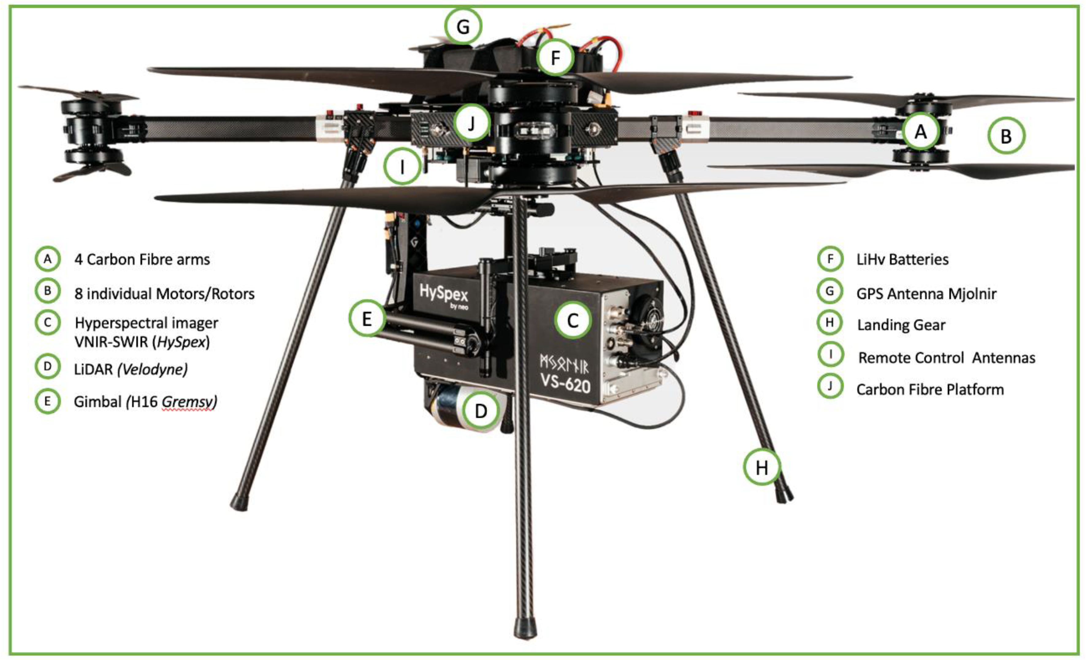
Figure 2.
UAS flying the payload of a hyperspectral imager (HySpex Mjolnir VS-620) and LiDAR. Total UAS is below 25kg, size motor to motor 140cm.
Figure 2.
UAS flying the payload of a hyperspectral imager (HySpex Mjolnir VS-620) and LiDAR. Total UAS is below 25kg, size motor to motor 140cm.
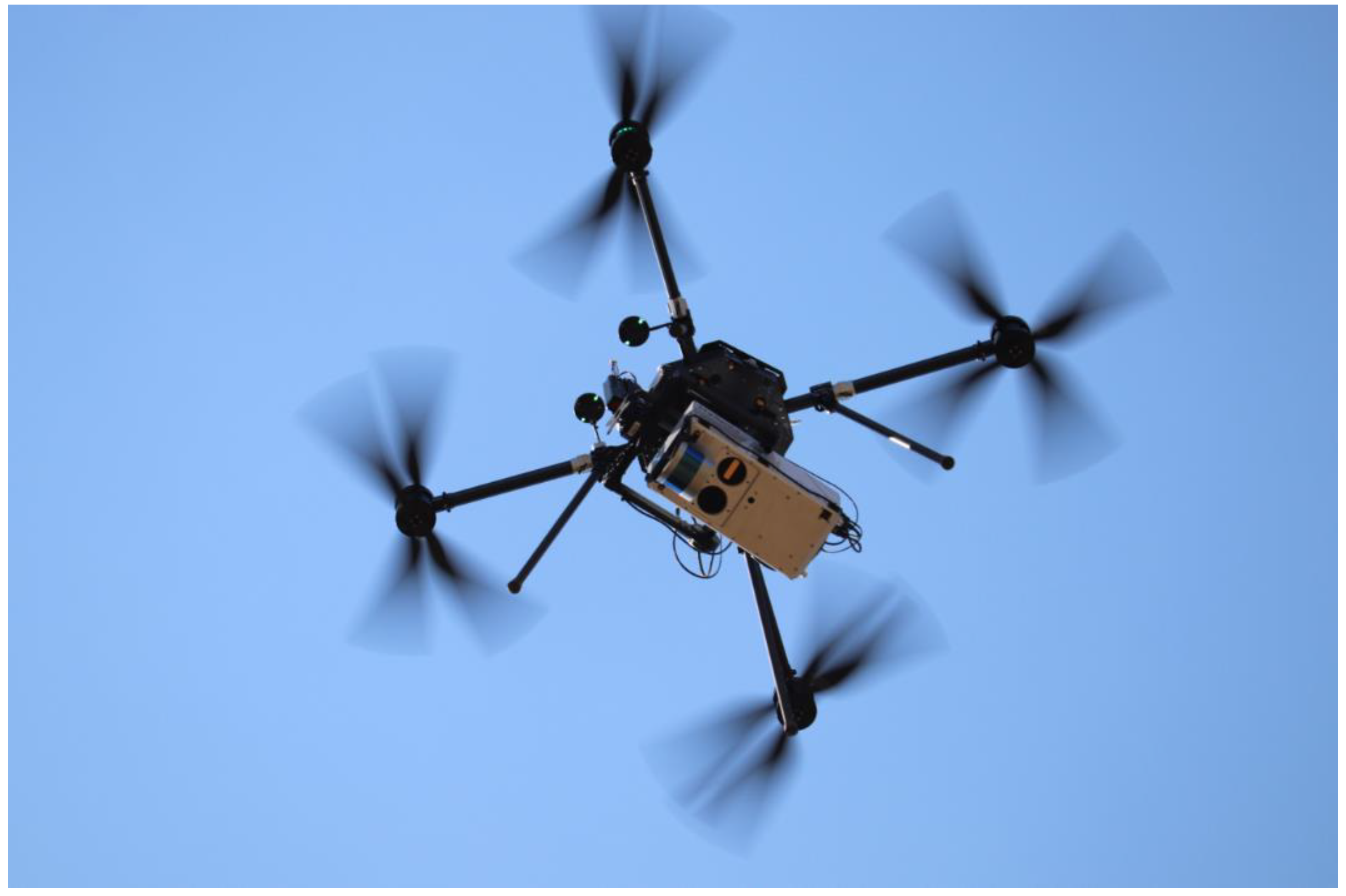
Figure 3.
Sampling points marked in recent M4Mining (www.m4mining.eu) UAV campaign in Queensland, Australia. Right: Sampling areas are marked via 50x50cm outline using white chalk spray. Only the sample’s immediate surface is sampled. Left: Location of the 50x50cm marker in the ca. 12x12 cm pixel resolution drone data captured by HySpex Mjolnir-VS620.
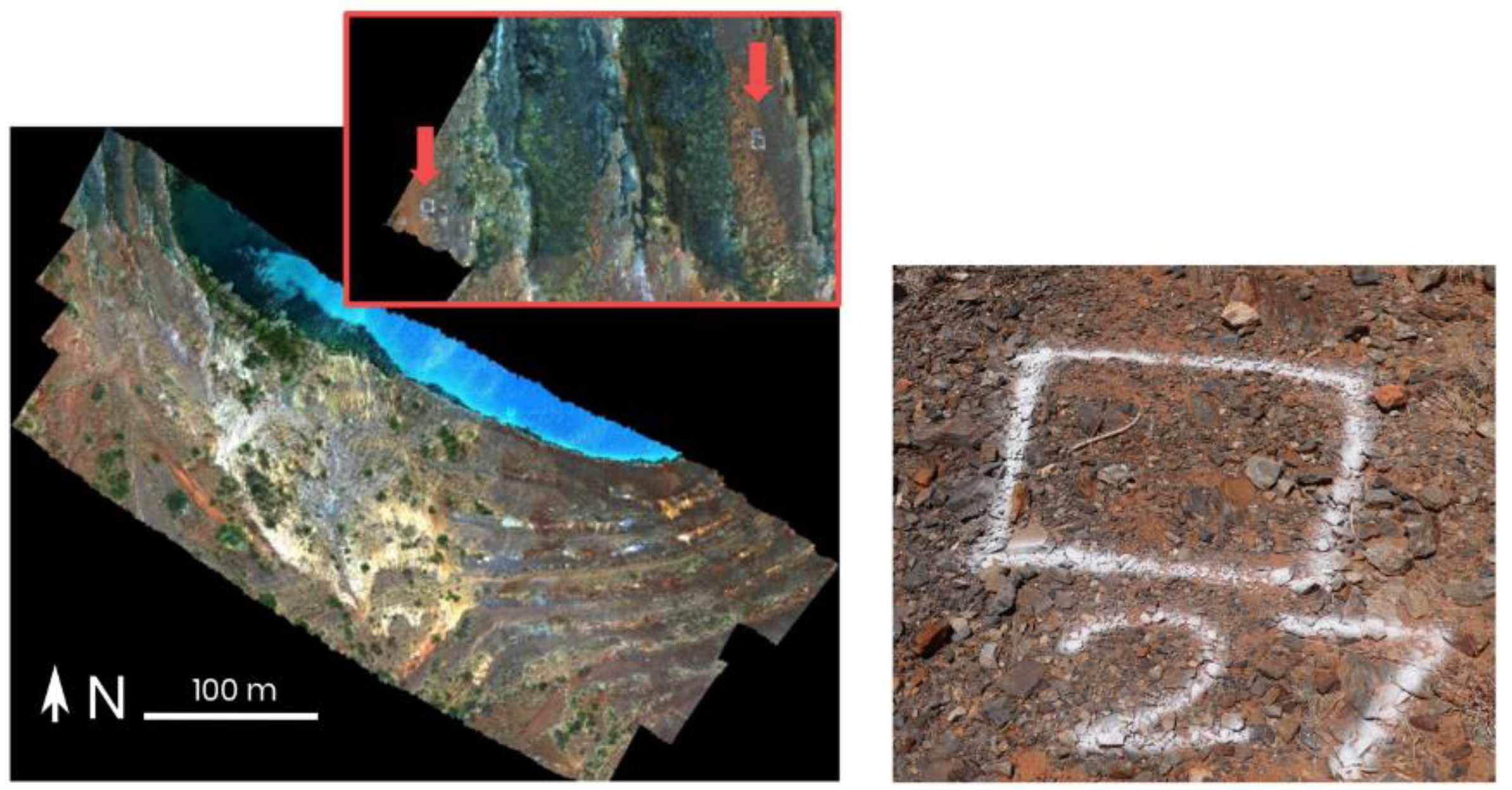
Figure 4.
D mineral models of Rocklea Dome area [124]. Scene centre is approximately lat 22.8216∘, long 117.4652∘. (a) (A) is showing the kaolin disorder index based on reflectance data from airborne HyMap™ (surface) and drill core HyLogger™ (coloured vertical pegs). Warmer colours (well-ordered kaolin) indicate the position of weathered, in situ bedrock, while to transported (alluvium/colluvium) materials are shown in cooler colours (poorly ordered kaolin). The interpolated model of the base of the channel iron system is shown by the shaded grey surface. The CID, which was calculated from the XRF-derived weight percent FeO [125], is shown by a shaded red volume (C). Areas of weathered bedrock [124,126] are highlighted by yellow-coloured hashed lines and highlight which drill cores were sunk into barren ground (D, E, F, G). A straight white line shows the location of the cross section (A–B) presented in panel (b). (b) Cross section A–B of the % FeO measured from the drill core and airborne imagery [127]. Dotted orange polygon indicates the shell of iron ore, which extends from under cover of ∼ 20 m of alluvium (H) to exposed at the surface (I). Figure from [100] published open access (https://creativecommons.org/licenses/by/4.0/). Please refer to [100] for in detailed descriptions of the derived and presented indeces.
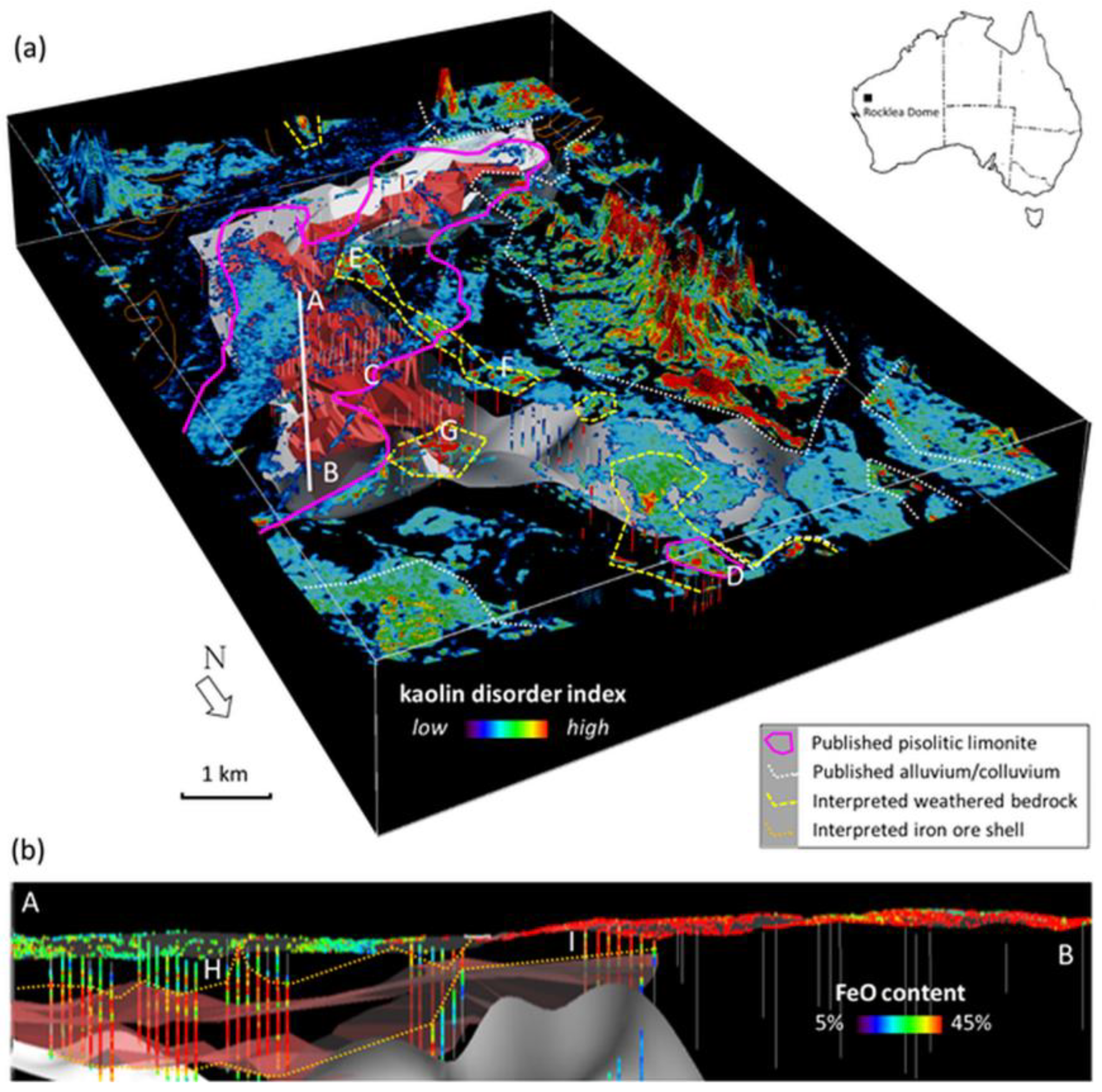
Figure 5.
Outcrop scale mineral map using HSI data collected by the U.S. Geological Survey personnel in the Cresson pit. Figure from [154] published open access (https://creativecommons.org/licenses/by/4.0/).
Figure 5.
Outcrop scale mineral map using HSI data collected by the U.S. Geological Survey personnel in the Cresson pit. Figure from [154] published open access (https://creativecommons.org/licenses/by/4.0/).
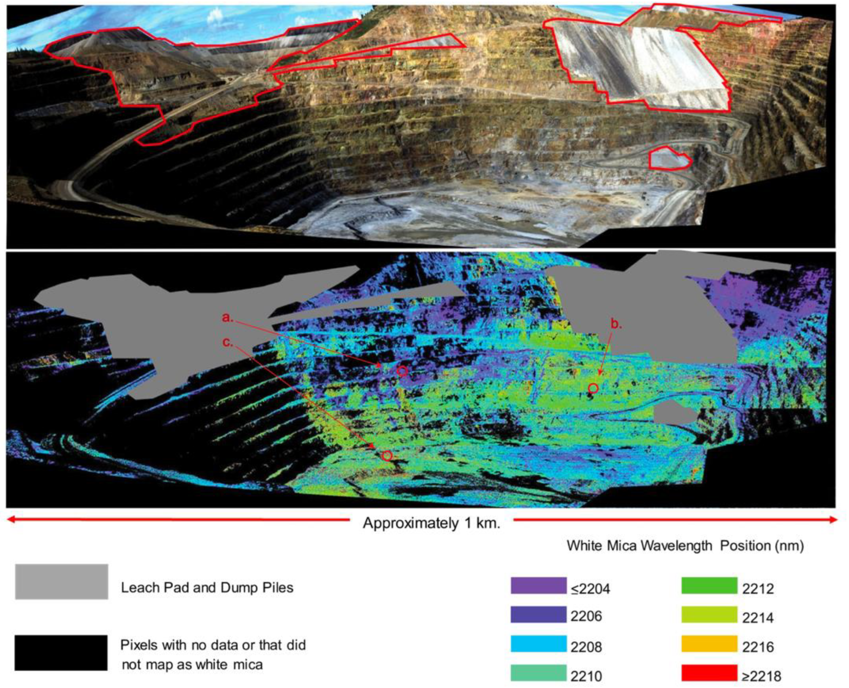
Figure 6.
Fe(III) iron band ratio indices for simulated Sentinel-2 (a), PlanetScope 2.SD (b), UAV (c) and ASD Halo handheld spectrometer (d) and a natural RGB image of Wheal Maid. Red areas indicate high Fe(III) iron pixel distribution, dark green areas denote vegetated areas. A model for the handheld point spectrometer is created via kriging (d). Figure from [60], published open access (https://creativecommons.org/licenses/by/4.0/. Graphs (f)-(h) were clipped out from the original figure.
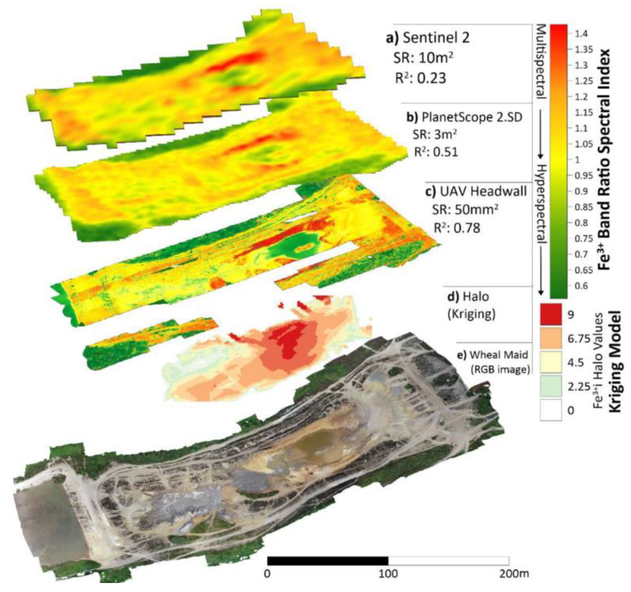
Figure 7.
The spatial distribution of ferric iron oxides surrounding the Chuquicamata porphyry copper mine in Chile using EnMAP hyperspectral satellite data acquired on 30.04.2023. The left panel displays natural colour composite imagery, the middle panel illustrates the relative abundance of ferric iron oxides, and the right panel shows the minimum wavelength of the ferric feature from 875nm to 955nm. This wavelength range indicates the prevalence of jarosite (blueish) and goethite (reddish) within the regions. This data has been prepared within the M4Mining project to demonstrate EnMap mapping capabilities in large-scale mining environments. Mapped patterns are purely based on satellite data and have not been validated on site.
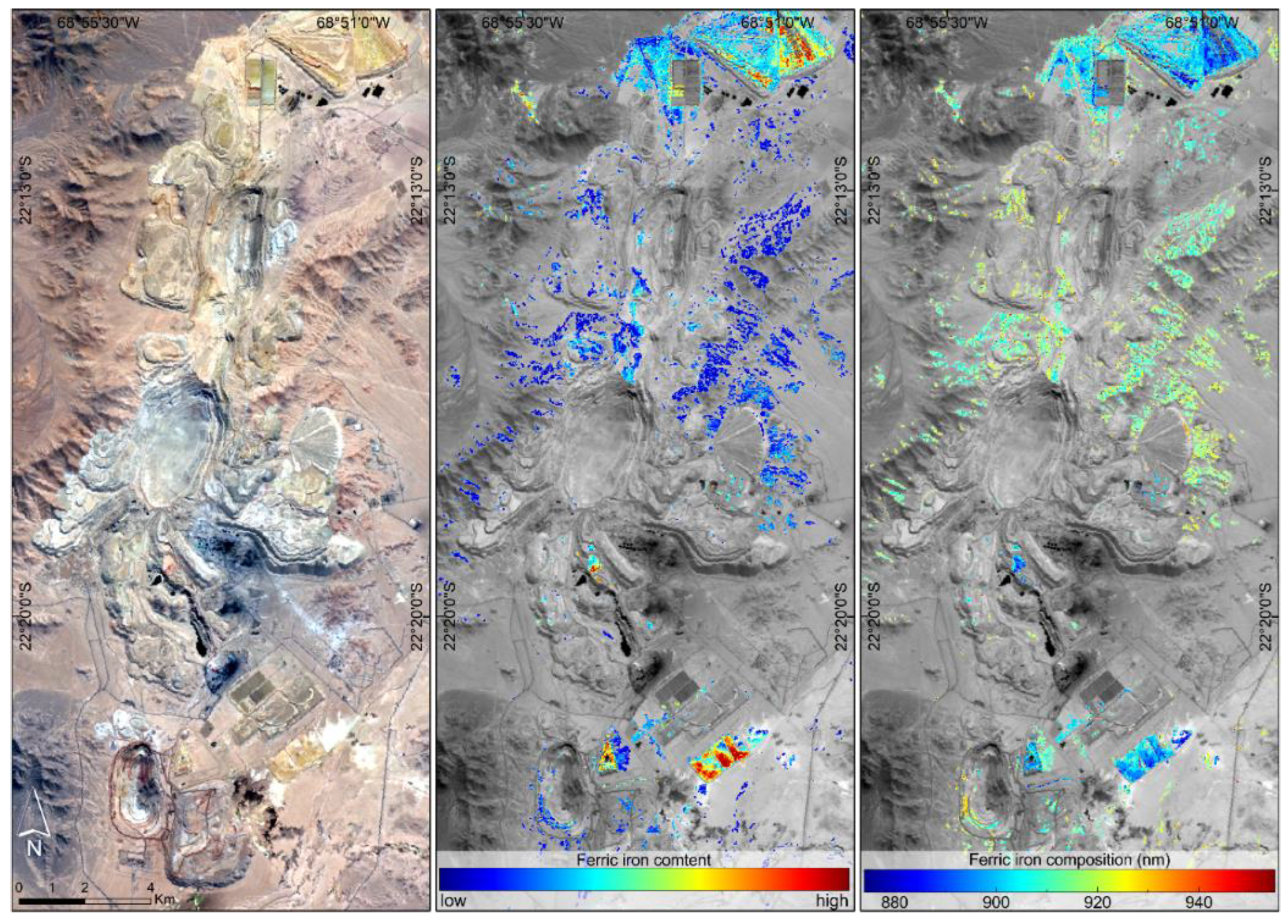
Figure 8.
Graphical abstract from Flores et al. (2021), showing results of the random forest regression predictions for pH values in the river water. Figure available via CC BY 4.0 licensing (https://creativecommons.org/licenses/by/4.0).
Figure 8.
Graphical abstract from Flores et al. (2021), showing results of the random forest regression predictions for pH values in the river water. Figure available via CC BY 4.0 licensing (https://creativecommons.org/licenses/by/4.0).
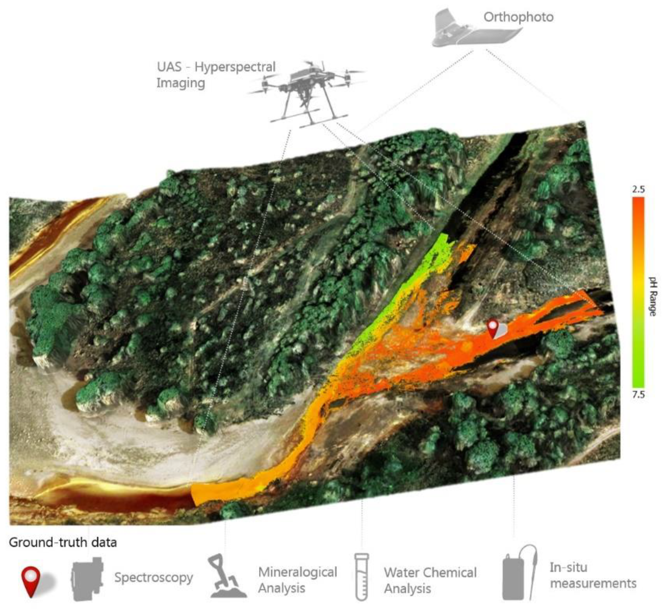
Figure 9.
Secondary iron mineral maps from the Skouriotissa mine monitoring for acid-forming potential. Left: Mineral mapping based on WorldView-2 data provided by European Space Imaging® within the ESA TPM project 61058 (4m x 4m pixels); Right: Mineral map based on Copernicus Sentinel-2 data (20m x 20m pixels). From [183] licensed under CC BY 4.0 (https://creativecommons.org/licenses/by/4.0/).
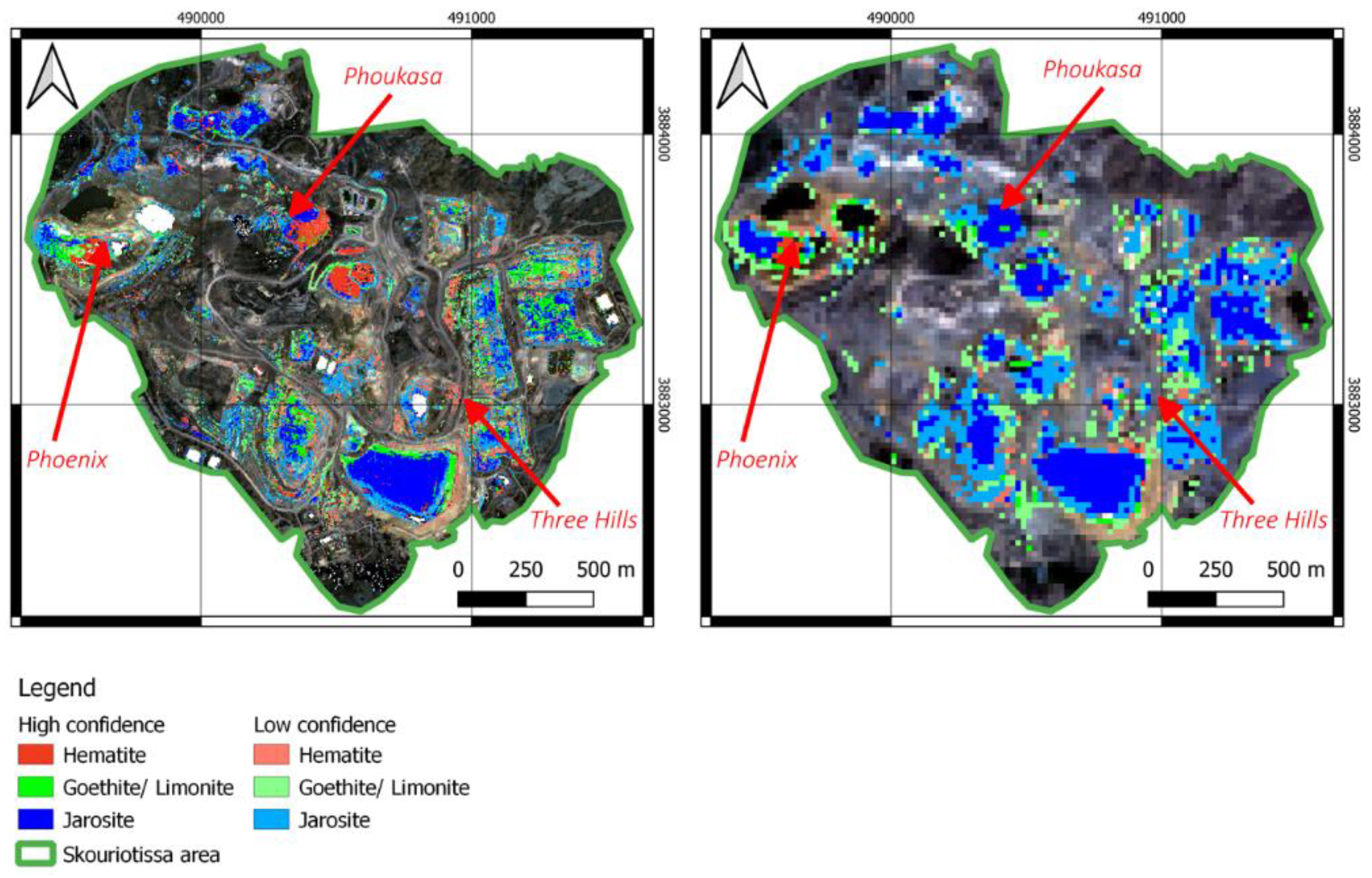
Table 1.
Currently available off-the-shelf hyperspectral cameras that can or have been mounted to a UAS platform. The list is based on freely available information collected during April 2024. The authors cannot guarantee that information on hardware provider’s websites is up-to-date or complete.
Table 1.
Currently available off-the-shelf hyperspectral cameras that can or have been mounted to a UAS platform. The list is based on freely available information collected during April 2024. The authors cannot guarantee that information on hardware provider’s websites is up-to-date or complete.
| Name (Service provider/ brand/ name of instrument) | Wavelength range | Type of data acquisition | Spectral bands and sampling |
| NEO/HySpex Mjolnir VS-620 |
VNIR (400 – 1000 nm) SWIR (970 – 2500 nm) |
Pushbroom | 200 bands @ 3nm; 300 bands @ 5.1 nm |
| Headwall Nano HP | VNIR (400 – 1000 nm) | Pushbroom | 340 bands @ 1.76 nm |
| Headwall Micro 640 | SWIR (900 – 2500 nm) | Pushbroom | 267 bands @ 6 nm |
| Headwall Co-Aligned HP | VNIR (400 – 1000 nm) SWIR (900 – 2500 nm |
Pushbroom | 340 bands @ 1.76nm; 267 bands @ 6 nm |
| Senop Rikola | VNIR (500 – 900 nm) | Frame-based snapshot | 50 bands @ 8 nm |
| Senop HSC-2 | VNIR (500 – 900 nm) | Frame-based snapshot | up to 1000 freely selectable bands @ 6 – 18 nm, |
| Specim AFX10 | VNIR (400 – 1000 nm) | Pushbroom | 224 bands @ 2.68 nm |
| Specim AFX17 | VIS-NIR (400 – 1700 nm) | Pushbroom | 224 bands @ 3.5 nm |
| Cubert GmbH ULTRIS X20 | UV-VNIR (350 – 1000 nm) | Snapshot | 164 bands @ 4 nm |
| Telops Hyper-Cam Nano (announced April 2024) | VIS – NIR (400 – 1700 nm) | - | - |
| Haip Solutions – Black Bird 2 | VNIR (500 – 1000 nm) | Hovering Linescanner | 100 bands @ 5 nm |
| Resonon Pika L | VNIR (400 – 1000 nm) | Pushbroom | 281 bands @ 2.7 nm |
| Resonon Pika IR-L | NIR (925 – 1700 nm | Pushbroom | 236 bands @ 5.9 nm |
| BaySpec OCI-UAV | VNIR (600 – 1000 nm) | Pushbroom and Snapshot | 100 bands @ 5 nm |
| IMEC | VNIR (460 – 900 nm) | Frame-based snapshot, multispectral | 31 bands |
Disclaimer/Publisher’s Note: The statements, opinions and data contained in all publications are solely those of the individual author(s) and contributor(s) and not of MDPI and/or the editor(s). MDPI and/or the editor(s) disclaim responsibility for any injury to people or property resulting from any ideas, methods, instructions or products referred to in the content. |
© 2024 by the authors. Licensee MDPI, Basel, Switzerland. This article is an open access article distributed under the terms and conditions of the Creative Commons Attribution (CC BY) license (http://creativecommons.org/licenses/by/4.0/).
Copyright: This open access article is published under a Creative Commons CC BY 4.0 license, which permit the free download, distribution, and reuse, provided that the author and preprint are cited in any reuse.


