
Submitted:
13 July 2024
Posted:
16 July 2024
You are already at the latest version
Abstract
Estimating the ocean’s subsurface thermohaline information from satellite measurements is essential for understanding ocean dynamics and El Niño phenomenon. This paper proposes an improved double-output Residual Neural Network (DO-ResNet) model to concurrently estimate the ocean subsurface temperature (OST) and ocean subsurface salinity (OSS) in the tropical Western Pacific using multi-source remote sensing data, including sea surface temperature (SST), sea surface salinity (SSS), sea surface height anomaly(SSHA), sea surface wind (SSW), and geographical information (including longitude (LON) and latitude (LAT)). In the model experiment, Argo data were used to train and validate the model, and the root mean square error (RMSE), normalized root mean square error (NRMSE) and coefficient of determination (R²) were employed to evaluate the model's performance. The results showed that the sea surface parameters selected in this study have a positive effect on the estimation process, and the average RMSE and R² values for estimating OST (OSS) by the proposed model are 0.34 °C (0.05 psu) and 0.91 (0.95), respectively. Under the data conditions considered in this study, DO-ResNet demonstrates superior performance relative to the extreme gradient boosting model, random forest model, and artificial neural network model. Additionally, this study evaluates the model’s accuracy by comparing its estimations of OST and OSS across different depths with Argo-derived data, demonstrating the model's ability to effectively capture the most spatial features, and by comparing NRMSE across different depths and seasons, the model displays strong seasonal adaptability. In conclusion, this research introduces a novel artificial intelligence technique for estimating OST and OSS in the tropical Western Pacific Ocean.
Keywords:
AI oceanography
; machine learning
; ocean thermohaline structure
; remote sensing data
; tropical Western Pacific
1. Introduction
Ocean temperature and salinity are two key parameters of seawater, playing significant roles in understanding marine ecosystems, ocean dynamics, and climate change. For instance, changes in ocean temperature can influence various oceanic phenomena, such as marine heatwaves, thermocline formation, and the evolution of El Niño [1,2,3]; meanwhile, variations in ocean salinity are crucial for understanding the characteristics of the hydrological cycle, ocean circulation, and water mass formation [4,5,6]. Therefore, accurately estimating the ocean subsurface temperature (OST) and ocean subsurface salinity (OSS) is vital for comprehending ocean dynamics, climate change, and predicting future climate scenarios.
The estimation of the OST and OSS was traditionally based on numerical simulations, data assimilation, dynamical models, and statistical models [7,8,9,10,11]. For instance, Wan et al. [12] analyzed the performance of two data assimilation methods, the ensemble Kalman filter and ensemble optimal interpolation, via Hybrid Coordinate Ocean Model for accurately predicting temperature and salinity in the Pacific system. The accuracy of dynamic ocean model heavily relies on observational data as input. However, the spatiotemporal data provided by in situ observations are often sparse and discontinuous, leading to the omission of some complex ocean dynamic processes [13], thereby affecting the estimation of subsurface temperature and salinity structures. As a result, classical methods face challenges such as limited spatial coverage, low spatiotemporal resolution, and reduced accuracy.
Over the past few decades, with the rapid development of remote sensing technology, continuous and extensive sea surface data, such as sea surface temperature (SST), sea surface salinity (SSS), and sea surface height (SSH) have been accumulated. Many studies have demonstrated that subsurface properties can be characterized by related surface parameters [14]. For example, Chu et al. [15] demonstrated that ocean interior temperature structure is closely related to SST and showed that SST can be used to estimate the OST. Consequently, many researchers have combined ocean surface data with methods such as linear regression [16], least-squares regression [17,18], and empirical orthogonal functions (EOF) [19,20] to retrieve the three-dimensional structure of the ocean interior. For instance, Guinehut et al. [21] utilized satellite altimeter data and sea surface observations to derive global temperature and salinity fields through linear regression methods. Similarly, Maes et al. [22] reconstructed the subsurface salinity structure of the tropical Western Pacific by employing EOF with SSH and SST data. Although observational data provides continuous and extensive samplings, traditional methods such as data assimilation and numerical simulations of subsurface ocean variables remain complex, computationally intensive, and may not guarantee high estimation accuracy.
In recent years, data-driven artificial intelligence (AI) models have attracted significant attention in the field of oceanography. These models effectively explore latent relationships within the data and estimate the internal physical structure of the ocean based on various observational datasets [23,24,25,26]. Early studies have employed machine learning models to retrieve the ocean's internal structure from multi-source surface data. For example, Ali et al. [27] utilized artificial neural networks (ANN) to reconstruct the vertical temperature profile of the Arabian Sea based on surface ocean data, including SST, SSH, wind stress, net radiation, and net heat flux. In another study, Wu et al. [28] integrated the self-organizing map (SOM) neural network algorithm with various satellite remote sensing datasets to reconstruct the subsurface temperature profile of the North Atlantic, demonstrating their model's superiority over traditional methods. Given the spatial correlation of data, Chen et al. [29] combined EOF analysis with SOM method to estimate the subsurface temperature structure of the Northwest Pacific using sea surface data. EOF analysis simplifies and decomposes complex spatial data structures, while the SOM method captures nonlinear relationships within the data. The integration of these two methods is better suited for describing the nonlinear dynamic processes in the ocean. Additionally, Dong et al. [30] proposed a light gradient boosting machine-deep forest method to estimate the OSS of the South China Sea, showcasing the potential of this approach in OSS estimation. Su et al. [31,32,33] used various satellite sources data to estimate global ocean subsurface temperature anomalies (STAs) with machine learning methods such as the random forest (RF), the support vector regression, and other artificial intelligence methods. They also applied the extreme gradient boosting (XGBoost) model to estimate anomalies in both subsurface temperature and salinity across the global ocean [34].
In addition to the machine learning models mentioned above, more and more deep learning models have been used to estimate OST and OSS. Meng et al. [35] designed a deep neural network model based on convolutional neural networks (CNN), utilizing multi-source satellite sea surface data to estimate the STA and subsurface salinity anomalies in the Pacific at a higher spatial resolution, significantly improving the resolution and accuracy of satellite observations in estimating internal oceanic parameters. Furthermore, Su et al. [36] combined sea surface remote sensing observations and Argo gridded data to propose a bi-directional long short-term memory neural network method for predicting global ocean STA and subsurface salinity anomalies, effectively learning significant temporal features of ocean variability and enhancing the generalization capability of the prediction model. Cheng et al. [37] utilized the backpropagation neural network method to determine the OST in the North Pacific using SSH, SST, SSS, sea surface wind (SSW), and sea surface velocity obtained from remote sensing satellites. Mao et al. [38] proposed a dual-path convolutional neural networks (DP-CNN) to reconstruct the OST and OSS structures in the South China Sea using sea surface information, demonstrating that DP-CNNs effectively reduce the issue of detail loss in CNN models. These AI-based research methods provide new avenues for the estimation of OST and OSS.
Existing AI models have shown the capability to estimate OST and OSS in many regions; however, the tropical Western Pacific region is less documented. Additionally, their computational accuracy still requires improvement, especially in regions with complex dynamic processes. For instance, Wang et al. [39] proposed an enhanced ANN model based on multi-source sea surface data to estimate OST in the Western Pacific. However, the model's average root mean square error (RMSE) value reached as high as 0.55 . This lack of precision may stem from the model's limited capacity to extract and learn spatiotemporal features of complex nonlinear systems. Therefore, there is considerable potential for improvement in both the model itself and its accuracy.
Motivated by the aforementioned discussions, the primary objective of this study is to develop a novel method based on multi-source remote sensing data to estimate the OST and OSS simultaneously in regions with complex dynamic processes. Consequently, this study proposes a new estimation method using the double-output Residual Network (DO-ResNet) model, aiming to utilize multiple satellite remote sensing data, including SST, SSS, sea surface height anomalies (SSHA), SSW, and geographic information, to estimate thermohaline structure in the tropical Western Pacific. Additionally, a series of estimation models are introduced for comparison in order to evaluate the proposed model. The remainder of this paper is organized as follows: Section 2 describes the study area and data, detailing the importance of the area studied and the multi-source remote sensing datasets used in the research. Section 3 outlines the research methods, describing the construction and training process of the DO-ResNet model. Section 4 presents the research results, exhibiting the OST and OSS estimated by the DO-ResNet model, and assesses the model's performance and accuracy through error statistics and comparative analysis. Section 5 summarizes and discusses the research findings, outlining the main discoveries and contributions, and explores the limitations of the methods as well as directions for future research.
2. Study Area and Data
2.1. Study Area
The strong El Niño event occurred in the Central and Eastern Pacific, significantly impacting the global climate [40,41]. As research has progressed, the scope of El Niño studies has gradually expanded to the tropical Western Pacific region (Figure 1). As the region with the highest sea surface temperatures globally, the tropical Western Pacific contains the largest and warmest body of water in the world [42]. Many scholars have found that variations in temperature and salinity in the tropical Western Pacific critically impact regional oceanic phenomena such as tropical cyclones, El Niño-Southern Oscillation (ENSO) events, the Pacific Decadal Oscillation, and monsoon variations [43,44,45,46]. However, due to a lack of observations, our understanding of the spatiotemporal variations in temperature and salinity in the tropical Western Pacific remains limited, significantly constraining research on the thermohaline structure of this region. Therefore, accurately estimating OST and OSS in the tropical Western Pacific is crucial for understanding the variability of ocean-atmosphere heat fluxes and analyzing the dynamic mechanisms of oceanic phenomena in this area.
2.2. Data Source and Preprocessing
The dataset for this study includes a series of sea surface remote sensing data and RG-Argo gridded data for the tropical Western Pacific region, spanning from January 2010 to December 2020, as summarized in Table 1. The monthly SSS data utilized in this study are derived from the Soil Moisture and Ocean Salinity (SMOS) Level-3 product [47], featuring a spatial resolution of . The monthly SST data are sourced from the National Oceanic and Atmospheric Administration (NOAA) [48], comprising interpolated observations from satellite radiometers, with a spatial resolution of . The monthly SSHA data are obtained from the Archiving, Validation, and Interpretation of Satellite Oceanographic data (AVISO) project [49], with a spatial resolution of . The SSW data, encompassing both the northward component (USSW) and the eastward component (VSSW), are acquired from the Cross-Calibrated Multi-Platform (CCMP) product [50], with a spatial resolution of . To evaluate the model's performance, this study utilizes the Roemmich-Gilson Argo climatology (RG-Argo) gridded data [51], which serves as the label data with a spatial resolution of and comprises 58 standard depth levels ranging from 5 m to 1975 m. These data provide measurements of temperature, salinity, and other subsurface oceanographic parameters at each depth level. The datasets utilized in this study are detailed in Table 1.
To ensure the consistency and accuracy of the model, this study employs data spanning from January 2010 to December 2020. All datasets were processed into monthly averages and interpolated to a resolution of to guarantee uniform temporal and spatial coverage. Data points with missing parameters within the study region were excluded from the analysis. For the model input, each data point within the region was considered a central point, with the 81 data points within a grid surrounding the central point serving as a two-dimensional image representing that central point. Furthermore, to accelerate model convergence during training, all remote sensing and RG-Argo data were normalized using their respective means and standard deviations.
3. Methods
3.1. The DO-ResNet Model
Residual Neural Network (ResNet) [52] is a deep convolutional neural network architecture for handling complex image recognition and classification tasks in nonlinear case, which consist of multiple convolutional layers and residual blocks. Each residual block contains several convolutional layers and uses shortcut connections to add the original input to the output of the convolutional layers, thus preserving the information from the input data. Compared to traditional CNN, ResNet introduces shortcut connections while retaining the characteristics of CNNs, effectively addressing the vanishing gradient problem in deep neural networks and demonstrating exceptional intelligent characteristics. In recent years, people have applied ResNet in various fields to solve practical problems, such as drug-induced liver injury prediction [53], coral reef semantic segmentation [54], sea ice detection [55], and others [56,57].
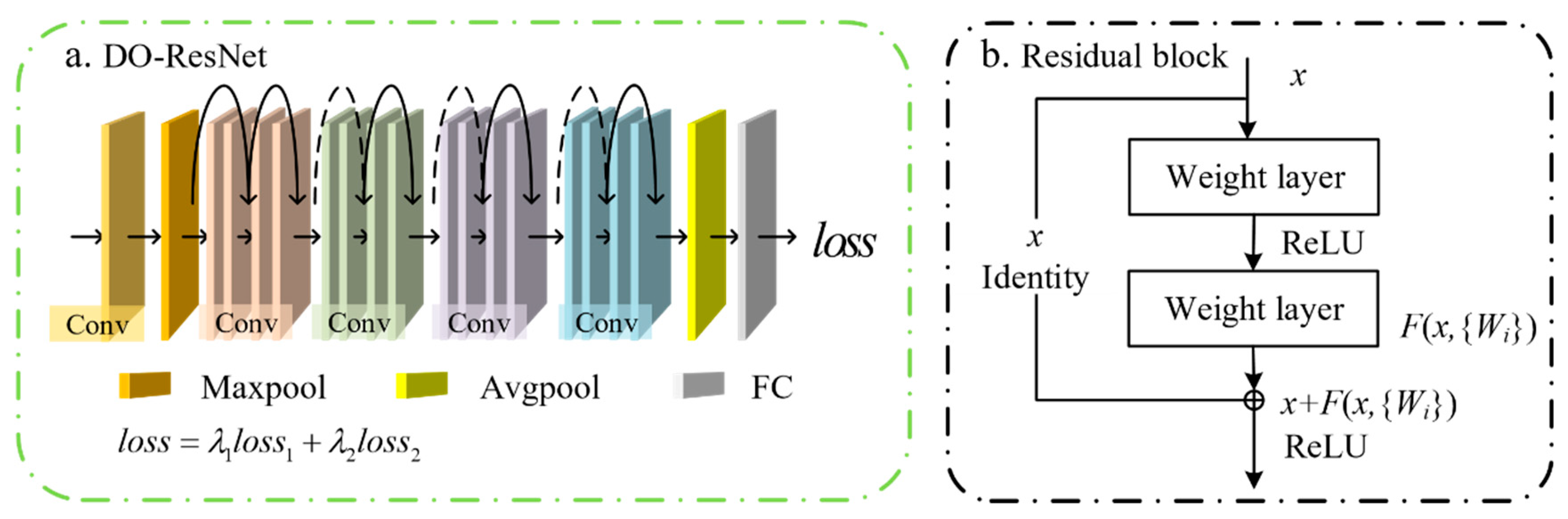
In view of a close relationship between the sea surface parameters and the subsurface thermohaline structure of the ocean, a double-output ResNet (DO-ResNet) model is proposed in this study, which can simultaneously estimate OST and OSS based on various sea surface parameters observed by satellites. The double-output design allows us to extract features of both temperature and salinity through a single model, resulting in two outputs and improving the model's efficiency. The structure of the improved DO-ResNet model is illustrated in Figure 2a. Firstly, the input data passes through a convolutional layer for preliminary feature extraction. This convolutional layer uses a 3×3 kernel, which effectively captures local features while reducing the impact of islands on the ocean temperature and salinity information at the ocean-island boundaries. Secondly, after deep feature extraction through the residual blocks, the data is flattened and fed into a fully connected layer for integration. Finally, the model estimates temperature and salinity through two independent output layers.
The structure of each residual block is shown in Figure 2b, consisting of two 3×3 convolutional layers, two Rectified Linear Unit (ReLU) [58] activation functions, and a shortcut connection. In each residual block, the input data x is processed sequentially through the first convolutional layer, the ReLU activation function, and the second convolutional layer to obtain the output . To preserve the original information of the input data, the input data x is directly connected to the output of the second convolutional layer via the shortcut connection. Finally, after passing through the ReLU activation function, the final output y of the residual block is generated. It is important to note that when the input and output dimensions are the same, the shortcut connection is represented by a solid line, and the propagation process is as described in Equation (1):
Here x and y are the input and output vectors of the layers considered. represents the learned residual mapping, where σ denotes the ReLU activation function. Similarly, shortcut connections that span feature maps of different dimensions are represented by dashed lines. In this case, a 1×1 convolutional layer is used to perform dimensionality upscaling on the input data x, and the propagation process is as described in Equation (2):
Here, x, y and have the same meanings as in Equation (1), and Ws represents the identity mapping obtained by processing the input x on the residual connection branch. This type of connection effectively reduces the loss of input information during propagation, preserves the integrity of the input data, and simultaneously lowers the risk of gradient vanishing, thereby enhancing the stability and performance of the neural network.
Figure 2.
The structure of DO-ResNet model, with the solid and dashed lines representing two different types of residual connections (a) and schematic diagram of shortcut connection in a residual block (b).
Figure 2.
The structure of DO-ResNet model, with the solid and dashed lines representing two different types of residual connections (a) and schematic diagram of shortcut connection in a residual block (b).
3.2. Experimental Setup
This study utilizes multi-source satellite observational data to develop a DO-ResNet model for estimating OST and OSS within the tropical Western Pacific region. The research workflow is illustrated in Figure 3 and is divided into three main stages. The first stage involves the collection and preprocessing of raw data. We collected five sea surface parameters: SST, SSS, SSHA, USSW, and VSSW as well as longitude (LON) and latitude (LAT) from multiple databases. These datasets were then preprocessed to create a training and testing dataset comprising gridded data points over 132 months. OST and OSS data derived from RG-Argo served as the training and testing labels. The second stage is model training. The monthly average data from January 2010 to December 2019 were used as training data to train the DO-ResNet model. During this phase, we selected the mean squared error (MSE) as the loss function. However, since the model simultaneously estimates both temperature and salinity, a composite loss function incorporating the MSE of these two variables is designed, as shown in Equation (3):
The coefficients and are weights that balance the contributions of the temperature and salinity losses. Based on the quasi-linear relationship between ocean temperature and salinity in the T-S diagram, we set both and to 0.5 [59]. By adjusting these weights, the overall performance of the model can be optimized. The and represent the MSE for the temperature and salinity estimates, respectively, with their calculation formulas given by Equations (4) and (5).
Here, and are the actual temperature and salinity values at the i-th data point, respectively, while and are the model-estimated temperature and salinity values at that data point. N is sample number. To prevent overfitting, random sampling of data points was employed, and a grid search method was used to identify the optimal parameter combination for the DO-ResNet model, as summarized in Table 2. The third stage is model testing. The test data from each month of 2020 were input into the model to obtain the prediction results. The performance of the DO-ResNet model was evaluated using RMSE and determination coefficient (R²). RMSE, which measures the difference between estimated and observed values, The R² metric is employed to evaluate the model's fitting performance, thereby assessing its estimation capability.
4. Results
4.1. Identification of Input Variable
A key issue in estimating OST and OSS in the tropical Western Pacific is the selection of model input variables. Previous studies have indicated that incorporating SSW and geographic information can enhance the accuracy of subsurface temperature and salinity estimations [36,60,61]. To further investigate the impact of SSW and geographic information on temperature and salinity estimations in this region, this study designed experiments with three different combinations of input parameters (Cases 1, 2, and 3) to compare the results estimated by DO-ResNet with different training inputs. Table 3 presents the parameter combinations for the three experimental cases. In Case 1, SSS, SST, and SSHA were selected as input parameters. In Case 2, both USSW and VSSW were added to these parameters. In Case 3, geographic information (LON and LAT) was added to the input parameters of Case 2.
Figure 4 shows the vertical distribution of RMSE and R2 for the three experimental cases. The results indicate that three experiments are able to estimate the vertical distribution of OST (OSS), with the main error centered on the depth of 150-200 m, which may be an effect of the thermocline [62]. However, the inclusion of SSW and geographic information in Case 3 improves the estimation accuracy of the DO-ResNet model in the tropical Western Pacific Ocean compared to Cases 1 and 2, as evidenced by smaller RMSE values and larger R2 values. Specifically, the vertically averaged RMSE and R2 for estimating the OST (OSS)were 0.51 (0.07 psu) and 0.84 (0.92) in Case 1, 0.46 (0.07 psu) and 0.87 (0.93) in Case 2, 0.35 (0.05 psu) and 0.91 (0.96) in Case 3, respectively. The DO-ResNet model in Case 3 exhibited significantly lower RMSE values across all depths compared to the results from Cases 2 and 1, and the R2 values were also notably higher. These results show that the DO-ResNet model for Case 3 can better fit the nonlinear relationship between the OST (OSS) in the tropical Western Pacific and the input parameters.
4.2. Accuracy Comparison between the DO-ResNet Model and Other Model
After determining the optimal parameter combination, this study compared the performance of the DO-ResNet model with three other models (XGBoost [34], RF [32], and ANN [39]) for estimating OST and OSS in the tropical Western Pacific using 2020 data. The parameter values for the models are detailed in Table 4.
Figure 5a,b illustrate the vertical distribution of RMSE and R2 for OST estimates by the four models. The findings reveal that the RMSE of OST estimates for all models increases from the sea surface, peaks around 200 m depth, and then decreases with further depth. In contrast, R2 values show an inverse pattern, decreasing from the surface to 200 m, peaking around 300 m, and then fluctuating. The DO-ResNet model outperforms the other models with consistently lower RMSE and higher R² values across various depths. For OSS estimates, shown in Figure 5c,d, a similar trend is observed: RMSE increases and then decreases, while R2 decreases initially peaks 750 m, and then gradually decreases. At depths of 150-200 m, the DO-ResNet model’s RMSE for OSS is relatively higher, and its R2 is relatively lower, possibly due to the thermocline, which complicates accurate estimation [62]. The model may struggle to capture the complex dynamics within this depth range. Despite this, the DO-ResNet model’s average RMSE and R² for OST (OSS) estimates across all depths is 0.35(0.06 psu) and 0.91 (0.96), while the overall average RMSE and R2 for XGBoost, RF, and ANN are 0.50 (0.07 psu) and 0.87 (0.93), 0.51 (0.06 psu) and 0.86 (0.93), and 0.43 (0.06 psu) and 0.90 (0.94), respectively. These results clearly illustrate that the DO-ResNet model surpasses the other models in performance, as evidenced by its smaller RMSE and higher R² values. Therefore, the DO-ResNet model is highly effective in accurately estimating OST and OSS in the tropical Western Pacific.
4.3. Vertical Performance Evaluation of the DO-ResNet Model
This section provides a comprehensive evaluation of the DO-ResNet model's performance in estimating OST and OSS from various perspectives. For a comprehensive assessment of the vertical performance of the DO-ResNet model, we analyzed two representative sections: a zonal section (section A) along the equator from to , and a meridional section (section B) along from to . The locations of these sections in the tropical Western Pacific are shown in Figure 1. The result is shown in Figure 6 and Figure 7.
) along zonal and meridional sections in 2020.
Figure 6a,b present the spatial distribution of OST along the zonal section A as observed by Argo and estimated by the DO-ResNet model, respectively. Similarly, Figure 6d,e display the vertical distribution of OST along the section B. The DO-ResNet model exhibits strong agreement with the Argo observations, accurately capturing the vertical distribution of OST. The 20 isotherm highlights a pronounced vertical gradient in both observed and estimated temperatures at the surface and within the thermocline, consistent with findings from previous studies regarding thermocline depth [63]. From the surface to the thermocline depth, seawater temperature decreases rapidly. Beyond the thermocline, the temperature decline is more gradual, reaching a stable state at depths below 500 m.
Figure 6c and Figure 6f displays the difference between the Argo observations and the DO-ResNet model estimates of OST along section (Argo observations minus DO-ResNet estimates). The differences are generally minor, with more significant discrepancies primarily in the shallow layers. For instance, for section A, at depths shallower than 300 m between 130 and 160, the model estimates are approximately 0.8 lower than the observations, while between 160 and 150, there are regions where the model estimates are higher than the observations. Similarly, Figure 6f shows that larger differences (exceeding 0.5 ) are primarily located in the shallow layers (50-500 m), likely due to the complex circulation system in the equatorial Pacific region [64].
Similarly, the DO-ResNet model's estimates of OSS align well with Argo observations along both zonal and meridional sections, effectively reproducing the distribution characteristics of OSS. Figure 7a,b illustrate the vertical distribution of OSS along the zonal section, while Figure 7c depicts the differences between Argo observations and the DO-ResNet estimates. In the upper ocean layers, specifically between 50 and 100 m, the maximum salinity difference in certain regions (130 to 150) reaches 0.23 psu, which may be influenced by the New Guinea Island and Maluku Islands. As depth increases, the DO-ResNet model's estimated OSS stabilizes, with the difference between the estimated and observed salinity being less than 0.14 psu. Similarly, Figure 7d,e show the vertical distribution of OSS along the meridional section, while Figure 7f shows the differences between the two. With increasing depth, the discrepancies between the DO-ResNet model's estimates and the Argo observations along the meridional section gradually decrease. These results confirm the effectiveness of the DO-ResNet model in estimating OSS in the tropical Western Pacific.
To evaluate the performance of the DO-ResNet model at different depths, Figure 8 and Figure 9 present the annual mean OST and OSS at six different depths (50 m, 200 m, 500 m, 1000 m, 1500 m, and 1900 m) estimated by the DO-ResNet model for 2020. The model’s performance is evaluated by comparing the differences between the Argo data and the DO-ResNet estimates.
Figure 8 shows the spatial distribution of OST estimated by the DO-ResNet model at various depths, demonstrating a high degree of consistency with the observed OST. At 50 m depth, Argo observations indicate that the highest temperatures in the tropical Western Pacific occur at the equator, with sea surface temperatures gradually decreasing towards both poles, and a distinct thermal front appearing near . The DO-ResNet model accurately captures this significant thermal feature. At 200 m depth, the differences between the DO-ResNet model's estimated OST and the Argo observed OST range from to 1.55 , which is greater than the differences at 50 m depth, likely due to the thermocline’s influence. As depth increases, the temperature stabilizes, and below 1000 m, the differences between the temperatures from Argo data and DO-ResNet model estimates are minimal, ranging from to 0.26 . These results confirm that the DO-ResNet model is highly accurate in estimating OST in the tropical Western Pacific.
Similarly, Figure 9 illustrates the spatial distribution of OSS estimated by the DO-ResNet model in comparison with Argo observations. The results reveal that the OSS values estimated by the DO-ResNet model show a high degree of consistency with the Argo observations, effectively reproducing the distribution characteristics of OSS. In the upper ocean layers (50 m and 200 m), the salinity differences across most regions range from psu to 0.26 psu. As depth increases, OSS becomes more stable, and the differences between the salinity estimated by the DO-ResNet model and that provided by Argo are less than 0.1 psu. These findings confirm the reliability of the DO-ResNet model for estimating OSS in the tropical Western Pacific.
) from Argo observation (a-f) and DO-ResNet estimation (g-l) and their differences (Argo observations minus DO-ResNet estimates, m-r) at different depths (50 m, 200 m, 500 m, 1000 m, 1500 m and 1900 m) in 2020.
4.4. Seasonal Performance of the DO-ResNet Model
In this section, the months of February, May, August, and November of 2020 have been chosen to represent winter, spring, summer, and autumn, respectively, to investigate the model's performance across different seasons. The model’s performance was evaluated at 22 different depths (ranging from 30 m to 1900 m) across these four seasons. To ensure comparability across depths, the RMSE values were divided by the standard deviation of the Argo temperature and salinity values at each depth, resulting in the NRMSE. The NRMSE and R2 values for different seasons and depths are illustrated in Figure 10.
Figure 10a presents the vertical distribution of NRMSE and R2 values of the OST estimated by the DO-ResNet model across different seasons and depths. The NRMSE across different seasons exhibits a downward trend followed by an upward trend, with a turning point occurring at depths of approximately 200 to 400 m. Beyond 600 m, NRMSE rises with depth slowly, reflecting the model’s weaker performance in deeper layers, making it harder to estimate deeper phenomena with surface data. Additionally, the higher NRMSE values at depths shallower than 100 m could be related to the complex dynamic processes occurring in the upper ocean. This pattern is consistent with previous studies on model-estimated OST in other regions [65]. The DO-ResNet model demonstrates robust performance in estimating OST across different seasons. The maximum NRMSE values for February and May are 0.40 and 0.42, respectively, while for August and November, they are 0.40 and 0.39, respectively, indicating better model performance in winter. The estimation accuracy of the DO-ResNet model varies with the seasons. Average NRMSE (R2) values for February, August, and November are 0.30 (0.91), 0.32 (0.90), and 0.31 (0.90), respectively, while May has the highest average NRMSE of 0.34 and the lowest average R2 of 0.88 among the four seasons, indicating poorer estimation accuracy in summer. The figure also shows higher NRMSE values at most in summer compared to other seasons.
Figure 10b illustrates the distribution of NRMSE and R2 for the model-estimated OSS across different seasons and depths. The NRMSE values show an increasing trend from the sea surface to 100 m, then level off between 200 m and 1200 m, and increase again at depths greater than 1200 m. This reflects that the DO-ResNet model is able to effectively estimate subsurface salinity in the 1200 m depth layer based on surface data obtained from remote sensing, but its accuracy in estimating salinity at deeper depths is reduced. From the figure, it can be seen that the maximum NRMSE values for February and August occur around a depth of 70 m, being 0.42 and 0.35, respectively, while for May and November, the maximum values are 0.36 and 0.39, respectively. This indicates that the DO-ResNet model has larger errors in spring and autumn at 70 m, which may be affected by seasonal changes in freshwater fluxes [66] and the thermocline [67]. In general, the seasons had similar vertically averaged NRMSE and R2, with NRMSE around 0.22 and R2 around 0.94, which suggests that the DO-ResNet model is less seasonally influenced and robust in estimating OSS.
4.5. Correlation Analysis between the OST (OSS) and Surface Parameters
In order to evaluate how sea surface parameters influence the performance of the DO-ResNet model, we determined the Pearson correlation coefficients between SST, SSS, SSHA, USSW, and VSSW and the OST and OSS at various depths (50 m, 60m, 100m, 200 m, 500 m, 1000 m, 1500m, and 1900m) presented in Figure 11. A higher absolute value of the Pearson correlation coefficient indicates a greater influence of the sea surface parameter on the estimation of OST or OSS. By comparing these coefficients, we can determine the significance of each parameter in the model’s estimation of OST and OSS at different depths.
Figure 11a illustrates the Pearson correlation coefficients between sea surface parameters and the estimated OST. It is evident that SST and SSHA exhibit a strong correlation with OST. Specifically, SST has the highest correlation with OST at 50 m, with a coefficient of 0.86, while SSHA shows the highest correlation at 100 m, with a coefficient of 0.63. In contrast, USSW and VSSW display a weaker correlation with OST, with most coefficients being less than 0.33. SSS significantly impacts OST in the shallow layers, but its correlation diminishes with depth, reaching a minimum coefficient of 0.31 at 1000 m. Beyond 1000 m, its correlation is comparable to that of USSW and VSSW.
Figure 11b shows the correlation of various sea surface parameters with the DO-ResNet model's estimates of OSS at different depths. The results indicate that SSS, SST, and SSHA have significant impacts on OSS estimation. Specifically, SSS exhibits a high correlation with OSS in the surface layer, with a correlation coefficient of 0.51 at 50 m. However, its correlation weakens in the deeper ocean, reaching approximately 0.31. SST and SSHA maintain correlation coefficients above 0.4 at most depths, indicating their considerable and stable influence on OSS estimation across different depth ranges. In contrast, USSW and VSSW exhibit weaker correlations with OSS. Nevertheless, these parameters still contribute to OSS estimation and should not be disregarded in the estimation process. The analysis indicates that the selected sea surface parameters are effective variables for estimating both OST and OSS.
5. Discussion
As the region with the highest sea surface temperatures globally, the tropical Western Pacific exhibits significant climate signals across various time scales. Its temperature and salinity demonstrate variations on interannual and decadal scales associated with major climate patterns such as the ENSO and the Pacific Decadal Oscillation. Accurately estimating the vertical structure of three-dimensional temperature and salinity fields in the tropical Western Pacific is crucial for understanding oceanic processes and climate change. However, due to the challenges and high costs associated with in situ observations, temperature and salinity data in the tropical Western Pacific remain sparse. This study introduces an improved DO-ResNet model, utilizing satellite-derived sea surface data (SSS, SST, SSHA, and SSW) and geographic information (longitude and latitude) as input, with Argo data employed as the ground truth for training and validation. The model reconstructs OST and OSS in the tropical Western Pacific. The accuracy and reliability of the DO-ResNet model's estimates are assessed using RMSE, NRMSE, and R2 metrics. Furthermore, the model's performance is evaluated from various perspectives, including spatial distribution, vertical sections, and seasonal variations.
This study evaluates the accuracy of the DO-ResNet model in estimating OST and OSS by comparing its output at various depths with observational data from Argo floats. Results indicate that the optimized composite loss function enables the DO-ResNet model to effectively reconstruct most observed features of OST and OSS concurrently in the tropical Western Pacific. However, due to the presence of the thermocline, the estimation accuracy of OST and OSS is lower at depths around 150-200 m, posing challenges for accurately estimating the three-dimensional temperature and salinity fields near this depth. Despite this, the overall performance of the DO-ResNet model is commendable, with the average RMSE and R2 for OST (OSS) being 0.34 (0.05 psu) and 0.91 (0.95), respectively. Furthermore, this study evaluates the impact of sea surface parameters on the performance of the DO-ResNet model, indicating that sea surface variables play a more significant role in the upper ocean, particularly in shallow layers. SST and SSHA are crucial for estimating OST, while SSS, SST, and SSHA are key for estimating OSS. Moreover, the model exhibits low NRMSE and high R² values across all seasons, indicating its robust seasonal applicability for OST and OSS estimation in the tropical Western Pacific.
In summary, the DO-ResNet model demonstrates superior performance in estimating OST and OSS in the tropical Western Pacific. The model exhibits high estimation accuracy for OST and OSS across different depths and seasons. The results of this study are significant for understanding the subsurface information of the tropical Western Pacific in the context of ENSO occurrence and provide a foundation for further research into the ENSO mechanisms in the tropical Western Pacific. Future research should focus on employing more advanced artificial intelligence methods and integrating ocean dynamic mechanisms to further enhance estimation accuracy. Additionally, the application of this model can be extended to broader oceanic regions, allowing for precise estimation of OST and OSS, and facilitating practical applications such as mixed layer depth estimation and ocean hazard prediction. Moreover, the model can be further utilized to estimate other critical ocean parameters, such as velocity fields and ocean density, thus opening up new avenues for future research.
Author Contributions
Conceptualization, S.Z.; methodology, X.Z.; software, X.Z. and W.J.; validation, S.Z., W.J. and H.Y.; formal analysis, X.Z. and H.Y.; investigation, X.Z. and W.J.; resources, S.Z. and H.Y.; data curation, S.Z. and H.Y.; writing—original draft preparation, X.Z., H.Y. and W.J.; writing—review and editing, H.Y., S.Z., X.Z. and W.J.; visualization, X.Z., S.Z. and H.Y.; supervision, S.Z. and H.Y.; project administration, S.Z. and H.Y.; funding acquisition, H.Y. All authors have read and agreed to the published version of the manuscript.
Funding
This research received no external funding
Data Availability Statement
Sea surface temperature (SST) data was obtained from http://apdrc.soest.hawaii.edu/dods/public_data/NOAA_SST/OISST. Sea surface salinity (SSS) data was obtained from https://www.catds.fr/Products. Sea surface height anomaly (SSHA) data was obtained from https://www.aviso.altimetry.fr/en/data/products. Sea surface wind (SSW) data was obtained from the https://www.remss.com/measurements/ccmp/. The Argo gridded data product was obtained from https://argo.ucsd.edu/data/argo-data-products/.
Conflicts of Interest
The authors declare no conflicts of interest.
References
- Smale, D.A.; Wernberg, T.; Oliver, E.C.J.; Thomsen, M.; Harvey, B.P.; Straub, S.C.; Burrows, M.T.; Alexander, L.V.; Benthuysen, J.A.; Donat, M.G.; et al. Marine Heatwaves Threaten Global Biodiversity and the Provision of Ecosystem Services. Nat. Clim. Chang. 2019, 9, 306–312. [CrossRef]
- Du, Y.; Zhang, Y.; Zhang, L.-Y.; Tozuka, T.; Ng, B.; Cai, W. Thermocline Warming Induced Extreme Indian Ocean Dipole in 2019. Geophys. Res. Lett. 2020, 47. [CrossRef]
- Planton, Y.Y.; Vialard, J.; Guilyardi, E.; Lengaigne, M.; McPhaden, M.J. The Asymmetric Influence of Ocean Heat Content on ENSO Predictability in the CNRM-CM5 Coupled General Circulation Model. J. Clim. 2021, 34, 5775–5793. [CrossRef]
- Durack, P.J.; Wijffels, S.E.; Matear, R.J. Ocean Salinities Reveal Strong Global Water Cycle Intensification During 1950 to 2000. Science 2012, 336, 455–458. [CrossRef]
- Stark, S.; Wood, R.A.; Banks, H.T. Reevaluating the Causes of Observed Changes in Indian Ocean Water Masses. J. Clim. 2006, 19, 4075–4086. [CrossRef]
- Barreiro, M.; Fedorov, A.; Pacanowski, R.; Philander, S. Abrupt Climate Changes: How Freshening of the Northern Atlantic Affects the Thermohaline and Wind-Driven Oceanic Circulations. Annu. Rev. Earth Planet. Sci. 2008, 36, 33–58. [CrossRef]
- Ghil, M.; Malanotte-Rizzoli, P. Data Assimilation in Meteorology and Oceanography. Adv. Geophys. 1991, 33, 141–266. [CrossRef]
- Troccoli, A.; Haines, K. Use of the Temperature–Salinity Relation in a Data Assimilation Context. J. Atmos. Ocean. Technol. 1999, 16, 2011–2025. [CrossRef]
- Vossepoel, F.C.; Behringer, D.W. Impact of Sea Level Assimilation on Salinity Variability in the Western Equatorial Pacific. J. Phys. Oceanogr. 2000, 30, 1706–1721. [CrossRef]
- Carrassi, A.; Bocquet, M.; Bertino, L.; Evensen, G. Data Assimilation in the Geosciences: An Overview of Methods, Issues, and Perspectives. Wiley Interdiscip. Rev. Clim. Change 2018, 9, e535. [CrossRef]
- Moore, A.M.; Martin, M.J.; Akella, S.; Arango, H.G.; Balmaseda, M.; Bertino, L.; Ciavatta, S.; Cornuelle, B.; Cummings, J.; Frolov, S.; et al. Synthesis of Ocean Observations Using Data Assimilation for Operational, Real-Time and Reanalysis Systems: A More Complete Picture of the State of the Ocean. Front. Mar. Sci. 2019, 6. [CrossRef]
- Wan, L.; Bertino, L.; Zhu, J. Assimilating Altimetry Data into a HYCOM Model of the Pacific: Ensemble Optimal Interpolation versus Ensemble Kalman Filter. J. Atmos. Ocean. Technol. 2010, 27, 753–765. [CrossRef]
- Meng, L.; Yan, X.-H. Remote Sensing for Subsurface and Deeper Oceans: An Overview and a Future Outlook. IEEE Trans. Geosci. Remote Sens. 2022, 10, 72–92. [CrossRef]
- Fiedler, P.C. Surface Manifestations of Subsurface Thermal Structure in the California Current. J. Geophys. Res. Oceans 1988, 93, 4975–4983. [CrossRef]
- Chu, P.C.; Fan, C.; Liu, W.T. Determination of Vertical Thermal Structure from Sea Surface Temperature. J. Atmos. Ocean. Technol. 2000, 17, 971–979. [CrossRef]
- Willis, J.K.; Roemmich, D.; Cornuelle, B. Combining Altimetric Height with Broadscale Profile Data to Estimate Steric Height, Heat Storage, Subsurface Temperature, and Sea-Surface Temperature Variability. J. Geophys. Res. Oceans 2003, 108. [CrossRef]
- Carnes, M.R.; Mitchell, J.L.; de Witt, P.W. Synthetic Temperature Profiles Derived from Geosat Altimetry: Comparison with Air-Dropped Expendable Bathythermograph Profiles. J. Geophys. Res. Oceans 1990, 95, 17979–17992. [CrossRef]
- Carnes, M.R.; Teague, W.J.; Mitchell, J.L. Inference of Subsurface Thermohaline Structure from Fields Measurable by Satellite. J. Atmos. Ocean. Technol. 1994, 11, 551–566. [CrossRef]
- Yan, H.; Wang, H.; Zhang, R.; Chen, J.; Bao, S.; Wang, G. A Dynamical-Statistical Approach to Retrieve the Ocean Interior Structure From Surface Data: SQG-mEOF-R. J. Geophys. Res. Oceans 2020, 125. [CrossRef]
- Maes, C.; Behringer, D.; Reynolds, R.W.; Ji, M. Retrospective Analysis of the Salinity Variability in the Western Tropical Pacific Ocean Using an Indirect Minimization Approach. J. Atmos. Ocean. Technol. 2000, 17, 512–524. [CrossRef]
- Guinehut, S.; Dhomps, A.-L.; Larnicol, G.; Le Traon, P.-Y. High Resolution 3-D Temperature and Salinity Fields Derived from in Situ and Satellite Observations. Ocean Science 2012, 8, 845–857. [CrossRef]
- Maes, C.; Behringer, D.; Reynolds, R.W.; Ji, M. Retrospective Analysis of the Salinity Variability in the Western Tropical Pacific Ocean Using an Indirect Minimization Approach. J. Atmos. Ocean. Technol. 2000, 17, 512–524. [CrossRef]
- Zheng, G.; Li, X.; Zhang, R.-H.; Liu, B. Purely Satellite Data–Driven Deep Learning Forecast of Complicated Tropical Instability Waves. Sci. Adv. 2020, 6, eaba1482. [CrossRef]
- Zhang, X.; Li, X. Combination of Satellite Observations and Machine Learning Method for Internal Wave Forecast in the Sulu and Celebes Seas. IEEE Trans. Geosci. Remote Sens. 2021, 59, 2822–2832. [CrossRef]
- Zhang, X.; Li, X.; Zheng, Q. A Machine-Learning Model for Forecasting Internal Wave Propagation in the Andaman Sea. IEEE J. Sel. Top. Appl. Earth Obs. Remote Sens. 2021, 14, 3095–3106. [CrossRef]
- Wang, Y.; Li, X.; Song, J.; Li, X.; Zhong, G.; Zhang, B. Carbon Sinks and Variations of pCO2 in the Southern Ocean From 1998 to 2018 Based on a Deep Learning Approach. IEEE J. Sel. Top. Appl. Earth Obs. Remote Sens. 2021, 14, 3495–3503. [CrossRef]
- Ali, M.M.; Swain, D.; Weller, R.A. Estimation of Ocean Subsurface Thermal Structure from Surface Parameters: A Neural Network Approach. Geophys. Res. Lett. 2004, 31. [CrossRef]
- Wu, X.; Yan, X.-H.; Jo, Y.-H.; Liu, W.T. Estimation of Subsurface Temperature Anomaly in the North Atlantic Using a Self-Organizing Map Neural Network. J. Atmos. Ocean. Technol. 2012, 29, 1675–1688. [CrossRef]
- Chen, C.; Yang, K.; Ma, Y.; Wang, Y. Reconstructing the Subsurface Temperature Field by Using Sea Surface Data Through Self-Organizing Map Method. IEEE Geosci. Remote. Sens. Lett. 2018, 15, 1812–1816. [CrossRef]
- Dong, L.; Qi, J.; Yin, B.; Zhi, H.; Li, D.; Yang, S.; Wang, W.; Cai, H.; Xie, B. Reconstruction of Subsurface Salinity Structure in the South China Sea Using Satellite Observations: A LightGBM-Based Deep Forest Method. Remote Sens. 2022, 14, 3494. [CrossRef]
- Li, W.; Su, H.; Wang, X.; Yan, X. Estimation of Global Subsurface Temperature Anomaly Based on Multisource Satellite Observations. J. Remote Sens. 2017, 21, 881–891. [CrossRef]
- Su, H.; Li, W.; Yan, X.-H. Retrieving Temperature Anomaly in the Global Subsurface and Deeper Ocean From Satellite Observations. J. Geophys. Res. Oceans 2018, 123, 399–410. [CrossRef]
- Su, H.; Wu, X.; Yan, X.-H.; Kidwell, A. Estimation of Subsurface Temperature Anomaly in the Indian Ocean during Recent Global Surface Warming Hiatus from Satellite Measurements: A Support Vector Machine Approach. Remote Sens. Environ. 2015, 160, 63–71. [CrossRef]
- Su, H.; Yang, X.; Lu, W.; Yan, X.-H. Estimating Subsurface Thermohaline Structure of the Global Ocean Using Surface Remote Sensing Observations. Remote Sens. 2019, 11, 1598. [CrossRef]
- Meng, L.; Yan, C.; Zhuang, W.; Zhang, W.; Geng, X.; Yan, X.-H. Reconstructing High-Resolution Ocean Subsurface and Interior Temperature and Salinity Anomalies From Satellite Observations. IEEE Trans. Geosci. Remote Sens. 2022, 60, 1–14. [CrossRef]
- Su, H.; Zhang, T.; Lin, M.; Lu, W.; Yan, X.-H. Predicting Subsurface Thermohaline Structure from Remote Sensing Data Based on Long Short-Term Memory Neural Networks. Remote Sens. Environ. 2021, 260, 112465. [CrossRef]
- Cheng, H.; Sun, L.; Li, J. Neural Network Approach to Retrieving Ocean Subsurface Temperatures from Surface Parameters Observed by Satellites. Water 2021, 13, 388. [CrossRef]
- Mao, K.; Liu, C.; Zhang, S.; Gao, F. Reconstructing Ocean Subsurface Temperature and Salinity from Sea Surface Information Based on Dual Path Convolutional Neural Networks. J. Mar. Sci. Eng. 2023, 11, 1030. [CrossRef]
- Wang, H.; Song, T.; Zhu, S.; Yang, S.; Feng, L. Subsurface Temperature Estimation from Sea Surface Data Using Neural Network Models in the Western Pacific Ocean. Mathematics 2021, 9, 852. [CrossRef]
- Chang, L.; Xu, J.; Tie, X.; Wu, J. Impact of the 2015 El Nino Event on Winter Air Quality in China. Sci. Rep. 2016, 6, 34275. [CrossRef]
- Zhai, P.; Yu, R.; Guo, Y.; Li, Q.; Ren, X.; Wang, Y.; Xu, W.; Liu, Y.; Ding, Y. The Strong El Niño of 2015/16 and Its Dominant Impacts on Global and China’s Climate. J. Meteorol. Res. 2016, 30, 283–297. [CrossRef]
- Cane, M.A. A Role for the Tropical Pacific. Science 1998, 282, 59–61. [CrossRef]
- Picaut, J.; Ioualalen, M.; Menkes, C.; Delcroix, T.; McPhaden, M.J. Mechanism of the Zonal Displacements of the Pacific Warm Pool: Implications for ENSO. Science 1996, 274, 1486–1489. [CrossRef]
- Matsuura, T.; Yumoto, M.; Iizuka, S. A Mechanism of Interdecadal Variability of Tropical Cyclone Activity over the Western North Pacific. Clim. Dyn. 2003, 21, 105–117. [CrossRef]
- Zhang, R.-H.; Zhou, G.; Zhi, H.; Gao, C.; Wang, H.; Feng, L. Salinity Interdecadal Variability in the Western Equatorial Pacific and Its Effects during 1950–2018. Clim. Dyn. 2023, 60, 1963–1985. [CrossRef]
- Huang, R.; Sun, F. Impacts of the Tropical Western Pacific on the East Asian Summer Monsoon. J. Meteorol. Soc. Japan 1992, 70, 243–256. [CrossRef]
- Boutin, J.; Vergely, J.L.; Marchand, S.; D’Amico, F.; Hasson, A.; Kolodziejczyk, N.; Reul, N.; Reverdin, G.; Vialard, J. New SMOS Sea Surface Salinity with Reduced Systematic Errors and Improved Variability. Remote Sens. Environ. 2018, 214, 115–134. [CrossRef]
- Banzon, V.; Smith, T.M.; Chin, T.M.; Liu, C.; Hankins, W. A Long-Term Record of Blended Satellite and in Situ Sea-Surface Temperature for Climate Monitoring, Modeling and Environmental Studies. Earth Syst. Sci. Data 2016, 8, 165–176. [CrossRef]
- Hauser, D.; Tourain, C.; Hermozo, L.; Alraddawi, D.; Aouf, L.; Chapron, B.; Dalphinet, A.; Delaye, L.; Dalila, M.; Dormy, E.; et al. New Observations From the SWIM Radar On-Board CFOSAT: Instrument Validation and Ocean Wave Measurement Assessment. IEEE Trans. Geosci. Remote Sens. 2021, 59, 5–26. [CrossRef]
- Atlas, R.; Hoffman, R.N.; Ardizzone, J.; Leidner, S.M.; Jusem, J.C.; Smith, D.K.; Gombos, D. A Cross-Calibrated, Multiplatform Ocean Surface Wind Velocity Product for Meteorological and Oceanographic Applications. Bull. Am. Meteorol. Soc. 2011, 92, 157–174. [CrossRef]
- Roemmich, D.; Gilson, J. The 2004–2008 Mean and Annual Cycle of Temperature, Salinity, and Steric Height in the Global Ocean from the Argo Program. Prog. Oceanogr 2009, 82, 81–100. [CrossRef]
- He, K.; Zhang, X.; Ren, S.; Sun, J. Deep Residual Learning for Image Recognition. In Proceedings of the IEEE Conference on Computer Vision and Pattern Recognition; Las Vegas, NV, USA, June 27 2016.
- Chen, Z.; Jiang, Y.; Zhang, X.; Zheng, R.; Qiu, R.; Sun, Y.; Zhao, C.; Shang, H. ResNet18DNN: Prediction Approach of Drug-Induced Liver Injury by Deep Neural Network with ResNet18. Brief Bioinform. 2022, 23, bbab503. [CrossRef]
- Dzakmic, Š. Evaluation of ResNet Network for Semantic Segmentation of Coral Reefs. Int. J. Eng. Technol. 2020, 8, 54–61. [CrossRef]
- Hu, Y.; Hua, X.; Liu, W.; Wickert, J. Sea Ice Detection from GNSS-R Data Based on Residual Network. Remote Sens. 2023, 15, 4477. [CrossRef]
- Eshaq, R.M.A.; Hu, E.; Qaid, H.A.A.M.; Zhang, Y.; Liu, T. Using Deep Convolutional Neural Networks and Infrared Thermography to Identify Coal Quality and Gangue. IEEE Access 2021, 9, 147315–147327. [CrossRef]
- Yang, G.; Ye, X.; Xu, Q.; Yin, X.; Xu, S. Sea Surface Chlorophyll-a Concentration Retrieval from HY-1C Satellite Data Based on Residual Network. Remote Sens. 2023, 15, 3696. [CrossRef]
- Nair, V.; Hinton, G.E. Rectified Linear Units Improve Restricted Boltzmann Machines. In Proceedings of the 27th International Conference on International Conference on Machine Learning; Haifa, Israel, June 21 2010.
- Talley, L.D.; Pickard, G.L.; Emery, W.J. Descriptive Physical Oceanography: An Introduction; 6th ed.; Academic Press: Amsterdam ; Boston, 2011; pp. 350-360.
- Gueye, M.B.; Niang, A.; Arnault, S.; Thiria, S.; Crépon, M. Neural Approach to Inverting Complex System: Application to Ocean Salinity Profile Estimation from Surface Parameters. Comput Geosci 2014, 72, 201–209. [CrossRef]
- Su, H.; Lu, X.; Chen, Z.; Zhang, H.; Lu, W.; Wu, W. Estimating Coastal Chlorophyll-A Concentration from Time-Series OLCI Data Based on Machine Learning. Remote Sens. 2021, 13, 576. [CrossRef]
- Zhu, Y.; Zhang, R.-H.; Li, D.; Chen, D. The Thermocline Biases in the Tropical North Pacific and Their Attributions. J. Clim. 2021, 34, 1635–1648. [CrossRef]
- Li, Y.; Wang, F. Thermohaline Intrusions in the Thermocline of the Western Tropical Pacific Ocean. Acta Oceanol. Sin. 2013, 32, 47–56. [CrossRef]
- Qi, J.; Zhang, L.; Yin, B.; Li, D.; Xie, B.; Sun, G. Advancing Ocean Subsurface Thermal Structure Estimation in the Pacific Ocean: A Multi-Model Ensemble Machine Learning Approach. Dyn. Atmospheres Oceans 2023, 104, 101403. [CrossRef]
- Qi, J.; Liu, C.; Chi, J.; Li, D.; Gao, L.; Yin, B. An Ensemble-Based Machine Learning Model for Estimation of Subsurface Thermal Structure in the South China Sea. Remote Sensing 2022, 14, 3207. [CrossRef]
- Skliris, N.; Marsh, R.; Josey, S.A.; Good, S.A.; Liu, C.; Allan, R.P. Salinity Changes in the World Ocean since 1950 in Relation to Changing Surface Freshwater Fluxes. Clim. Dyn. 2014, 43, 709–736. [CrossRef]
- Wang, L.; Xu, F. Decadal Variability and Trends of Oceanic Barrier Layers in Tropical Pacific. Ocean Dyn. 2018, 68, 1155–1168. [CrossRef]
Figure 1.
Bathymetry (unit: m) in the tropical Western Pacific, as well as locations of zonal section A (red line) and meridional section B (orange line) used in this study.
Figure 1.
Bathymetry (unit: m) in the tropical Western Pacific, as well as locations of zonal section A (red line) and meridional section B (orange line) used in this study.
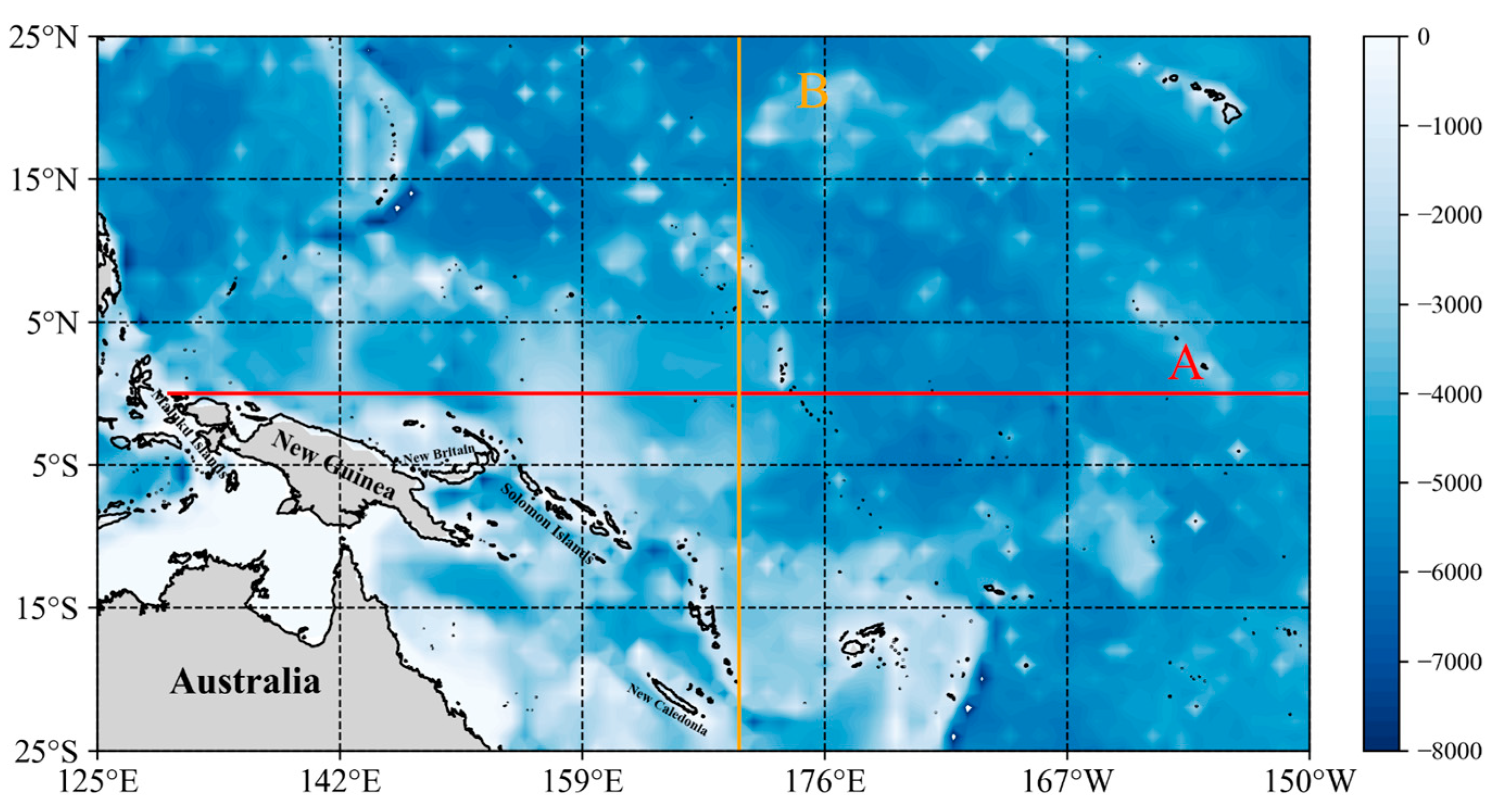
Figure 3.
Flowchart of the DO-ResNet model for estimating ocean subsurface thermohaline structure in the tropical Western Pacific.
Figure 3.
Flowchart of the DO-ResNet model for estimating ocean subsurface thermohaline structure in the tropical Western Pacific.
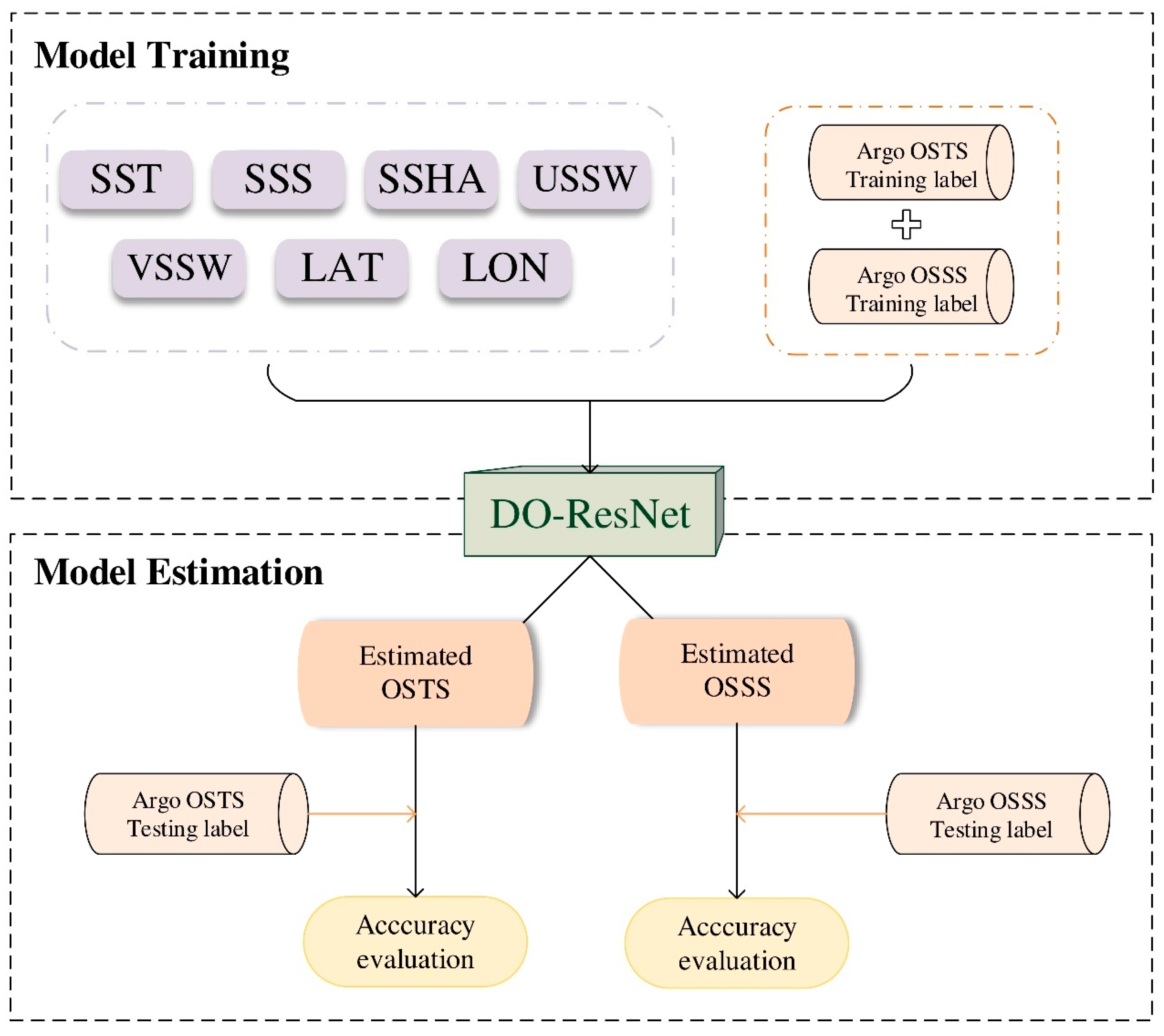
Figure 4.
The estimation accuracy of the OST (a, b) and OSS (c, d) at different depths by the DO-ResNet model based on RMSE and R2 in different cases (Cases 1, 2, 3 shown in red, blue and black lines respectively) in 2020.
Figure 4.
The estimation accuracy of the OST (a, b) and OSS (c, d) at different depths by the DO-ResNet model based on RMSE and R2 in different cases (Cases 1, 2, 3 shown in red, blue and black lines respectively) in 2020.
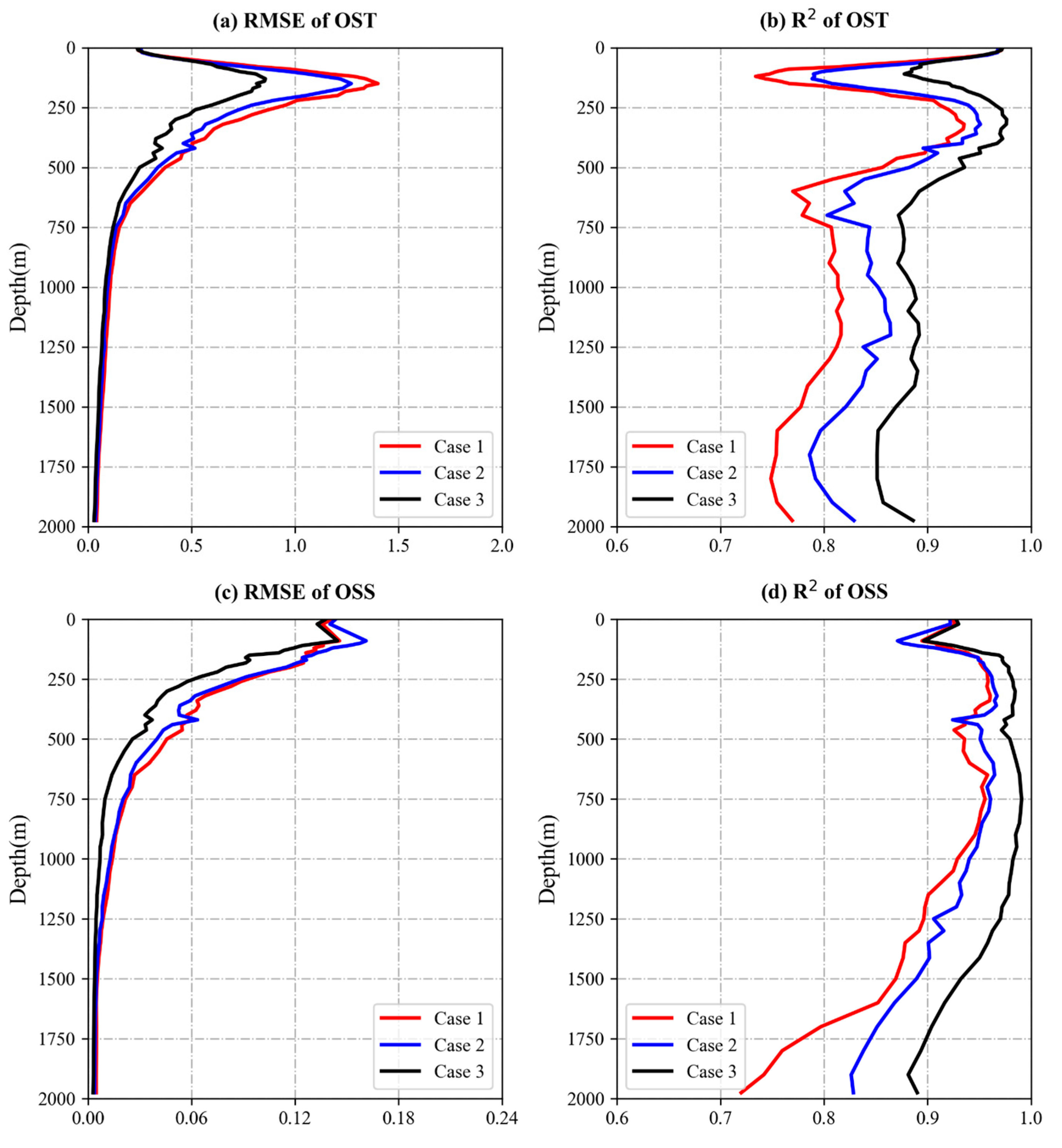
Figure 5.
Comparison of the DO-ResNet model (black lines) with three machine learning models (XGBoost: red lines, RF: blue lines, ANN: magenta lines) for OST and OSS estimation at different depths based on RMSE (a, c) and R2 (b, d) in 2019.
Figure 5.
Comparison of the DO-ResNet model (black lines) with three machine learning models (XGBoost: red lines, RF: blue lines, ANN: magenta lines) for OST and OSS estimation at different depths based on RMSE (a, c) and R2 (b, d) in 2019.

Figure 6.
Argo-derived (a, d), DO-ResNet model estimated (b, e), and their differences (Argo observations minus DO-ResNet estimates; c, f) of OST (unit:
Figure 6.
Argo-derived (a, d), DO-ResNet model estimated (b, e), and their differences (Argo observations minus DO-ResNet estimates; c, f) of OST (unit:
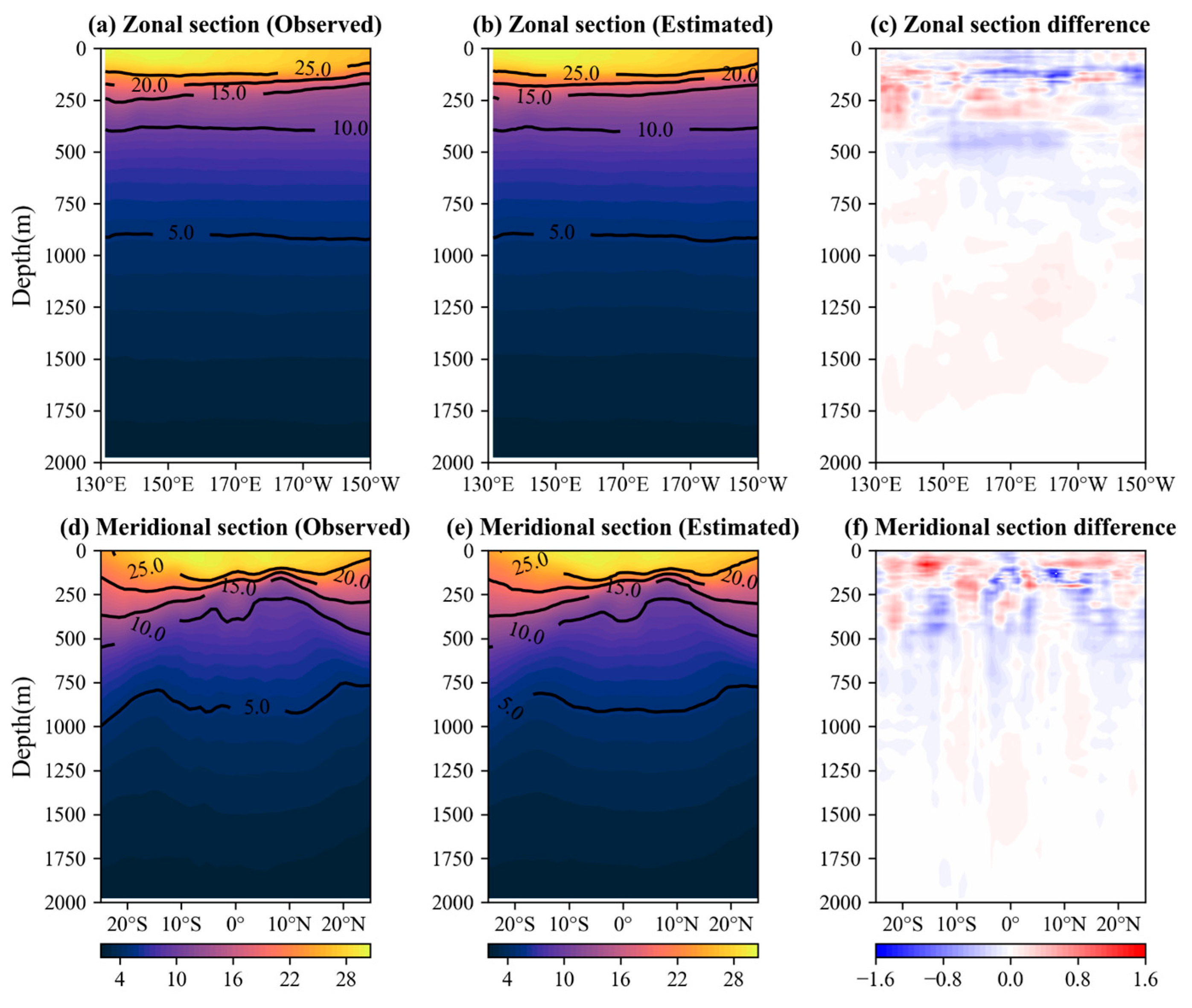
Figure 7.
Same as Figure 6 but for OSS (unit: psu).
Figure 7.
Same as Figure 6 but for OSS (unit: psu).
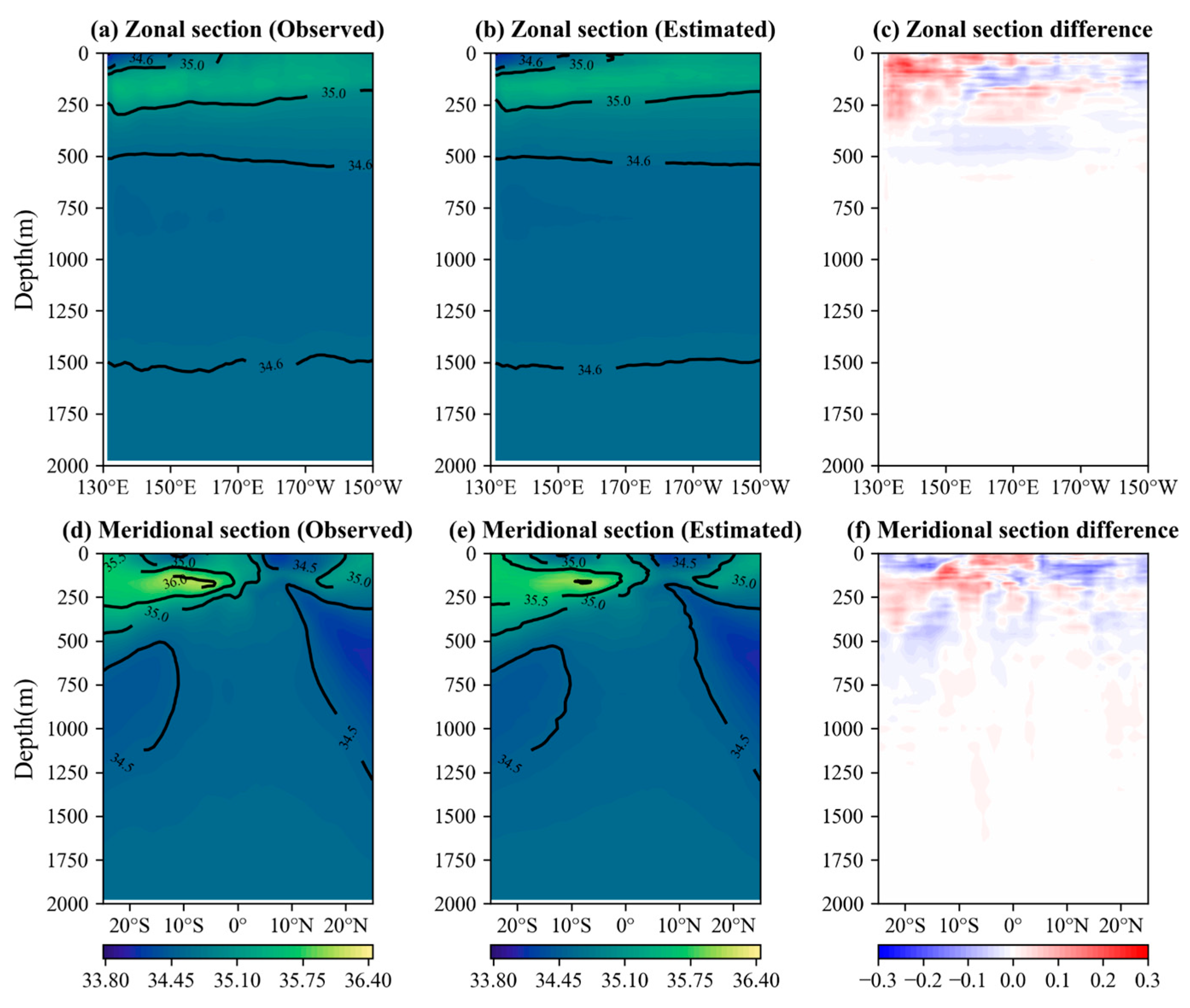
Figure 8.
Annual averaged OST (unit:
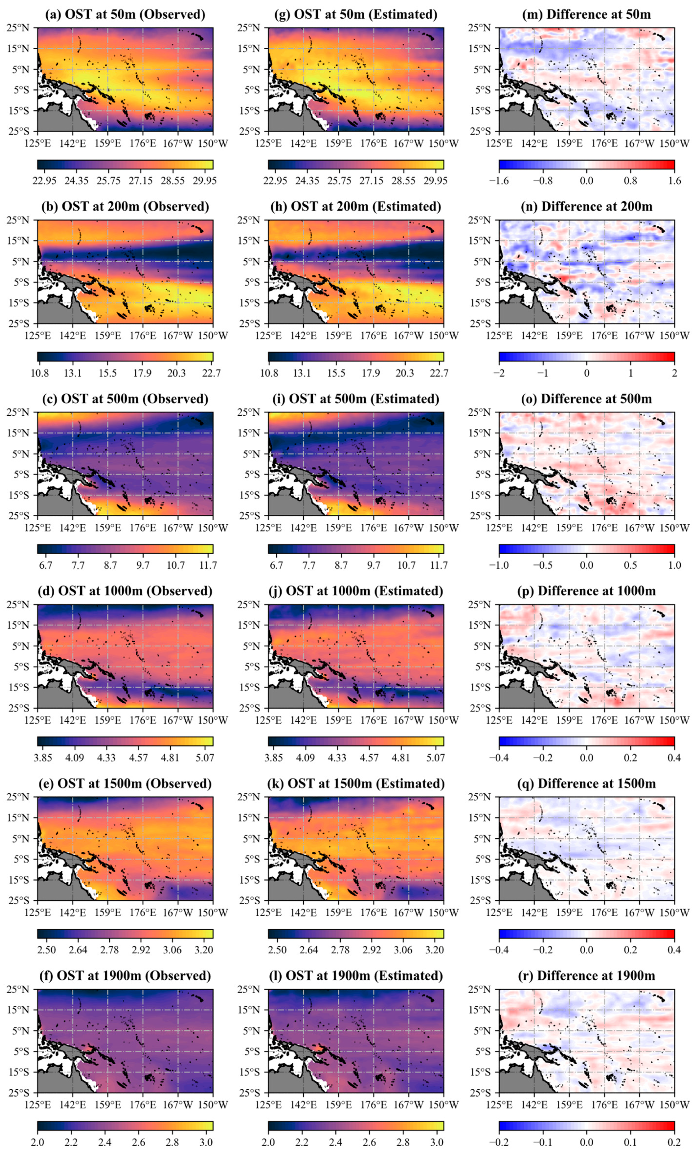
Figure 9.
Same as Figure 8 but for OSS (unit: psu).
Figure 9.
Same as Figure 8 but for OSS (unit: psu).
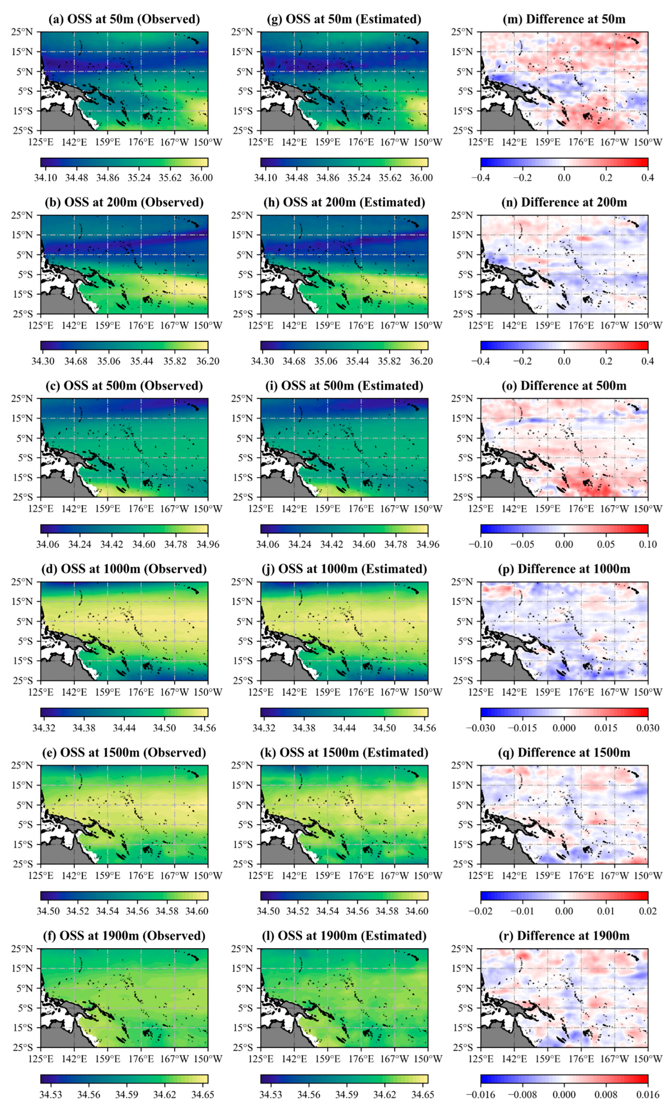
Figure 10.
Seasonal performance of the DO-ResNet model for OST (a) and OSS (b) estimation at different depths in the tropical Western Pacific in 2020. Blue indicates February (winter), orange indicates May (spring), green indicates August (summer), and red indicates November (autumn). The histograms display the NRMSE, while the lines display R2.

Figure 11.
Pearson correlation coefficients between the DO-ResNet model estimated OST (a) and OSS (b) at different depths and the observational sea surface parameters.
Figure 11.
Pearson correlation coefficients between the DO-ResNet model estimated OST (a) and OSS (b) at different depths and the observational sea surface parameters.
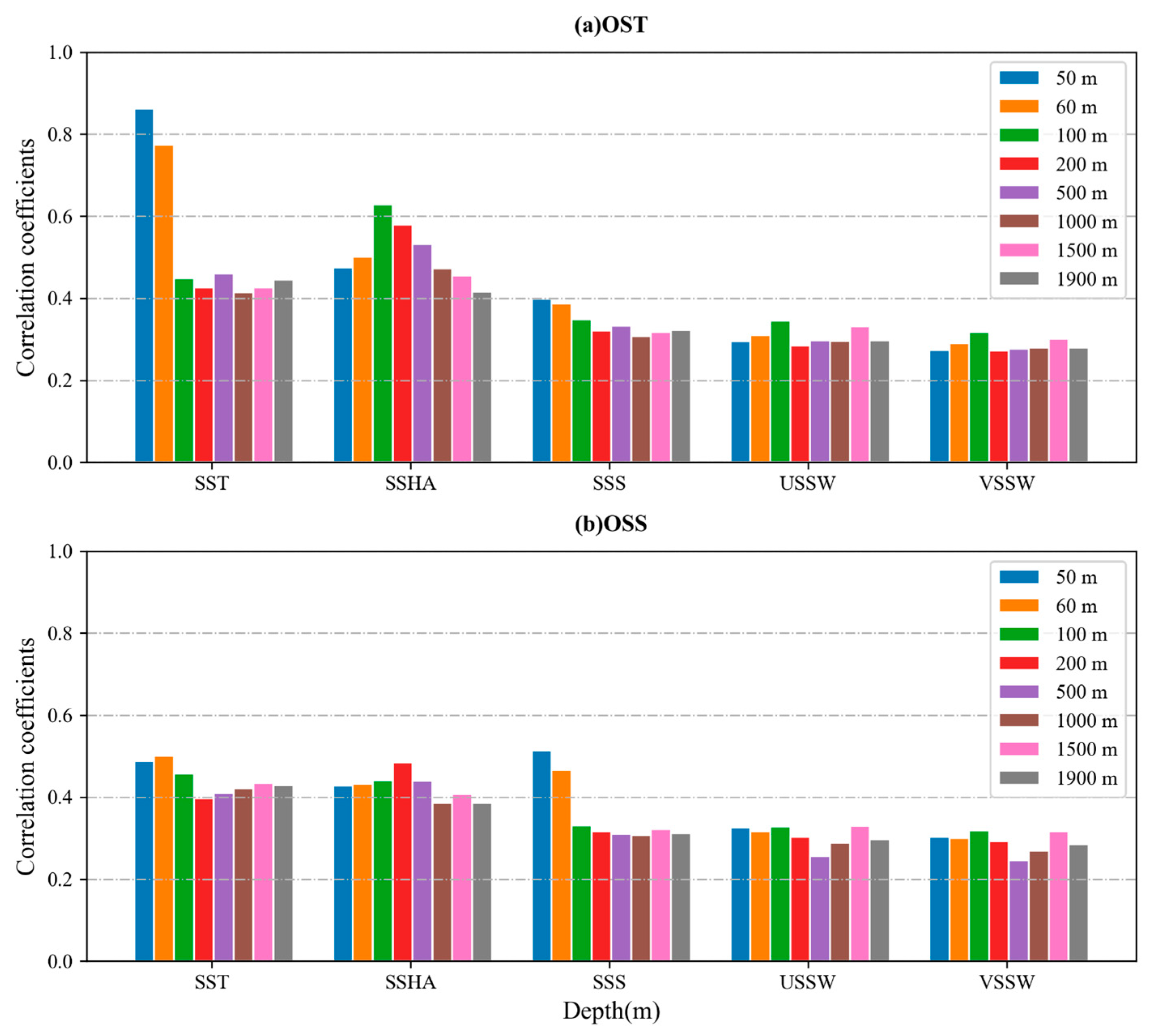

Table 1.
Summary of data used in this study.
| Index | Contents | |||
|---|---|---|---|---|
| Study Area | ) | |||
| Data | SSS | 2010-2020 | SMOS | Input |
| SST | 2010-2020 | NOAA | ||
| SSHA | 2010-2020 | AVISO | ||
| SSW | 2010-2020 | CCMP | ||
| OST | 2010-2020 | RG-Argo | Label | |
| OSS | 2010-2020 | RG-Argo | ||
| Resolution | monthly | |||
Table 2.
Parameter values of DO-ResNet models.
| Estimation Models | Parameter Values |
|---|---|
| DO-ResNet | convolutional layer: size = 3×3, stride = 1; adaptiveavgpool2d: output_size = 1×1; loss function: mse; optimizer: radam; learning rate: 0.02; reducelronplateau: mode = ‘min’, factor = 0.1, patience = 10; batch size: 2048; activation function: relu; batchnorm2d; validation frequency: per epoch earlystopping: patience = 7, verbose=False, delta=0 |
Table 3.
Presents the optimized combinations of model parameters.
| Experiments | Training Methods |
|---|---|
| Case 1 (3 parameters) | OST (OSS) = Ensemble (SST, SSS, SSHA) |
| Case 2 (5 parameters) | OST (OSS) = Ensemble (SST, SSS, SSHA, USSW, VSSW) |
| Case 3 (7 parameters) | OST (OSS) = Ensemble (SST, SSS, SSHA, USSW, VSSW, LON, LAT) |
Table 4.
Parameter values of different estimation models.
| Models | Parameter Values |
|---|---|
| XGBoost | eta = 0.02, min_child_weight = 2.0, max_depth = 5, subsample = 0.8 |
| RF | min_samples_split = 100, min_samples_leaf = 20, max_depth = 8, random_state = 10 |
| ANN | number of neural network layers = 3, learning rate = 0.002, number of neurons per layer = 30, loss function = MSE |
Disclaimer/Publisher’s Note: The statements, opinions and data contained in all publications are solely those of the individual author(s) and contributor(s) and not of MDPI and/or the editor(s). MDPI and/or the editor(s) disclaim responsibility for any injury to people or property resulting from any ideas, methods, instructions or products referred to in the content. |
© 2024 by the authors. Licensee MDPI, Basel, Switzerland. This article is an open access article distributed under the terms and conditions of the Creative Commons Attribution (CC BY) license (http://creativecommons.org/licenses/by/4.0/).
Copyright: This open access article is published under a Creative Commons CC BY 4.0 license, which permit the free download, distribution, and reuse, provided that the author and preprint are cited in any reuse.


