
Submitted:
28 March 2025
Posted:
01 April 2025
You are already at the latest version
Abstract
Total Precipitable Water (TPW) is a key variable of atmospheres, and its spatiotemporal distribution is of great importance in global climate change. This paper addresses the TPW retrieval over both sea and land surfaces from the data acquired by the Microwave Humidity Sounder II (MWHS-II) on Fengyun 3D (FY-3D) satellite. First, Back Propagation neural network (BPNN) algorithms are developed with the spatiotemporal matching samples of the MWHS-II data versus the fifth-generation European Centre for Medium-Range Weather Forecast (ECMWF) atmospheric reanalysis (ERA5) data. Then, the TPWs between 65°S and 65°N over both sea and land surfaces are retrieved from FY-3D MWHS-II data in 2022. Finally, the TPWs retrieved in this work are validated with the radiosonde TPWs over both sea and land surfaces, and they are also compared to the F18 Special Sensor Microwave Imager Sounder (SSMIS) TPWs over sea surfaces. The results indicate that the BPNN algorithms developed in this work are valid and accurate. The mean error (ME), the root mean square error (RMSE) and mean absolute error (MAE) of the TPWs retrieved in this work against the radiosonde TPWs are -1.17 mm, 3.46 mm and 2.63 mm over sea surfaces, respectively, and they are -0.80 mm, 4.04 mm and 3.13 mm over land surfaces, respectively. The TPWs retrieved in this work are much more accurate than the F18 SMMIS TPWs.
Keywords:
FY-3D MWHS-II data
; total precipitable water
; back propagation neural network
; retrieval algorithm development
; validation
1. Introduction
Total Precipitable Water (TPW) is a key physical parameter in the study of global energy balance and water cycle. Its spatiotemporal distribution and variations significantly affect global climate change, making it highly valuable for weather and climate applications [1]. Currently, TPW products are mainly obtained through three methods: the radiosonde observations, the satellite remote sensing, and the reanalysis data. The radiosonde observations provide accurate TPW by measuring humidity profiles and integrating water vapor content of the entire atmospheric column. However, the radiosonde observations are expensive and have uneven spatial distribution, especially in oceanic regions where stations are sparse. Additionally, radiosondes typically conduct measurements only twice a day, limiting their ability to monitor rapidly changing weather processes [2]. Another method to obtain TPW is through satellite remote sensing, which can be divided into optical, infrared, and microwave remote sensing. The optical remote sensing has a high spatial resolution, but it is greatly affected by clouds. The infrared remote sensing also cannot effectively retrieve water vapor information under cloudy conditions. In contrast, the microwave remote sensing can penetrate cloud layers and acquire data in cloudy conditions, enabling all-weather TPW observation [3]. However, the accuracy of microwave remote sensing retrieval is strongly influenced by the surface emissivity, which usually has large value and uncertainty over land, which makes it difficult to distinguish atmospheric signals from surface radiation. Fortunately, the microwave sea surface emissivity has smaller value and less variation in contrast to microwave land surface emissivity. Therefore, the TPW retrieval over sea surfaces is far more accurate than that over land surfaces. So far, most existing studies focus on the TPW retrieval over sea surfaces [4].
The research on TPW retrieval from satellite microwave radiometer data has a history of several decades, and many methods have been developed, including the empirical methods, the semi-empirical methods, the physics-based methods, and the neural network methods [5,6,7]. These methods generally perform retrieval by establishing linear or nonlinear relationships between TPW and the brightness temperatures (TB) in microwave channels. Currently, microwave radiometers primarily use two water vapor absorption lines, located at 22.235 GHz and 183.31 GHz, to detect atmospheric moisture information. Grody et al. first validated the strong correlation between water vapor content and TB at the 22.235 GHz water vapor absorption line and proposed an empirical method to retrieve atmospheric water vapor content from microwave radiometer observations [8]. Alishouse et al. utilized the Special Sensor Microwave Imager (SSM/I) observations to simultaneously retrieve the TPW and cloud liquid water content over sea surfaces [9]. According to a radiative transfer model, Wang et al. developed a semi-empirical algorithm to retrieve the total water vapor content over sea surfaces from the Tropical Rainfall Measuring Mission (TRMM) Microwave Imager (TMI) data under clear-sky conditions [10]. Bobylev et al. developed a neural network algorithm to retrieve water vapor content over the Arctic Ocean [11] from the combined SSM/I data and the data acquired by the Advanced Microwave Scanning Radiometer for the Earth Observing System (AMSR-E). In contrast to the 22.23 GHz channel, the channels centered at the 183.31 GHz water vapor absorption line offer higher spatial resolution and observation accuracy, and have been widely used to retrieve TPW in recent years. The modern advanced satellite microwave radiometers, such as the Advanced Microwave Sounding Unit B (AMSU-B), the Microwave Humidity Sounder (MHS), and the Advanced Technology Microwave Sounder (ATMS), are equipped with the 183.31 GHz channels. Boukabara et al. proposed a variational retrieval algorithm and established a comprehensive microwave retrieval system (MiRS). With the data in the 183.31 GHz channels, the TPW retrieval accuracy was significantly improved [12]. Liu et al. developed a physics-based algorithm to retrieve TPW from the ATMS observations in the 165.50 GHz and 183.31 GHz channels [13].
The Fengyun-3 (FY-3) series are China’s second generation of polar-orbiting meteorological satellites. The fourth satellite in the series, FY-3D, was successfully launched from the Taiyuan Satellite Launch Center on November 15, 2017. It is China’s main operational low Earth orbit afternoon satellite. There are ten advanced remote sensing instruments on FY-3D, and one of them is the Microwave Humidity Sounder II (MWHS-II) [14]. As listed in Table 1, the MWHS-II has four frequency bands and fifteen channels. Among these, the 118.75 GHz oxygen-absorption band is used for the first time on a polar-orbiting meteorological satellite. This band has eight oxygen absorption channels at the Quasi-vertical (QV) polarization, which are mainly used to detect atmospheric temperature profiles. The 183.31 GHz water vapor absorption band has five channels at the QV polarization, which are primarily used to retrieve atmospheric humidity profiles. In addition, two window channels are centered at 89.0 GHz and 150.0 GHz at the Quasi-horizontal (QH) polarization, respectively, and they are used to collect radiation and scattering from both the Earth surfaces and atmospheres. The equivalent noise temperature difference (NEΔT) is 1.0 K in the channels 1 and 8~15, 1.6 K in the channels 4~7, 2.0 K in the channel 3, and 3.6 K in the channel 2 [15]. FY-3D MWHS-II cross-track scans Earth surfaces and atmospheres with the 15 channels, and the Earth Incidence Angle (EIA) mainly ranges between 0° and 65°. According to the instrument parameters, the FY-3D MWHS-II’s observations can be used to retrieve global TPW.
2. Study Data and Processing
In this work, the following data in 2022 are used: the FY-3D MWHS-II Level 1 (L1) data, the fifth-generation of European Centre for Medium-range Weather Forecast (ECMWF) atmospheric reanalysis (ERA5) data, the radiosonde data, the F18 Special Sensor Microwave Imager Sounder (SSMIS) TPW product, the Terra and Aqua combined Moderate Resolution Imaging Spectroradiometer (MODIS) land cover (MCD12C1) product, and the Global 30 Arc-Second Elevation (GTOPO30) data.
The FY-3D MWHS-II L1 data, provided by the Fengyun Satellite Data Center (https://satellite.nsmc.org.cn), contain the TBs at top of atmosphere (TOA) in the fifteen channels listed in Table 1, the geolocation (longitude and latitude), the observation time, the EIA, etc.
The ERA5 data (https://cds.climate.copernicus.eu) contain hourly estimates of a lot of atmospheric, land and oceanic climate variables with longitude and latitude resolutions of 0.25˚×0.25˚ [16]. In this work, only the single-layer ERA5 Total Column Water (TCW) data are used to build the sample datasets below.
The radiosonde data, provided by the University of Wyoming in the United States of America (USA) (http://weather.uwyo.edu/upperair/sounding.html), have climate parameters at 0:00 and 12:00 UTC every day, such as the profiles of atmospheric temperature and humidity, wind speed and direction, etc. In this work, the TPWs extracted from the radiosonde atmospheric humidity profiles are used to validate the results in this work. The extraction equation is given below [17]:
where ρ is the air density, g is the gravitational acceleration, q(p) denotes the specific humidity at pressure p, and ps is the pressure at Earth surface.
The F18 SSMIS TPW product (http://www.remss.com) is generated from the observations acquired by the SSMIS on the U.S. Defense Meteorological Satellite Program (DMSP) F18 satellite in terms of the radiative transfer model [18], and it provides TPWs over sea surfaces with a spatial resolution of 0.25° in both longitude and latitude. The validation results indicated that the F18 SSMIS TPW has a good accuracy. Therefore, The F18 SSMIS TPWs are used to cross-validate the results over sea surfaces in this work.
The MCD12C1 product (https://search.earthdata.nasa.gov), generated from the observations of the MODIS [19], provides global land cover types with a spatial resolution of 0.05° (approximately 5.6 km) in both longitude and latitude. According to the standards of International Geosphere-Biosphere Programme (IGBP), the MCD12C1 product divides global land surfaces into 17 major categories, including 11 natural vegetation types, three human-developed and land mosaic types, and three non-vegetated land types. The land cover types extracted from the MCD12C1 product are used as one of the input features over land surfaces.
The GTOPO30 dataset (https://www.usgs.gov) is a global digital elevation model (DEM) produced by the U.S. Geological Survey (USGS). It covers global land areas with a spatial resolution of 30 arc-seconds (approximately 1 km) [20]. The GTOPO30 dataset provides elevation information for the entire globe and is widely used in geographic and climate change research, hydrological analysis, and ecological modeling. In this work, the GTOPO30 elevation data are used to determine the Earth surface-atmosphere boundary and used as one of the input features over land surfaces.
Except the ERA5 data and the F18 SSMIS TPW data, all the data introduced above are firstly pixel-aggregated into the 0.25°×0.25° grid space. Then, the TBs in the MWHS-II channels 10 to 15 are re-calibrated using the intercalibration results in [21]. Finally, two datasets mainly containing the spatiotemporal sample data between FY-3D MWHS-II TBs and the ERA5 TPW in 2022 are collected for sea surfaces and land surfaces, respectively. The matching criteria are 1) collocation in the 0.25 °×0.25 ° grid space between 65 °S and 65 °N at least 25 km far away from coastlines, and 2) a maximum absolute time difference of one minute. According to the above criteria, a total of 14,107,205 matching samples over sea surfaces and 6,300,924 matching samples over land surfaces are collected. Figure 1 displays the spatial distribution of the matching samples over both sea surfaces and land surfaces. The matching samples are densely distributed in high latitude regions, followed by the tropical regions and the mid-latitude regions. In most regions, the number of matching samples is greater than fifteen. Table 2 lists the monthly distribution of the matching samples. Over land surfaces, the number of matching samples ranges between 465,000 and 549,000, whereas it is approximately doubled over sea surfaces. The spatiotemporal distribution of the matching samples is determined by many factors, such as the satellite orbit, the matching criteria, and so on. In general, the matching samples have good spatiotemporal representativeness, and can be used to develop the TPW retrieval algorithm.
It should be noted that, the features in the two datasets have different units, e.g., the TBs are in K, while the elevation is in kilometer. To eliminate the impact of different units of input features on the output and accelerate the convergence of the neural network training, all the input data in the two datasets are converted into the z-scores using the following equation
where μ and σ are the mean and the standard deviation of input feature x, respectively; zi is the z-score of input xi.
3. Methodology
3.1. Back Propagation Neural Network (BPNN)
To retrieve TPW over both sea surfaces and land surfaces, the Back Propagation Neural Network (BPNN) [22] is adopted in this work. As shown in Figure 1, the BPNN consists of the input layer, the hidden layer(s), and the output layer.
Figure 2.
Architecture of the Back Propagation Neural Network (BPNN) for TPW Retrieval.
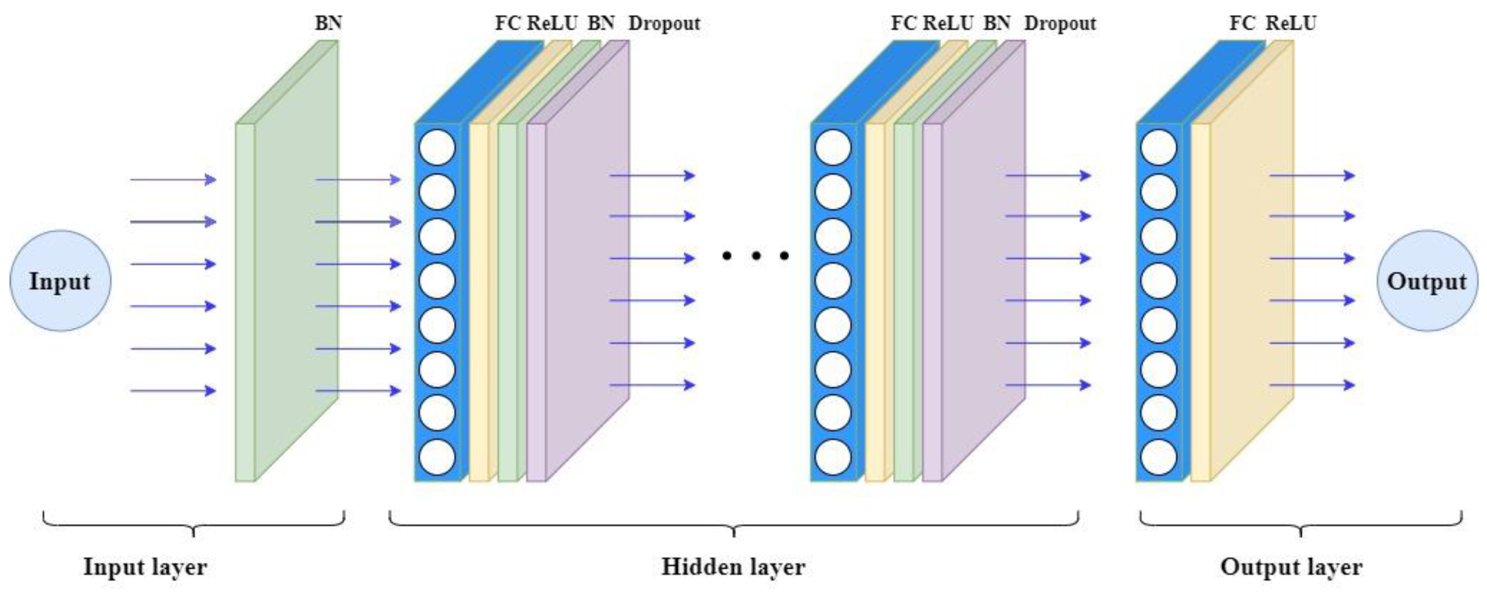
Because of the large differences between land surfaces and sea surfaces, two BPNNs are designed for the TPW retrieval over sea and land surfaces, respectively. As we know, the hyperparameter selection is essential for optimizing the performance of neural networks. In this work, with randomly selected 80% of the matching samples as training data and the remaining 20% as the testing data, ablation experiments are conducted with the following candidate settings: the number of hidden layer(s) of 1, 2, 3 or 4, the number of neurons per hidden layer of 32, 64, 128 or 256, the loss function of Mean Square Error (MSE) Loss, Mean Absolute Error (MAE) Loss, Huber Loss or Log-Cosh Loss, and the dropout rate of 0.0, 0.1, 0.2, 0.3 or 0.5. The results of ablation experiments indicate that for sea surfaces, the BPNN with a single hidden layer of 128 neurons, the MSE Loss function, and the dropout rate of 0.1 provides the best balance between predicting accuracy and computational efficiency. For land surfaces, the BPNN with two-hidden-layer of 64 neurons per layer, the MSE Loss function, and the dropout rate of 0.2 shows superior performance. These optimized settings ensure the robustness and generalization of the BPNN models across diverse atmospheres and Earth surfaces, highlighting the importance of tailoring hyperparameters to the specific retrieval task.
Because the atmospheric humidity is coupled with the atmospheric temperature, besides the TBs in the water vapor absorption channels, the use of TBs in the oxygen-absorption channels can improve the humidity retrieval accuracy [23]. In addition, the TBs in the MWHS-II channels 1 (89.0 GHz) and 10 (150.0 GHz) can provide information from Earth surfaces. Therefore, the TBs in all the fifteen MWHS-II channels are used in TPW retrieval in this work. Over sea surfaces, 19 input features are used, and they are the 15 TBs extracted from the FY-3D MWHS-II L1 data, the month of the year, the geolocation (latitude and longitude), and the EIA. Because of relatively small values and narrow dynamic ranges, the sea surface emissivities in the MWHS-II channels 1 (89.0 GHz) and 10 (150.0GHz) are not taken into account. While over land surfaces, due to the complexity of land surfaces, besides the 19 input features for sea surfaces, other six variables are selected as input features: the GTOPO30 elevation, the MCD12C1 land cover type, and four land surface emissivities in the MWHS-II channels 1 (89.0 GHz) and 10 (150.0 GHz) at both vertical and horizontal polarizations. In this work, the land surface emissivities are calculated using the Hewison’s model [24]. In addition, the ablation experiments also show that the use of squares of the TBs instead of the TBs themselves can improve the model’s sensitivity to the TB’s nonlinear variations, and the use of exponential value of the elevation instead of the elevation itself can reduce the scaling effect of elevation data on the model and enhance the model’s generalization capability and stability.
The hidden layer is composed of a fully connected (FC) layers, a Rectified Linear Unit (ReLU) activation function, a batch normalization (BN) layer, and a dropout. The ReLU activation function accelerates convergence and mitigates the gradient vanishing problem; the BN layer stabilizes the training process, and the dropout reduces the risk of overfitting and gradient explosion [25].
The output layer consists of one neuron, which corresponds to the TPW and is fully connected to the neurons in the previous layer, and the ReLU activation function and the MSE loss function are applied.
Once the structures and settings are determined, the BPNNs are trained using the error back-propagation method fed with the training data and testing data.
Figure 3 displays the testing results of the trained BPNNs with testing data over sea surfaces and land surfaces. The scatters are distributed around the diagonals, and the predicted TPWs are linearly related to the ERA5 TPWs. Over sea surfaces, the mean error (ME), the root mean square error (RMSE), the mean absolute error (MAE) and the determinant coefficient (R2) are 0.04 mm, 2.04 mm, 1.47 mm and 0.98, respectively. Over land surfaces, the scatters are relatively more dispersed in contrast to those over sea surfaces, and the ME, the RMSE, MAE and R2 are 0.06 mm, 2.60 mm, 1.75 mm and 0.97, respectively. The results indicate that the predicting errors over land surfaces are slightly greater than those over sea surfaces. This is mainly attributed to the complex of land surfaces, especially the uncertainties of land surface emissivities, which are estimated by the Hewison’s model and more accurate over vegetated areas than over bare areas [24,26].
Land cover types have impact on TPW retrieval [27]. Figure 4 shows the testing results across the 17 MODIS land cover types. The predicted TPWs are highly linear related to the ERA5 TPWs with R2 greater than or equal to 0.92, except that over the snow and ice areas, which is 0.86. The ME ranges between -0.56 mm and 0.35 mm. The RMSE (MAE) varies from 1.47 (1.03) mm to 3.49 (2.47) mm depending on land cover types. Overall, the RMSEs (MAEs) over the three non-vegetated or sparsely vegetated areas (the water bodies, snow and ice, and barren or sparsely vegetated areas) are smallest, the RMSEs (MAEs) over the 11 natural vegetation areas are in the middle, and the RMSEs (MAEs) over the three human-developed and mosaic areas (the croplands, urban and built-up, and cropland/natural vegetation mosaic areas) are largest. These differences mainly come from the land cover types and the complex interaction between land and atmosphere. In general, the testing results in this work basically agree with those in [27,28]. The results demonstrate that the BPNN model in this work is not only applicable to all land cover types, but also has excellent performance.
To further evaluate the contributions and importance of input features in TPW retrieval, the SHapley Additive exPlanations (SHAP) method is used. The SHAP is a model interpretation technique rooted in cooperative game theory, and it quantifies feature importance by calculating the marginal contribution of each feature to the model’s output [29]. Figure 5 demonstrates the SHAP analysis results of the BPNNs over both sea surfaces and land surfaces. Over sea surfaces, the five most important features are the TB9, TB1, EIA, TB13, and TB10, respectively, while the five least important features are TB4, the longitude, TB3, TB2 and the month, respectively, where the TBi denotes the TB in MWHS-II channel i. Over land surfaces, the five most important features are TB15, TB13, TB8, TB9 and TB6, respectively, whereas the five least important features are the land cover types, TB3, longitude, TB2 and the month, respectively. The land surface emissivities in the channels 1 (89.0 GHz) and 10 (150.0 GHz) and the elevation also make significant contributions on the TPW retrieval over land surfaces. Over both sea and land surfaces, the TBs in the MWHS-II oxygen-absorption channels centered at 118.75 GHz have obvious contributions on TPW retrieval. The SHAP results justify that the selection of the input features is reasonable.
In general, the BPNNs are well designed, and both the training and testing results indicate that the BPNNs have good accuracy, strong robustness and generalization capability in TPW retrieval.
3.2. Comparison to Other Commonly Used Methods
To further evaluate the retrieval performance, the BPNNs developed in this work are compared to seven commonly used methods with the same training data and testing data in Section 2. The seven methods are the D-matrix method [30], the Ridge method [31], the Lasso method [32], the physical method [33], the random forest (RF) method [34], the support vector machine (SVM) method [35], and the eXtreme Gradient Boosting (XGBoost) method [36]. The first three methods are statistical ones, while the last three methods are the machine learning ones. The physical method is not applied to the TPW retrieval over land surfaces because of its poor performance over land surfaces [33]. The following six standard statistical metrics are used for quantitative analysis: the ME, the MAE, the RMSE, the mean squared logarithmic error (MSLE), the mean absolute percentage error (MAPE), and R2. Besides the testing results of the seven methods, the testing results of the BPNNs are listed in Table 3 for convenience. Over sea surfaces, the ME, MAE, RMSE, MAPE, MSLE and R2 of the BPNN in this work are 0.04 mm, 1.47 mm, 2.04 mm, 0.01 mm, 8.64% and 0.982, respectively. Except the ME, the BPNN in this work is far superior to the seven methods on other statistical metrics. Over land surfaces, the ME, MAE, RMSE, MSLE, MAPE and R2 of the BPNN in this work are, respectively, 0.06 mm, 1.79 mm, 2.60 mm, 0.03 mm, 15.53% and 0.967, which are slightly worse than those of the BPNN over sea surfaces. However, the BPNN over land surfaces is superior to other six methods on all metrics. It should be noted that, the XGBoost method achieved good results second only to the BPNNs in this work. In general, the BPNNs in this work have good performance in TPW retrieval over both sea and land surfaces.
4. Results and Analysis
The global TPWs are retrieved from the FY-3D MWHS-II data in 2022 using the BPNNs developed in Section 3.
Taking the results on January 1, April 1, July 1 and October 1 of 2022 as examples, Figure 6 displays the maps of TPWs retrieved from the MWHS-II data over both sea and land surfaces. The TPW mainly ranges between 0.0 and 75.0 mm, and obviously depends on latitude: the TPW usually has large value in the tropical region, and gradually decreases towards high latitude. The relatively large TPW in the tropical region is mainly attributed to the strong evaporation and deep convection, especially in the Pacific Ocean, the Indian Ocean, the Atlantic Ocean, the Amazon tropical rain forests, the West Africa rain forests, and the Southeast Asian archipelago.
Over the sea surfaces in the mid-latitude regions, because of subtropical high-pressure systems and mid-latitude cyclonic activities, several distinct moisture transport belts are observed. They move towards south in January, and move toward north in July. In contrast to sea surfaces, the TPW distribution over land surfaces is more complicated, varying with season and location. The regions with large TPW are mainly distributed in the Central African Basin, the Southeast Asian archipelago (including Indonesia), and the tropical rainforest regions of Central and South America. These regions are significantly influenced by tropical monsoons, strong convection, and abundant precipitation. The TPW in mid-latitude regions of the Northern Hemisphere is generally lower, especially in winter, due to the dominance of dry continental air under cold high-pressure systems.
The TPWs retrieved in this work are validated with the TPWs extracted from the radiosonde data provided by the University of Wyoming in USA. The TPWs in this work are matched to the radiosonde data with the following two criteria: 1) the radiosonde stations fall in the 0.25°×0.25° grid at least 25 km away from the continent coastlines, and 2) the absolute time difference is less than 3 hours. As shown in Figure 7, 16 deep-sea radiosonde stations located on islands and 135 continent stations are qualified. The TPWs of the radiosonde data are calculated using Eq. (1). A total of 4,613 matching TPWs over sea surfaces and 71,577 matching TPWs over land surfaces are collected in 2022.
Because the deep-sea radiosonde stations are located on islands, which are higher than sea surfaces in altitude. This means that the retrieved TPWs over sea surfaces are slightly larger than the TPWs extracted from the radiosonde data. Bock et al. proposed an altitude correction term for TPW [37], which is given by
where Δω is the correction term for the TPW ω, and h is the altitude of the deep-sea radiosonde station in meters.
The TPWs at deep-sea stations are corrected by adding the ΔTPW. After the altitude correction, the retrieved TPWs are more consistent with the radiosonde TPWs. Figure 8 displays the scatter plots of the TPWs retrieved in this work versus the radiosonde TPWs. The TPWs retrieved in this work are highly linearly related to the radiosonde TPWs with determinant coefficients (R2) greater than 0.96. The scatters over sea surfaces are more concentrated around the diagonal than those over land surfaces. Over sea surfaces, the ME, the RMSE and MAE are, respectively, -1.17 mm, 3.46 mm and 2.63 mm, while over land surfaces, they are -0.80 mm, 4.04 mm and 3.13 mm, respectively. Against the radiosonde TWs, the TPWs in this work are averagely underestimated, which may be due to the discrepancy between the ERA5 data and the radiosonde data [38]. The retrieved TPWs over land surfaces have relatively larger errors than those over sea surfaces, because of the larger variations in both land surfaces and atmospheres, and the complex interaction between them. In general, the TPWs retrieved in this work are accurate against the radiosonde TPWs over both sea surfaces and land surfaces.
The TPWs retrieved in this work are also compared to the F18 SSMIS TPWs in 2022. It should be noted that, the F18 SSMIS TPW product only provides TPWs over sea surfaces, and consequently the comparison is conducted only over sea surfaces. Using the same matching criteria, 1559 matching samples between F18 SSMIS TPWs and radiosonde TPWs are collected. Figure 9 shows the scatter plot of the F18 SSMIS TPWs versus the radiosonde TPWs. Against the radiosonde TPWs, the ME, the RMSE and MAE of F18 SSMIS TPWs are, respectively, 0.86 mm, 4.24 mm and 3.37 mm. The RMSE and MAE of F18 SSMIS TPWs are 0.78 mm and 0.74 mm larger than those of the TPWs retrieved in this work, respectively. The determinant coefficient (R2) of the F18 SSMIS TPWs is 0.92, which is also less than the one of the TPWs retrieved in this work. Therefore, a conclusion can be made that the TPWs retrieved in this work are more consistent with the radiosonde TPWs than the F18 SSMIS TPWs, i.e., the TPWs retrieved in this work are more accurate than the F18 SSMIS TPWs.
5. Summary and Conclusion
This paper presented the TPW retrieval from FY-3D MWHS-II L1 data over both sea and land surfaces. First, the BPNNs were developed with the matching samples between the MWHS-II data and the ERA5 TPWs. Then, the TPWs between 65ºS and 65ºN were retrieved from the MWHS-II data in 2022. Finally, the TPWs retrieved in this work were validated with the radiosonde TPWs, and compared to F18 SSMIS TPWs. The results indicated that the BPNN algorithms developed in this work are valid and accurate, which are superior to the D-matrix method, the Ridge method, the Lasso method, the physical method, the RF method, the SVM method and the XGBoost method. The ME, the RMSE and MAE of the TPWs retrieved in this work against the radiosonde TPWs are -1.17 mm, 3.46 mm and 2.63 mm over sea surfaces, respectively, and they are -0.80 mm, 4.04 mm and 3.13 mm over land surfaces, respectively. The TPWs retrieved in this work are much more accurate than the F18 SMMIS TPWs.
The TPWs retrieved in this work were averagely underestimated against the radiosonde TPWs, which may be attributed to the discrepancy between the ERA5 data and radiosonde data. In the future, the ERA5 total column water will be fully evaluated using the radiosonde data.
Author Contributions
Conceptualization, G.J.; methodology, G.J. and Y.Z.; software, Y.Z.; validation, Y.Z., G.J. and G.W.; formal analysis, G.J.; investigation, G.J.; resources, Y.Z.; data curation, Y.Z., and G.W.; writing—original draft preparation, Y.Z.; writing—review and editing, G.J.; visualization, Y.Z.; supervision, G.J.; project administration, G.J.; funding acquisition, G.J.
Funding
This work was supported in part by the National Key Research and Development Program of China under Grant 2021YFB3900401, and in part by the National Natural Science Foundation of China under Grant 41871222.
Data Availability Statement
Data available on request due to privacy restrictions.
Acknowledgments
Thanks are given to the National Satellite Meteorological Center, Beijing, China for providing the FY-3D MWHS-II L1 data.
Conflicts of Interest
The authors declare no conflicts of interest.
References
- Zveryaev, I.I.; Allan, R.P. Water vapor variability in the tropics and its links to dynamics and precipitation. J. Geophys. Res. Atmos. 2005, 110, D21. [Google Scholar] [CrossRef]
- Ji, D.; Shi, J.; Letu, H.; Li, W.; Zhang, H.; Shang, H. A Total precipitable water product and its trend analysis in recent years based on passive microwave radiometers. IEEE J. Sel. Top. Appl. Earth Obs. Remote Sens. 2021, 14, 7324–7335. [Google Scholar] [CrossRef]
- Ji, D.; Shi, J.; Xiong, C.; Wang, T.; Zhang, Y. A total precipitable water retrieval mthod over land using the combination of passive microwave and optical remote sensing. Remote Sens. Environ. 2017, 191, 313–327. [Google Scholar] [CrossRef]
- Schröder, M.; Lockhoff, M.; Forsythe, J.M.; Cronk, H.Q.; Vonder Haar, T.H.; Bennartz, R. The GEWEX water vapor assessment: results from intercomparison, trend, and homogeneity analysis of total column water vapor. J. Appl. Meteorol. Climatol. 2016, 55, 1633–1649. [Google Scholar] [CrossRef]
- Alshawaf, F.; Fuhrmann, T.; Knöpfler, A.; Luo, X.; Mayer, M.; Hinz, S.; Heck, B. Accurate estimation of atmospheric water vapor using GNSS observations and surface meteorological data. IEEE Trans. Geosci. Remote Sens. 2015, 53, 3764–3771. [Google Scholar] [CrossRef]
- Czajkowski, K.P.; Goward, S.N.; Shirey, D.; Walz, A. Thermal remote sensing of near-surface water vapor. Remote Sens. Environ. 2002, 79, 253–265. [Google Scholar] [CrossRef]
- Firsov, K.M.; Chesnokova, T.Y.; Bobrov, E.V.; Klitochenko, I.I. Total water vapor content retrieval from sun photometer data. Atmos. Ocean. Opt. 2013, 26, 281–284. [Google Scholar] [CrossRef]
- Grody, N.C.; Gruber, A.; Shen, W.C. Atmospheric water content over the tropical pacific derived from the nimbus-6 scanning microwave spectrometer. J. Appl. Meteorol. Climatol. 1980, 19, 986–996. [Google Scholar] [CrossRef]
- Alishouse, J.C.; Snyder, S.A.; Vongsathorn, J.; Ferraro, R.R. Determination of oceanic total precipitable water from the SSM/I. IEEE Trans. Geosci. Remote Sens. 1990, 28, 811–816. [Google Scholar] [CrossRef]
- Wang, Y.; Shi, J.; Wang, H.; Feng, W.; Wang, Y. Physical statistical algorithm for precipitable water vapor inversion on land surface based on multi-source remotely sensed data. Sci. China Earth Sci. 2015, 58, 2340–2352. [Google Scholar] [CrossRef]
- Bobylev, L.P.; Zabolotskikh, E.V.; Mitnik, L.M.; Mitnik, M.L. Atmospheric water vapor and cloud liquid water retrieval over the arctic ocean using satellite passive microwave sensing. IEEE Trans. Geosci. Remote Sens. 2009, 48, 283–294. [Google Scholar] [CrossRef]
- Boukabara, S.A.; Garrett, K.; Chen, W.; Iturbide-Sanchez, F.; Grassotti, C.; Kongoli, C.; Meng, H. MiRS: An all-weather 1DVAR satellite data assimilation and retrieval system. IEEE Trans. Geosci. Remote Sens. 2011, 49, 3249–3272. [Google Scholar] [CrossRef]
- Liu, H.; Tang, S.; Hu, J.; Zhang, S.; Deng, X. An improved physical split-window algorithm for precipitable water vapor retrieval exploiting the water vapor channel observations. Remote Sens. Environ. 2017, 194, 366–378. [Google Scholar] [CrossRef]
- Zhang, P.; Lu, Q.; Hu, X.; Gu, S.; Yang, L.; Min, M.; Xian, D. Latest progress of the chinese meteorological satellite program and core data processing technologies. Adv. Atmos. Sci. 2019, 36, 1027–1045. [Google Scholar] [CrossRef]
- Carminati, F.; Atkinson, N.; Candy, B.; Lu, Q. Insights into the microwave instruments onboard the fengyun-3d satellite: data quality and assimilation in the met office NWP System. Adv. Atmos. Sci. 2021, 38, 1379–1396. [Google Scholar] [CrossRef]
- Hersbach, H.; Bell, B.; Berrisford, P.; Hirahara, S.; Horányi, A.; Muñoz-Sabater, J.; Thépaut, J.-N. The ERA5 global reanalysis. Q. J. R. Meteorol. Soc. 2020, 146, 1999–2049. [Google Scholar] [CrossRef]
- Gurbuz, G.; Jin, S. Long-term variations of precipitable water vapor estimated from GPS, MODIS and radiosonde observations in Turkey. Int. J. Climatol. 2017, 37, 5170–5180. [Google Scholar] [CrossRef]
- Kroodsma, R.A.; Berg, W.; Wilheit, T.T. Special sensor microwave imager/sounder updates for the global precipitation measurement V07 data suite. IEEE Trans. Geosci. Remote Sens. 2022, 60, 1–11. [Google Scholar] [CrossRef]
- Sulla-Menashe, D.; Gray, J.M.; Abercrombie, S.P.; Friedl, M.A. Hierarchical mapping of annual global land cover 2001 to present: the MODIS collection 6 land cover product. Remote Sens. Environ. 2019, 222, 183–194. [Google Scholar] [CrossRef]
- Miliaresis, G.C.; Argialas, D.P. Segmentation of physiographic features from the global digital elevation model/GTOPO30. Comput. Geosci. 1999, 25, 715–728. [Google Scholar] [CrossRef]
- Zhang, Y.; Jiang, G. Intercalibration of FY-3D MWHS-II water vapor absorption channels against S-NPP ATMS channels using the double difference method. Proc. IEEE IGARSS 2024, 6255–6258. [Google Scholar]
- Yu, W.; Xu, X.; Jin, S.; Ma, Y.; Liu, B.; Gong, W. BP neural network retrieval for remote sensing atmospheric profile of ground-based microwave radiometer. IEEE Geosci. Remote Sens. Lett. 2021, 19, 1–5. [Google Scholar] [CrossRef]
- Meng, S.; Zhang, T.; Jiang, G.; Ye, H. Retrieval of atmospheric temperature and humidity profiles from FY-3E MWTS and MWHS data using deep learning neural networks. Proc. SPIE ICGRSM 2024, 12980, 564–569. [Google Scholar]
- Hewison, T.J. Airborne measurements of forest and agricultural land surface emissivity at millimeter wavelengths. IEEE Trans. Geosci. Remote Sens. 2002, 39, 393–400. [Google Scholar] [CrossRef]
- Srivastava, N.; Hinton, G.; Krizhevsky, A.; Sutskever, I.; Salakhutdinov, R. Dropout: a simple way to prevent neural networks from overfitting. J. Mach. Learn. Res. 2014, 15, 1929–1958. [Google Scholar]
- Tian, Y.; Peters-Lidard, C.D.; Harrison, K.W.; Prigent, C.; Norouzi, H.; Aires, F.; Masunaga, H. Quantifying uncertainties in land-surface microwave emissivity retrievals. IEEE Trans. Geosci. Remote Sens. 2013, 52, 829–840. [Google Scholar] [CrossRef]
- Xia, X.; Fu, D.; Shao, W.; Jiang, R.; Wu, S.; Zhang, P.; Xia, X. Retrieving precipitable water vapor over land from satellite passive microwave radiometer measurements using automated machine learning. Geophys. Res. Lett. 2023, 50, e2023GL105197. [Google Scholar] [CrossRef]
- Kazumori, M. Precipitable water vapor retrieval over land from GCOM-W/AMSR2 and its application to numerical weather prediction. IEEE Trans. Geosci. Remote Sens. 2018, 56, 6663–6666. [Google Scholar]
- Mangalathu, S.; Hwang, S.H.; Jeon, J.S. Failure mode and effects analysis of rc members based on machine-learning-based shapley additive explanations (SHAP) approach. Eng. Struct. 2020, 219, 110927. [Google Scholar] [CrossRef]
- Li, J.; Huang, H. Retrieval of atmospheric profiles from satellite sounder measurements by use of the discrepancy principle. Appl. Opt. 1999, 38, 916–923. [Google Scholar] [CrossRef]
- Camps-Valls, G.; Munoz-Mari, J.; Gomez-Chova, L.; Guanter, L.; Calbet, X. Nonlinear statistical retrieval of atmospheric profiles from MetOp-IASI and MTG-IRS infrared sounding data. IEEE Trans. Geosci. Remote Sens. 2011, 50, 1759–1769. [Google Scholar] [CrossRef]
- Al-Obeidat, F.; Spencer, B.; Alfandi, O. Consistently accurate forecasts of temperature within buildings from sensor data using ridge and lasso regression. Future Gener. Comput. Syst. 2020, 110, 382–392. [Google Scholar] [CrossRef]
- Miao, J.; Kunzi, K.; Heygster, G.; Lachlan-Cope, T.A.; Turner, J. Atmospheric water vapor over antarctica derived from Special Sensor Microwave/Temperature 2 Data. J. Geophys. Res. Atmos. 2001, 106, 10187–10203. [Google Scholar] [CrossRef]
- Di Paola, F.; Ricciardelli, E.; Cimini, D.; Cersosimo, A.; Di Paola, A.; Gallucci, D.; Viggiano, M. MiRTaW: an algorithm for atmospheric temperature and water vapor profile estimation from ATMS measurements using a random forests technique. Remote Sens. 2018, 10, 1398. [Google Scholar] [CrossRef]
- Ghaffari-Razin, S.R.; Majd, R.D.; Hooshangi, N. Regional modeling and forecasting of precipitable water vapor using least square support vector regression. Adv. Space Res. 2023, 71, 4725–4738. [Google Scholar] [CrossRef]
- Xu, J.; Liu, Z.; Hong, G.; Cao, Y. A new machine-learning-based calibration scheme for MODIS thermal infrared water vapor product using BPNN, GBDT, GRNN, KNN, MLPNN, RF, and XGBoost. IEEE Trans. Geosci. Remote Sens. 2024, 62, 1–12. [Google Scholar] [CrossRef]
- Bock, O.; Bouin, M.-N.; Walpersdorf, A.; Lafore, J.-P.; Janicot, S.; Guichard, F.; Agusti-Panareda, A. Comparison of ground-based GPS precipitable water vapour to independent observations and NWP model reanalyses over Africa. Q. J. R. Meteorol. Soc. 2007, 133, 2011–2027. [Google Scholar] [CrossRef]
- Zhang, Y.; Cai, C.; Chen, B.; Dai, W. Consistency evaluation of precipitable water vapor derived from ERA5, ERA5-interim, GNSS, and radiosonde over china. Radio Sci. 54, 561–571. [CrossRef]
Figure 1.
Spatial distribution of the matching samples over both sea surfaces and land surfaces.
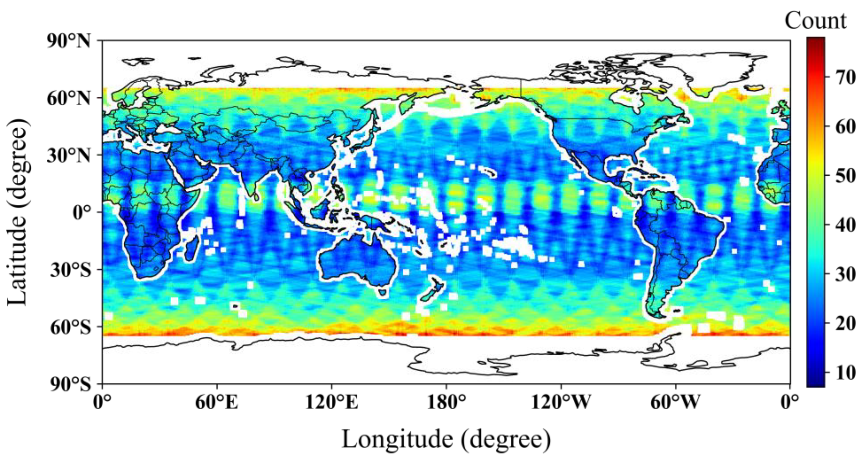
Figure 3.
Scatter plots of the predicted TPWs versus the ERA5 TPWs of the testing data (a) over sea surfaces and (b) over land surfaces.
Figure 3.
Scatter plots of the predicted TPWs versus the ERA5 TPWs of the testing data (a) over sea surfaces and (b) over land surfaces.
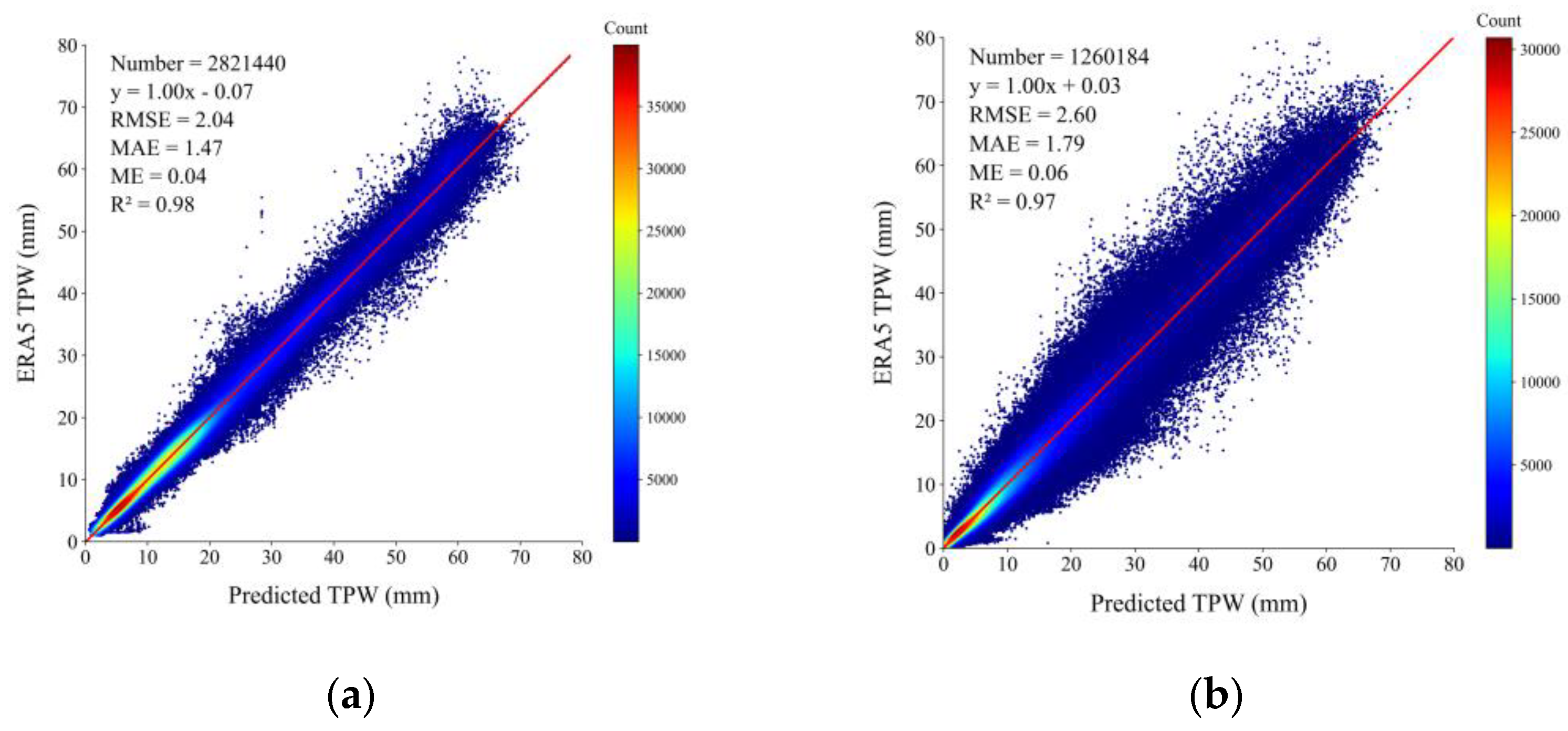
Figure 4.
Scatter plots of the predicted TPWs in this work versus the ERA5 TPWs over (a) the water bodies areas, (b) the snow and ice areas, (c) the barren or sparsely vegetated areas, (d) the croplands areas, (e) the urban and built-up areas, (f) the cropland/natural vegetation mosaic areas, (g) the evergreen needleleaf forest areas, (h) the evergreen broadleaf forest areas, (i) the deciduous needleleaf forest areas, (j) the deciduous broadleaf forest areas, (k) the mixed forest areas, (l) the closed shrublands areas, (m) the open shrublands areas, (n) the woody savannas areas, (o) the savannas areas, (p) the grassland areas, and (q) the permanent wetland areas.
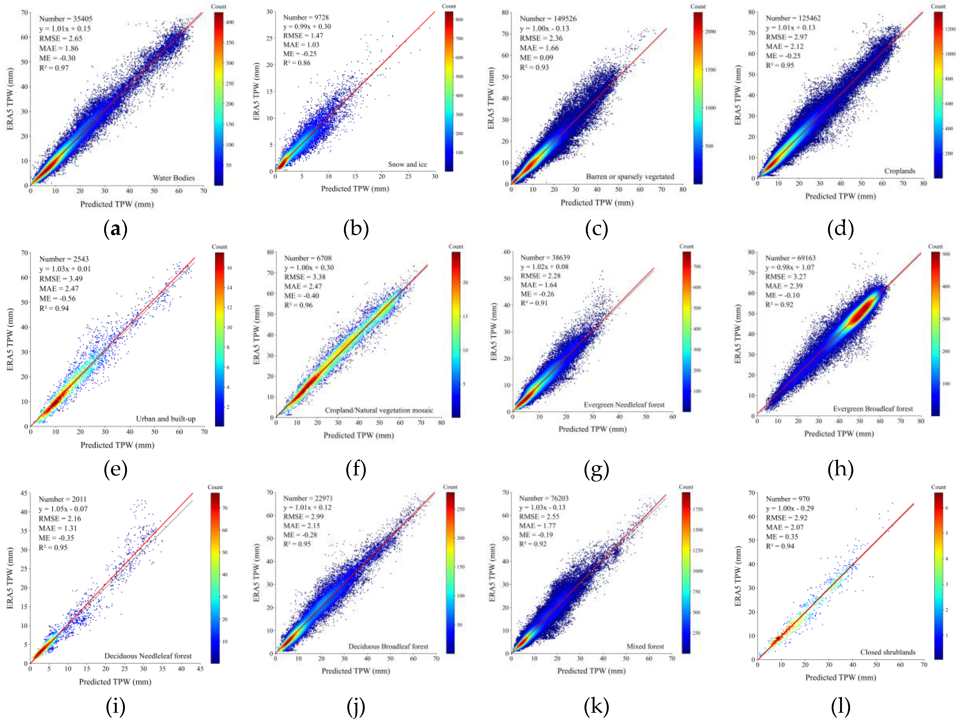
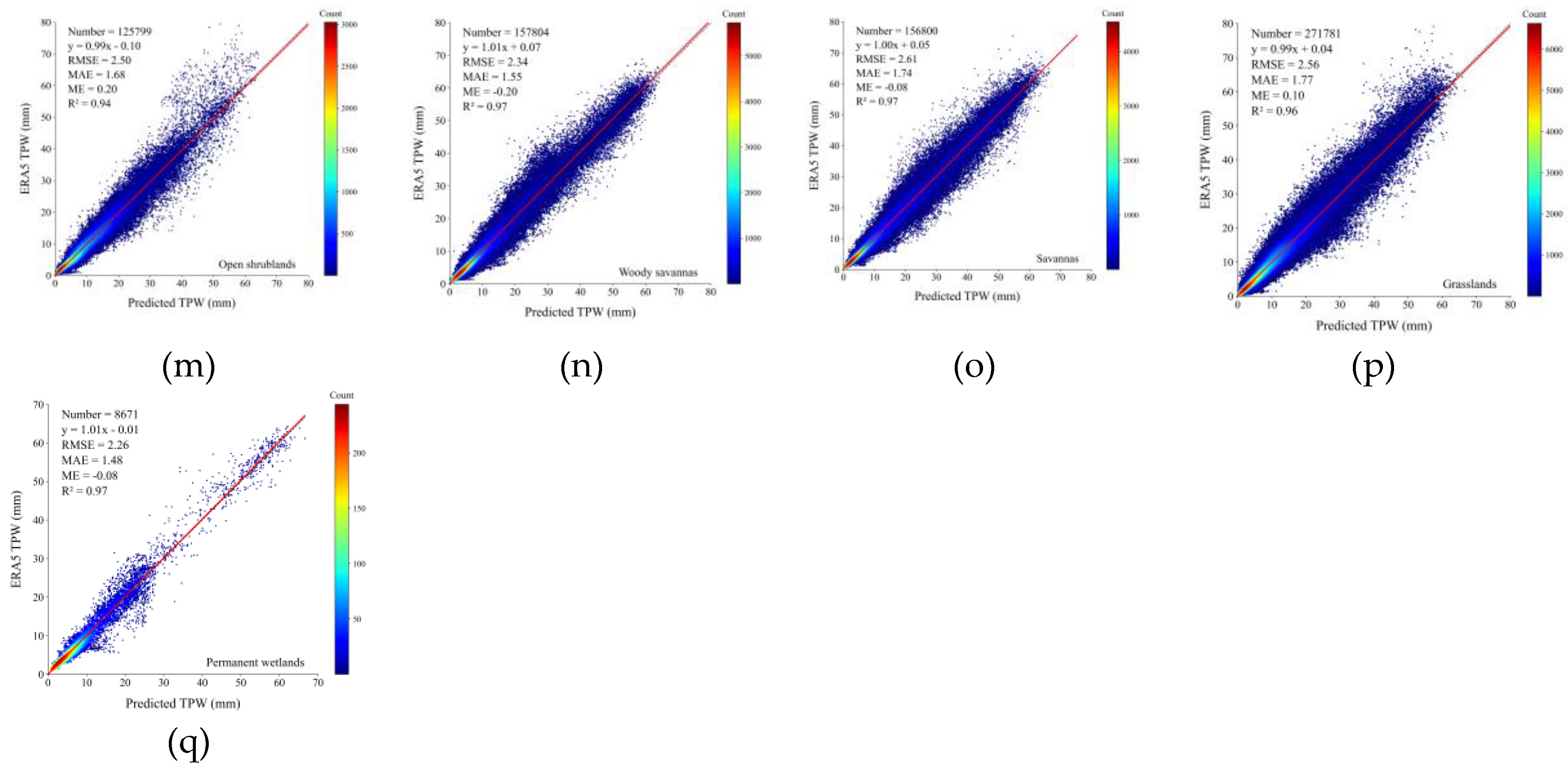
Figure 5.
SHapley Additive exPlanations (SHAP) values of the input features over (a) sea surfaces and (b) land surfaces (TBi denotes the brightness temperature in the MWHS-II channel i, while EiV and EiH stand for the land surface emissivities in the MWHS-II channel i at vertical and horizontal polarizations, respectively).
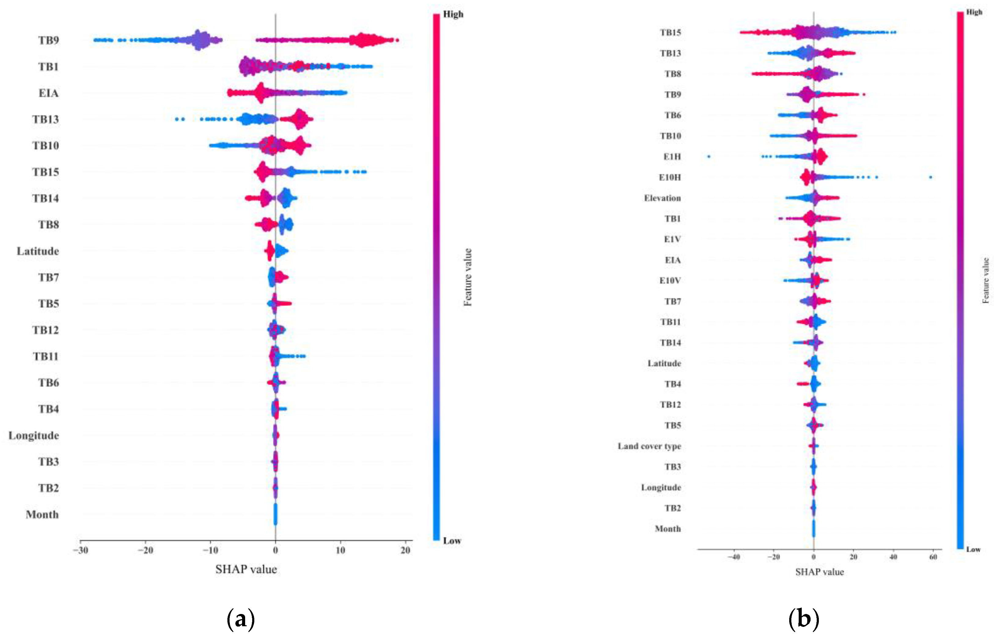
Figure 6.
Maps of the total precipitable water retrieved from the FY-3D MWHS-II data on (a) January 1, 2022, (b) April 1, 2022, (c) July 1, 2022, and (d) October 1, 2022.
Figure 6.
Maps of the total precipitable water retrieved from the FY-3D MWHS-II data on (a) January 1, 2022, (b) April 1, 2022, (c) July 1, 2022, and (d) October 1, 2022.
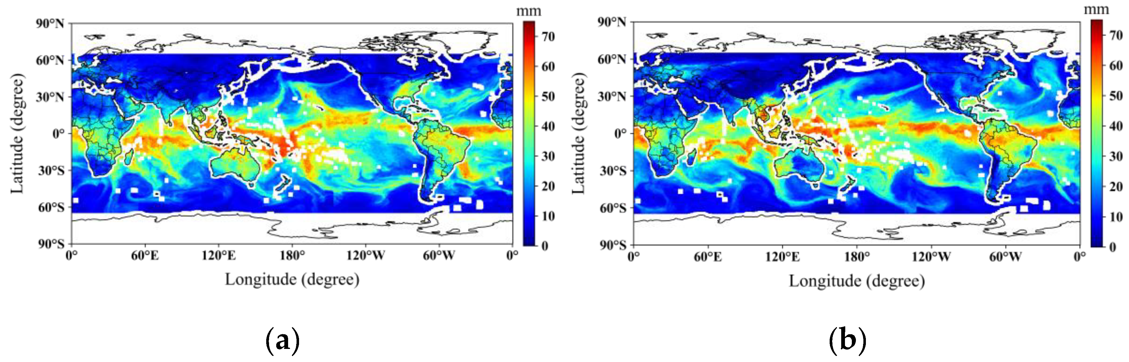
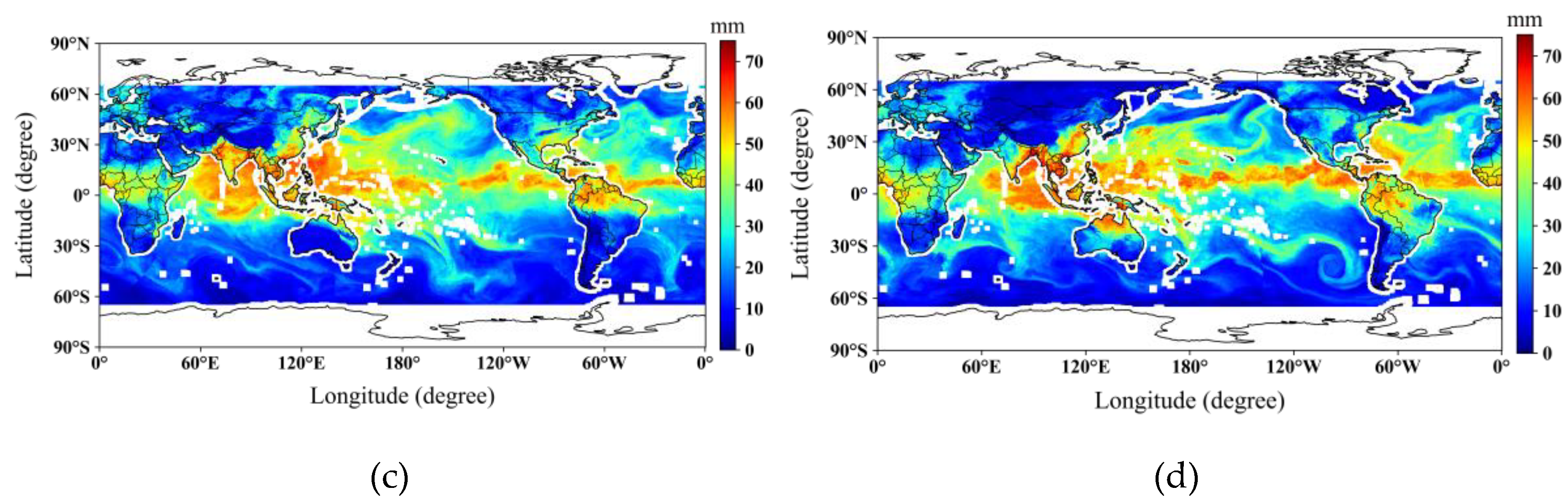
Figure 7.
The spatial distribution of the selected radiosonde stations.
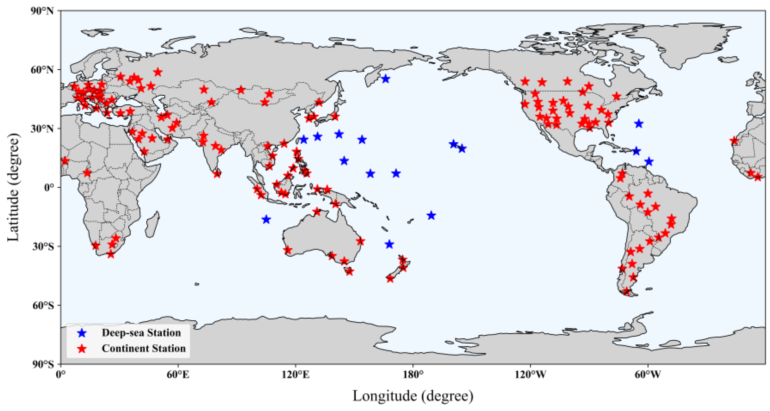
Figure 8.
Scatter plots of the TPWs retrieved in this work versus the radiosonde TPWs (a) over sea surface and (b) over land surfaces.
Figure 8.
Scatter plots of the TPWs retrieved in this work versus the radiosonde TPWs (a) over sea surface and (b) over land surfaces.
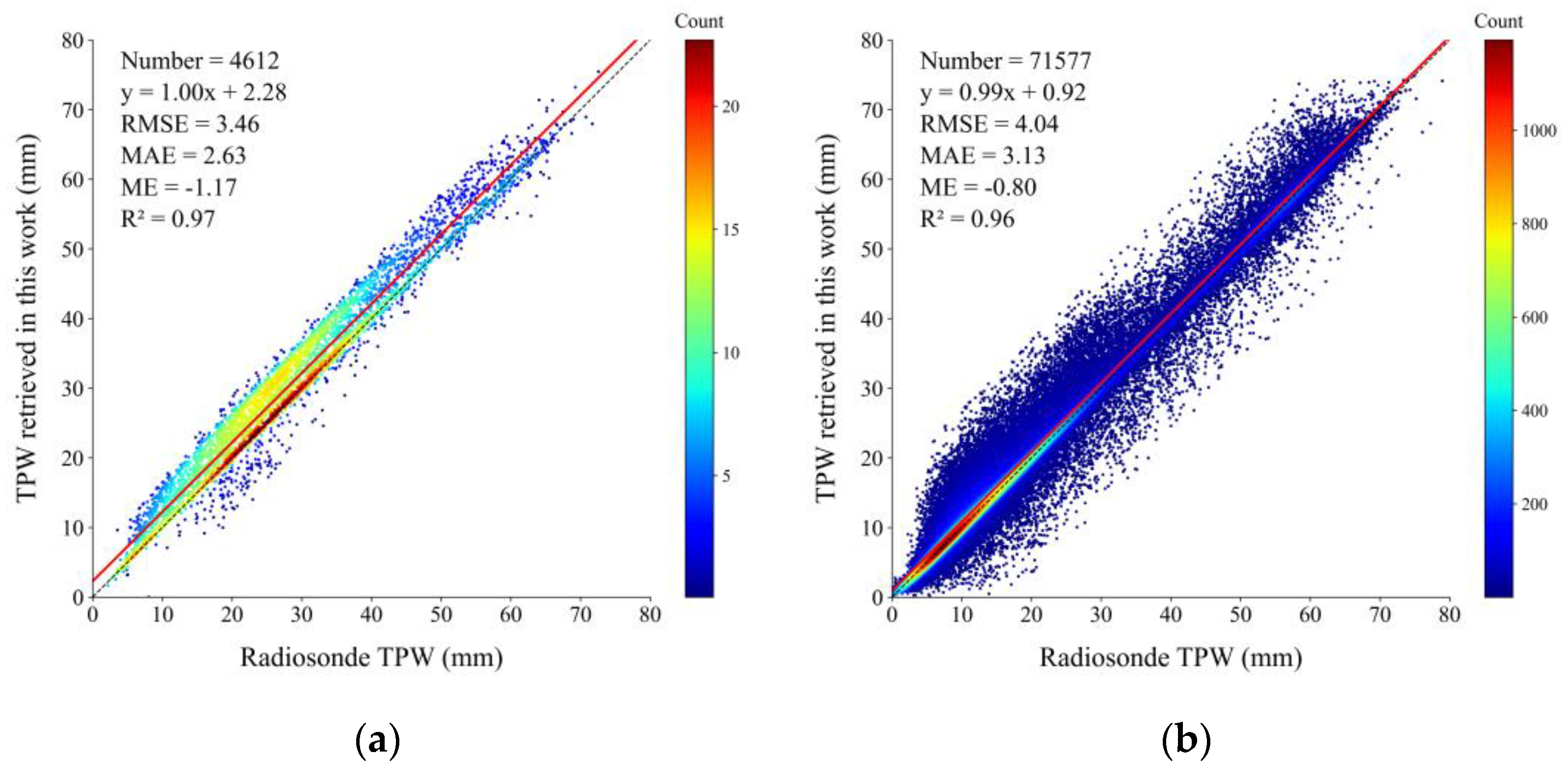
Figure 9.
Scatter plot of the F18 SSMIS TPWs versus the radiosonde TPWs.
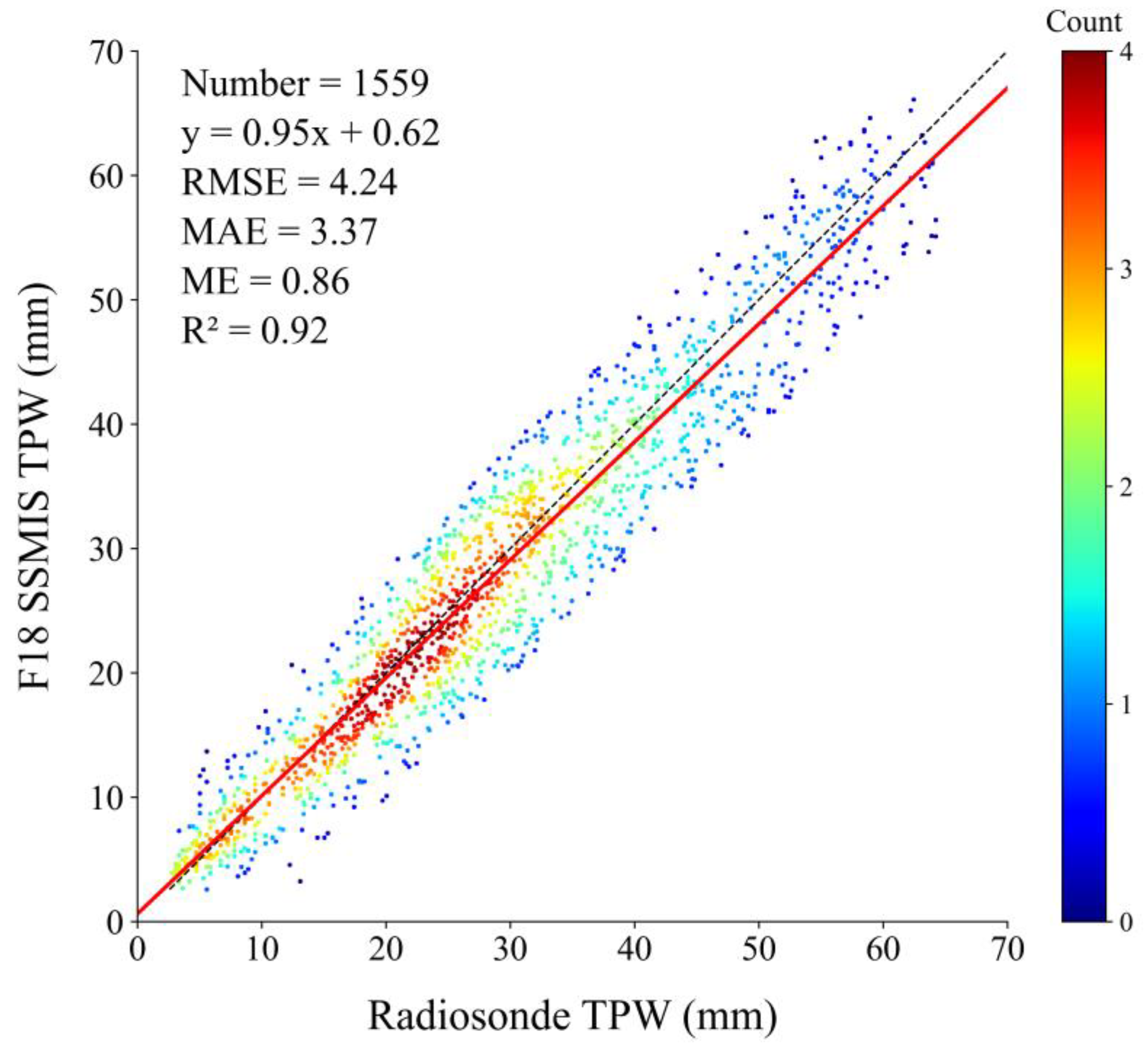

Table 1.
Instrument parameters of FY-3D MWHS-II.
| No. | Central frequency (GHz) |
Polarization | Bandwidth (MHz) |
NEΔT (K) |
Spatial resolution (km) |
|---|---|---|---|---|---|
| 1 | 89.0 | QH | 1500 | 1.0 | 30 |
| 2 | 118.75±0.08 | QV | 20 | 3.6 | 30 |
| 3 | 118.75±0.2 | QV | 100 | 2.0 | 30 |
| 4 | 118.75±0.3 | QV | 165 | 1.6 | 30 |
| 5 | 118.75±0.8 | QV | 200 | 1.6 | 30 |
| 6 | 118.75±1.1 | QV | 200 | 1.6 | 30 |
| 7 | 118.75±2.5 | QV | 200 | 1.6 | 30 |
| 8 | 118.75±3.0 | QV | 1000 | 1.0 | 30 |
| 9 | 118.75±5.0 | QV | 2000 | 1.0 | 30 |
| 10 | 150.0 | QH | 1500 | 1.0 | 15 |
| 11 | 183.31±1.0 | QV | 500 | 1.0 | 15 |
| 12 | 183.31±1.8 | QV | 700 | 1.0 | 15 |
| 13 | 183.31±3.0 | QV | 1000 | 1.0 | 15 |
| 14 | 183.31±4.5 | QV | 2000 | 1.0 | 15 |
| 15 | 183.31±7.0 | QV | 2000 | 1.0 | 15 |
Table 2.
Monthly distribution of the matching samples in 2022.
| Month | Number over sea surfaces | Number over land surfaces |
|---|---|---|
| 1 | 1195700 | 525927 |
| 2 | 1077674 | 487052 |
| 3 | 1258405 | 540884 |
| 4 | 1199367 | 518953 |
| 5 | 1202770 | 548763 |
| 6 | 1155894 | 521118 |
| 7 | 1021385 | 465599 |
| 8 | 1210438 | 537761 |
| 9 | 1189825 | 540628 |
| 10 | 1226708 | 542100 |
| 11 | 1176881 | 537094 |
| 12 | 1192158 | 535045 |
Table 3.
Comparison of the BPNNs in this work to other methods.
| Region | Method | ME | MAE | RMSE | MSLE | MAPE (%) | R2 |
|---|---|---|---|---|---|---|---|
| Sea | BPNN in this work | 0.04 | 1.47 | 2.04 | 0.01 | 8.64 | 0.982 |
| D-Matrix | 0.07 | 3.36 | 4.34 | 0.09 | 20.37 | 0.924 | |
| Ridge | 0.07 | 3.32 | 4.31 | 0.09 | 20.22 | 0.927 | |
| Lasso | 0.07 | 3.36 | 4.34 | 0.09 | 20.34 | 0.927 | |
| Physical | 0.00 | 3.32 | 4.33 | 0.09 | 24.61 | 0.916 | |
| RF | 0.07 | 2.87 | 4.03 | 0.05 | 18.73 | 0.943 | |
| SVM | 0.07 | 3.03 | 4.41 | 0.06 | 19.02 | 0.935 | |
| XGBoost | 0.03 | 1.97 | 2.71 | 0.02 | 10.76 | 0.976 | |
| Land | BPNN in this work | 0.06 | 1.79 | 2.60 | 0.03 | 15.53 | 0.967 |
| D-Matrix | 0.08 | 4.90 | 6.81 | 0.40 | 39.01 | 0.805 | |
| Ridge | 0.08 | 4.92 | 6.80 | 0.40 | 39.02 | 0.808 | |
| Lasso | 0.08 | 4.86 | 6.73 | 0.39 | 38.71 | 0.813 | |
| RF | 0.08 | 3.01 | 4.80 | 0.20 | 27.89 | 0.897 | |
| SVM | 0.09 | 3.20 | 4.92 | 0.20 | 29.19 | 0.871 | |
| XGBoost | 0.10 | 1.99 | 2.97 | 0.03 | 16.22 | 0.954 |
Disclaimer/Publisher’s Note: The statements, opinions and data contained in all publications are solely those of the individual author(s) and contributor(s) and not of MDPI and/or the editor(s). MDPI and/or the editor(s) disclaim responsibility for any injury to people or property resulting from any ideas, methods, instructions or products referred to in the content. |
© 2025 by the authors. Licensee MDPI, Basel, Switzerland. This article is an open access article distributed under the terms and conditions of the Creative Commons Attribution (CC BY) license (http://creativecommons.org/licenses/by/4.0/).
Copyright: This open access article is published under a Creative Commons CC BY 4.0 license, which permit the free download, distribution, and reuse, provided that the author and preprint are cited in any reuse.


