
Submitted:
12 July 2024
Posted:
14 July 2024
You are already at the latest version
Abstract
The use of low cost sensors has dramatically increased in recent years in all the engineering sectors. In the field of buildings and automotive, low cost sensors open very interesting perspectives, because they allow to monitor temperature and humidity distributions together with air quality, in a widespread and punctual way and allow control of all energy parameters. The main issue still open remains the validation of the measurements. In this work, we propose an innovative approach to verify the measurements given by some low-cost systems built ad hoc for automotive applications. Two independent low-cost measurement systems have been set to measure Particulate air Matter (PM) concentration, TVOC concentration, CO2 concentration, formaldehyde concentration, air temperature, relative humidity, pressure, air flow velocity and GPS position. These systems have been calibrated by the comparison with standard and certified sensors used by the regional authority of Emilia-Romagna region (ARPAE, Italy) for characterising the air-quality. The innovation of this approach lies in both the in-field comparison of low-cost and high quality sensors and the use of proper conversion approaches for mass concentration measurements. A quantitative analysis of the sensors performance is given, with a focus on effects of time-granularity, relative humidity, mass conversion from particle counts and size detection response. The results show that the low-cost sensors measurements of air temperature, relative humidity and particle number concentration are in a good agreement with high quality sensors measurements, with a strong impact of relative humidity on performance indicators. Overall, a good quality and consistency of the data among the sensors has been achieved.

Keywords:
air quality
; low cost sensors
; sensor validation
; pollutant concentration measurement
1. Introduction
Interest in air quality monitoring is gaining more and more attention from public authorities, companies and citizens for both outdoor and indoor environments [1,2]. Climate change, pollution and COVID-19 issues are well known air quality related topics very important in buildings, but also automotive sector is pushing the development of novel air quality standards. Several studies have underlined the relevance of particle counters in the determination of adverse health effect air pollution, thus suggesting that both particle number and mass concentrations should be measured [3].
In this context, the thorough diffusion of low-cost sensors is considered a promising technology for the improvement of spatial and temporal resolution of these measurements. Though, it must be noted that accuracy of data obtained from these devices is questionable if compared with reference measurements techniques and still matter of research [4]. Recent efforts in the development [5] and performance assessment [6] of these devices have been made, both at sensor and system level, underlining the importance of calibration for a reliable output. Belosi et al. [7] evaluated the performance of four optical particle counters (OPCs) with a standardized particle generator; they found good results for total particle number concentration, while aerosol size distribution and average particle density must be improved as they relate closely with particle mass concentration [7]. Conversion from particle to mass concentration represents a crucial task if a good performance of OPCs is desired. A study from Franken et al. compared different conversion methods with a focus on PM2.5 mass concentrations [8]. They found that while good correlations (Pearson) are possible with the developed method, other methods resulted in an underestimation of particle mass concentration if compared with gravimetric data.
However, many manufacturers perform only calibration in environmental chambers with controlled process parameters. The latter being a necessary but not sufficient procedure, thus indicating field calibration as a mandatory task, particularly if the acquisition system needs to be relocated. Recent studies have investigated the performance of different calibration approaches, ranging from simple linear regression to machine learning (ML) techniques [9]. The selection of the best method is strongly case specific and must be performed considering experiment setup, sensor selection, site location and measurement duration. An example of field calibration is given by Dinoi et al. [10]. The work reports a comparison between three OPCs against a urban background reference station; showing that effect of relative humidity (RH) is considerable and should be compensated, especially for mass concentration evaluation. On the contrary, Zou et al. investigated the relationship between environmental variables such as air temperature and RH on eight low-cost particle sensor output [11], but using a controlled chamber and common particle sources. On one hand, they found no significant effect of temperature, on the other hand RH has an impact on magnitude of particle readings but still may be compensated with a simple RH-based calibration as the output correlates well with reference instrumentation.
If a vehicle cabin IAQ LCSoS is considered as mobile, therefore continuously relocated system; the robustness of its field calibration method becomes of paramount importance. Existing assessment techniques rely on relevant factors probability distribution changes that allow performance prediction of field calibration models, but still co-located reference measurements involving several months are required [12]. Main aim of this work is to build and perform at system scale a fast field calibration of a low-cost SoS based on Arduino hardware; effects of environmental variables on particle-related output variables are also discussed. Secondly, we aim to assess the performance at sensor scale, of SPS30, a quite new and powerful device that has still poor literature support. Third aim is to demonstrate the metrological capabilities of a LCSoS in the automotive field, thus enabling its operation in transient, non-uniform and moving environments such as vehicle cabins [13].
2. Materials and Methods
2.1. Arduino-Based Sensor Systems
In this section, in order to describe the complex in-field methodology deployed for the low-cost sensor validation, the following subsections are shown. First, two low cost sensor arrangements ad hoc built for the characterisation of air quality are introduced. Then, the site with the reference calibrated instrumentation used by the regional authority ARPAE is described. The details of the measurement campaign with the low-cost sensors arrangement in the reference station is then explained. Finally, the methodology used to acquire and manipulate data for the comparison is discussed.
Two independent measurement systems (IS,ES) based on Arduino Mega 2560 were built for the measurement of environmental parameters [14,15]. The systems have an on-board Real Time Clock (RTC), a data logger on flash memory, a fan and a TFT display. The RTC clocks of the two systems are constantly synchronised thanks to time data received from the GPS module.
Both systems can measure Particulate air Matter (PM) concentration (Sensirion SPS30 sensor), air TVOC concentration (Sensirion SGP30 sensor), air CO2 concentration (Winsen MH-Z19B non-dispersive infrared sensor), concentration formaldehyde (Winsen ZE08 sensor), air temperature, relative humidity and pressure (Bosch Sensortec BME280 sensor), air flow velocity (hot wire analog sensor) and GPS position. The systems are equipped with a fan that conveys air inside the device enclosure, where CO2 and formaldehyde sensors are mounted, while the SPS30 sensor is equipped with its built-in fan. Both systems independently sampled data at 10-second intervals. All digital sensors used in the measurement device include a microcontroller that implements optimization and self-calibration algorithms. Among all the quantities measured by the low-cost SoS, only those overlapping with the reference instrumentation are considered in this study and reported in Table 1 together with available daily values from the closest ARPA reference station. The quantities subset can be related to two of the sensors installed in the LCSoS, namely the BME280 and SPS30.
The BME280 is a high linearity and high accuracy air temperature, humidity and pressure sensor. Respectively, its pressure operation range is 300–1100, -45∘C–85∘C for temperature, and 0–100 for humidity. It features an extremely fast response time of 1 , thus enabling a consistent oversampling if compared with the current application time granularity [16].
The laser scattering-based SPS30 PM sensor allows mass concentration and number concentration sensing. The sensor encapsulates a miniaturised fan and a High Efficiency Particulate Air (HEPA) filter to reduce the optical particle contamination; it also runs its fan at full speed for 10 seconds every 7 days and at startup as an automatic cleaning procedure. Mass concentration measurement range: 0 to 1000 . As discussed in [17] and [18], the SPS30 is an optical particle counter (OPC) optimised for PM2.5 and smaller particle analysis. In fact, Sensirion PM sensors are calibrated using regularly maintained and aligned with high-end reference instruments (e.g., the TSI Optical Particle Sizer Model 3330 or the TSI DustTrak™ DRX 8533) only for particles size. Moreover, as reported in the sensor specification statement from the producer, PM4 and PM10 outputs are not directly measured but estimated from smaller particle counts using typical aerosol profiles. This behaviour is also confirmed by the SPS30 detection range being identical for 1 and above, thus warning about the use of the sensor for bigger particles sensing [19].
2.2. Measurement Site and Reference Instrumentation
The reference site is located in northern Italy, inside the research area of CNR in Bologna (see Figure 1). The site is classified as urban background station. Measurements from this instrumentation will be referenced as ARPAE System (AS) in the following sections. The reference measurements chosen were performed by an OPC FAI (Multichannel Monitor, FAI Instrument - Rome, Italy) which classifies particles in 8 size intervals from 0.28 g to 10 g and is equipped with a 10 g inlet head and operates with a 1 l/min flow rate. The measurement principle is the laser scattering: the sensor uses a 35mW laser diode as the light source and a mirror collecting system elliptical. The light diffused by the particles and collected by the elliptical mirror is concentrated in a photodiode that converts light energy into electric current. The air sample is transferred to the mixing chamber where it is diluted with clean and dehumidified air (free of particles and with low humidity level relative): a smart heater placed in the diluter along the mixing chamber that is automatically operated only when needed. OPC Multichannel Monitor is therefore equipped with a temperature and relative humidity sensor in the external environment, protected from direct solar radiation and from rain, and one inside the instrument to detect temperature and humidity relative to the diluted sampling air that passes through the Laser Sensor. Furthermore, the FAI instrument implements a tool (Zero Test) to verify that the sensor provides “zero” counts in the presence of particle-free air. This test also makes it possible to verify that there is no infiltration of external air in the dilution circuit (in the first hour 15 test zero minutes are dropped every day). OPC FAI also provides measurement of estimated PM (PM1, PM2.5, PM10) and is integrated with a Swam Dual Channel (SWAM 5a DC, FAI Rome, Italy) that determines PM2.5 and PM10 daily mass concentration with -ray attenuation method using a low volume (2.3m3/h). The integration gives an automatic correction with real mass values supplied by SWAM DC with self-learning procedure. Conversion from number to PM mass concentration is performed using the algorithms provided by the FAI constructors.
2.3. Measurement Campaign with Sensors Arrangement
Experimental campaign started 2021-05-18 at 12.00 and finished 2021-05-21 at 12.00. Total test duration was 3 full days, thus providing enough points for the chosen temporal resolution of 1 . The latter was defined according to the typical time resolution of the two classes of instruments. Reference instrumentation provides data with a sample rate of 1 , but verified measures are usually provided as a daily average. On the other hand, low-cost SoS can output data at 10 sample rate. Given the different time granularity of the two systems, we opted for a 1 time averaging, which gives a total of 72 samples calculated averaging 4320 minutely samples available ( 26000 for the LCSoS). Nevertheless, a 24-h average of data measured during the parallel measurement with the reference method shall always be calculated and reported [20]. Only two central days of the measurement period are suitable for such a comparison given in Table 1, also because a daily average should be considered valid only if 75 of the hours are covered; this is not the case for first and last day.
The experimental setup has been built balancing the needs of the experimental campaign with those of the sensors. To ensure the best performance of the SoS we extended the design and assembly guidelines provided by Sensirion for the SPS30 to the whole system. The most important being:
- A good coupling with ambient air and a proper exposition to external conditions
- Avoidance of exposure to direct sunlight or external heat sources
The low-cost SoS was placed near the sampling inlet of the reference station. A 4 thick thermal insulating layer has been used at the bottom and top to provide shading and thermal insulation, a pierced plastic shell was used to connect the two planes thus providing support for the top plane but allowing a good air exchange in the sampling volume (see Figure 2).
2.4. Methods Used to Acquire and Manipulate Data
The two Arduino Mega 2560-based acquisition systems were programmed using the standard Arduino IDE. The following specific libraries were used for the sensors mentioned in the previous section: sps30.h, DallasTemperature.h, Adafruit_SGP30.h, Adafruit_BME280.h, DFRobotHCHOSensor.h and TinyGPS++.h. Each acquired data is saved on an SD memory card together with a time reference, synchronised in both systems by the reference clock signal received by GPS from both systems.
An Exploratory Data Analysis (EDA) approach was applied to the data-set, thus providing insights to the problem definition and model imposition only after analysing the data [21]. The open source tools chosen for the EDA were python 3.8 and several scientific computing libraries (pandas, matplotlib, numpy and scipy above all). Procedures used are more graphical than quantitative as required by EDA approach.
When comparing multiple particle sensing devices, their builtin size buckets must be considered. Reference instrumentation often comes with a higher size resolution than LCSs, and an accurate grouping of size bins becomes inevitable [22]. Table 2 shows the grouping adopted in this study for EDA and confirmatory data analysis, while Figure 3 exhibits channel splitting for reference and low-cost instrumentation respectively.
3. Results
A qualitative overview of the SoS performance is shown in Figure 4 and Figure 6 for the whole test duration. Five variables of interest have been selected considering their overall correlation with particulate matter mass concentration as shown in Figure 5. Conversely, variables that showed a poor Pearson’s correlation coefficient R have been disregarded. The two LCS show an excellent consistency between themselves as already stated in previous studies [19]. A good agreement on temperature data is appreciable. Particular attention must be paid to RH as it has a direct impact on sensing mechanism of OPCs, and poor performance at full-scale raises an alert. Regarding PM, correlation seems to decrease ranging from smaller particle size to bigger ones. A quantitative analysis of the SoS performance is given in the following sections, with a focus on effects of time-granularity, relative humidity, mass conversion from particle counts and size detection response. Prior to that, an accent must be put on the small PM values observed during the test, thus making the instrumentation operate on the low-end of the measurement range.
3.1. Time Granularity
Choosing the best time granularity for data analysis is not a simple task. Some authors suggest to define it in the EDA phase and before the data analysis is performed; moreover they warn against the use of statistical significance as a selection metric for time granularity as it can lead to misinterpretation of results [23,24]. In this study, the following factors are considered: total test duration, different time scales between SoS and official data, field of application. A compromise is needed between the time scale which is best for automotive application (minutely or less) and the the time scale of validated data from ARPAE (daily values with a 6 months validation process). A common approach for ambient validation of PM data is to perform the analysis on hourly averaged results [22].
3.2. RH Sensitivity Analysis
It is well known that among the factors influencing PM measurements, RH plays a major role. This is true to the point that reference gravimetric methods rely on a controlled sampling process in terms of temperature an relative humidity of the air sample across the filter. These methods are not applicable for LCS and the definition of a RH correction factor is quite common [9]. In order to evaluate the influence of RH on the sensor response, we can look at Figure 7 and Figure 8, which show scatter and box plots of number and mass concentration for particle size. RH values have been aggregated in four uniformly spaced bins, thus providing insights on statistical dispersion in each RH bin. Despite being in agreement among themselves, LCS IS and ES have a wider inter quartile range (IQR) toghether with a greater number of outliers; the worst scenario corresponds with values of RH above 75 . Similar consideration can be drawn from Figure 9, which reports the same quantities but without binning. It is noticeable an increased dispersion of the data with growing RH values; also in this case higher particle counts associated high RH values do not fit well with the reference system AS. It should be noted that the dispersion of data points increases in the transition from particle count to particle mass, probably due to the theoretical mass conversion adopted in OPCs. Further results dealing with mass conversion will be presented in the following section.
In order to quantify the impact of the predictor variable RH on the response variable NC2.5, an univariate linear regression has been adopted. Results from the ordinary least squares (OLS) analysis are reported in Figure 10, showing again that the sensor performance degrades at high RH values. The improvement in approaches 0.11 when values of RH above 50 are dropped from the data-set.
3.3. Mass Conversion Correction
Before delving into mass conversion results, it is worth recalling how mass concentration can be calculated from particle counts, together with associated challenges. Mass conversion adopted in OPC is based on the assumption that particle are spherical and with common density in each size bin; in practice this is made according to the following equation [8], based in the assumption that particles are spherical and with a single density in each size bin:
where i is the particle size bin, is the mass concentration in /3, is the particle average density, is the median particle diameter in and is number concentration for a given size bin. It is immediately clear from equation 1, that a good estimation of as input parameter for the conversion algorithm is crucial. A widely adopted value is /cm3 [25], but its variability in time and space must be considered carefully after relocation. Mass conversion based on equation 1 requires to be known in each size bin; an information not always available for LCSs. Sensirion SPS30 provides a typical particle size output that is correlated with weighted average of the number concentration bins measured with a reference particle sizer. Substituting in equation 1 leads to the calculation of a typical particle mass, which can be used to perform a manual conversion whose results are displayed in Figure 11. Pearson correlation between LCS and AS increases from to in this case. An alternative approach proposed in this study relies instead on the calculation of a constant ratio between mass and particle counts in the chosen bin from the reference instrumentation data. The defined quantity can be seen as an average particle mass used to calculate a corrected mass concentration from the number concentration of the LCS. The latter being a direct and more reliable measurement, as shown in the previous section. Figure 11, contains three plots that clarify the correction procedure. With this method, the Pearson correlation of PM values between LCS and AS increases from to , a value again comparable with the correlation between particle number concentration.
4. Discussion
In this study, an innovative calibration procedure to qualify low-cost systems of sensors capable of a high spatio-temporal resolution through a field comparison against reference instrumentation operated by ARPAE is shown. Main factors influencing particle sensors output were first measured and then identified with an EDA approach; their impact in terms of data quality and correlation with reference instrumentation was also analyzed. The LCSoS is constituted by an Arduino open-hardware platform and commercially available LCSs. Open-source software tools were used for acquisition and post-processing algorithms, thus further supporting the repeatability of the experiment and spreadability of the device. Results show that the system has a relatively good performance with respect to air temperature, relative humidity and smaller particle number concentration () with coefficient of determination approaching for the reduced data set, as also confirmed in previous studies [22]; RH has a strong impact on performance indicators and correction techniques are strongly recommended [11,12]. If few works were found to deal with Sensirion SPS30, even fewer were dealing with mass conversion [8,26]. In the last part of this work we compared three conversion approaches: the sensor builtin output, a mass concentration calculated from particle concentration and a mass concentration corrected according to reference instrumentation data. Both techniques provide an improvement of the overall Pearson R ranging from to on the PM10 value. It is also important to underline that PM correlation with daily values from the verified ARPAE network are quite poor; on the other hand, a good quality and consistency of the data among LCSoS was observed. An IAQ monitoring system like the one proposed in this research can be subject to frequent relocation (moving measurement), this can lead to calibration issues that must be addressed. More sophisticated calibration models (ML) are supposed to provide more effective calibration procedures, but require longer training [6,9] and might result in unpractical methods for automotive and high spatio-temporal resolution applications. For this reason we opted for a short measurement period of three days and well established yet simple performance assessment procedures. Further research on these aspects must be carried on, as useful insight are possible from LCSs, but their reliability is still far from reference instrumentation.
Abbreviations
| ARPAE | Agenzia regionale per la prevenzione, l’ambiente e l’energia |
| dell´Emilia-Romagna | |
| AS | ARPAE System of Sensors |
| BEV | Battery Electric Vehicle |
| EDA | Exploratory Data Analysis |
| ES | Low cost measurement system 1 |
| IAQ | Internal Air Quality |
| IS | Low cost measurement system 2 |
| LCS | Low Cost Sensor |
| ML | Machine Learning |
| NC | Number Concentration |
| OLS | Ordinary Least Squares |
| OPC | Optical Particle Counter |
| PM | Particulate Matter |
| RH | Relative Humidity |
| SoS | System of Sensors |
References
- Commission), J.R.C.E.; Borowiak, A.; Barbiere, M.; Kotsev, A.; Karagulian, F.; Lagler, F.; Gerboles, M. Review of sensors for air quality monitoring; Publications Office of the European Union: LU, 2019. [Google Scholar]
- Settimo, G.; Manigrasso, M.; Avino, P. Indoor Air Quality: A Focus on the European Legislation and State-of-the-Art Research in Italy. Atmosphere 2020, 11, 370. [Google Scholar] [CrossRef]
- Tittarelli, A.; Borgini, A.; Bertoldi, M.; De Saeger, E.; Ruprecht, A.; Stefanoni, R.; Tagliabue, G.; Contiero, P.; Crosignani, P. Estimation of particle mass concentration in ambient air using a particle counter. Atmospheric Environment 2008, 42, 8543–8548. [Google Scholar] [CrossRef]
- M. Gerboles.; L. Spinelle.; A. Borowiak. Measuring air pollution with low-cost sensors, 2017.
- Alfano, B.; Barretta, L.; Del Giudice, A.; De Vito, S.; Di Francia, G.; Esposito, E.; Formisano, F.; Massera, E.; Miglietta, M.L.; Polichetti, T. A Review of Low-Cost Particulate Matter Sensors from the Developers’ Perspectives. Sensors 2020, 20, 6819. [Google Scholar] [CrossRef] [PubMed]
- Zauli-Sajani, S.; Marchesi, S.; Pironi, C.; Barbieri, C.; Poluzzi, V.; Colacci, A. Assessment of air quality sensor system performance after relocation. Atmospheric Pollution Research 2021, 12, 282–291. [Google Scholar] [CrossRef]
- Belosi, F.; Santachiara, G.; Prodi, F. Performance Evaluation of Four Commercial Optical Particle Counters. Atmospheric and Climate Sciences 2013, 3, 41–46. [Google Scholar] [CrossRef]
- Franken, R.; Maggos, T.; Stamatelopoulou, A.; Loh, M.; Kuijpers, E.; Bartzis, J.; Steinle, S.; Cherrie, J.W.; Pronk, A. Comparison of methods for converting Dylos particle number concentrations to PM2.5 mass concentrations. Indoor Air 2019, 29, 450–459. [Google Scholar] [CrossRef] [PubMed]
- Liang, L. Calibrating low-cost sensors for ambient air monitoring: Techniques, trends, and challenges. Environmental Research 2021, 197, 111163. [Google Scholar] [CrossRef] [PubMed]
- Dinoi, A.; Donateo, A.; Belosi, F.; Conte, M.; Contini, D. Comparison of atmospheric particle concentration measurements using different optical detectors: Potentiality and limits for air quality applications. Measurement 2017, 106, 274–282. [Google Scholar] [CrossRef]
- Zou, Y.; Clark, J.D.; May, A.A. A systematic investigation on the effects of temperature and relative humidity on the performance of eight low-cost particle sensors and devices. Journal of Aerosol Science 2021, 152, 105715. [Google Scholar] [CrossRef]
- De Vito, S.; Esposito, E.; Castell, N.; Schneider, P.; Bartonova, A. On the Robustness of Field Calibration for Smart Air Quality Monitors. Sensors and Actuators B: Chemical 2020, 310, 127869. [Google Scholar] [CrossRef]
- Russi, L.; Guidorzi, P.; Pulvirenti, B.; Semprini, G.; Aguiari, D.; Pau, G. Air quality and comfort characterisation within an electric vehicle cabin. 2021 IEEE International Workshop on Metrology for Automotive (MetroAutomotive), 2021, pp. 169–174. [CrossRef]
- Kondaveeti, H.K.; Kumaravelu, N.K.; Vanambathina, S.D.; Mathe, S.E.; Vappangi, S. A systematic literature review on prototyping with Arduino: Applications, challenges, advantages, and limitations. Computer Science Review 2021, 40, 100364. [Google Scholar] [CrossRef]
- Kumar Sai, K.B.; Mukherjee, S.; Parveen Sultana, H. Low Cost IoT Based Air Quality Monitoring Setup Using Arduino and MQ Series Sensors With Dataset Analysis. Procedia Computer Science 2019, 165, 322–327. [Google Scholar] [CrossRef]
- Sensortec, B. BME280 Combined humidity and pressure sensor. Bosch Sensortec 2018. [Google Scholar]
- Li, J.; Li, H.; Ma, Y.; Wang, Y.; Abokifa, A.A.; Lu, C.; Biswas, P. Spatiotemporal distribution of indoor particulate matter concentration with a low-cost sensor network. Building and Environment 2018, 127, 138–147. [Google Scholar] [CrossRef]
- Tryner, J.; Mehaffy, J.; Miller-Lionberg, D.; Volckens, J. Effects of aerosol type and simulated aging on performance of low-cost PM sensors. Journal of Aerosol Science 2020, 150, 105654. [Google Scholar] [CrossRef]
- Kuula, J.; Mäkelä, T.; Aurela, M.; Teinilä, K.; Varjonen, S.; González, Ó.; Timonen, H. Laboratory Evaluation of Particle-Size Selectivity of Optical Low-Cost Particulate Matter Sensors. Atmospheric Measurement Techniques 2020, 13, 2413–2423. [Google Scholar] [CrossRef]
- ISO. BS ISO 16000-37:2019. Indoor Air - Part 37: Measurement of PM_{2,5} mass concentration; BSI Standards Publication, 2019.
- Guthrie, W.F. NIST/SEMATECH e-Handbook of Statistical Methods (NIST Handbook 151), 2020. type: dataset. [CrossRef]
- Kelly, K.E.; Whitaker, J.; Petty, A.; Widmer, C.; Dybwad, A.; Sleeth, D.; Martin, R.; Butterfield, A. Ambient and Laboratory Evaluation of a Low-Cost Particulate Matter Sensor. Environmental Pollution 2017, 221, 491–500. [Google Scholar] [CrossRef] [PubMed]
- Wakim, N.I.; Braun, T.M.; Kaye, J.A.; Dodge, H.H.; Orcatech, F. Choosing the Right Time Granularity for Analysis of Digital Biomarker Trajectories. Alzheimer’s & Dementia: Translational Research & Clinical Interventions 2020, 6, e12094. [Google Scholar] [CrossRef]
- Ma, Y.; Zhu, W.; Yao, J.; Gu, C.; Bai, D.; Wang, K. Time Granularity Transformation of Time Series Data for Failure Prediction of Overhead Line. Journal of Physics: Conference Series 2017, 787, 012031. [Google Scholar] [CrossRef]
- Weijers, E.P.; Khlystov, A.Y.; Kos, G.P.A.; Erisman, J.W. Variability of Particulate Matter Concentrations along Roads and Motorways Determined by a Moving Measurement Unit. Atmospheric Environment 2004, 38, 2993–3002. [Google Scholar] [CrossRef]
- Zikova, N.; Hopke, P.K.; Ferro, A.R. Evaluation of New Low-Cost Particle Monitors for PM2.5 Concentrations Measurements. Journal of Aerosol Science 2017, 105, 24–34. [Google Scholar] [CrossRef]
Figure 1.
Location of the reference station site in Bologna, decimal degrees (DD): (44.523698,11.340034).
Figure 1.
Location of the reference station site in Bologna, decimal degrees (DD): (44.523698,11.340034).
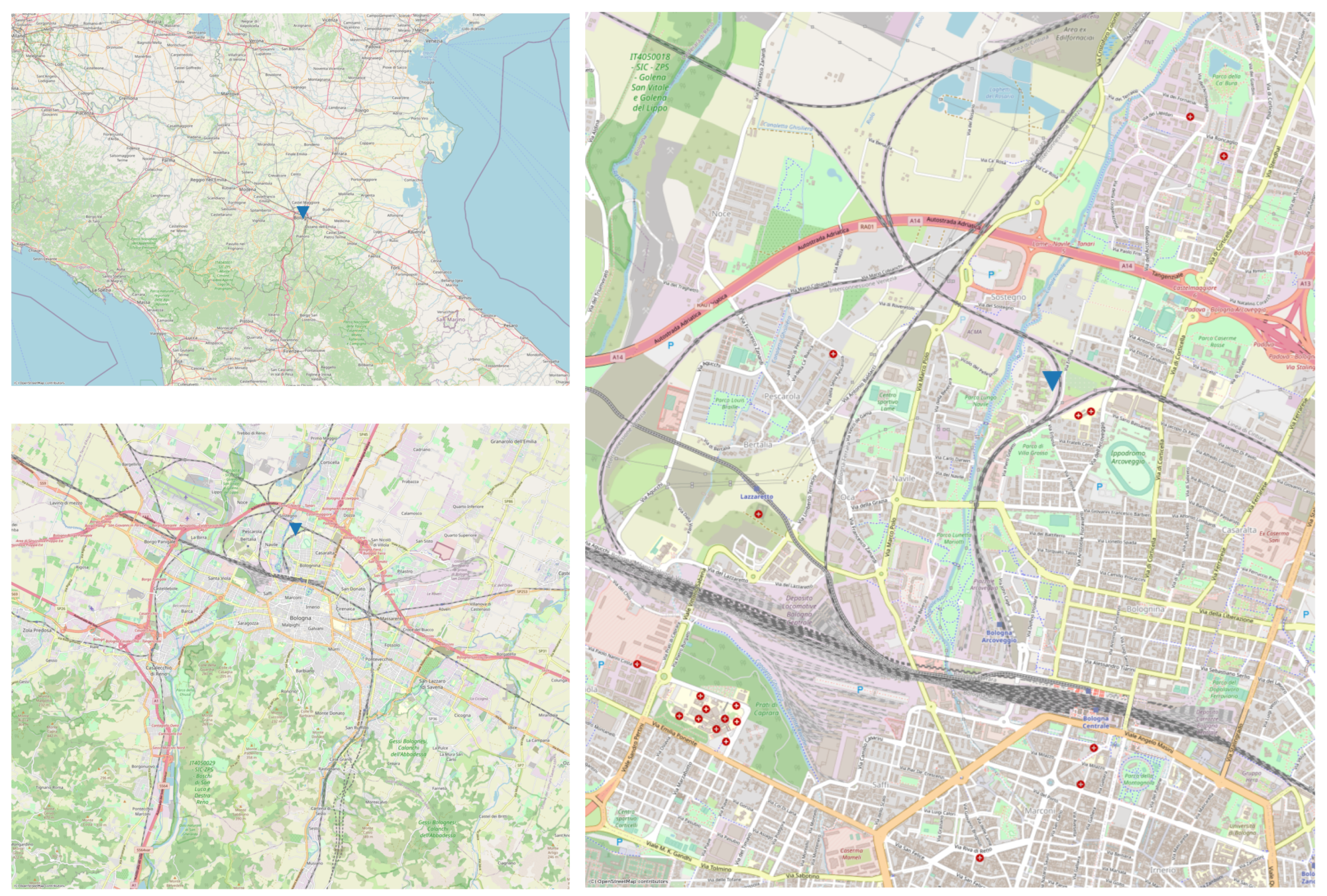
Figure 2.
Experimental setup for the LCSoS on the reference station roof.

Figure 3.
AS row buckets in 8 size channels Figure 3 and IS row buckets in 5 size channels Figure 3.
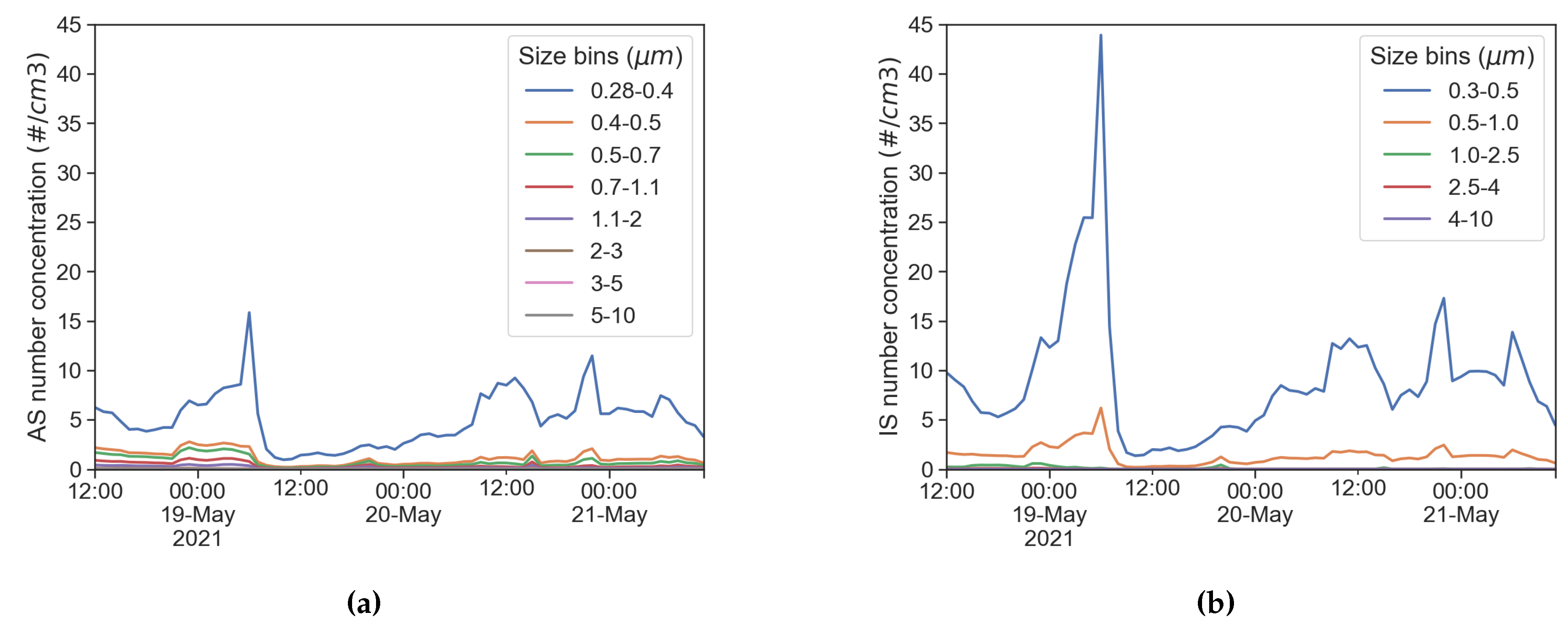
Figure 4.
Comparison between hourly data acquired from the two LCS (IS,ES) and from reference instrumentation (AS). Variables of interest are air temperature, relative humidity, PM1, PM2.5, PM10.
Figure 4.
Comparison between hourly data acquired from the two LCS (IS,ES) and from reference instrumentation (AS). Variables of interest are air temperature, relative humidity, PM1, PM2.5, PM10.
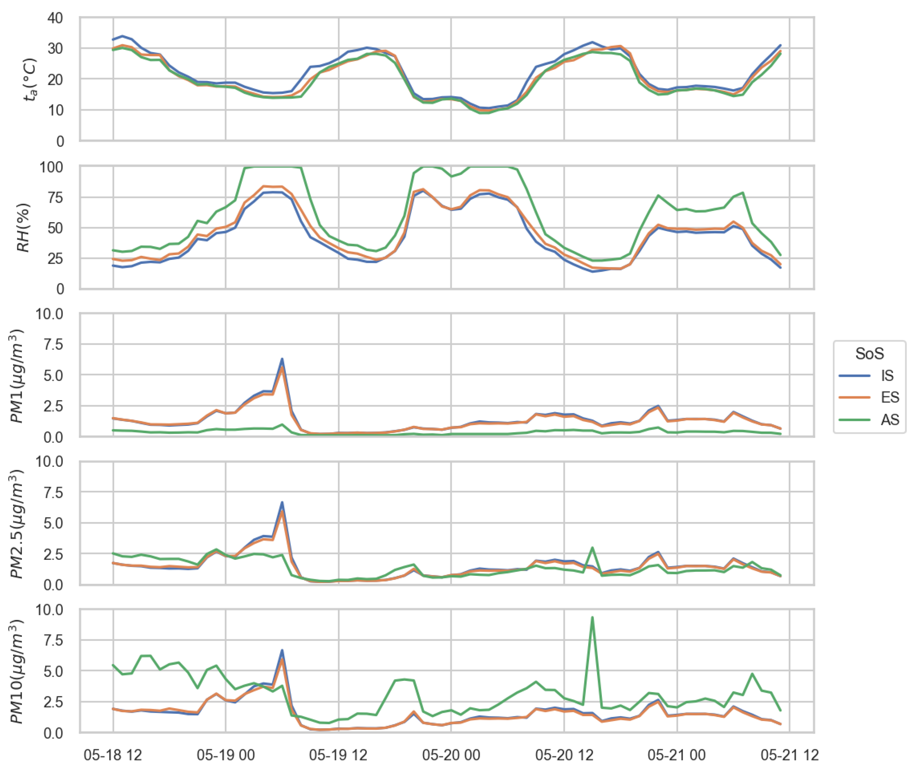
Figure 5.
Global correlation heatmap.
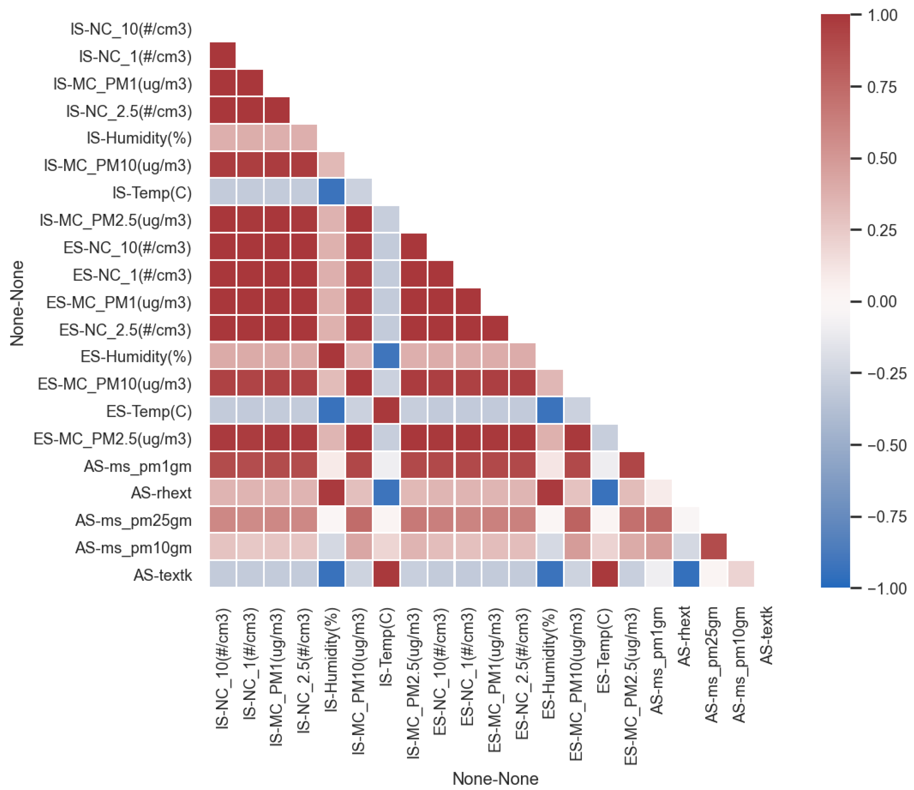
Figure 6.
Univariate kernel density estimation plots (diagonal) and bivariate scatter plots (off diagonal) of , , and distributions.
Figure 6.
Univariate kernel density estimation plots (diagonal) and bivariate scatter plots (off diagonal) of , , and distributions.
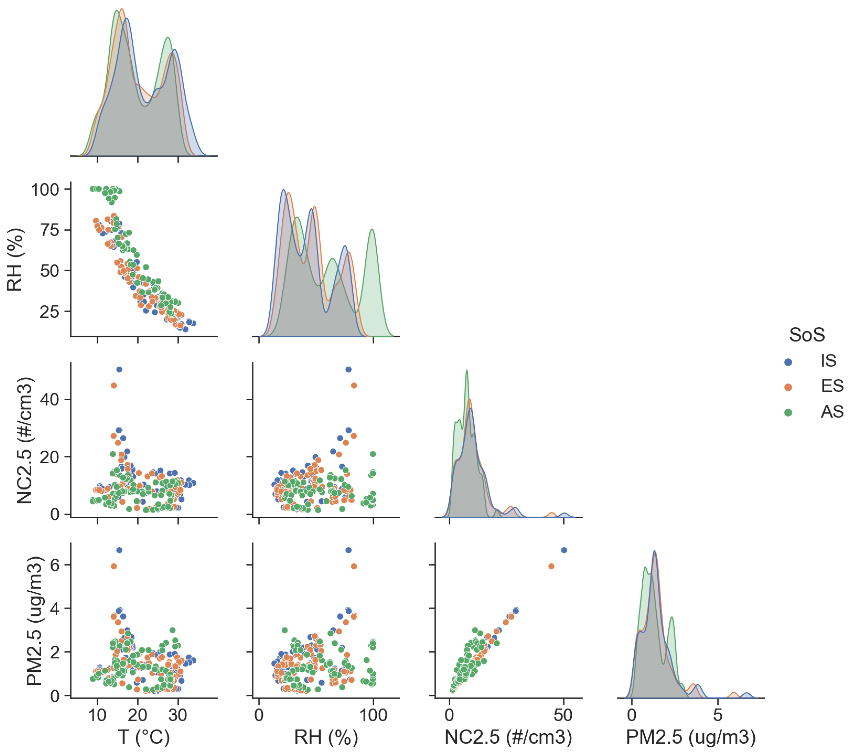
Figure 7.
Effect of RH on particle count with data aggregated in 4 RH bins.
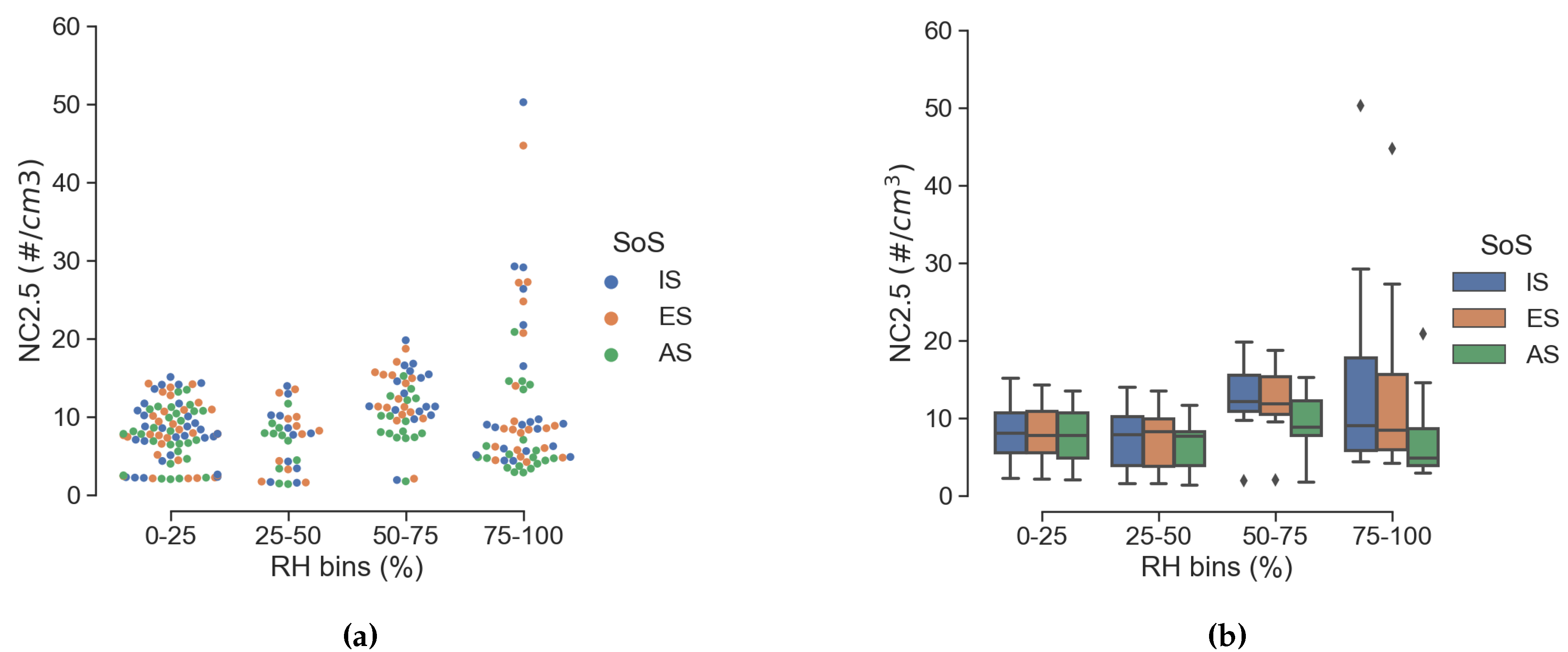
Figure 8.
Effect of RH on PM2.5 with data aggregated in 4 RH bins.
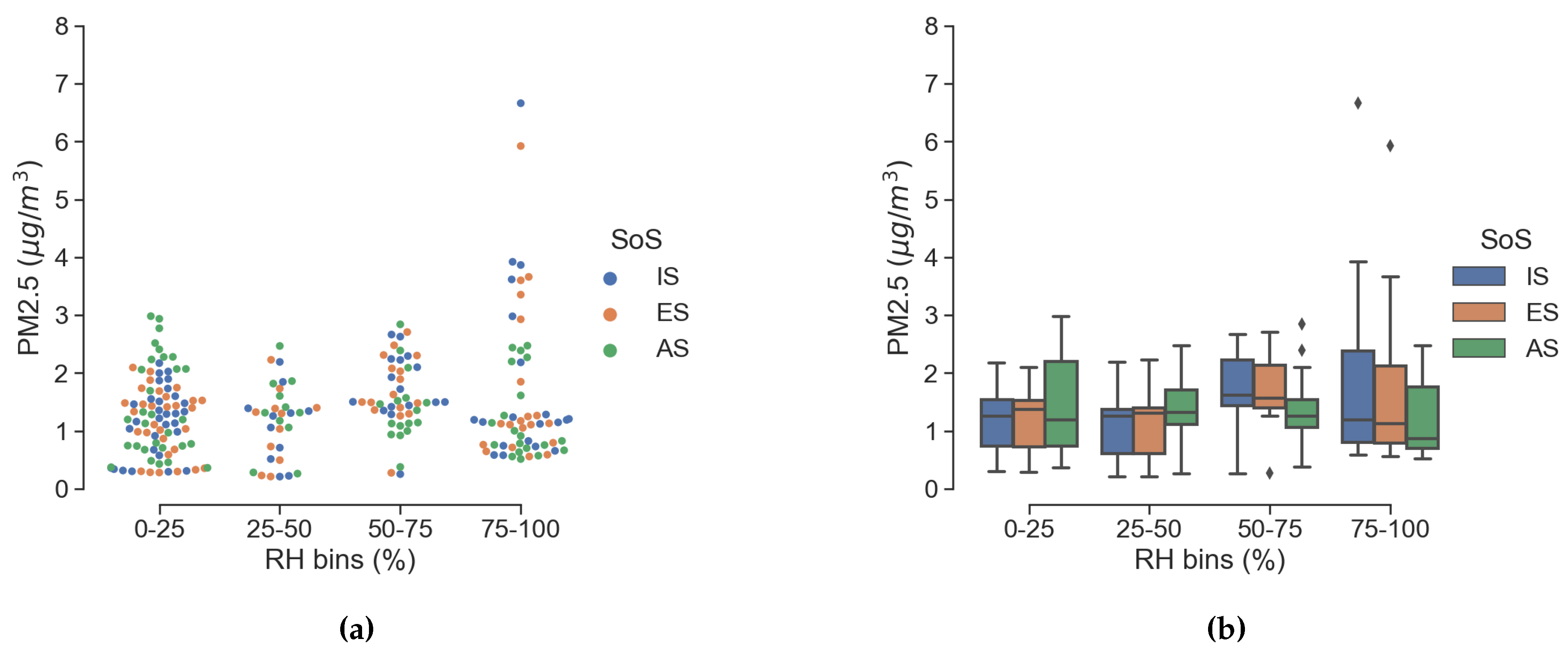
Figure 9.
Scatter plot of 2.5m particle count values without RH binning.
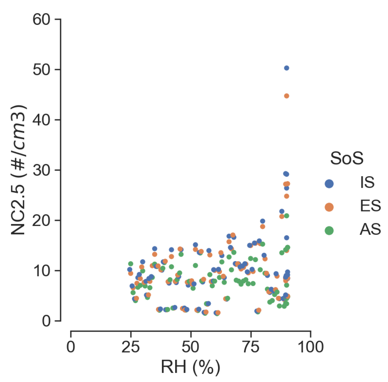
Figure 10.
Linear regression for particle size using the full data-set in terms of RH 0-100% or a reduced data-set with RH 0-50% (less data points).
Figure 10.
Linear regression for particle size using the full data-set in terms of RH 0-100% or a reduced data-set with RH 0-50% (less data points).
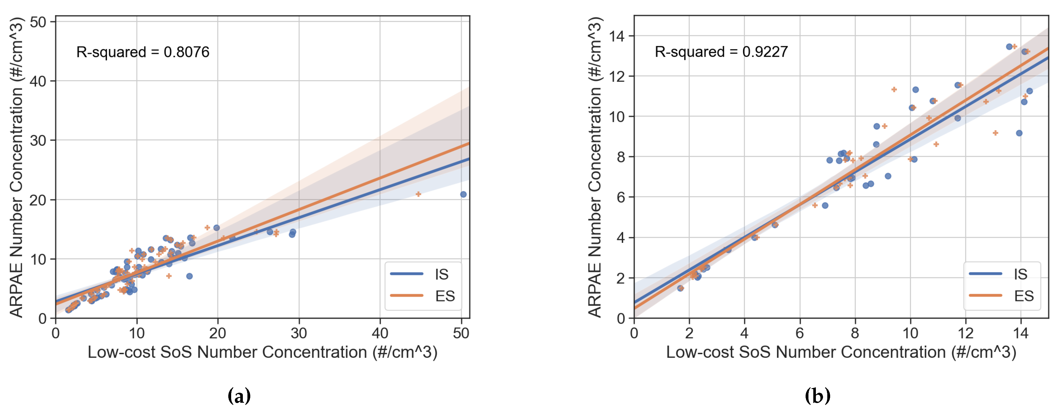
Figure 11.
Particle count to mass concentration conversion. (a) Calculated from particle count according to equation 1; (b) corrected according to reference station average particle mass.
Figure 11.
Particle count to mass concentration conversion. (a) Calculated from particle count according to equation 1; (b) corrected according to reference station average particle mass.
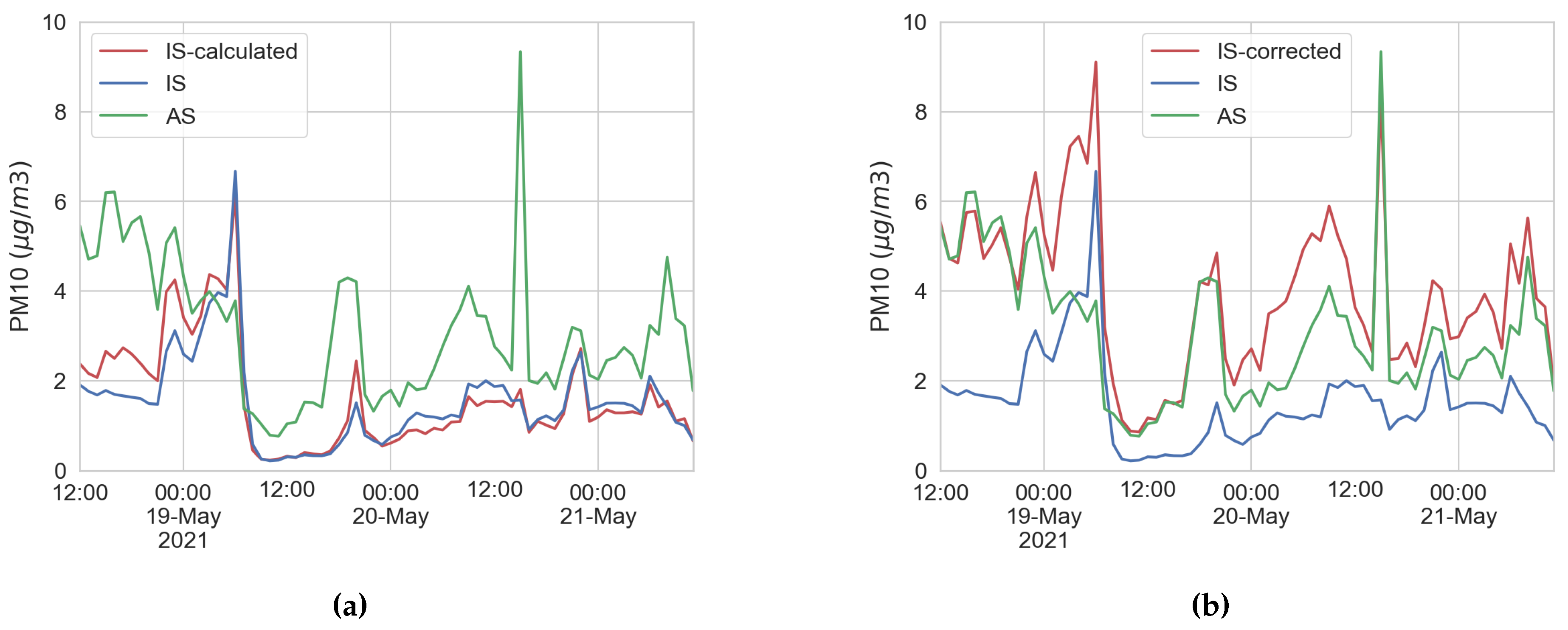

Table 1.
Measured quantities and daily summary.
| Variable | Specifications | Summary (Day2,Day3) | ||||
|---|---|---|---|---|---|---|
| (Unit) | Description | Sensor | IS | ES | AS | MSR |
| Air temp. | BME280 | (21.0,20.8) | (19.5,19.6) | (19.1,18.9) | (18.7,15.8) | |
| Air rel. hum. | BME280 | (51,43) | (55,46) | (71,62) | (42,57) | |
| PM1 conc. | SPS30 | (1,1) | (1,1) | (0,0) | n.d. | |
| PM2.5 conc. | SPS30 | (1.5,1.4) | (1.4,1.3) | (1.1,1.1) | (5.2,2.4) | |
| PM10 conc. | SPS30 | (2,1) | (1,1) | (2,3) | (15,6) | |
| Number conc. | SPS30 | (11,11) | (10,10) | (6,8) | n.d. | |
| Number conc. | SPS30 | (11,11) | (10,10) | (6,8) | n.d. | |
| Number conc. | SPS30 | (11,11) | (10,10) | (6,8) | n.d. | |
| a mv = measured value. | ||||||
Table 2.
Particle count buckets grouping.
| AS | IS, ES | ||
|---|---|---|---|
| Channel | size range ( ) | Channel | size range ( ) |
| 1 | 0.28-0.4 | 1 | 0.3-0.5 |
| 2 | 0.4-0.5 | ||
| 3 | 0.5-0.7 | 2 | 0.5-1.0 |
| 4 | 0.7-1.1 | ||
| 5 | 1.1-2.0 | 3 | 1.0-2.5 |
| 6 | 2.0-3.0 | ||
| 7 | 3.0-5.0 | 4 | 2.5-4 |
| 8 | 5.0-10 | 5 | 4.0-10 |
Disclaimer/Publisher’s Note: The statements, opinions and data contained in all publications are solely those of the individual author(s) and contributor(s) and not of MDPI and/or the editor(s). MDPI and/or the editor(s) disclaim responsibility for any injury to people or property resulting from any ideas, methods, instructions or products referred to in the content. |
© 2024 by the authors. Licensee MDPI, Basel, Switzerland. This article is an open access article distributed under the terms and conditions of the Creative Commons Attribution (CC BY) license (http://creativecommons.org/licenses/by/4.0/).
Copyright: This open access article is published under a Creative Commons CC BY 4.0 license, which permit the free download, distribution, and reuse, provided that the author and preprint are cited in any reuse.


