
Submitted:
09 July 2024
Posted:
10 July 2024
You are already at the latest version
Abstract
This paper presents a new algorithm to solve the optimal reconfiguration problem in distribution networks, using the algorithm called Improved Simulated Annealing combined with Hybrid Cooling (ISA-HC) and Selective Space Search, which leverages the capabilities of the Open Distribution System Simulator (OpenDSS) software and the selective space search concept to enhance performance and reduce the search space. The ISA-HC algorithm determines an adequate starting point for the temperature and initial solution according to the size of the system. For adequate cooling, a three-stage cooling approach was employed to achieve effective cooling, combining two methods widely used in the literature. Overall, the ISA-HC algorithm is a promising method for solving the optimal reconfiguration problem in distribution networks. The algorithm was tested on the systems of 5, 33, 69, and 94 buses and compared to other existing methods in the literature. The results show that the proposed method is more robust and efficient, providing better convergence and reliably achieving good-quality global solutions
Keywords:
distribution network reconfiguration
; improved simulated annealing
; selective space
; hybrid cooling
; optimization
1. Introduction
The Distribution System is a critical component that typically encompasses the final connections between power generation and end-users. The distribution systems use a radial design, which comprises a primary branch with subsidiary branches that extend throughout the system. This design is popular due to its simple structure, cost-effectiveness, and strong protection mechanisms. To ensure a continuous, efficient, reliable, and cost-effective electrical system, it is crucial to establish strategies and conduct studies that specifically address reliability improvement and loss minimization [1,2]. These aspects play a vital role in maintaining a stable and uninterrupted power supply while optimizing the overall performance of the system.
Distribution networks are prone to experiencing significant power losses, resulting in financial costs for companies that can only be mitigated rather than eliminated entirely. To minimize these technical losses, various strategies are commonly employed in the field. These include reconduction, voltage level increase, installation of capacitor banks, and network reconfiguration. Among these strategies, network reconfiguration stands out as a cost-effective approach as it utilizes existing network infrastructure, requiring minimal additional investment [3,4]. The traditional reconfiguration study seeks to find an optimal topology that generates the lowest possible losses in the system under study. The system topologies are generated by opening or closing the switches present in the system distribution. The reconfiguration problem does not involve the installation of new equipment or new power generation. The only costs of the reconfiguration are those associated with opening or closing switches, which are negligible [5].
The term “flexible and reconfigurable distribution network structure” has two interpretations. During normal network operation, it refers to minimizing losses, balancing the network load, and enhancing the network’s operational state. In the event of short circuits or power outages, grid reconfiguration refers to identifying viable configurations to ensure the greatest possible number of loads have access to electricity. The optimal solution for reconfiguration is one that results in the lowest network loss [6].
When modifying the network’s topology, several outcomes can emerge, including (i) the feeder load, (ii) energy losses, (iii) voltage levels, and (iv) reliability. The integration of distributed generation (DG) sources, such as wind and photovoltaic, along with the introduction of electric cars, has been reshaping the distribution network structure. The proliferation of these sources has a significant impact on energy flow and voltage profiles, elevating the importance of network reconfigurations, and necessitating more rapid adaptations to loads and DG, which have a dynamic behaviour over a day [7,8,9,10,11].
The task of identifying the optimal solution is known as combinatorial optimization. It is a challenging problem because there are numerous possible configurations in a distribution network, and this number increases as the network size expands. As a result, testing every potential configuration incurs a substantial computational cost. Considering that each switch can have two states, the number of possible configurations is , where n is the total number of switches in the system [12,13]. This way, deterministic approaches become practically unfeasible [14]. Therefore, there is a need to use computational algorithms and tools that substantially reduce the number of solutions to be tested and find a possible optimal or close-to-optimal solution with a substantially reduced and affordable computational cost.
In specialized literature, various approaches are explored for distribution network reconfiguration. We opt for intelligent algorithms due to their ability to handle the complexity of variable data. Unlike static solvers, such as simulated annealing, genetic algorithms, particle swarm optimization (PSO), and neural networks stand out for their adaptability and continuous learning, which are crucial for addressing the complex and nonlinear nature of these problems.
In this section, it will undertake a thorough examination of simulated annealing. Our analysis will concentrate on pinpointing specific deficiencies within the current applications of this metaheuristic strategy, where there is a substantial potential for enhancement. This investigation will be directed towards identifying and addressing these gaps, aiming to refine and elevate the efficacy of simulated annealing in complex optimization scenarios.
In a study conducted in 2008 described in [15], the authors used the simulated annealing algorithm to address the distribution network reconfiguration problem while incorporating load constraints into the objective optimization function. Similarly, in [16], simulated annealing was employed to improve network reliability by minimizing the cost associated with power supply interruptions to customers while also considering the operational limitations of the system. However, both simulated annealing methods had a high computational time consumption and no clear criterion was established for determining the initial temperature that fits the size of the network.
In [17], the Simulated Immune Annealing (SAI) algorithm is used to address the distribution network reconfiguration problem. This method utilizes shared switches between meshes to generate potential solutions and also leverages historical and current data to optimize the search. The proposed initial temperature adjustment, based on the relative behavior of the population, has been shown to yield satisfactory results. However, its dependency on the number of individuals can increase simulation time, which is an aspect that deserves optimization.
In a 2017 publication described in [18], the authors discussed the use of Simulated Annealing along with the Ant Colony algorithm to optimize the distribution network reconfiguration problem. They developed an algorithm called the Improved Hybrid Ant Colony Algorithm, which proved to be efficient in identifying the optimal solution. However, the hybrid method used had high computational consumption and only employed simulated annealing for the generation of individual pheromones.
In 2018, a study [12] compared simulated annealing with tabu search for network reconfiguration problems. Simulated annealing accepted suboptimal solutions to avoid local optima, while tabu search avoided repeated solutions. In systems with 16 and 33 buses, simulated annealing showed high computational efficiency but limitations in thoroughly reviewing solutions. Another study [19] proposed enhancing simulated annealing through incremental and random sequential changes in the network. Both studies noted that simulated annealing had high performance but lacked the ability to thoroughly review solutions and lacked a clear definition for the initial temperature.
In 2021, the simulated annealing method was applied in a study referenced as [20] to optimize the configuration of a distribution network over a full day. This study explored various optimization variables and used simulated annealing to find the most efficient network configuration. Additionally, during the same year, Nguyen et al. [21] proposed an enhancement to the cuckoo search method, adapting it from a continuous to a binary approach and introducing a new search mechanism. This evolution in methods facilitates obtaining higher-quality solutions in fewer iterations, highlighting the importance of integrating continuous improvements to achieve optimal results.
In 2022, in their thesis [22], the use of the simulated annealing algorithm was proposed for distribution systems using OpenDSS version 9.4.0.3 software. The study introduced the concept of Bus Generation, generating neighbors from the route from each bus to the slack bus. Although this improved the algorithm’s effectiveness, challenges were still encountered in terms of computational time and optimizing the initial temperature value determination.
Finally, in 2023, an approach to the distribution network reconfiguration (DNR) problem was presented in [23], which incorporates simultaneous switching of capacitors. The study combined the simulated annealing algorithm with the minimum spanning tree algorithm, achieving satisfactory performance while meeting technical, voltage, and capacity constraints. These improvements in traditional methods are crucial for providing effective solutions during the optimization phases.
When facing the complex task of reconfiguring networks in distribution systems, metaheuristic techniques are prominent solutions. Although simulated annealing is less frequently used, its effectiveness in addressing various challenges within the electrical sector has been demonstrated [24,25,26,27,28]. With appropriate improvements, this metaheuristic has the potential to offer even more efficient results for solving network reconfiguration problems. In this article, we refine the classic simulated annealing algorithm (SA), focusing on critical aspects such as computation time, selecting an initial temperature adapted to the network size without increasing simulation time, and a cooling model that facilitates a more effective search for solutions. We also address identified deficiencies and make improvements based on previous literature reviews. Furthermore, we have worked on strengthening its competitiveness against other widely used methods. We introduce the Improved Simulated Annealing with Hybrid Cooling (ISA-HC) algorithm, an innovative approach rigorously evaluated on four widely recognized distribution systems in the literature. The main contributions of this article are succinctly summarized in the following points:
- (a)
- Selective Space Mesh Utilization: The introduction of a selective space mesh for generating neighbors focuses on key configurations of the problem, effectively reducing the search space. This strategy optimizes exploration by restricting it to specific neighborhoods with high potential for improvement.
- (b)
- Improved Initial Temperature Equation: Improving the initial temperature equation involves considering the average losses of “n” initial solutions, which effectively tailors the algorithm to the network size. This approach allows fine-tuning of the temperature initialization process by leveraging collective insights gained from multiple initial solutions.
- (c)
- Incorporation of Hybrid Cooling and Stopping Criteria: Incorporating stopping criteria and hybrid cooling methods improves solution acceptance and reduces iteration requirements. This dynamic combination of cooling strategies not only optimizes exploration of the search space but also enhances the algorithm’s effectiveness in finding high-quality solutions more efficiently.
- (d)
- Introduction of Cooling Rate Criteria: The proposal suggests advancing to the next temperature after accepting a specific number of neighbors, which enhances algorithm convergence and significantly reduces necessary computation time. This approach enables focusing computational efforts on promising regions within the search space.
- (e)
- Computational Efficiency and Reliable Solution Attainment: The study confirms that the ISA-HC algorithm not only demonstrates computational efficiency but also consistently ensures the attainment of high-quality global solutions.
Overall, this work presents significant advancements in the algorithm’s efficiency, convergence, and solution quality, making it a valuable contribution to the field of distribution network reconfiguration.
This paper is structured as follows: Section 2 introduces the mathematical formulation of the reconfiguration problem. Section 3 explores the classical Simulated Annealing (SA) algorithm. The proposed method, Improved Simulated Annealing with Hill Climbing (ISA-HC), is detailed in Section 4, followed by its application to the reconfiguration problem in Section 5. Section 6 discusses the results obtained from the proposed method. Finally, Section 7 concludes the paper, summarizing key findings and implications.
2. Distribution Network Reconfiguration (DNR)
The reconfiguration of distribution networks is a multi-objective and non-linear optimization problem, with several objectives such as minimizing losses, improving reliability parameters, balancing transformer and feeder loads, maximizing feeder loads, and improving voltage profiles. To determine the switch states, the existing resources in the system are utilized [3].
In addition to minimizing losses, the reconfiguration problem also takes into account radiality constraints, voltage limits, branch current capacity, and the requirement to connect all loads in the system.
The fitness function, also known as the objective function, is defined by Equation (1):
Here, is the number of lines in the distribution network, is the resistance of line l, is the current flowing through line l, and represents the sum of all active losses in the lines. The system solution x corresponds to the configuration of switches.
The loss evaluation is obtained through the OpenDSS software, which uses a method that is detailed in [29,30,31].
2.1. Constraints
2.1.1. Voltage Constraints
The voltage level of the system buses must be within a certain range, which is specified by the following Equation (2):
Here, and are the minimum and maximum permissible values for the bus k, respectively.
2.1.2. Current Constraints
The current limits of the lines, determined by their technical characteristics, must also be taken into account. The current flowing through line l cannot exceed its maximum allowable capacity , as shown in Equation (3).
2.1.3. Radiality Constraints
The distribution network must maintain a radial topology, meaning that there should be only one path from any bus to its substation. This condition can be achieved with the help of the switches’ opening and closing states. The radial structure ensures that there are no loops in the network, and all loads are connected and energized by the substation fulfilling the Equations (4) and (5). The conditions for radiality are based on [32,33].
-
The number of meshes in the system when all switches are closed can be determined using the following formula:Here, is the number of meshes, is the total number of active lines, and is the total number of buses in the system.
-
The total number of lines in the system can be obtained by subtracting the number of sources from the total number of buses:Here, is the number of active lines, is the total number of buses, and is the number of sources.
- The entire system must be connected and energized, meaning that all loads are supplied by a substation or sources.
3. Classical Simulated Annealing Algorithm
The Simulated Annealing (SA) proposed by Kirkpatrick in 1983 , one of the many algorithms that emerged in natural computation, a science that uses natural systems as inspiration to solve computational problems. For the SA, the inspiration comes from the physical-chemical area, where they seek to imitate the annealing of materials such as metals or glass [34].
In [35] they mention that SA is inspired by the annealing process in metallurgy. In this natural process, a material is slowly heated and cooled under controlled conditions to increase the size of the crystals and reduce their defects. Improving the resistance and durability of the material.
3.1. Simulated Annealing Strategy
From [34], it is mentioned that SA bases its strategy on three characteristics:
- Use of a starting solution;
- Random generation of new solutions based on the current solution;
- Progressively elitist criterion to change the random solution for the current one.
3.2. Mathematical Representation and Parameters
The simulated annealing algorithm is characterized by its ability to escape from the local optimum, based on the acceptance rule of a candidate solution. If the objective function value of the new solution is smaller (assuming minimization) than the previous solution , then the new solution is accepted. Otherwise, the new solution can also be accepted if the value given by the Boltzmann distribution (6) is greater than a uniform random number between 0 and 1. Here, T is the control parameter known as “temperature” [36]. The objective function and parameters used in the algorithm are:
The Simulated Annealing method involves several key components:
- Objective function: This function defines the property that needs to be minimized or maximized depending on the application.
- Initial population: The iterative technique requires an initial guess for the parameter values.
- Initial temperature: The control parameter ’temperature’ is carefully defined, since it controls the rule defined in (6). Initial temperature: The ’temperature’ control parameter is critical as it governs the acceptance rule in Equation (6). The value of T should be high enough to allow escape from local minima but not too high to stray from a global minimum. An example of the initial temperature definition is shown in Equation (7) used in [22]:
- Perturbation mechanism: This method creates new solutions from the current solution.
- Cooling: The geometric rule is commonly used to reduce the temperature.
- Termination criteria: Various methods exist to control the completion of Simulated Annealing as mentioned in [36].
4. Proposed Method
The proposed method utilizes the OpenDSS software as a solution engine for processing power flow data, as well as data related to voltages, energies, currents, losses, and other related factors.
4.1. Initial Solution and Initial Temperature
The initial temperature, , plays a pivotal role in the Simulated Annealing (SA) process. Setting too high leads to a search that is essentially random, while a temperature set too low restricts the search to a local vicinity, thereby limiting exploration and reducing the chances of identifying high-quality solutions. To address this, we propose an adaptive equation for that scales according to the size of the network, ensuring efficient exploration without unduly extending the simulation time. This method balances the breadth and depth of the search space exploration, optimizing the algorithm’s performance across various network configurations.
The initial temperature is determined using the variable parameter “C” and the number of initial solutions. This approach enhances the Equation (7) proposed by [22].
The variable “LossAverage” represents the average losses of “n” initial solutions (IniSol), while “C” is a constant that takes on values within the range of [0,1].
Equations (8) and (9) allow us to obtain a suitable temperature based on the size of the system. The initial solution, which has the minimum losses among the “n” initial solutions, is determined using Equation (10).
Here, refers to the solution that will be utilized as the initial configuration, and its losses will serve as the starting losses for the algorithm. , , …, represent the “n” initial solutions generated.
4.2. Selective Space Mesh (SSM)
In the Selective Space Mesh (SSM) approach, each line in the system is equipped with a single switch that can be operated. Therefore, the number of operable switches (nc) is equal to the number of lines (nl). For instance, in a system comprising 5 buses and 7 lines, there can be = 128 possible configurations.
Equation (4) enables us to obtain 3 meshes. As per the approach proposed by [3] and [2], each switch belongs to only one mesh. For instance, in the case of a 5-bus system, mesh 1 comprises lines [1, 2, 3], mesh 2 consists of lines [4, 5], and mesh 3 includes lines [6, 7] (refer to Figure 1). Therefore, the number of possible configurations can be obtained by multiplying the number of switches in each mesh. For this system, there are 3 × 2 × 2 = 12 possible configurations, which is a relatively small number.
4.3. Cooling Mechanisms
Several cooling mechanisms are used in the literature. In this article, we have employed the geometric cooling model, where the temperature reduction is defined by , with varying between 0.8 and 0.99. For example, a value of results in faster cooling than . Additionally, we consider the model proposed by Lundy and Mees [37], which controls the number of iterations until reaching the final temperature. The geometric scheme promotes greater diversification in the search at higher temperatures, while the Lundy-Mees method is more suitable for lower temperatures. This contrast is illustrated in Figure 2, adapted from [37].
The hybrid cooling mechanism proposed in this article is called GDLM (Geometric Double Lundy and Mees). As illustrated in Figure 3, GDLM employs a fast geometric () cooling mechanism followed by a slower one (), and finally, the Lundy and Mees scheme is applied to achieve a reheat and cool to the final temperature. The conditions that define this mechanism are presented in Equation (11):
The model accelerates initial cooling using during the first 30% of the total temperature range. Then, between 30% and 80%, we increase to 0.95 for a more gradual cooling. Finally, in the last 20% of the temperature range, we apply the Lundy & Mees method to adjust the final temperature through a controlled process of heating and cooling.
Equations for Lundy & Mees:
where:
represents the reheat factor, which is the temperature at which the Lundy and Mees cooling mechanism begins. M denotes the total number of iterations, k is the current iteration number, and is the multiplier of the number of iterations. In this study, we have used , which is three times the number of iterations used for geometric cooling.
If we take , this means that the initial temperature for the Lundy and Mees method will be 75% of the initial temperature (). Additionally, M represents the total number of iterations we desire from to . The calculation of M depends on and the iteration k we are in. For example, if the geometric cooling ends at iteration k = 150, and we choose = 3, we are indicating a total of 450 iterations, of which 150 are for geometric cooling and 300 correspond to the Lundy and Mees method.
4.4. Cooling Rate
The cooling rate is represented by , which is the duration that the algorithm spends at a specific temperature. This duration can either be fixed or can be determined based on an equilibrium condition. In this study, we adopt a different approach, which involves cooling the system when the maximum number of neighbors has been generated () or when a maximum number of neighbors has been accepted (). It should be noted that must be greater than , and the following condition (16) is applied to ensure this:
where: is a constant that takes values between 0 and 0.6, indicating the proportion of the maximum number of neighbors that are accepted as successful solutions. A good choice for this constant is .
If we have a maximum number of neighbors (NNm) equal to 25 and , the transition to the next temperature will occur when either 25 neighbors have been generated or when the neighbors accepted according to the acceptance criterion are round (0.1 × 25) = 3.
4.5. Acceptance Criterion
In each iteration at temperature , several neighbors are generated, and each one is evaluated using a dual acceptance criterion: if it improves the current solution, it is automatically updated; otherwise, a probability is calculated using the Boltzmann equation. We generate a random number between 0 and 1, and if it is less than the calculated value, the neighboring solution replaces the current solution. This strategy allows the Simulated Annealing algorithm to avoid local optima and effectively explore alternative solutions. The algorithm uses the acceptance function defined by Equation (18).
where: , neighbor solution, s is the current solution, is a random number between [0,1] and is the Objective Function.
4.6. Stopping Criteria
In principle, the temperature that represents the coldest possible state is zero (). However, before reaching this value, the probability of accepting a worse solution, as determined by the expression , becomes negligible.
Two criteria are proposed. The first criterion is met when the temperature is less than or equal to the final temperature, set at 0.01 for this study. The second criterion is achieved when, after a defined number of iterations (nFO), the temperature state repeatedly converges to the best solution found up to that moment (19).
The chosen combination of stop criteria and cooling conditions ensures a balance in the search process, preventing unnecessary resource consumption.
4.7. Neighbor Generator
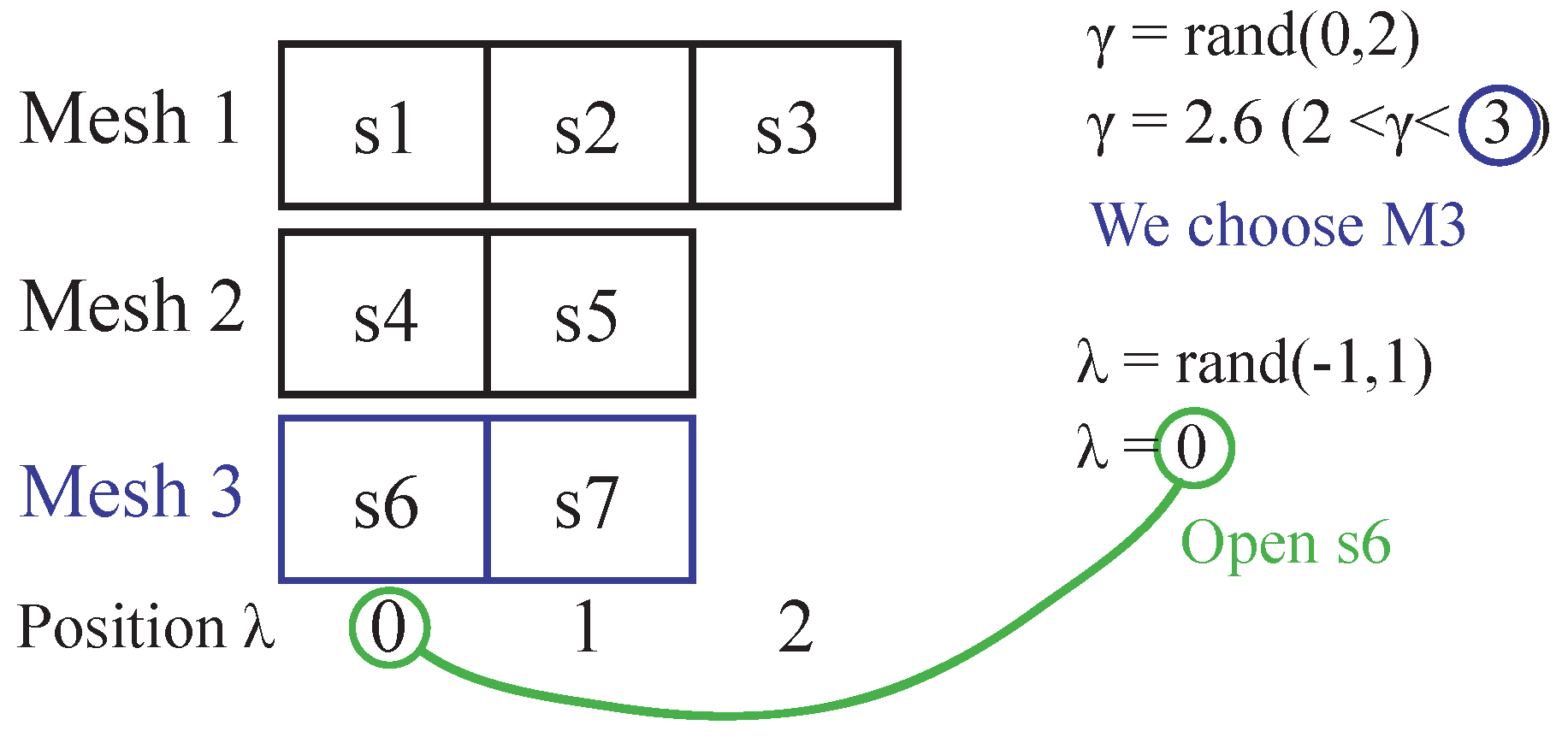
The neighbor generator is a crucial component of the simulated annealing algorithm, as it is responsible for generating candidate solutions for the optimization problem. In this study, the dimension of the system is determined using the SSM. Then, uniform random neighbors are generated that take values in the range of [0, ], where is the number of SSM. This neighbor generation process allows for the exploration of the solution space in a systematic and controlled way. A mesh is taken according (20):
From the chosen “” mesh, the position of the switch that must open is given by (21), the first position being the value of 0:
where: number of mesh switches, uniform random integer.
Considering the 5-bus system with 3 defined meshes: M1 = [1,2,3], M2 = [4,5] and M3 = [6,7]. To generate the first neighbor, a random number is chosen in the range from 0 to 2 (since there are 3 possible meshes). If turns out to be 2.6 (within the range 2 to 3), mesh M3 is selected. To determine which switch in this mesh to open, another random integer is generated in the range from −1 to 1, given that the mesh has two switches. If is 0, the first switch s6 is opened. If is −1, the absolute value (1) indicates opening the second switch, s7. This process is repeated to generate the other neighbors.
Figure 4.
Neighbor Generator Steps.
5. Application of the ISA-HC in DNR
The ISA-HC algorithm follows the following steps:
- Declare input data, network configuration, constants, and parameters.
- Define search spaces dimensions.
- If the temperature is greater than the Tf and the number of repetitions of the best solution found is less than the maximum number of repetitions, continue with step 5, otherwise go to step 12.
- If the number of successes is less than Equation (16) and the generated neighbors are less than the maximum number allowed, go to step 6, otherwise go to step 10.
- Generate a random nearest neighbor using the method described in the proposed methodology, calculate the fitness function for the generated neighbor by running a load flow analysis using OpenDSS.
- If the candidate solution improves the losses, it is updated as the best solution and the repetition count is restarted.
- The neighbor counter increases by one and return to step 5.
- If the candidate solution matches the best solution, the number of repetitions increases by one. Go to step 11
- Apply hybrid temperature cooling using Equation (11) and proceed to step 4.
- Displays the results.
The complete flowchart of the algorithm is shown in Figure 5.
6. Simulation and Results
The DNR problems for the distribution systems of 5, 33, 69, and 94 buses, which are widely used in the technical literature, were solved using the ISA-HC method. An Intel(R) Core(TM) i5-7200U CPU @ 2.50 GHz 2.70 GHz laptop was used. The required parameters for these systems were C, number of initial solutions, , and . The other parameters were kept constant, with values of = 0.9, = 0.95, = 3, = 0.95, and = 0.01.
6.1. Case Study 1
In this case study, we will examine the didactic 5-Bus system with 7-Line that was extracted from [38]. The system comprises a substation located at Bus 1, 4 sectionalizing switches (s1, s3, s5, and s7), and 3 tie switches (s2, s4, and s6). Figure 1 depicts the generated meshes. The Table 1 shows the results for different values of the parameters n, NNm and . Keeping the parameter C constant.
The following parameters were set for the system: maximum number of neighbors generated = 5, the simulation will end before reaching when = 20 iterations of the best current FO is achieved, C = 0.1 to 0.9, since it is a small system, only 2 initial solutions are considered.
Based on Table 2, it can be observed that only 2 initial solutions with a value of are sufficient. The literature reports as the best solution found [3, 4, 7] for this system, which was also used for testing the algorithm. In the Figure 6 a comparison is made with SA methods, where there is a better beginning of To, therefore with losses very close to the final solution. The legend displays the number of iterations required to achieve convergence for each method. It is possible to reach the solution with the same number of iterations as Andrade who uses a fast cooling value of 0.7. ISA-HC on average takes 0.51 s, Amorim 3.1 s, Andrade (C = 0.1) 0.85 s and for (C = 0.8) 0.96 s.
Table 3 provides a comparison of the proposed method with other existing methods found in the literature, showcasing the favorable results obtained by the proposed approach. The table likely presents various performance metrics or evaluation criteria used to assess the effectiveness of different methods in solving a particular problem.
6.2. Case Study 2
The 33-Bus 10 MVA system, proposed by Baran and Wu [3,40], is a 5-dimensional distribution system operating at 12.66 kV, with 37 branches, 32 sectionalizing switches, and 5 tie switches. The generated meshes for this system are illustrated in Figure 7. The Table 4 shows the results for different values of the parameters n, NNm and . Keeping the parameter C constant.
The following parameters were employed in the ISA-HC method: the maximum number of neighbors generated = 20, the simulation will end before reaching when = 20 iterations of the best current FO is achieved, C = 0.1 to 0.9, since it is a small system, 2 initial solutions are considered.
Table 5 demonstrates that for the 33-bus system, the proposed method achieved favorable results using only 2 initial solutions and a value of . The literature reports that the best solution found for this system is [7, 9, 37, 14, 32]. The proposed method, according to the information provided, also reached the same solution. This indicates that the proposed method is effective in finding the best solution for the 33-bus system, matching or even surpassing the results reported in the literature. It showcases the competitiveness and capability of the proposed method in solving complex optimization problems in the context of the 33-bus system.
Table 6 presents a comparison of the proposed method with other methods documented in the literature, highlighting the positive outcomes achieved by the proposed approach. The table includes evaluation criteria used to assess the effectiveness of various methods in solving the specific problem related to the 33-bus system. The Figure 8 shows that the proposed method starts with a better initial solution than the other methods and with a smaller number of iterations (55). The legend displays the number of iterations required to achieve convergence for each method. ISA-HC on average takes 4.25 s, Amorim 19.87 s, Andrade (C = 0.1) 12.9 s and for (C = 0.8) 23.35 s.
6.3. Case Study 3
The 69-Bus system with 10 MVA, originally presented in [43], with data taken from Savier and Das [44], is a five-dimensional system that consists of 73 branches, 68 sectionalizing switches, and 5 tie switches, all fed by a 12.66 kV substation. Figure 9 illustrates the generated meshes for this system. The Table 7 shows the results for different values of the parameters n, NNm and . Keeping the parameter C constant.
The following parameters were used: the maximum number of neighbors generated = 25, the simulation will end before reaching when = 20 iterations of the best current FO is achieved, C = 0.1 to 0.9, since it is a medium system, 4 initial solutions are considered.
Based on the information provided, Table 8 indicates that for the 69-bus system, the proposed method yielded promising results using only 4 initial solutions and setting . Comparing with the literature, it is reported that the best solution found for this system is [69, 14, 70, 55, 61]. Notably, the proposed method also achieved the same solution, demonstrating its effectiveness in obtaining the optimal solution for the 69-bus system.
Table 9 presents a comparative analysis of the proposed method with other methods documented in the literature, indicating the favorable results obtained by the proposed approach. The Figure 10 shows that the proposed method starts with a better initial solution than the other methods and with a smaller number of iterations (75). The legend displays the number of iterations required to achieve convergence for each method. ISA-HC on average takes 13.74 s, Amorim 33.24 s, Andrade (C = 0.1) 26.95 s and for (C = 0.8) 25.9 s.
6.4. Case Study 4
The 94-bus system with 100 MVA of Su and Lee [45] is a real distribution system belonging to Taiwan Power Company (TPC). The system consists of eleven feeders, composed of 96 branches, 83 sectionalizing switches, and 13 tie switches, all fed by an 11.4 kV substation. The system has a dimension of 13. Figure 11 displays the generated meshes. The Table 10 shows the results for different values of the parameters n, NNm and . Keeping the parameter C constant.
For this system, the parameters were set as follows: the maximum number of neighbors generated = 35, the simulation will end before reaching when = 30 iterations of the best current FO is achieved, C = 0.1 to 0.9, for this large system, the number of initial solutions will be 6.
According to Table 11, only 6 initial solutions with a value of are sufficient. The literature reports that the best solution found [55, 7, 86, 72, 13, 89, 90, 83, 92, 39, 34, 42, 62] for this system, the proposed method achieves the same reported solution with a standard deviation of zero.
Table 12, provides a comparative analysis of the proposed method with other methods documented in the literature, demonstrating the favorable results achieved by the proposed approach.
The Figure 12 shows that the proposed method starts with a better initial solution than the other methods and with a smaller number of iterations (80). The legend displays the number of iterations required to achieve convergence for each method. ISA-HC on average takes 20.26 s, Amorim 56.88 s, Andrade (C = 0.1) 39.8 s and for (C = 0.8) 47.55 s.
7. Conclusions
This paper introduces the Improved Simulated Annealing with Hybrid Cooling (ISA-HC) method, featuring a novel three-phase cooling strategy. The first two phases incorporate the geometric method with variable alpha, enabling both rapid and gradual temperature changes for effective exploration of the solution space. The third phase integrates the Lundy & Mees method, specifically tailored for low temperatures, ensuring efficient cooling and enhancing solution acceptance through the Boltzmann equation.
The implementation of the Selective Space Mesh in all four systems contributes to improved neighbor generation, focusing on relevant configurations and enhancing the search for candidate solutions. Addressing the challenge of defining the initial temperature in Simulated Annealing, ISA-HC provides an equation adapted to the system size, mitigating its impact on the final solution. This improvement is evident in the method comparison graphs, particularly during iteration 0 in the analyzed systems.
By meticulously controlling the cooling process and incorporating appropriate stopping criteria, ISA-HC avoids unnecessary computational resource expenditure. This optimization strategy results in faster simulations, quicker convergence, and more efficient solution exploration. The cooling rate plays a crucial role in reducing calculation time during neighbor generation, ensuring the acquisition of only essential neighbors for a given temperature.
The proposed method encompasses various contributions, each directly or indirectly reducing convergence time and positively influencing solution quality and computational efficiency. ISA-HC achieves a 40% to 70% reduction in the number of iterations and computation times compared to other methods, establishing its competitiveness among metaheuristics. The comparative tables from 100 simulations demonstrate the method’s high attractiveness and efficiency, consistently achieving the reported solution with 100% effectiveness. The results suggest that, for the initial temperature equation, it is advisable to use values between [0.1–0.3] for the parameter C.
One limitation of the proposed approach is its applicability to distribution systems with distributed generation, such as photovoltaic plants. Future work will evaluate how the integration of photovoltaic generation affects system optimization and will investigate the proposed method, as well as a combination of the ISA-HC method with other metaheuristics, to improve efficiency and robustness in more complex energy distribution scenarios.
Author Contributions
Conceptualization, C.C.C. and F.J.S.P.; Investigation, F.J.S.P., Methodology, F.J.S.P. and Y.P.M.R.; Software, F.J.S.P. and Y.P.M.R, Validation, F.J.S.P., C.C.C., Y.P.M.R. and D.Z.Ñ.H.; Funding Acquisition, C.C.C.; Resources, C.C.C., Writing—Original Draft Preparation, F.J.S.P.; Writing—Review and Editing, F.J.S.P., Y.P.M.R. and D.Z.Ñ.H. All authors have read and agreed to the published version of the manuscript.
Funding
This research was funded by UNI (Universidad Nacional de Ingeniería).
Data Availability Statement
Dataset available on request from the authors.
Conflicts of Interest
The authors declare no conflict of interest.
References
- Pegado, R.D.A. Reconfiguração de Redes de Distribuição de Energia eléTrica Usando Otimização por Enxame de partíCulas Aprimorado. Master’s Thesis, Universidade Federal da Paraíba, João Pessoa, Brazil, 2019. [Google Scholar]
- Pinheiro Filho, L.O. Reconfiguração de Redes de Distribuição Utilizando Algoritmo de Busca Tabu. Master’s Thesis, Universidade Federal da Paraíba, João Pessoa, Brazil, 2022. [Google Scholar]
- Pegado, R.; Ñaupari, Z.; Molina, Y.; Castillo, C. Radial distribution network reconfiguration for power losses reduction based on improved selective BPSO. Electr. Power Syst. Res. 2019, 169, 206–213. [Google Scholar] [CrossRef]
- Anteneh, D.; Khan, B.; Mahela, O.P.; Alhelou, H.H.; Guerrero, J.M. Distribution network reliability enhancement and power loss reduction by optimal network reconfiguration. Comput. Electr. Eng. 2021, 96, 107518. [Google Scholar] [CrossRef]
- Dias Santos, J.; Marques, F.; Garcés Negrete, L.P.; Andrêa Brigatto, G.A.; López-Lezama, J.M.; Muñoz-Galeano, N. A Novel Solution Method for the Distribution Network Reconfiguration Problem Based on a Search Mechanism Enhancement of the Improved Harmony Search Algorithm. Energies 2022, 15, 2083. [Google Scholar] [CrossRef]
- Nie, S.; Fu, X.P.; Li, P.; Gao, F.; Ding, C.D.; Yu, H.; Wang, C.S. Analysis of the impact of DG on distribution network reconfiguration using OpenDSS. In Proceedings of the IEEE PES Innovative Smart Grid Technologies, Berlin, Germany, 14–17 October 2012; pp. 1–5. [Google Scholar] [CrossRef]
- Marques, R.C.; Eichkoff, H.S.; de Mello, A.P.C. Analysis of the distribution network reconfiguration using the OpenDSS® software. In Proceedings of the 2018 Simposio Brasileiro de Sistemas Eletricos (SBSE), Niteroi Brazil, 12–16 May 2018; pp. 1–6. [Google Scholar] [CrossRef]
- Mello, A.P.C.d. Reconfiguração de Redes de Distribuição Considerando multivariáVeis e Geração Distribuída. Master’s Thesis, Universidade Federal de Santa Maria, Santa Maria, Brazil, 2014. [Google Scholar]
- Bernardon, D.P. Novos Métodos para Reconfiguração das Redes de Distribuição a partir de Algoritmos de Tomadas de Decisão Multicritérios. Ph.D. Thesis, Universidade Federal de Santa Maria, Santa Maria, Brazil, 2007; p. 229. [Google Scholar]
- Antončič, M.; Mikec, M.; Blažič, B. Development of distribution network model in OpenDSS using MATLAB and GIS data. In Proceedings of the 2019 7th International Youth Conference on Energy (IYCE), Bled, Slovenia, 3–6 July 2019; pp. 1–6. [Google Scholar] [CrossRef]
- Zeb, M.Z.; Imran, K.; Khattak, A.; Janjua, A.K.; Pal, A.; Nadeem, M.; Zhang, J.; Khan, S. Optimal Placement of Electric Vehicle Charging Stations in the Active Distribution Network. IEEE Access 2020, 8, 68124–68134. [Google Scholar] [CrossRef]
- De Andrade, B.A.R.; Ferreira, N.R. Simulated annealing and tabu search applied on network reconfiguration in distribution systems. In Proceedings of the 2018 Simposio Brasileiro de Sistemas Eletricos (SBSE), Niteroi, Brazil, 12–16 May 2018; pp. 1–6. [Google Scholar] [CrossRef]
- Chiang, H.D.; Jean-Jumeau, R. Optimal network reconfigurations in distribution systems. I. A new formulation and a solution methodology. IEEE Trans. Power Deliv. 1990, 5, 1902–1909. [Google Scholar] [CrossRef]
- Gerez, C.; Coelho Marques Costa, E.; Sguarezi Filho, A.J. Distribution Network Reconfiguration Considering Voltage and Current Unbalance Indexes and Variable Demand Solved through a Selective Bio-Inspired Metaheuristic. Energies 2022, 15, 1686. [Google Scholar] [CrossRef]
- Zhigang, M. Study on distribution network reconfiguration based on genetic simulated annealing algorithm. In Proceedings of the 2008 China International Conference on Electricity Distribution, Guangzhou, China, 10–13 December 2008; pp. 1–7. [Google Scholar] [CrossRef]
- Skoonpong, A.; Sirisumrannukul, S. Network Reconfiguration for Reliability Worth Enhancement in Distribution Systems by Simulated Annealing. In Proceedings of the 2008 5th International Conference on Electrical Engineering/Electronics, Computer, Telecommunications and Information Technology, Krabi, Thailand, 14–17 May 2008; Volume 2, pp. 937–940. [Google Scholar] [CrossRef]
- Chen, J.; Zhang, F.; Zhang, Y. Distribution Network Reconfiguration Based on Simulated Annealing Immune Algorithm. Energy Procedia 2011, 12, 271–277. [Google Scholar] [CrossRef]
- Chen, E.K.; Zhang, S.; Wang, T. Research on distribution network reconstruction based on improved simulated annealing—Ant colony algorithm. In Proceedings of the 2017 Chinese Automation Congress (CAC), Jinan, China, 20–22 October 2017; pp. 3575–3579. [Google Scholar] [CrossRef]
- Koziel, S.; Rojas, A.L.; Moskwa, S. Power loss reduction through distribution network reconfiguration using feasibility-preserving simulated annealing. In Proceedings of the 2018 19th International Scientific Conference on Electric Power Engineering (EPE), Brno, Czech Republic, 16–18 May 2018; pp. 1–5. [Google Scholar] [CrossRef]
- Zhang, J.; Li, Z.; Wang, B. Within-day rolling optimal scheduling problem for active distribution networks by multi-objective evolutionary algorithm based on decomposition integrating with thought of simulated annealing. Energy 2021, 223, 120027. [Google Scholar] [CrossRef]
- Nguyen, T.T.; Nguyen, T.T.; Le, B. Optimization of electric distribution network configuration for power loss reduction based on enhanced binary cuckoo search algorithm. Comput. Electr. Eng. 2021, 90, 106893. [Google Scholar] [CrossRef]
- Amorim, J.R.B.d.C. Reconfiguração da Rede de Distribuição Inteligente Usando Recozimento Simulado. Master’s Thesis, Universidade Federal da Paraíba, João Pessoa, Brazil, 2022. [Google Scholar]
- Stojanović, B.; Rajić, T.; Šošić, D. Distribution network reconfiguration and reactive power compensation using a hybrid Simulated Annealing—Minimum spanning tree algorithm. Int. J. Electr. Power Energy Syst. 2023, 147, 108829. [Google Scholar] [CrossRef]
- Tomczyk, M.; Mielnik, R.; Plichta, A.; Goldasz, I.; Sułowicz, M. Identification of Inter-Turn Short-Circuits in Induction Motor Stator Winding Using Simulated Annealing. Energies 2021, 15, 117. [Google Scholar] [CrossRef]
- Wu, M.; Chen, W.; Tian, X. Optimal energy consumption path planning for quadrotor UAV transmission tower inspection based on simulated annealing algorithm. Energies 2022, 15, 8036. [Google Scholar] [CrossRef]
- Tabak, A.; İlhan, İ. An effective method based on simulated annealing for automatic generation control of power systems. Appl. Soft Comput. 2022, 126, 109277. [Google Scholar] [CrossRef]
- Mohammad, K.; Basu, S.; Prasad, T.N.; Muthu, R.; Naidu, R.C. Optimizing Hydrogen Consumption in Fuel cells Using Simulated Annealing Algorithm. In Proceedings of the 2022 7th International Conference on Environment Friendly Energies and Applications (EFEA), Bagatelle Moka MU, Mauritius, 14–16 December 2022; pp. 1–5. [Google Scholar]
- Kida, A.A.; Rivas, A.E.L.; Gallego, L.A. An improved simulated annealing—Linear programming hybrid algorithm applied to the optimal coordination of directional overcurrent relays. Electr. Power Syst. Res. 2020, 181, 106197. [Google Scholar] [CrossRef]
- Sexauver, J. New User Primer: The Open Distribution System Simulator (OpenDSS). Train. Mater 2012, 7.6, 1–35. [Google Scholar]
- Montenegro, D. Introduction to the Next Generation of Distribution Analysis Tools—Summer course D1. In Proceedings of the 2019 IEEE Workshop on Power Electronics and Power Quality Applications (PEPQA), Manizales, Colombia, 30–31 May 2019; pp. 1–105. [Google Scholar]
- Dugan, R.C.; Montenegro, D. Reference Guide: The Open Distribution System Simulator (OpenDSS); Electric Power Research Institute, Inc: Washington, DC, USA, 2020; Volume 9. [Google Scholar]
- Lavorato, M.; Franco, J.F.; Rider, M.J.; Romero, R. Imposing radiality constraints in distribution system optimization problems. IEEE Trans. Power Syst. 2011, 27, 172–180. [Google Scholar] [CrossRef]
- Niknam, T.; Azadfarsani, E.; Jabbari, M. A new hybrid evolutionary algorithm based on new fuzzy adaptive PSO and NM algorithms for distribution feeder reconfiguration. Energy Convers. Manag. 2012, 54, 7–16. [Google Scholar] [CrossRef]
- Goldbarg, E.; Goldbarg, M.; Luna, H. Otimização Combinatória e Metaheurísticas: Algoritmos e Apliacações; Elsevier: Rio de Janeiro, Brasil, 2017. [Google Scholar]
- Brownlee, J. Clever Algorithms: Nature-Inspired Programming Recipes; Jason Brownlee: West Point, MS, USA, 2011. [Google Scholar]
- Chibante, R. Simulated Annealing: Theory with Applications; BoD—Books on Demand: Norderstedt, Germany, 2010. [Google Scholar]
- Aguiar, M.; Mauri, G. Introdução aos Métodos Heurísticos de Otimização com Python; Universidade Federal do Espírito Santo: Vitória, Brazil, 2018. [Google Scholar]
- Pereira, F.S.; Vittori, K.; da Costa, G.R.M. Ant colony based method for reconfiguration of power distribution system to reduce losses. In Proceedings of the 2008 IEEE/PES Transmission and Distribution Conference and Exposition: Latin America, Bogota, Colombia, 13–15 August 2008; pp. 1–5. [Google Scholar] [CrossRef]
- Gerez, C.; Silva, L.I.; Belati, E.A.; Sguarezi Filho, A.J.; Costa, E.C.M. Distribution Network Reconfiguration Using Selective Firefly Algorithm and a Load Flow Analysis Criterion for Reducing the Search Space. IEEE Access 2019, 7, 67874–67888. [Google Scholar] [CrossRef]
- Baran, M.E.; Wu, F.F. Network reconfiguration in distribution systems for loss reduction and load balancing. IEEE Power Eng. Rev. 1989, 9, 101–102. [Google Scholar] [CrossRef]
- Abd Rahman, N.H.; Zobaa, A.F. Integrated mutation strategy with modified binary PSO algorithm for optimal PMUs placement. IEEE Trans. Ind. Inform. 2017, 13, 3124–3133. [Google Scholar] [CrossRef]
- Dong, J.; Li, Q.; Deng, L. Design of fragment-type antenna structure using an improved BPSO. IEEE Trans. Antennas Propag. 2017, 66, 564–571. [Google Scholar] [CrossRef]
- Chiang, H.D.; Jean-Jumeau, R. Optimal network reconfigurations in distribution systems. II. Solution algorithms and numerical results. IEEE Trans. Power Deliv. 1990, 5, 1568–1574. [Google Scholar] [CrossRef]
- Savier, J.S.; Das, D. Impact of Network Reconfiguration on Loss Allocation of Radial Distribution Systems. IEEE Trans. Power Deliv. 2007, 22, 2473–2480. [Google Scholar] [CrossRef]
- Su, C.T.; Lee, C.S. Network reconfiguration of distribution systems using improved mixed-integer hybrid differential evolution. IEEE Trans. Power Deliv. 2003, 18, 1022–1027. [Google Scholar] [CrossRef]
Figure 1.
5-Bus System.
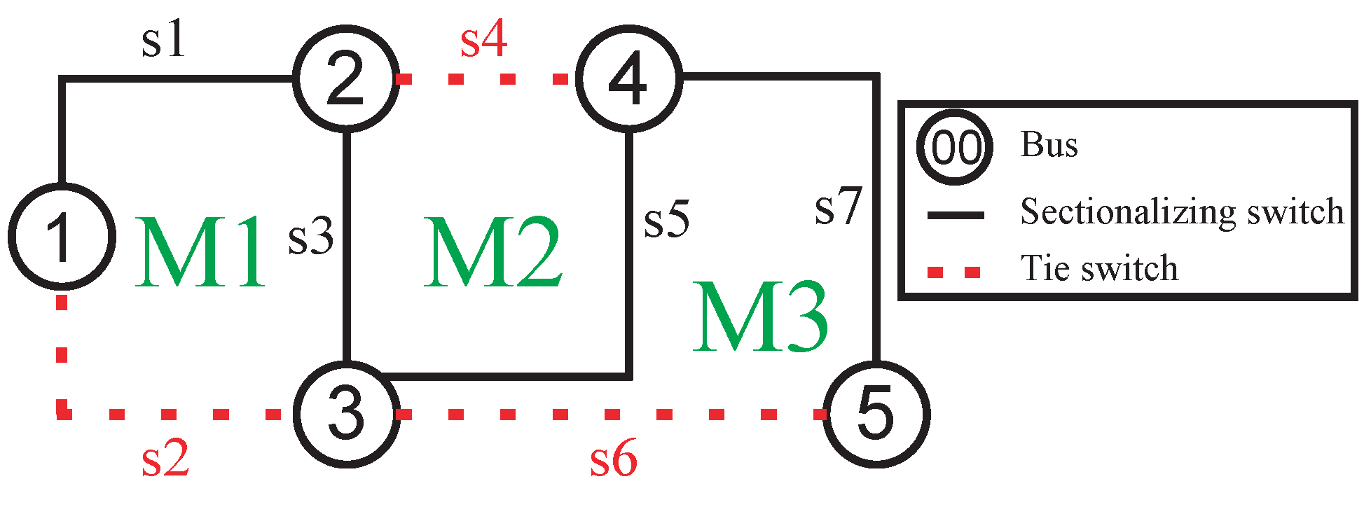
Figure 2.
Geometric and Lundy & Mees.
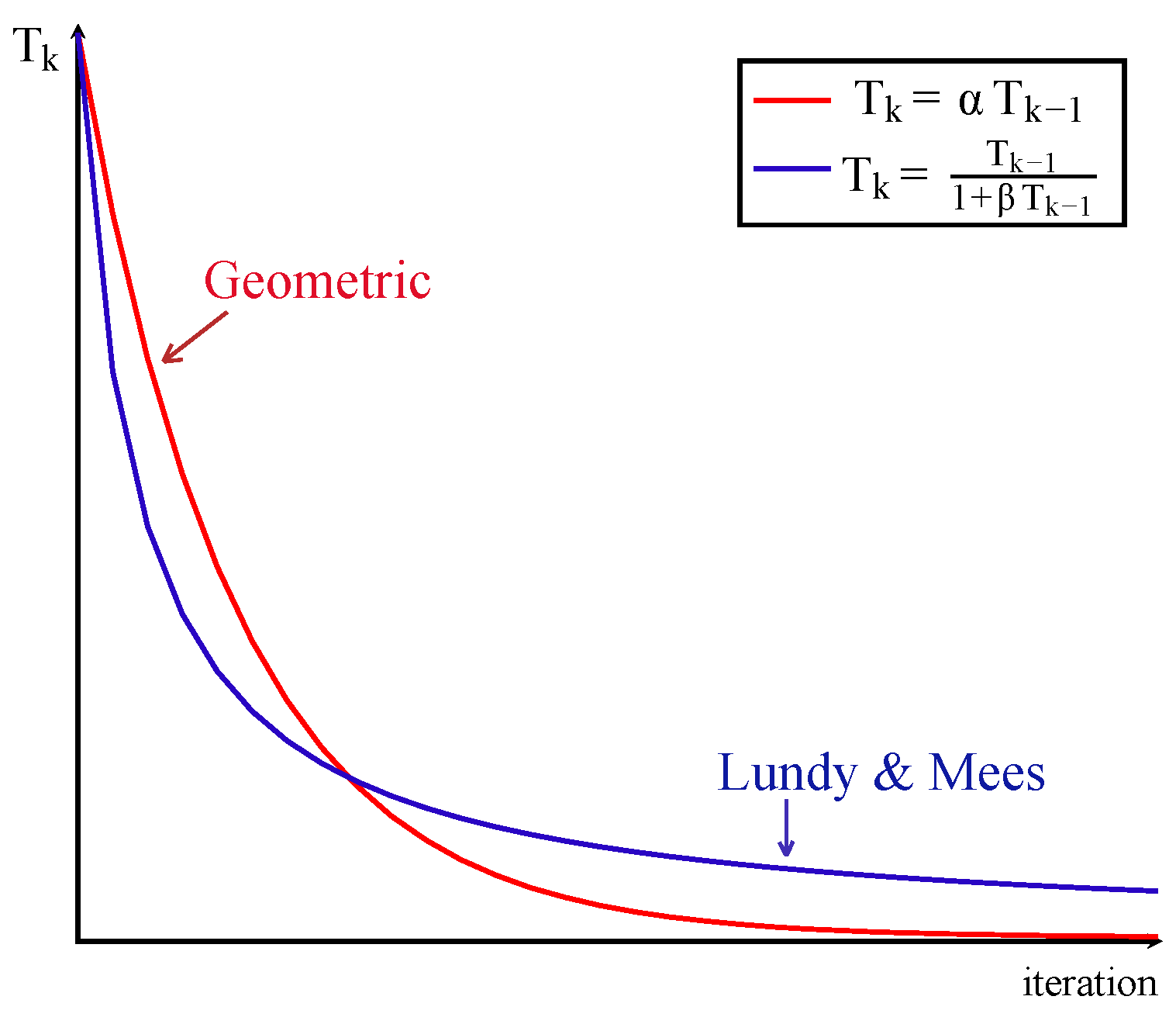
Figure 3.
GDLM mechanism.
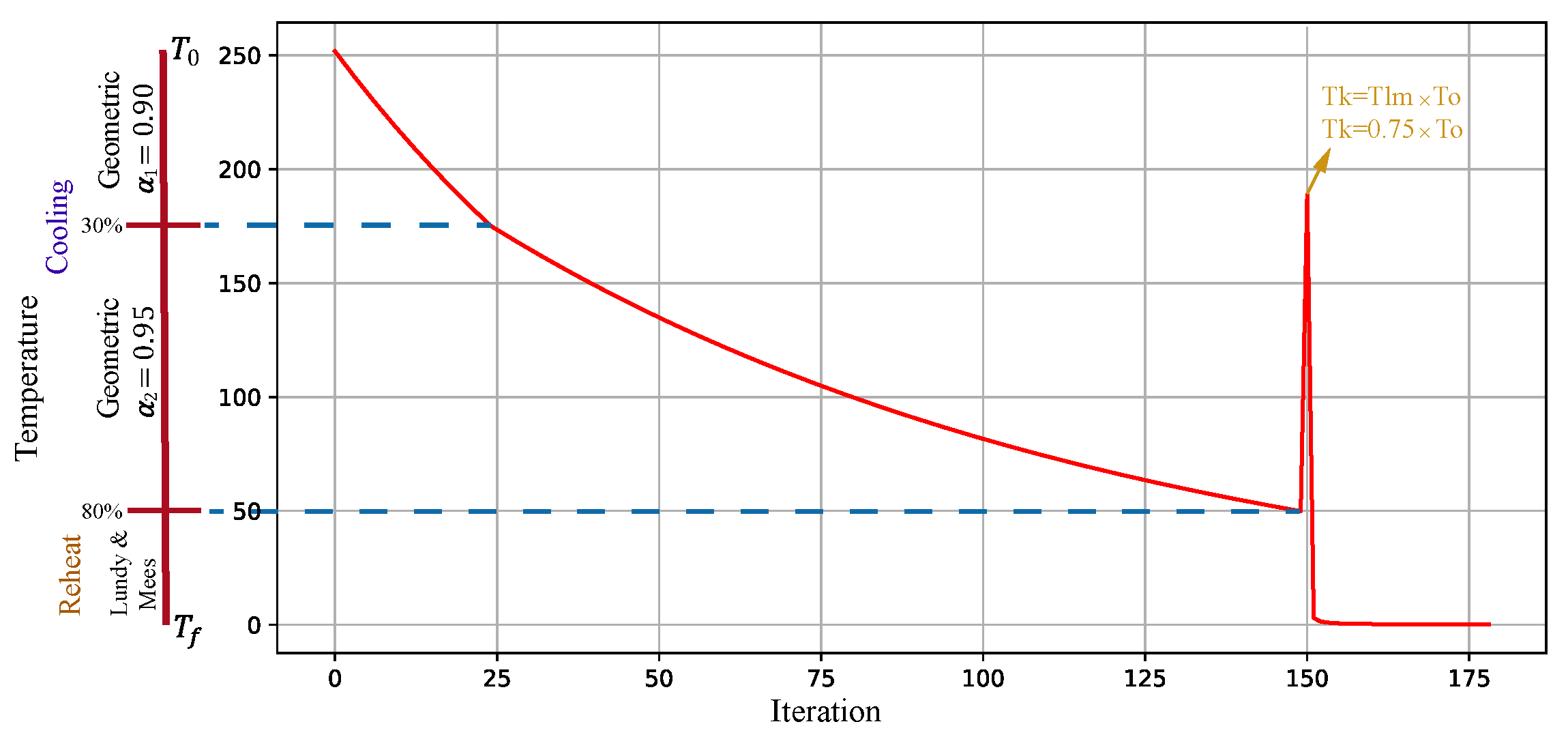
Figure 5.
Flow chart of the proposed method.
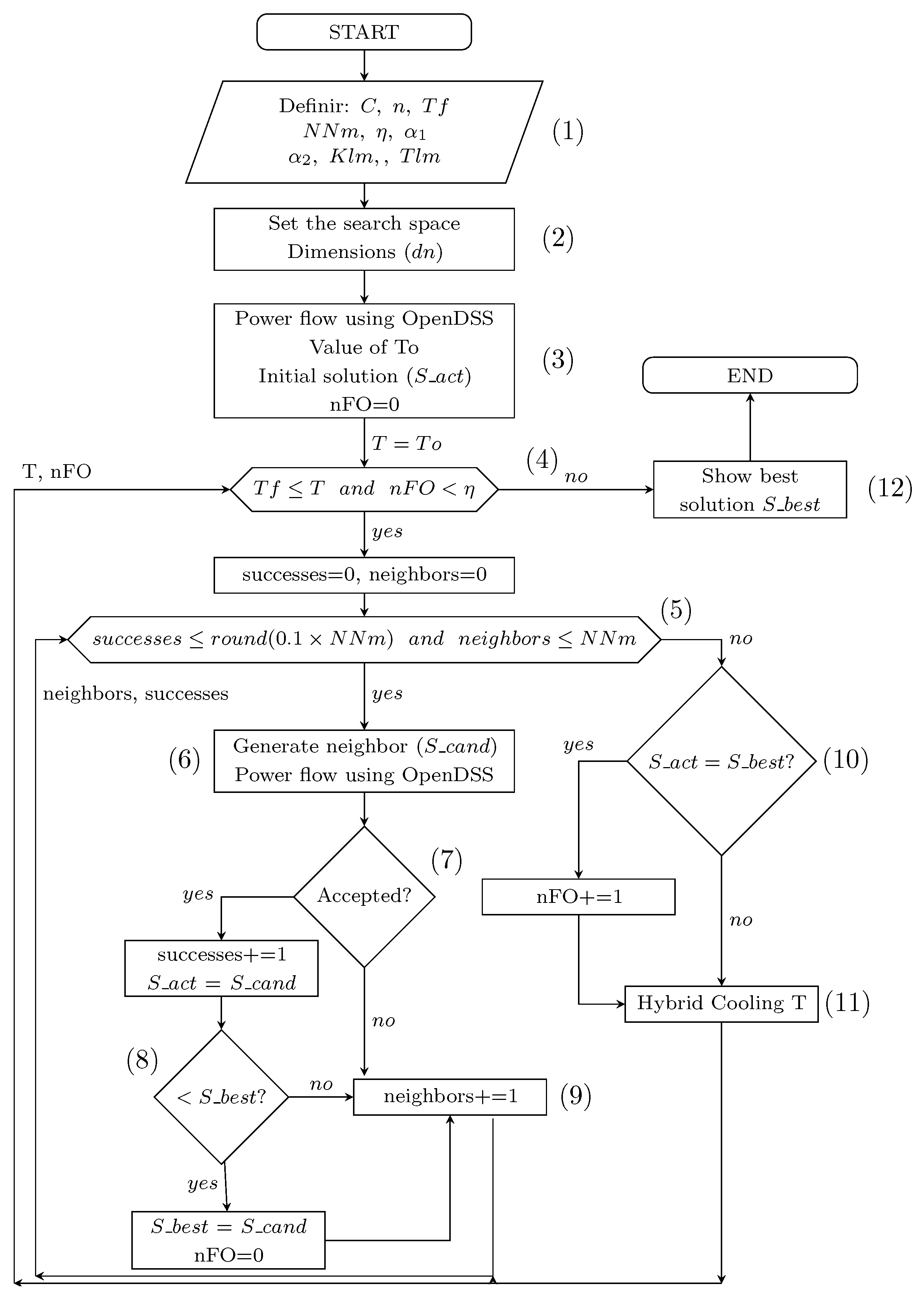
Figure 6.
Comparison of SA methods for 5 buses.
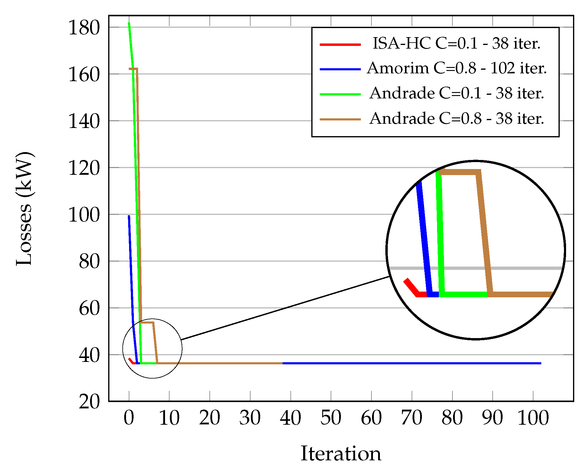
Figure 7.
Meshes of the 33 bus system.

Figure 8.
Comparison of SA methods for 33 buses.
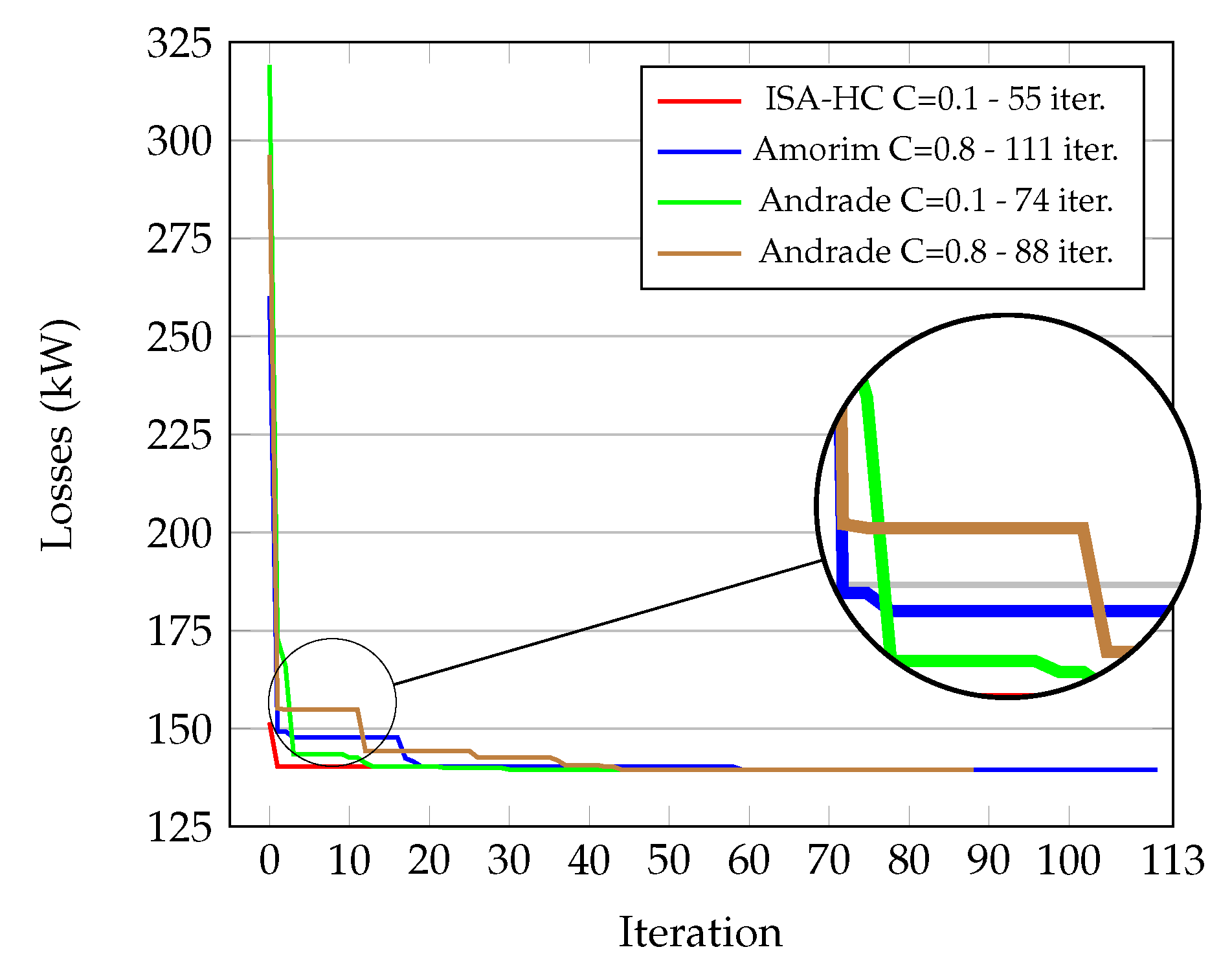
Figure 9.
Meshes of the 69-Bus system.
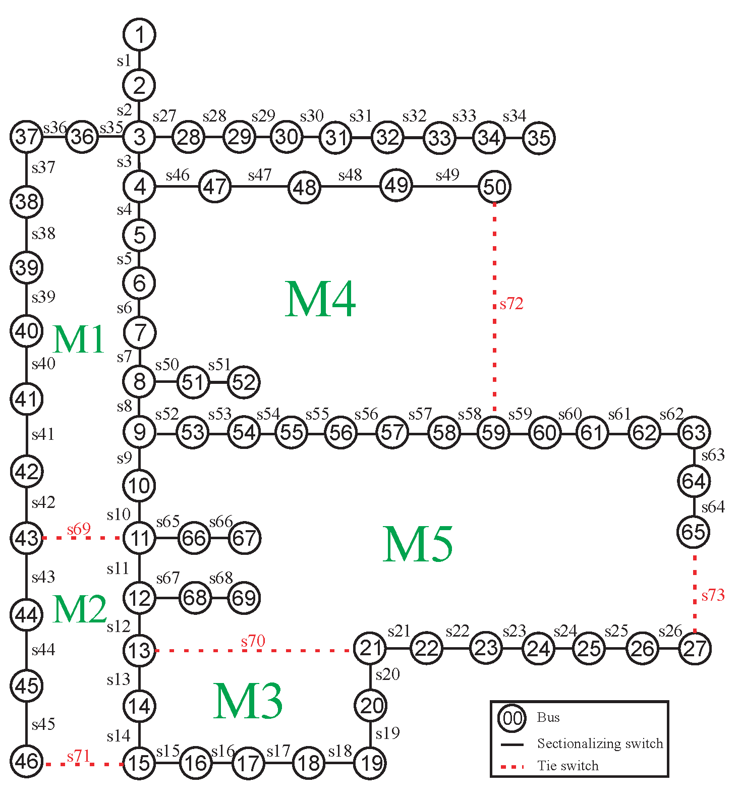
Figure 10.
Comparison of SA methods for 69 buses.
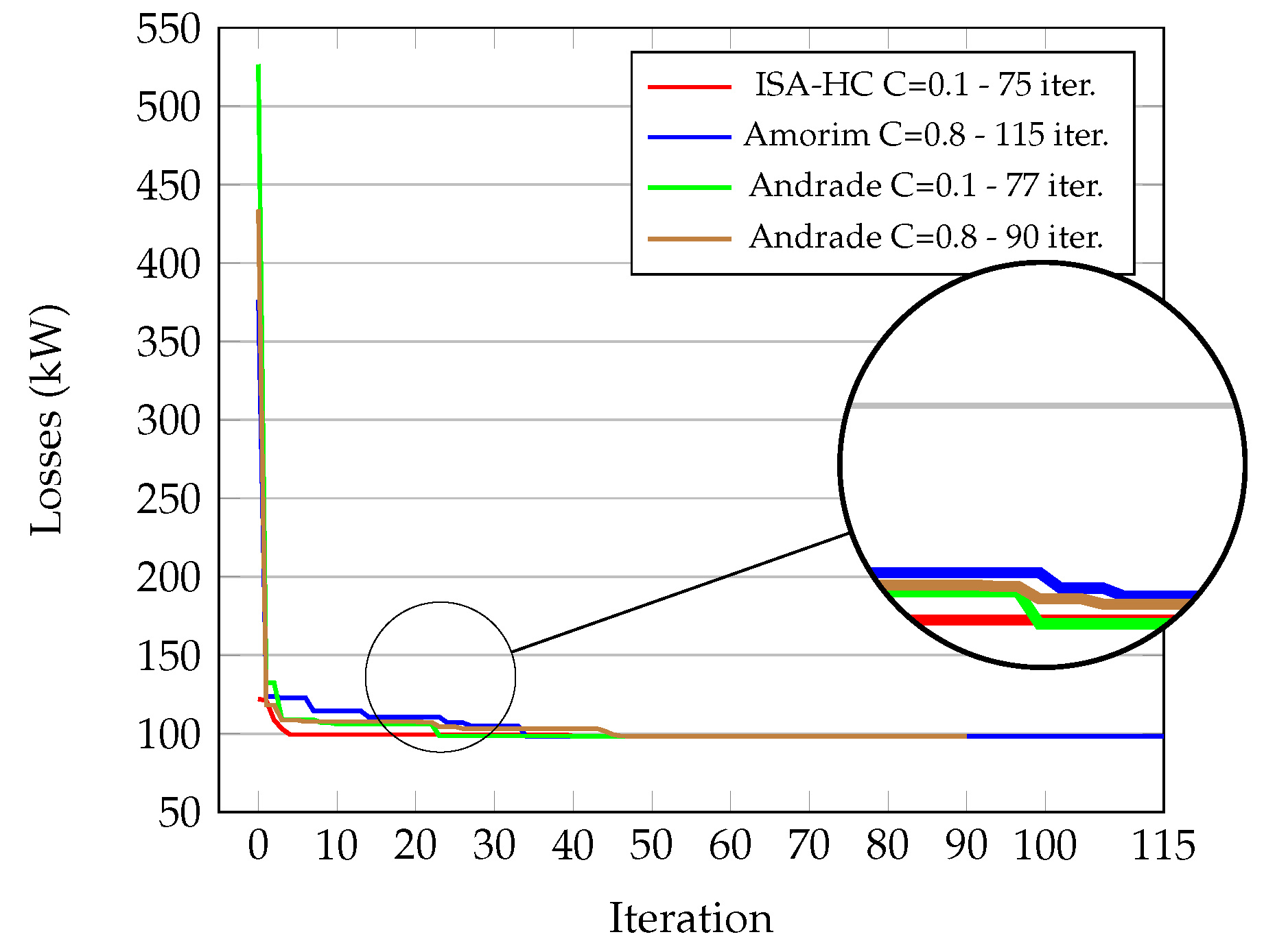
Figure 11.
Meshes of the 94-bus system.
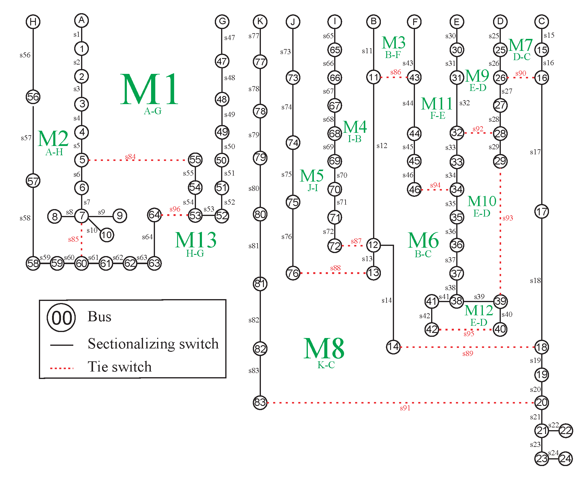
Figure 12.
Comparison of SA methods for 94 buses.
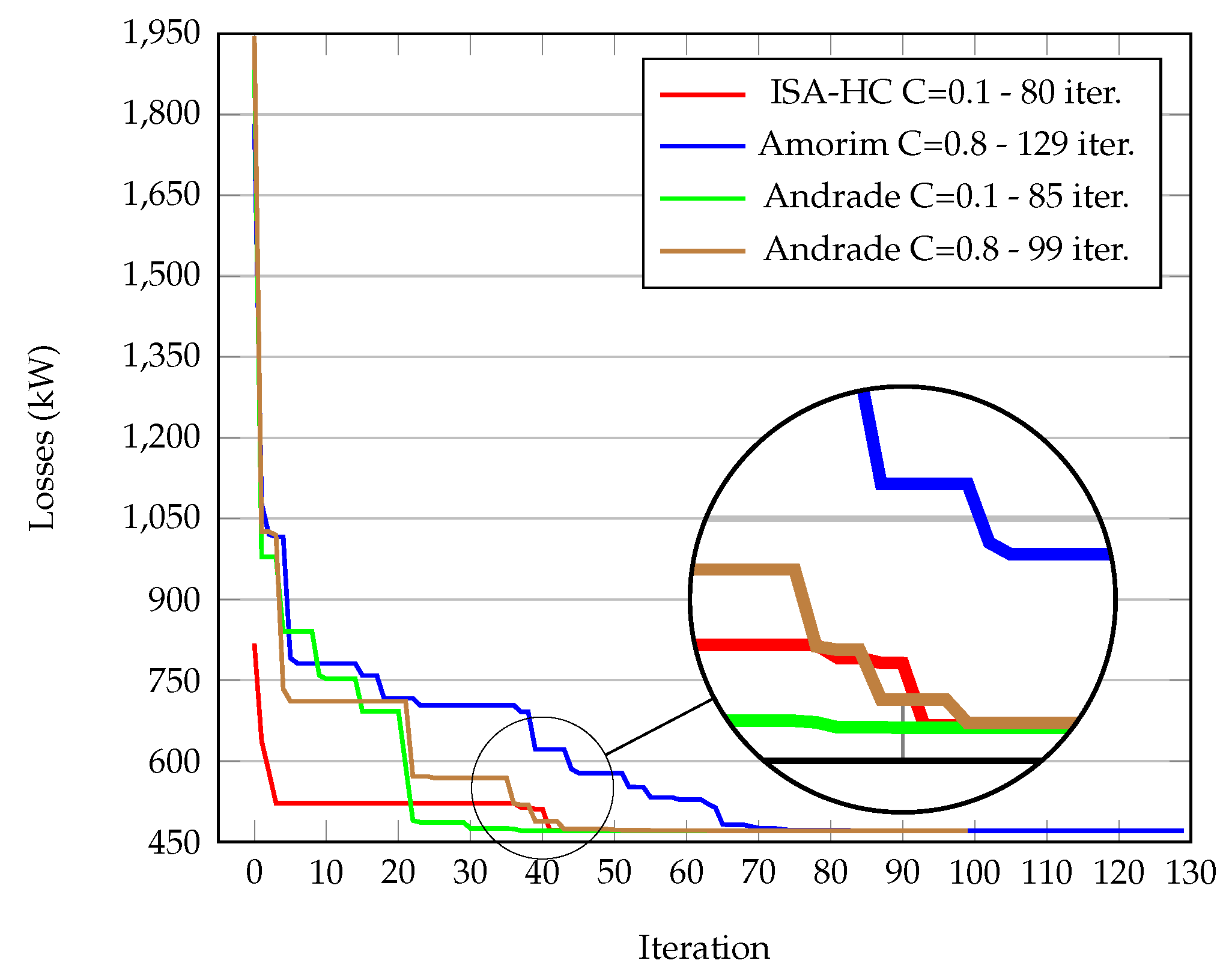

Table 1.
Results for 5 Buses—100 simulations with C constant.
| Parameter | Results | |||||||||||
|---|---|---|---|---|---|---|---|---|---|---|---|---|
| Average | Standard | Worst Solution | Best Solution | Nro | Average | Average | ||||||
| C | n | NNm | Value | Deviation | Losses | Solution | Losses | Solution | Recu. | Time | Iteration | |
| (kW) | (kW) | (kW) | (s) | |||||||||
| 0.1 | 2 | 5 | 20 | 36.248 | 0.000 | 36.248 | [3, 4, 7] | 36.248 | [3, 4, 7] | 100 | 0.51 | 38 |
| 0.1 | 2 | 5 | 15 | 36.422 | 1.737 | 53.703 | [1, 5, 7] | 36.248 | [3, 4, 7] | 99 | 0.27 | 35 |
| 0.1 | 2 | 5 | 25 | 36.248 | 0.000 | 36.248 | [3, 4, 7] | 36.248 | [3, 4, 7] | 100 | 0.39 | 46 |
| 0.1 | 2 | 10 | 20 | 36.248 | 0.000 | 36.248 | [3, 4, 7] | 36.248 | [3, 4, 7] | 100 | 0.58 | 40 |
| 0.1 | 2 | 15 | 20 | 36.248 | 0.000 | 36.248 | [3, 4, 7] | 36.248 | [3, 4, 7] | 100 | 0.95 | 45 |
| 0.1 | 3 | 5 | 20 | 36.248 | 0.000 | 36.248 | [3, 4, 7] | 36.248 | [3, 4, 7] | 100 | 0.36 | 40 |
| 0.1 | 4 | 5 | 20 | 36.256 | 0.080 | 37.053 | [1, 4, 7] | 36.248 | [3, 4, 7] | 99 | 0.35 | 68 |
Table 2.
Results for 5 Buses, n=2 —100 simulations.
| Parameter | Results | |||||||||
|---|---|---|---|---|---|---|---|---|---|---|
| Average | Standard | Worst Solution | Best Solution | Nro | Average | Average | ||||
| C | n | Value | Deviation | Losses | Solution | Losses | Solution | Recu. | Time | Iteration |
| (kW) | (kW) | (kW) | (s) | |||||||
| 0.1 | 2 | 36.248 | 0.000 | 36.248 | [3, 4, 7] | 36.248 | [3, 4, 7] | 100 | 0.51 | 38 |
| 0.2 | 2 | 36.248 | 0.000 | 36.248 | [3, 4, 7] | 36.248 | [3, 4, 7] | 100 | 0.53 | 52 |
| 0.3 | 2 | 36.248 | 0.000 | 36.248 | [3, 4, 7] | 36.248 | [3, 4, 7] | 100 | 0.51 | 73 |
| 0.4 | 2 | 36.248 | 0.000 | 36.248 | [3, 4, 7] | 36.248 | [3, 4, 7] | 100 | 0.35 | 42 |
| 0.5 | 2 | 36.248 | 0.000 | 36.248 | [3, 4, 7] | 36.248 | [3, 4, 7] | 100 | 0.37 | 60 |
| 0.6 | 2 | 36.248 | 0.000 | 36.248 | [3, 4, 7] | 36.248 | [3, 4, 7] | 100 | 0.36 | 40 |
| 0.7 | 2 | 36.248 | 0.000 | 36.248 | [3, 4, 7] | 36.248 | [3, 4, 7] | 100 | 0.35 | 46 |
| 0.8 | 2 | 36.248 | 0.000 | 36.248 | [3, 4, 7] | 36.248 | [3, 4, 7] | 100 | 0.37 | 52 |
| 0.9 | 2 | 36.248 | 0.000 | 36.248 | [3, 4, 7] | 36.248 | [3, 4, 7] | 100 | 0.36 | 53 |
Table 3.
Comparison of methods for 5 buses—100 simulations.
| Method | Global Solution |
Standard Deviation |
Solution | ||||
|---|---|---|---|---|---|---|---|
| Open Switches | Losses (kW) | ||||||
| ISA-HC (C = 0.1) | 100 | 0 | Best | 3-4-7 | 36.248 | ||
| J.Amorim-SA (2022) [22] | 100 | 0 | Best | 3-4-7 | 36.248 | ||
| R.Pegado-PSO (2019) [1] | 100 | 0 | Best | 3-4-7 | 36.248 | ||
| C.Gerez (2019) [39] | 100 | 0 | Best | 3-4-7 | 36.248 | ||
| Andrade (2018) [12] | 100 | 0 | Best | 3-4-7 | 36.248 | ||
Table 4.
Results for 33-Bus system—100 simulations with C constant.
| Parameter | Results | |||||||||||
|---|---|---|---|---|---|---|---|---|---|---|---|---|
| Average | Standard | Worst Solution | Best Solution | Nro | Average | Average | ||||||
| C | n | NNm | Value | Deviation | Losses | Solution | Losses | Solution | Recu. | Time | Iteration | |
| (kW) | (kW) | (kW) | (s) | |||||||||
| 0.1 | 2 | 20 | 20 | 139.55 | 0.00 | 139.55 | [7, 9, 37, 14, 32] | 139.55 | [7, 9, 37, 14, 32] | 100 | 4.25 | 55 |
| 0.1 | 2 | 20 | 15 | 139.56 | 0.04 | 139.95 | [7, 9, 28, 14, 32] | 139.55 | [7, 9, 37, 14, 32] | 99 | 3.38 | 61 |
| 0.1 | 2 | 20 | 25 | 139.55 | 0.00 | 139.55 | [7, 9, 37, 14, 32] | 139.55 | [7, 9, 37, 14, 32] | 100 | 4.53 | 58 |
| 0.1 | 2 | 15 | 20 | 139.55 | 0.00 | 139.55 | [7, 9, 37, 14, 32] | 139.55 | [7, 9, 37, 14, 32] | 100 | 3.57 | 53 |
| 0.1 | 2 | 25 | 20 | 139.55 | 0.00 | 139.55 | [7, 9, 37, 14, 32] | 139.55 | [7, 9, 37, 14, 32] | 100 | 4.27 | 66 |
| 0.1 | 3 | 20 | 20 | 139.55 | 0.00 | 139.55 | [7, 9, 37, 14, 32] | 139.55 | [7, 9, 37, 14, 32] | 100 | 3.96 | 61 |
| 0.1 | 4 | 20 | 20 | 139.55 | 0.00 | 139.55 | [7, 9, 37, 14, 32] | 139.55 | [7, 9, 37, 14, 32] | 100 | 3.90 | 54 |
Table 5.
Results for 33-Bus system, n = 2—100 simulations.
| Parameter | Results | |||||||||
|---|---|---|---|---|---|---|---|---|---|---|
| Average | Standard | Worst Solution | Best Solution | Nro | Average | Average | ||||
| C | n | Value | Deviation | Losses | Solution | Losses | Solution | Recu. | Time | Iteration |
| (kW) | (kW) | (kW) | (s) | |||||||
| 0.1 | 2 | 139.55 | 0.00 | 139.55 | [7, 9, 37, 14, 32] | 139.55 | [7, 9, 37, 14, 32] | 100 | 4.25 | 55 |
| 0.2 | 2 | 139.55 | 0.00 | 139.55 | [7, 9, 37, 14, 32] | 139.55 | [7, 9, 37, 14, 32] | 100 | 4.46 | 60 |
| 0.3 | 2 | 139.55 | 0.00 | 139.55 | [7, 9, 37, 14, 32] | 139.55 | [7, 9, 37, 14, 32] | 100 | 4.12 | 51 |
| 0.4 | 2 | 139.55 | 0.00 | 139.55 | [7, 9, 37, 14, 32] | 139.55 | [7, 9, 37, 14, 32] | 100 | 3.92 | 54 |
| 0.5 | 2 | 139.55 | 0.00 | 139.55 | [7, 9, 37, 14, 32] | 139.55 | [7, 9, 37, 14, 32] | 100 | 3.91 | 54 |
| 0.6 | 2 | 139.55 | 0.00 | 139.55 | [7, 9, 37, 14, 32] | 139.55 | [7, 9, 37, 14, 32] | 100 | 3.78 | 57 |
| 0.7 | 2 | 139.55 | 0.00 | 139.55 | [7, 9, 37, 14, 32] | 139.55 | [7, 9, 37, 14, 32] | 100 | 3.79 | 61 |
| 0.8 | 2 | 139.55 | 0.00 | 139.55 | [7, 9, 37, 14, 32] | 139.55 | [7, 9, 37, 14, 32] | 100 | 3.94 | 57 |
| 0.9 | 2 | 139.55 | 0.00 | 139.55 | [7, 9, 37, 14, 32] | 139.55 | [7, 9, 37, 14, 32] | 100 | 3.82 | 55 |
Table 6.
Comparison of methods for 33 buses—100 simulations.
| Method | Global Solution |
Standard Deviation |
Solution | ||||
|---|---|---|---|---|---|---|---|
| Open Switches | Losses (kW) | ||||||
| ISA-HC (C = 0.1) | 100 | 0 | Best | 7-9-14-32-37 | 139.55 | ||
| Worst | 7-9-14-32-37 | 139.55 | |||||
| J.Amorim-SA (2022) [22] | 100 | 0 | Best | 7-9-14-32-37 | 139.55 | ||
| Worst | 7-9-14-32-37 | 139.55 | |||||
| IS-BPSO (2019) [3] | 100 | 0 | Best | 7-9-14-32-37 | 139.55 | ||
| Worst | 7-9-14-32-37 | 139.55 | |||||
| Andrade; Ferreira (2018) [12] | 100 | 0 | Best | 7-9-14-32-37 | 139.55 | ||
| Worst | 7-9-14-32-37 | 139.55 | |||||
| N.H.A. Rahman (2017) [41] | 30 | 1.676 | Best | 7-9-14-32-37 | 139.55 | ||
| Worst | 7-9-13-32-37 | 143.09 | |||||
| J.Dong (2017) [42] | 20 | 1.605 | Best | 7-9-14-32-37 | 139.55 | ||
| Worst | 7-9-13-32-37 | 143.09 | |||||
Table 7.
Results for 69-Bus system—100 simulations with C constant.
| Param. | Results | |||||||||||
|---|---|---|---|---|---|---|---|---|---|---|---|---|
| Average | Standard | Worst Solution | Best Solution | Nro | Average | Average | ||||||
| C | n | NNm | Value | Deviation | Losses | Solution | Losses | Solution | Recu. | Time | Iteration | |
| (kW) | (kW) | (kW) | (s) | |||||||||
| 0.1 | 4 | 25 | 20 | 98.398 | 0.00 | 98.398 | [69, 14, 70, 55, 61] | 98.398 | [69, 14, 70, 55, 61] | 100 | 13.74 | 75 |
| 0.1 | 4 | 25 | 15 | 98.398 | 0.00 | 98.398 | [69, 14, 70, 55, 61] | 98.398 | [69, 14, 70, 55, 61] | 100 | 13.84 | 103 |
| 0.1 | 4 | 25 | 25 | 98.398 | 0.00 | 98.398 | [69, 14, 70, 55, 61] | 98.398 | [69, 14, 70, 55, 61] | 100 | 15.61 | 99 |
| 0.1 | 4 | 20 | 20 | 98.398 | 0.00 | 98.398 | [69, 14, 70, 55, 61] | 98.398 | [69, 14, 70, 55, 61] | 100 | 12.92 | 94 |
| 0.1 | 4 | 30 | 20 | 98.398 | 0.00 | 98.398 | [69, 14, 70, 55, 61] | 98.398 | [69, 14, 70, 55, 61] | 100 | 17.88 | 93 |
| 0.1 | 2 | 25 | 20 | 98.398 | 0.00 | 98.398 | [69, 14, 70, 55, 61] | 98.398 | [69, 14, 70, 55, 61] | 100 | 13.90 | 94 |
| 0.1 | 6 | 25 | 20 | 98.398 | 0.00 | 98.398 | [69, 14, 70, 55, 61] | 98.398 | [69, 14, 70, 55, 61] | 100 | 12.84 | 111 |
Table 8.
Results for 69-Bus system, n = 4—100 simulations.
| Param. | Results | |||||||||
|---|---|---|---|---|---|---|---|---|---|---|
| Average | Standard | Worst Solution | Best Solution | Nro | Average | Average | ||||
| C | n | Value | Deviation | Losses | Solution | Losses | Solution | Recu. | Time | Iteration |
| (kW) | (kW) | (kW) | (s) | |||||||
| 0.1 | 4 | 98.398 | 0.00 | 98.398 | [69, 14, 70, 55, 61] | 98.398 | [69, 14, 70, 55, 61] | 100 | 13.74 | 75 |
| 0.2 | 4 | 98.398 | 0.00 | 98.398 | [69, 14, 70, 55, 61] | 98.398 | [69, 14, 70, 55, 61] | 100 | 16.38 | 94 |
| 0.3 | 4 | 98.398 | 0.00 | 98.398 | [69, 14, 70, 55, 61] | 98.398 | [69, 14, 70, 55, 61] | 100 | 13.33 | 116 |
| 0.4 | 4 | 98.398 | 0.00 | 98.398 | [69, 14, 70, 55, 61] | 98.398 | [69, 14, 70, 55, 61] | 100 | 12.61 | 116 |
| 0.5 | 4 | 98.398 | 0.00 | 98.398 | [69, 14, 70, 55, 61] | 98.398 | [69, 14, 70, 55, 61] | 100 | 13.47 | 116 |
| 0.6 | 4 | 98.398 | 0.00 | 98.398 | [69, 14, 70, 55, 61] | 98.398 | [69, 14, 70, 55, 61] | 100 | 13.97 | 110 |
| 0.7 | 4 | 98.398 | 0.00 | 98.398 | [69, 14, 70, 55, 61] | 98.398 | [69, 14, 70, 55, 61] | 100 | 13.73 | 110 |
| 0.8 | 4 | 98.398 | 0.00 | 98.398 | [69, 14, 70, 55, 61] | 98.398 | [69, 14, 70, 55, 61] | 100 | 14.31 | 95 |
| 0.9 | 4 | 98.398 | 0.00 | 98.398 | [69, 14, 70, 55, 61] | 98.398 | [69, 14, 70, 55, 61] | 100 | 14.85 | 83 |
Table 9.
Comparison of methods for 69 buses—100 simulations.
| Method | Global Solution |
Standard Deviation |
Solution | ||||
|---|---|---|---|---|---|---|---|
| Open Switches | Losses (kW) | ||||||
| ISA-HC (C = 0.1) | 100 | 0 | Best | 55-69-14-70-61 | 98.398 | ||
| Worst | 55-69-14-70-61 | 98.398 | |||||
| J.Amorim-SA (2022) [22] | 100 | 0 | Best | 55-69-14-70-61 | 98.398 | ||
| Worst | 55-69-14-70-61 | 98.398 | |||||
| L.Pinheiro-Tabu (2022) [2] | 100 | 0 | Best | 55-69-14-70-61 | 98.398 | ||
| Worst | 55-69-14-70-61 | 98.398 | |||||
| Andrade; Ferreira (2018) [12] | 100 | 0 | Best | 55-69-14-70-61 | 98.398 | ||
| Worst | 55-69-14-70-61 | 98.398 | |||||
Table 10.
Results for 94-Bus system—100 simulations with C constant.
| Param. | Results | |||||||||||
|---|---|---|---|---|---|---|---|---|---|---|---|---|
| Aver. | Stand. | Configuration | Losses | Nro | Average | Average | ||||||
| C | n | NNm | Value | Dev. | Worst | Worst (kW) | Recu. | Time | Iteration | |||
| (kW) | best. | Best. (kW) | (s) | |||||||||
| 0.1 | 6 | 35 | 30 | 470.67 | 0 | [55, 7, 86, 72, 13, 89, 90, 83, 92, 39, 34, 42, 62] | 470.67 | 100 | 20.26 | 80 | ||
| [55, 7, 86, 72, 13, 89, 90, 83, 92, 39, 34, 42, 62] | 470.67 | |||||||||||
| 0.1 | 6 | 35 | 25 | 470.67 | 0 | [55, 7, 86, 72, 13, 89, 90, 83, 92, 39, 34, 42, 62] | 470.67 | 100 | 15.40 | 89 | ||
| [55, 7, 86, 72, 13, 89, 90, 83, 92, 39, 34, 42, 62] | 470.67 | |||||||||||
| 0.1 | 6 | 35 | 35 | 470.67 | 0 | [55, 7, 86, 72, 13, 89, 90, 83, 92, 39, 34, 42, 62] | 470.67 | 100 | 18.68 | 101 | ||
| [55, 7, 86, 72, 13, 89, 90, 83, 92, 39, 34, 42, 62] | 470.67 | |||||||||||
| 0.1 | 6 | 30 | 30 | 470.67 | 0.05 | [55, 7, 86, 72, 13, 89, 90, 82, 92, 39, 34, 42, 62] | 471.20 | 99 | 14.46 | 88 | ||
| [55, 7, 86, 72, 13, 89, 90, 83, 92, 39, 34, 42, 62] | 470.67 | |||||||||||
| 0.1 | 6 | 40 | 30 | 470.67 | 0 | [55, 7, 86, 72, 13, 89, 90, 83, 92, 39, 34, 42, 62] | 470.67 | 100 | 17.16 | 76 | ||
| [55, 7, 86, 72, 13, 89, 90, 83, 92, 39, 34, 42, 62] | 470.67 | |||||||||||
| 0.1 | 4 | 35 | 30 | 470.67 | 0 | [55, 7, 86, 72, 13, 89, 90, 83, 92, 39, 34, 42, 62] | 470.67 | 100 | 17.19 | 87 | ||
| [55, 7, 86, 72, 13, 89, 90, 83, 92, 39, 34, 42, 62] | 470.67 | |||||||||||
| 0.1 | 8 | 35 | 30 | 470.98 | 3.06 | [54, 6, 86, 72, 13, 89, 90, 83, 92, 39, 34, 42, 61] | 501.40 | 98 | 17.14 | 97 | ||
| [55, 7, 86, 72, 13, 89, 90, 83, 92, 39, 34, 42, 62] | 470.67 | |||||||||||
Table 11.
Results for 94-Bus system, n=6 — 100 simulations.
| Param. | Results | |||||||||
|---|---|---|---|---|---|---|---|---|---|---|
| Aver. | Stand. | Configuration | Losses | Nro | Average | Average | ||||
| C | n | Value | Dev. | Worst | Worst (kW) | Recu. | Time | Iteration | ||
| (kW) | best. | Best. (kW) | (s) | |||||||
| 0.1 | 6 | 470.67 | 0 | [55, 7, 86, 72, 13, 89, 90, 83, 92, 39, 34, 42, 62] | 470.67 | 100 | 20.26 | 80 | ||
| [55, 7, 86, 72, 13, 89, 90, 83, 92, 39, 34, 42, 62] | 470.67 | |||||||||
| 0.2 | 6 | 470.67 | 0 | [55, 7, 86, 72, 13, 89, 90, 83, 92, 39, 34, 42, 62] | 470.67 | 100 | 18.23 | 80 | ||
| [55, 7, 86, 72, 13, 89, 90, 83, 92, 39, 34, 42, 62] | 470.67 | |||||||||
| 0.3 | 6 | 470.67 | 0 | [55, 7, 86, 72, 13, 89, 90, 83, 92, 39, 34, 42, 62] | 470.67 | 100 | 17.57 | 84 | ||
| [55, 7, 86, 72, 13, 89, 90, 83, 92, 39, 34, 42, 62] | 470.67 | |||||||||
| 0.4 | 6 | 470.67 | 0 | [55, 7, 86, 72, 13, 89, 90, 83, 92, 39, 34, 42, 62] | 470.67 | 100 | 17.05 | 91 | ||
| [55, 7, 86, 72, 13, 89, 90, 83, 92, 39, 34, 42, 62] | 470.67 | |||||||||
| 0.5 | 6 | 470.67 | 0 | [55, 7, 86, 72, 13, 89, 90, 83, 92, 39, 34, 42, 62] | 470.67 | 100 | 24.04 | 83 | ||
| [55, 7, 86, 72, 13, 89, 90, 83, 92, 39, 34, 42, 62] | 470.67 | |||||||||
| 0.6 | 6 | 470.67 | 0 | [55, 7, 86, 72, 13, 89, 90, 83, 92, 39, 34, 42, 62] | 470.67 | 100 | 16.46 | 78 | ||
| [55, 7, 86, 72, 13, 89, 90, 83, 92, 39, 34, 42, 62] | 470.67 | |||||||||
| 0.7 | 6 | 470.67 | 0 | [55, 7, 86, 72, 13, 89, 90, 83, 92, 39, 34, 42, 62] | 470.67 | 100 | 16.69 | 112 | ||
| [55, 7, 86, 72, 13, 89, 90, 83, 92, 39, 34, 42, 62] | 470.67 | |||||||||
| 0.8 | 6 | 470.67 | 0 | [55, 7, 86, 72, 13, 89, 90, 83, 92, 39, 34, 42, 62] | 470.67 | 100 | 20.44 | 76 | ||
| [55, 7, 86, 72, 13, 89, 90, 83, 92, 39, 34, 42, 62] | 470.67 | |||||||||
| 0.9 | 6 | 470.67 | 0 | [55, 7, 86, 72, 13, 89, 90, 83, 92, 39, 34, 42, 62] | 470.67 | 100 | 17.77 | 77 | ||
| [55, 7, 86, 72, 13, 89, 90, 83, 92, 39, 34, 42, 62] | 470.67 | |||||||||
Table 12.
Comparison of methods for 94 buses—100 simulations.
| Method | Global Solution |
Standard Deviation |
Solution | ||||
|---|---|---|---|---|---|---|---|
| Open Switches | Losses (kW) | ||||||
| ISA-HC (C = 0.1) | 100 | 0 | Best | [55, 7, 86, 72, 13, 89, 90, 83, 92, 39, 34, 42, 62] | 470.67 | ||
| Worst | [55, 7, 86, 72, 13, 89, 90, 83, 92, 39, 34, 42, 62] | 470.67 | |||||
| J.Amorim-SA (2022) [22] | 100 | 0 | Best | [55, 7, 86, 72, 13, 89, 90, 83, 92, 39, 34, 42, 62] | 470.67 | ||
| Worst | [55, 7, 86, 72, 13, 89, 90, 83, 92, 39, 34, 42, 62] | 470.67 | |||||
| L.Pinheiro (2022) [2] | 100 | 0 | Best | [55, 7, 86, 72, 13, 89, 90, 83, 92, 39, 34, 42, 62] | 470.67 | ||
| Worst | [55, 7, 86, 72, 13, 89, 90, 83, 92, 39, 34, 42, 62] | 470.67 | |||||
| IS-BPSO (2019) [3] | 99 | 0.098 | Best | [55, 7, 86, 72, 13, 89, 90, 83, 92, 39, 34, 42, 62] | 470.67 | ||
| Worst | [55, 7, 86, 72, 13, 89, 90, 82, 92, 39, 34, 42, 63] | 471.37 | |||||
| Andrade (2018) [12] | 100 | 0 | Best | [55, 7, 86, 72, 13, 89, 90, 83, 92, 39, 34, 42, 62] | 470.67 | ||
| Worst | [55, 7, 86, 72, 13, 89, 90, 83, 92, 39, 34, 42, 62] | 470.67 | |||||
| J.Dong (2017) [42] | 0 | 2.1896 | Best | [55, 7, 86, 72, 13, 89, 90, 82, 92, 93, 34, 40, 62] | 471.49 | ||
| Worst | [84, 7, 86, 87, 76, 89, 90, 91, 92, 29, 34, 40, 64] | 488.68 | |||||
| Rahman (2017) [41] | 0 | 12.7050 | Best | [84, 7, 86, 72, 13, 89, 90, 83, 92, 93, 34, 40, 63] | 471.16 | ||
| Worst | [84, 85, 86, 87, 13, 89, 90, 83, 92, 93, 34, 40, 96] | 509.45 | |||||
Disclaimer/Publisher’s Note: The statements, opinions and data contained in all publications are solely those of the individual author(s) and contributor(s) and not of MDPI and/or the editor(s). MDPI and/or the editor(s) disclaim responsibility for any injury to people or property resulting from any ideas, methods, instructions or products referred to in the content. |
© 2024 by the authors. Licensee MDPI, Basel, Switzerland. This article is an open access article distributed under the terms and conditions of the Creative Commons Attribution (CC BY) license (http://creativecommons.org/licenses/by/4.0/).
Copyright: This open access article is published under a Creative Commons CC BY 4.0 license, which permit the free download, distribution, and reuse, provided that the author and preprint are cited in any reuse.


