Submitted:
06 July 2024
Posted:
08 July 2024
You are already at the latest version
Abstract
The fixed and random effects models are popular methods for identifying the causal effects of treatment. First, I introduce the two-way fixed effects model and show a class of the estimators for the random effects models. Misidentification may occur in these models due to the treatment effect heterogeneity. Then, I propose the differential error component models to address such problems while the models exclude the fixed effects of units and time periods and consider the random effects of units and time periods. Meanwhile, I present a simulation of a staggered design and revisit the application in (De Chaisemartin and D'Haultfoeuille, 2020). The results demonstrate that one additional newspaper increases the 0.31% average effect of the presidential turnout and the 1.05% average effect when the newspapers’ changes are non-negative, where the proposed estimators are robust and efficient.
Keywords:
Generalized least square
; Error component
; Fixed effects
; Random effects
; Treatment effect heterogeneity
1. Introduction
Identification of the treatment effects usually needs to exclude the fixed effects, the covariates effects, and the disturbances. The treatments may be policies, programs, or activities. The Fixed effects (FE) models and the random effects (RE) models are popular and efficient methods to identify the treatment effects, which are used to exclude the effects of units or groups and time periods. Additional information about samples is one way to obtain more precise treatment effects. The alternative is to suggest more precise estimators for treatment effects.
The two-way fixed effects (TWFE) model is an identification method with the effects of units and time periods are fixed. There has been abundant research on the TWFE model in recent years. (Goodman-Bacon, 2021) shows the negative weighted problem because the treated time periods of units in different groups are different in the TWFE model. He gives the Goodman-Bacon decomposition theorem to address such problems. De Chaisemartin and D'Haultfoeuille (2020) show an estimator to assess the robustness of the estimators for the TWFE model. They also propose an estimator that is a weighted sum of the treatment effects to avoid the negative weighted problem. (de Chaisemartin and D'Haultfoeuille, 2022) review the recent studies of the TWFE model with binary or non-binary treatment, staggered or not staggered design, and continuous or discrete time periods. The TWFE model is a popular method to identify the treatment effects of multiple time periods, and its extensions are also growing.
The one-way or two-way random effects models are the identification methods in which the effects of units or time periods are random. (Wallace and Hussain, 1969) and (Maddala, 1971) show some generalized least square (GLS) estimators of the multivariate linear regression model with three error components such as the Within estimator, the Between units estimator, and the time periods estimator. They also give the consistency, the unbiasedness, and the asymptotic normality of the estimators. (Swamy and Arora, 1972) show a class of estimators for the TWRE model, including two-stage estimators. (Baltagi, 1981) compares estimators of the OLS, the LSDV, the GLS, and six other two-stage estimators for the TWRE model by Monte-Carlo simulation. Baltagi also shows the advantages and disadvantages of these estimators in terms of both theoretical properties and application.
The question is, which is the optimal model of the above models for our daily research? Many papers have introduced the two-way effects models and their extensions. Baltagi, B. H. (2008) specifically shows the two-way effects models and discusses when we choose the TWFE or the TWRE model. (Hausman, 1978) proposes the tests for choosing the fixed e or the random effects model. However, the test result may mislead researchers into choosing an inefficient model for some applications. (Mundlak, 1978), (Chamberlain, 1984), (Hausman and Taylor, 1981), (Metcalf, 1996), and other papers show that one should test the restrictions of the fixed or random effects models before applying them to application. The RE models request that the effects of units or time periods are independent of the treatment variable and the covariates, while the models have heteroscedasticity. The FE models have endogeneity between the units, the time periods, the treatment variable, and the covariates in regression. Moreover, the FE and the RE models both have treatment effect heterogeneity. The differential models (DM) are one way to exclude heterogeneity, such as the first-difference (FD) model and the second-difference (SD) model.
Based on the above analysis, I show how the treatment effect heterogeneity causes the misidentification of the above models. Furthermore, I propose the differential error component (DRE) models that exclude the fixed effects of units and time periods and consider the random effects of units and time periods. Besides, I present a simulation of the staggered design with five groups and five time periods and revisit the application of the effects of newspapers on presidential turnout to test whether the proposed estimators are feasible and efficient.
The remainder of the paper is structured as follows. Section 2 introduces the TWFE and shows a class of estimators for the TWRE model. Section 3 proposes the DRE models. The section also shows the advantages and disadvantages of the above models. Section 4 presents a simulation and an application to compare the estimators mentioned in Section 2 and Section 3. Finally, Section 5 summarizes this paper.
2. Setups and the Misidentification in the FE and RE Models
2.1. Setups
Firstly, we show the TWFE regression model
where is the time fixed effects and is the unit fixed effects. represents the treatment effect coefficient. is a multilevel treatment statue. is the covariate matrix. is the coefficient vector of . represents the random disturbance term. The TWFE model is a popular case of linear regression models. In this TWFE regression model, the treatments in Equation (2.1) to units may exit in some time periods. The units may be treated again in the next periods. Furthermore, we should consider the heterogeneity of units and time periods in Equation (2.1) when we analyze multiple time period data, such as panel data and repeated cross-section data. Wallace and Hussain (1969) first proposed the Within estimator of the TWFE model. Liu and Sun (2019) and de Chaisemartin and D'Haultfoeuille (2020) briefly introduce the Within method.
The one-way random effect (OWRE) model: The OWRE model is a simple case of the RE models that take the units or the time period effects as the random effects. Here, I introduce the OWRE model that takes the units' effects as random effects. Defining is the identify matrix. is a vector that equals for all elements. equals to . We have the multiple linear regression model with two error components follows
where is the OWRE for unit. , , . are independent with each other. It is easy to show that the variance matrix of the disturbances is
where
Proposition 1 Let and are given, we have the GLS estimators of Equation (2.2) as And
and
Proposition 2 Let ,, The two-stage estimators of Equation (2.2) are
where .
The TWRE model: The TWRE model takes the effects of units and time periods as the random effects into the disturbance terms in the regression. Maddala (1971), Wallace and Hussain (1969), and Baltagi B. H. (2008) have introduced this linear model specifically. I will show a class of least square estimators for the TWRE model. The multiple linear regression model with three error components is
where represents the TWRE vector. It is easy to show the covariance matrix of the disturbances is
with are independent with each other. For convenient of the estimation, let
where .
Proposition 3 Let and are given. We have the GLS estimators of Equation (2.3) as
, and Proposition 3 shows all GLS estimators of Equation (2.3). The ellipses of the estimators are similar to Theorem 1.
Proposition 4 Let , the two-stage estimators of Equation (2.3) are
and
where , is the estimator of In the above, we show many estimators of the TWRE model, including , , , and . Firstly, I exclude the estimators when . These estimators are accurate only if their covariance matrix equals to the true error covariance matrix of the data. Therefore, the estimators and are omitted here. Secondly, I exclude estimators of the combination of ) that contain insufficient information about units or time periods. and are omitted. As a result, we have , and as ideal estimators for the TWRE model. These estimators are consistent in distribution because the covariance matrix strongly relates to the true covariance matrix of the data. Similarly, the above analysis is also adjusted to the differential error component models introduced in the next sections.
2.2. The Misidentification in the FE and RE Models
Misidentification may occur in FE and RE models due to the treatment effect heterogeneity. I introduce the negative weighted problem before showing heterogeneous treatment effects in these models. The negative weighted problem comes from the treatment effect heterogeneity between units or time periods. Goodman-Bacon (2021) demonstrates the negative weighted problem by a staggered design with three groups and three time periods. He shows the Goodman-Bacon decomposition theorem that considers the treatment effect heterogeneity over time periods. Figure 1 demonstrates that the negative weighted problem is caused by Case 4, which is a two-by-two DID with Group 1 and Group 2. This is the other view of the treatment effect heterogeneity compared to the one in Goodman-Bacon (2021). The heterogeneity of this 2x2 DID come from the difference in the treatment effects over time periods in the early treated Group 2. De Chaisemartin and D'Haultfoeuille (2020) show the negative weighted problem in the TWFE model. They proposed an estimator of a weighted sum of the treatment effects when the treatment status changes. The estimator is used to avoid the treatment effect heterogeneity over time periods.
The RE models take the heterogeneity of treatment effects as part of the error components. These are misleading to the estimation of the treatment effects because the distribution of the treatment effect heterogeneity is not given or pre-estimated as normality. Therefore, the estimates of the TWRE are not consistent but may be more robust than the TWFE model. The OWRE model that takes the time period effects as fixed and the unit effects as random is even worse than the TWFE or TWRE models. Accordingly, the estimation results of the OWRE in Section 4 are overestimated or negative.
3. The Differential Error Component Model
The OWRE or the TWRE models take unit effects or time period effects as random effects in Section 2. It is reasonable that the disturbances of a large panel have asymptotic normality in these models. Meanwhile, the regression models need intercept terms to avoid fixed effects on the treatment effect heterogeneity. However, it is hard to find such fitted terms because of the differences in fixed effects between units or time periods. Here, I introduce the differential models that exclude the fixed effects in regression. The FD model gives the trends of change in the treatment effects. The SD model, also called FD of FD’s, gives the characteristic of change in treatment effects. The FD is similar to speed in Physics, while the SD is similar to acceleration. Next, I take the RE models into estimation to avoid random effects to the treatment effects. This three-stage estimation excludes the fixed effects in the first step and the random effects in the last two steps. The differential error component models that combine the differential models and the error component models are also called as the differential random effects (DRE) model.
3.1. The First Differential Random Effects (FDRE) Models
Firstly, we have the FD model
with . The covariance matrix of the disturbances does not discussed here if we combine Equation (2.1) and Equation (3.1) as the FD model. I show no assumptions about the disturbances in Equation (2.1). Without loss of generality, I assume the disturbances in Equation (3.1) satisfy the following assumption.
Assumption 3.1 The disturbances in Equation (3.1) have the error components as ().
The first differential two-way random effects (FDTW) model: The TWRE model mentioned in Section 2 under Assumption 3.1 follows
where , The covariance matrix of in Equation (3.2) is
with . are independent with each other. Furthermore, we have
where , , , , , , , , , .
Lemma 1 are symmetric and idempotent. and are orthogonal with each other. And .
Lemma 2 The rank of are and 1. And .
Theorem 1 Let and are given, we have the GLS estimators of Equation (3.2) as
, and
Corollary 1Corollary 2 Let then , and are asymptotic normal with the expectation and the variance matrix corresponding to Corollary 1.
In fact, we cannot get the true while Theorem 1 assumes the variance matrix of the disturbances are given. On the one hand, we can give these variances by empirical method. One simple way is to let . We have or for the most estimators in Theorem 1 though the estimators are unbiased and asymptotic normal. These estimators are simplified as and with . On the other hand, we can estimate these variances by methods like the two-stage estimation, see also Baltagi, B. H. (2008). We have the following estimators of the disturbances for Equation (3.2)
Defining the estimator of as
where Corollary 3 are unbiased. And let conditions in Corollary 2 holdwe have
Corollary 4 Let conditions in Corollary 2 hold, we have are independent with, and are independent with each other.
Therefore, under Corollaries 3-4, we can estimate for the estimators with the unknown true variances of the error components in Theorem 1.
Theorem 2 Let , the two-stage estimators of Equation (3.2) are
and
where .
These estimators, characterized by units or time periods, focus on different information in estimation as estimators in Theorem 1 do. The unbiasedness of the above estimators follows
Corollary 5 Let conditions in Corollary 2 hold, then and are unbiased estimators of .
The first differential one-way random effects (FDOW) model
Assumption 3.2 The disturbances in Equation (3.1) have the error components as ().
The OWRE model mentioned in Section 2 under Assumption 3.2 follows
where The covariance matrix of in Equation 3.3) is Defining , , , . We have
Theorem 2 Let conditions hold in Proposition 3 and Assumption 3.2, the estimators and their asymptotic properties of the FDOW model in Equation (3.3) are similar to Propositions 1-2 and Corollaries 1-5.
3.2. The Second Differential Random Effects (SDRE) Models
The SD model gives the characteristic of change in treatment effects. It also excludes the fixed effects of units and time periods. We have the SD model as follows.
where , and with . The covariance matrix of the disturbances does not discuss here if we combine Equation (2.1) and Equation (3.4) as the SD model. Without loss of generality, I assume the disturbances in Equation (3.4) satisfy the following assumption.
Assumption 3.3 The disturbances in Equation (3.4) have the error components as ().
The second differential two-way random effects (SDTW) model: The TWRE model mentioned in Section 2 under Assumption 3.3 follows
where , The covariance matrix of in Equation (3.5) is
with . are independent with each other. Furthermore, defining , , , , , , , , , . We have
Corollary 6 Let conditions hold in Corollary 2 and Assumption 3.3, the estimators and their asymptotic properties of the SDTW model in Equation (3.5) are similar to Theorem 1 and Corollaries 1-5.
The second differential one-way random effects (SDOW) model
Assumption 3.4 The disturbances in Equation (3.4) have the error components as ().
The OWRE model mentioned in Section 2 under Assumption 3.4 follows
where . The covariance matrix of in Equation (3.6) is Defining , , , . We have
Corollary 7 Let conditions hold in Proposition 2 and Assumption 3.4, the estimators and their asymptotic properties of the SDOW model in Equation (3.6) are similar to Propositions 1-2 and Corollaries 1-5.
The Higer-order DRE models: The SDRE and FDRE models exclude the fixed effects in regression. They apply to different practical samples. However, the third or other higher-order differences for the error component model are unsuitable for identifying causal effects. These models need strong restrictions on data and will waste a lot of information in the sample. We omitted them here.
The estimations of the DRE models exclude fixed effects and consider random effects. It is more robust than the TWFE, the Differential, or the RE models. The models or estimators which we adopt in estimation depend on the data. The following section will show the optimal model for a given panel.
3.3. Comparisons of the Above Identifications
We have discussed the advantages and disadvantages of the FE, the RE, and the DRE models in the above. The TWFE model has endogeneity between units, time periods, and regressors, assuming that the disturbances have asymptotic normality. There is no need for intercept terms in regression. However, the TWFE model may have some negative weights in estimation, which causes the treatment effects weights to be negative. Secondly, the RE models need intercept terms so that the exceptions of error components are equal to 0. The RE model requests independence between units, time periods, and regressors. Moreover, the DRE models exclude fixed effects and consider random effects. The DRE models are better than the RE models or the FE models in large samples.
Here, I show the optimal model for different panels in our daily research. I also transform the unbalanced data to the balanced data by methods like interpolation. These data are characterized by the size of samples and the length of time periods. Table 1 shows the optimal model for different types of data.
4. Simulation and Application
Here, I show some classes of estimators for identifying the treatment effects. These estimators mentioned in Section 2 and Section 3 are classified by the models of the FE, the RE, and the DRE. The simulation data is a staggered design between five groups over five time periods as depicted in Figure 2. There are four groups that are treated at different time periods and one untreated group. The outcomes matrix and the treatment status matrix are
In this staggered design, the treatment effects of four groups are (10, 15, 5, 12.5). The ATT is 10.625 without the heterogeneity over time periods. On the other hand, the treatment effects of 10 2x2 DIDs are (10, 10, 10, 10, 15, 15, 15, 5, 5, 12.5) under the Goodman-Bacon decomposition theorem. The ATT is 10.75 under the theorem. I use these two ATTs as the best values to compare with estimates of the methods mentioned in Section 2 and Section 3. Table 2, Table 3 and Table 4 demonstrate that the estimates of the RE models are not ideal because of the ignorance of the fixed effects, especially in such a small sample. However, the estimates of the DRE models are more accurate by excluding the fixed effects at the first step.
The other data comes from Gentzkow and Shapiro (2011) about the effects of the entries and exits of the newspapers on the presidential turnout from 1872 to 1928. Firstly, I use interpolation for the default values where the lead value and lag value are not default. The balanced data are expanded from 847 groups to 905 groups. Secondly, there are negative values in the changes in the newspapers over time periods. I estimate the treatment effects of newspaper changes and the treatment effects of the newspapers' positive changes. Gentzkow and Shapiro (2011) use the FD method to regress the country in which the number of newspapers is positive, while this paper highlights the changes in the newspapers are non-negative. Therefore, we have the straight and positive effects of the newspaper changes on presidential turnout.
In Table 2, Table 3 and Table 4, the TWFE and the FD method estimates are not significant for the heteroscedasticity in regression, while the SD method is significant. Table 2, Table 3 and Table 4 also demonstrate that the OWRE method estimates are insignificant. The SDOW method is accurate, and the average effect of the treatment is about 0.25%. The estimates of the TWRE method are significant, but the TWRE method may not be accurate for the treatment effect heterogeneity. The estimates of the FDTW method are inconsistent, while the estimates of the SDTW method are significant and consistent. In a word, the results in Table 2, Table 3 and Table 4 demonstrate that one additional newspaper increases the 0.31% average effect of the presidential turnout. Furthermore, there are 12% negative changes in the newspapers in the data. These negative changes may cause the underestimation of the treatment effects. Here, I drop such negative changes and estimate the rest in the newspapers. The TWFE, the OWRE, the TWRE, and the FDTW estimates are about 1.32%, 1.26%, 1.23%, and 1.05%, while the last three methods are significant. The FDTW method is better than others for excluding the fixed and the random effects. Hence, one additional newspaper increases the 1.05% average effect of the presidential turnout when the newspapers’ changes are all non-negative.
5. Conclusion
Identification of the treatment effects usually needs to exclude the fixed effects, the covariates effects, and the disturbances. The fixed and random effects models are popular methods for identifying the causal effects of treatment. Based on abundant theoretical and empirical research of the fixed or the random effects models, this paper introduces explicitly a class of the least square estimators of the OWRE, and the TWRE models. Then, the paper depicts how the treatment effect heterogeneity causes the misidentification of these models. Further, I propose the DRE models, such as the FDOW, the FDTW, the SDOW, and the SDTW models, to address such problems. These models exclude the fixed effects of units and time periods and consider the random effects of units and time periods. Besides, the estimators of the DRE models are consistent and unbiased. The asymptotic properties of these estimators are shown in the Appendix. Meanwhile, I show the staggered design with five groups and revisit the application about the effects of newspapers on presidential turnout. The results demonstrate that the estimates of the DRE models are more significant and robust than the FD, SD, FE, or RE models. I leave the best estimators of the above models for a given data as further research.
Appendix A. Proofs
A.1 Proof of Theorem 1
Firstly, we have the GLS estimator of Equation (3.2) under Lemma 1-2 follows
where Secondly, we have following four equations by multiplying Equation (3.2) with
where . Under Lemma 1-2, the GLS estimators of Equation (A1) are where is the Between units estimator and is the Between time periods estimator. charactered nothing but constant is too large to become significant. These estimators are omitted for insufficient regression information. Furthermore, we obtain other 10 GLS estimators with combination of equations in Equation (10). Here I show the proof of while the proof of other estimators is similar. We have partitioned matrix equation by combining first three equations in Equation (A2) as follow.
The GLS estimator of the partitioned matrix equation is
where is generalized inverse of . And
Similarly, we have other GLS estimators for partitioned matrix equation of combination of equations in Equation (A2) as
A.2 Proof of Corollary 1
The unbiasedness and the variance matrix of and are similar with the above proof and are omitted here.
A.3 Proof of Corollary 3
Secondly, we have
where is a symmetric and idempotent matrix. The quadratic form with normal vectors has a chi-square distribution if its matrix is symmetric and idempotent. Hence,
where
A.4 Proof of Corollary 4
Given that has a quadratic form with normal vectors, It is easy to show,
Then are independent with and are independent with each other under the properties of linear independence of the quadratic form with normal vectors.
A.5 Proof of Theorem 2
The proof of Theorem 2 can be obtained directly under Theorem 1 and Corollaries 3-4.
A.6 Proof of Corollary 5
Appendix B. Supplementary data
Supplementary material related to this manuscript can be found in the Supplementary Material.zip.
References
- Abadie, A. Semiparametric difference-in-differences estimators. The review of economic studies 2005, 72, 1–19. [Google Scholar] [CrossRef]
- Angrist, J. D.; Imbens, G. W. Two-stage least squares estimation of average causal effects in models with variable treatment intensity. Journal of the American statistical Association 1995, 90, 431–442. [Google Scholar] [CrossRef]
- Arkhangelsky, D.; Imbens, G. W. Doubly robust identification for causal panel data models. The Econometrics Journal 2022, 25, 649–674. [Google Scholar] [CrossRef]
- Baltagi, B. H. Pooling: An experimental study of alternative testing and estimation procedures in a two-way error component model. Journal of Econometrics 1981, 17, 21–49. [Google Scholar] [CrossRef]
- Baltagi, B. H., and Baltagi, B. H. (2008), Econometric analysis of panel data (Vol. 4): Springer.
- Baltagi, B. H.; Song, S. H.; Jung, B. C. The unbalanced nested error component regression model. Journal of Econometrics 2001, 101, 357–381. [Google Scholar] [CrossRef]
- Baltagi, B. H., Song, S. H., and Jung, B. C. A comparative study of alternative estimators for the unbalanced two-way error component regression model. The Econometrics Journal 2002, 5, 480–493. [Google Scholar] [CrossRef]
- Casella, G., and Berger, R. L. (2002), Statistical Inference: Thomson Learning.
- Chamberlain, G. Panel data. Handbook of econometrics 1984, 2, 1247–1318. [Google Scholar]
- de Chaisemartin, C., and d'Haultfoeuille, X. (2020), "Two-way fixed effects regressions with several treatments," arXiv preprint arXiv:2012.10077.
- De Chaisemartin, C., and d’Haultfoeuille, X. Two-way fixed effects estimators with heterogeneous treatment effects. American Economic Review 110, 2964–2996. [CrossRef]
- ---. Two-way fixed effects and differences-in-differences with heterogeneous treatment effects: A survey. The Econometrics Journal 26, C1–C30. [CrossRef]
- Gentzkow, M., Shapiro, J. M., and Sinkinson, M. The effect of newspaper entry and exit on electoral politics. American Economic Review 101, 2980–3018. [CrossRef]
- Goodman-Bacon, A. Difference-in-differences with variation in treatment timing. Journal of Econometrics 2021, 225, 254–277. [Google Scholar] [CrossRef]
- Hausman, J. A. Specification tests in econometrics. Econometrica: Journal of the econometric society 1978, 1251–1271. [Google Scholar] [CrossRef]
- Hausman, J. A., and Taylor, W. E. Panel data and unobservable individual effects. Econometrica: Journal of the econometric society 1981, 1377–1398. [Google Scholar]
- Imai, K., and Kim, I. S. On the use of two-way fixed effects regression models for causal inference with panel data. Political Analysis 2021, 29, 405–415. [Google Scholar] [CrossRef]
- Liu, C., and Sun, Y. A simple and trustworthy asymptotic t test in difference-in-differences regressions. Journal of Econometrics 210, 327–362. [CrossRef]
- Maddala, G. S. The use of variance components models in pooling cross section and time series data, Econometrica: Journal of the econometric society 1971, 341–358. [Google Scholar] [CrossRef]
- Metcalf, G. E. Specification testing in panel data with instrumental variables. Journal of Econometrics 1996, 71, 291–307. [Google Scholar] [CrossRef]
- Mundlak, Y. On the pooling of time series and cross section data. Econometrica: Journal of the econometric society 1978, 69–85. [Google Scholar] [CrossRef]
- Pereda-Fernández, S. Copula-Based Random Effects Models for Clustered Data. Journal of Business & Economic Statistics 2021, 39, 575–588. [Google Scholar] [CrossRef]
- Swamy, P., and Arora, S. S. The exact finite sample properties of the estimators of coefficients in the error components regression models. Econometrica: Journal of the econometric society 1972, 261–275. [Google Scholar]
- Van der Vaart, A. W. (2000), Asymptotic statistics (Vol. 3): Cambridge university press.
- Wallace, T. D., and Hussain, A. The use of error components models in combining cross section with time series data. Econometrica: Journal of the econometric society 1969, 55–72. [Google Scholar]
- Wooldridge, J. M. (2021), "Two-way fixed effects, the two-way mundlak regression, and difference-in-differences estimators," Available at SSRN 3906345.
Figure 1.
Four cases of the decomposition theorem.
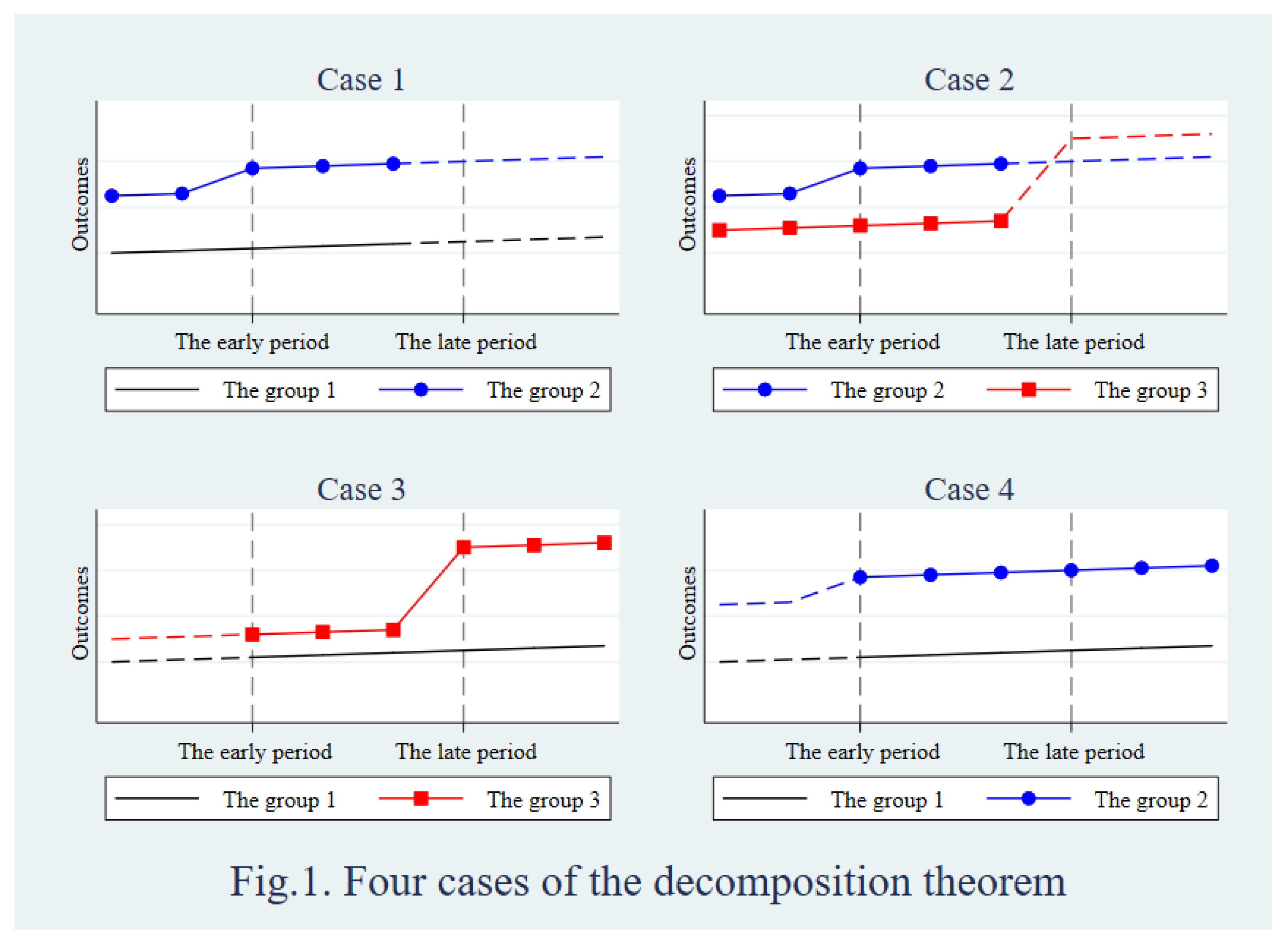
Figure 2.
The outcomes changes of the five groups.
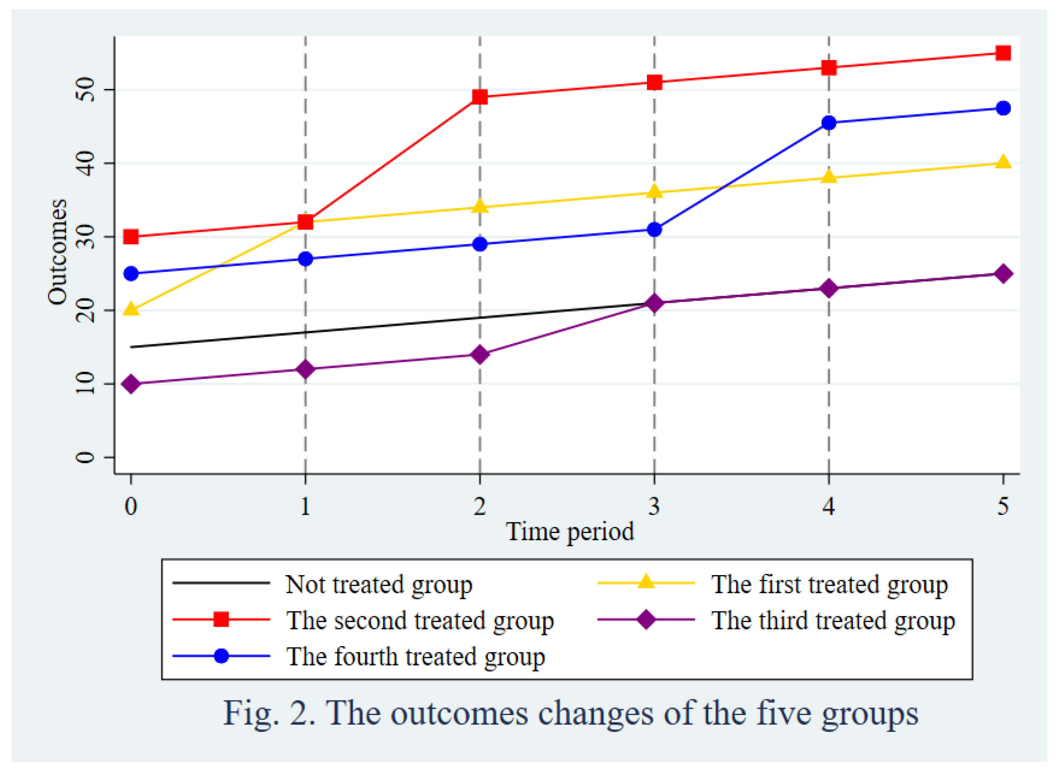

Table 1.
The optimal model for different panels.
| Small sample | Large sample | |
| Short time periods | TWFE/DM | TWFE/DRE |
| Long time periods | TWFE/DRE | TWRE/DRE |
Table 2.
The estimations of the TWFE, the FD, and the SD.
| Staggered design | Newspapers for all changes | Newspapers for positive changes | |
| TWFE | 10.50 | 0.0032 | 0.0132 |
| (0.1095) | (0.0613) | (0.2130) | |
| FD | 12.63 | 0.0019 | -0.0065 |
| (0.0000) | (0.0785) | (0.9644) | |
| SD | 10.42 | 0.0025 | 0.0036 |
| (0.0000) | (0.0346) | (0.4448) |
Table 3.
The estimations of the OWRE, the FDOW and the SDOW.
| Staggered design | ||||
| OWRE | 15.50 | 16.35 | 15.52 | 16.34 |
| (0.0000) | (0.0000) | (0.0000) | (0.0000) | |
| FDOW | 10.63 | 12.04 | 10.63 | 12.09 |
| (0.0000) | (0.0000) | (0.0000) | (0.0000) | |
| SDOW | 10.31 | 11.13 | 11.13 | 10.31 |
| (0.0000) | (0.0000) | (0.0000) | (0.0000) | |
| Newspapers for all changes | ||||
| OWRE | -0.0241 | 0.0018 | 0.0018 | 0.0032 |
| (1.0000) | (0.0399) | (0.0475) | (0.0021) | |
| FDOW | 0.0026 | 0.0005 | 0.0039 | -0.0010 |
| (0.0292) | (0.3425) | (0.0018) | (0.7595) | |
| SDOW | 0.0024 | 0.0027 | 0.0024 | 0.0028 |
| (0.0414) | (0.0226) | (0.0420) | (0.0217) | |
| Newspapers for positive changes | ||||
| OWRE | -0.0936 | 0.0126 | 0.0126 | 0.0115 |
| (1.0000) | (0.0021) | (0.0026) | (0.0049) | |
| FDOW | -0.0088 | -0.023 | -0.0031 | -0.0285 |
| (0.8542) | (0.9996) | (0.6504) | (1.0000) | |
| SDOW | 0.0011 | 0.0031 | 0.0055 | -0.0014 |
| (0.4523) | (0.3606) | (0.2673) | (0.5601) | |
Table 4.
The estimations of TWRE, FDTW and SDTW.
| Staggered design | ||||||||
| TWRE | 10.50 | 18.26 | 18.26 | 10.56 | 10.56 | 18.26 | 18.26 | 10.50 |
| (0.0000) | (0.0000) | (0.0000) | (0.0000) | (0.0000) | (0.0000) | (0.0000) | (0.0000) | |
| FDTW | 10.63 | 11.50 | 10.63 | 11.50 | 10.63 | 10.63 | 10.63 | 11.53 |
| (0.0000) | (0.0000) | (0.0000) | (0.0000) | (0.0000) | (0.0000) | (0.0000) | (0.0000) | |
| Newspapers for all changes | ||||||||
| TWRE | 0.0032 | 0.0022 | 0.0022 | 0.0023 | 0.0032 | 0.0023 | 0.0032 | 0.0032 |
| (0.0014) | (0.0137) | (0.0137) | (0.0113) | (0.0018) | (0.0113) | (0.0018) | (0.0014) | |
| FDTW | 0.0026 | 0.0037 | 0.0037 | 0.0037 | 0.0026 | 0.0037 | 0.0026 | 0.0026 |
| (0.0179) | (0.0012) | (0.0012) | (0.0012) | (0.0181) | (0.0012) | (0.0179) | (0.0181) | |
| SDTW | 0.0031 | 0.0030 | 0.0030 | 0.0031 | 0.0031 | 0.0030 | 0.0031 | 0.0031 |
| (0.0079) | (0.0084) | (0.0084) | (0.0084) | (0.0080) | (0.0084) | (0.0080) | (0.0078) | |
| Newspapers for positive changes | ||||||||
| TWRE | 0.0115 | 0.0043 | 0.0043 | 0.0123 | 0.0033 | 0.0123 | 0.0033 | 0.0115 |
| (0.0215) | (0.2128) | (0.2128) | (0.0140) | (0.2739) | (0.0140) | (0.2739) | (0.0215) | |
| FDTW | 0.0075 | 0.0102 | 0.0105 | 0.0107 | 0.0066 | 0.0110 | 0.0069 | 0.0071 |
| (0.1606) | (0.0786) | (0.0732) | (0.0691) | (0.1885) | (0.0642) | (0.1783) | (0.1701) | |
| SDTW | 0.0050 | 0.0084 | 0.0084 | 0.0085 | 0.0050 | 0.0085 | 0.0050 | 0.0051 |
| (0.2694) | (0.1475) | (0.1475) | (0.1446) | (0.2739) | (0.1445) | (0.2737) | (0.2695) | |
Disclaimer/Publisher’s Note: The statements, opinions and data contained in all publications are solely those of the individual author(s) and contributor(s) and not of MDPI and/or the editor(s). MDPI and/or the editor(s) disclaim responsibility for any injury to people or property resulting from any ideas, methods, instructions or products referred to in the content. |
© 2024 by the authors. Licensee MDPI, Basel, Switzerland. This article is an open access article distributed under the terms and conditions of the Creative Commons Attribution (CC BY) license (http://creativecommons.org/licenses/by/4.0/).
Copyright: This open access article is published under a Creative Commons CC BY 4.0 license, which permit the free download, distribution, and reuse, provided that the author and preprint are cited in any reuse.


