
Submitted:
02 July 2024
Posted:
02 July 2024
You are already at the latest version
Abstract
Recent research on fractional order control laws has introduced the fractional calculus concept into the field of control engineering. As described herein, we apply fractional order LQR control to a current-controlled attractive-force type magnetic levitation system, which is a strongly nonlinear and unstable system, to investigate its control performance through experimentation. First, to design the controller, a current-controlled attractive-force type magnetic levitation system expressed as an integer-order system is extended to a fractional order system expressed using fractional order derivatives. Then target value tracking control of levitated objects is achieved by adding states, described by the integrals of the deviation between the output and the target value, to the extended system. Next, a fractional order LQR controller is designed for the extended system. For state-feedback control such as fractional order servo LQR control, which requires information of all states, a fractional order state-observer is configured to estimate fractional order states. Simulation results demonstrate that fractional order servo LQR control can achieve equilibrium point stabilization and enable target-value tracking. Finally, to verify the fractional order servo LQR control effectiveness, experiments using the designed fractional order servo LQR control law are done with comparison to conventional integer-order servo LQR control.
Keywords:
Control
; Fractional Calculus
; Linear Quadratic Regulator (LQR) Control
; Linear Quadratic Integral (LQI) Control
; Magnetic Levitation (Maglev)
; Servo Control
; State Observer
; Tracking Control
1. Introduction
Magnetic levitation uses magnetic force to levitate an object in the air without contact. Magnetic levitation technologies can be categorized into several types. First is the voltage control type, which controls the voltage applied to the electromagnet coil. The current control type controls the current flowing to the electromagnet directly. Additionally, that type is divisible into the repulsive-force type, which uses the repulsive force acting between an electromagnet and a permanent magnet, and the attractive-force type, which uses the attractive force between an electromagnet and a magnetic body.
Magnetic levitation systems entail some well-known difficulties. They are systems with strong nonlinearities in the electromagnet circuit characteristics and in the magnetic force which is used. Furthermore, attractive-force type magnetic levitation systems are unstable because without control, the magnetic body to be levitated either attaches to the electromagnet or falls.
Fractional calculus refers to calculus operations that extend the order of differentiation and integration to non-integers. Whereas ordinary calculus deals solely with integer orders such as the first or second order, fractional calculus allows for non-integer orders of calculus, such as the 0.5th order. In recent years, many research efforts have addressed fractional order control laws, which introduce the concept of fractional calculus into the field of control engineering. Techniques that apply fractional calculus to control engineering are generally designated as fractional order control.
Regarding its applications to classical control, fractional control has been applied to proportional-integral-differential (PID) control since its beginning. Many examples of research on this topic exist. Fractional order PID control reportedly enables the design of control systems that are robust against nonlinear elements [1]. For instance, the study of fractional order PID control, includes [2,3]. Particularly, the literature includes numerous examples of applications to the control of magnetic levitation systems [4,5,6,7,8,9,10,11,12,13,14,15,16,17].
Its applications to modern control have stagnated because of the long period of time necessary to elucidate the stability, observability, and controllability of systems described using a state-space representation with fractional order derivatives [18,19]. However, it is being applied to linear quadratic regulator (LQR) control today. Numerous examples of fractional order LQR control studies exist in the relevant literature [20,21,22,23]. Specifically it has been studied as an example of application to the control of a magnetic levitation system [24].
Fractional order control is therefore now being studied vigorously with regard not only to classical control but also modern control. It has already been applied to the control of magnetic levitation systems. However, studies of fractional order LQR control remain fewer than those of fractional order PID control. Furthermore, few studies have compared integer-order and fractional order controls experimentally by analyzing the effects of fractional order terms on control input. It is of importance for engineering not only to show that fractional order control is superior to integer-order control in terms of control effectiveness, but also to clarify why it is superior.
Therefore, this study begins with derivation of a mathematical model of a current-controlled, attractive-force type magnetic levitation system. Subsequently, an extended state equation model including integral terms is developed not only to stabilize the equilibrium point of the magnetic levitation system but also to achieve tracking control of the levitated object to a position other than the equilibrium point. Furthermore, a fractional order servo LQR (or linear quadratic integral, LQI [25,26]) control system is realized through configuration of a fractional order state-observer to enable the estimation of all states, including fractional order states. Finally, we specifically examine the influence of the fractional order terms of the fractional order servo LQR control on the control effect through the control input, using not only numerical simulations but also experimentation with actual equipment. The salient findings clarify important advantages of fractional order servo LQR control over integer-order servo LQR control.
This paper is organized as follows. Chapter 1 presents the introduction. Chapter 2 presents derivation of the mathematical model of the current-controlled attractive-force type magnetic levitation system to be controlled. In Chapter 3, a design method for fractional order LQR control law is described. Along with extension of the control system to a servo control system, a fractional order state-observer is established to realize the state feedback control of this system. In Chapter 4, numerical simulations are performed to demonstrate that control by the fractional order servo LQR control law is possible. Results are compared with those obtained using an integer-order servo LQR control law. In Chapter 5, the effectiveness of the proposed fractional order servo LQR control method is demonstrated after experimentation to confirm that the numerical simulations presented in Chapter 4 are feasible in practice. Chapter 6 presents discussion, based on the experimentally obtained data, of the effects of the fractional order terms on the control results through the control input. Chapter 7 provides a summary of this study.
2. Current-Controlled Attractive-Force Type Magnetic Levitation Systems
2.1. Model of a Magnetic Levitation System
First, a mathematical model and a state-space representation are derived for the current-controlled attractive-force type magnetic levitation system to be controlled. First, a schematic diagram of the attractive-force type magnetic levitation system is presented in Figure 1.
In those equations, represents the distance between the electromagnet and the steel ball to be levitated, stands for the electrical current in the circuit, denotes the inductance of the electromagnet, and signifies the magnetic force. In addition, , , , and are constants that respectively represent the mass of the steel ball to be levitated, the coil coefficient, the inductance attributable to leakage flux, and the distance considering the magnetic resistance of the magnetic core.
First, Eq. (1) is transformed into simultaneous nonlinear first-order differential equations. Substituting the first equation into the third equation of Eq. (1), gives
Substituting the obtained Eq. (2) into the second equation of Eq. (1) and dividing both sides by yields the following.
By rewriting , , and , simultaneous nonlinear first-order differential equations are obtained as shown below [29,30].
In the numerical simulations presented herein, this Eq. (4) is used as the control target.
Next, the nonlinear differential equations expressed in Eq. (4) are linearized around the equilibrium point to apply an LQR control law, which is a linear control theory. First, because the left-hand side of Eq. (4) is all zeros in the equilibrium state, one can let be the state at equilibrium, and can let be the equilibrium input. Consequently, the following equation is obtained.
From Eq. (5), the steel ball velocity is at the equilibrium point; the equilibrium input is calculable as presented below.
Therefore, the state and input at the equilibrium point can be ascertained from Eq. (6) by giving the desired equilibrium displacement .
The next step is to linearize Eq. (4) around this equilibrium point. First, one must set up the function according to the following equation.
A first-order Taylor expansion of this function with respect to the equilibrium point yields the following.
Substituting Eq. (8) into the second equation in Eq. (4) and using in Eq. (6) yields the following equation.
From the above, the second equation in Eq. (4) is linearized. Furthermore, to make the state a deviation from the equilibrium point, the deviation state and the deviation input are defined as shown below. The subscript io denotes integer-order.
Using this and Eqs. (4) and (9), the state equation is expressed as
where
The state-space representation with the output equation assumes that displacement of the steel ball is measurable as
where the following matrix and variable are used.
2.2. Fractional Order Derivative State Model of a Magnetic Levitation System
For order , which is , the fractional order derivative and integral are defined as the following [31].
In those equations, and respectively represent the Riemann–Liouville fractional order derivative and integral operators, denotes the Caputo fractional order differential operator, and represents the gamma function.
Equation (13), the integer-order linear model presented in the preceding section, is extended to a fractional order linear model. The Caputo derivative is used here. First, because the Caputo derivative of the integer order has the property of reverting to the ordinary derivative, the state can be expressed as shown below.
Furthermore, because the Caputo derivative is additive [32], can be expressed as follows.
Next, using the 0.5th-order derivative, the states are expanded as
where subscript fo denotes fractional order. From the additivity of the Caputo derivative [33], the 0.5th-order derivative of Eq. (21) yields the following.
Comparison of Eqs. (19) and (20), and Eqs. (20) and (22) clarifies that the integer-order derivative terms mutually coincide. From this, a fractional order system extended to the 0.5th-order differential states is given as
where
As described herein, Eq. (23) is used as a fractional order state model.
3. Fractional Order Linear Quadratic Regulator (LQR) Control
3.1. Fractional Order LQR Control
Fractional order LQR control is a control law that extends the conventional linear quadratic regulator (LQR) problem for integer-order systems to fractional order systems. In ordinary optimal regulator problems, proofs such as those based on the maximum principle are used to derive optimal control inputs. However, earlier reports have described that when these design methods are applied to a fractional order system, the control input fails to satisfy the condition because a fractional order derivative term of the control input appears in the Hamiltonian used in the principle of optimality [34]. Therefore, for this study, the evaluation function is optimized using the gradient method to derive the optimal feedback gains [35].
First, let be a non-integer differential order. Also, let the fractional order system considered in this section be as that shown in Eq. (25).
Therein, let the matrices be controllable and let , , , and . For Eq. (25), the evaluation function is determined as
where represents a positive definite or positive semi-definite diagonal matrix and is observable, and is a positive constant. Let the input be the following equation.
All variables depend only on , the state feedback gain. Therefore, because all variables are functions of , the evaluation function can be rewritten as presented below.
Actually, in Eq. (28), a tradeoff exists between the response speed of the system and the amount of the control input, such that and become monotonically increasing or monotonically decreasing functions that change in opposite directions as the feedback gain is changed. Although it is not generally guaranteed that there exists only one extreme value in a function expressed as the sum of a monotonically increasing function and a monotonically decreasing function, reportedly, when minimizing according to Eq. (25), there is usually only one extreme value [35]. Therefore, the optimal feedback gain is obtained in the vicinity of the initial value if feedback gain obtained from the solution of the algebraic Riccati equation [36], which makes the system represented in Eq. (25) stable, is given as an initial value and if Eq. (28) is minimized using the gradient method. That solution is regarded as the globally optimal solution.
As described herein, Eq. (28) is evaluated by an approximate computation using the trapezoidal method with the “trapz” MATLAB function (The MathWorks Inc.) [35]. Moreover, the optimization is also performed using an iterative algorithm based on the gradient method; the MATLAB function “fminunc” is used as the optimization algorithm [35].
Moreover, the numerical calculation of Eq. (25) for each gain is performed by an integral approximation using the Oustaloup Filter [31]. The Oustaloup Filter is a method of approximating a fractional order differentiation/integration to an integer-order transfer function over a specified frequency band. Here, stands for the lowest frequency value of the approximation boundary, denotes the highest frequency value of the approximation boundary, and expresses the order of the approximate transfer function. As described in this paper, the approximation is performed by setting the approximation frequency band as [rad/s] and by setting the approximation order as . It is used thereafter for numerical calculations of fractional order differentiation/integration.
3.2. Integral-Type Fractional Order LQR Control
By applying the LQR control law described in the preceding section to the state-space model derived in Chapter 2, a regulator can be designed to converge the state to the equilibrium point. However, when the system output is to be controlled to an arbitrary value or when a disturbance is applied, the system cannot follow the target value. Therefore, an integral-type LQR controller that compensates for these problems by adding integrators must be derived. As described in this section, a control system is designed to track the target value for the system when in Eq. (25).
First, the state equation of the 0.5th-order fractional order system considered in this section is presented as shown below.
The formula for the relation between the Caputo derivative and the Riemann–Liouville derivative can be written as follows. Here, is an integer satisfying .
For this study, , , and . Therefore, the following equation holds.
Consequently, if , then , which means that the Caputo derivative and the Riemann–Liouville derivative are equivalent. Therefore, Caputo differentiation after Riemann–Liouville integration is equivalent to Riemann–Liouville differentiation after Riemann–Liouville integration. Riemann–Liouville integration followed by Riemann–Liouville differentiation is calculable as presented below.
First, a new state is configured as the integral of the output tracking error between the target value and the output because integer-order integrals in the Riemann–Liouville definition are the same as ordinary integrals [32].
Second, calculate the 0.5th-order derivative of . In that case, corresponds to in Eq. (31). When , assuming that , then the first-order Riemann–Liouville integral is
That is, holds. Consequently, from the properties presented in Eq. (32), the 0.5th-order derivative of is derived as
Third, calculate the 0.5th-order derivative of . This time, corresponds to in Eq. (31). When , the 0.5th-order Riemann–Liouville integral is
Also, assuming that , then
Let to calculate the following integral:
Then the following equation is obtained.
Now, if the lower end of the integral is replaced by to perform the improper integral, then
Eventually, the following equation holds.
After all, is still valid. As a result, from the properties shown in Eq. (32), the 0.5th-order derivative of engenders the large equation shown below.
Using these, a new expanded state is regarded as follows.
As a result, an extended system that includes the integrals of the error in the states is obtained as
where
For the extended system expressed in Eq. (44), the design method of the fractional order LQR controller presented in the preceding section is applied. It is noteworthy that is a constant term. It does not affect derivation of the optimal feedback gain.
Assuming that the feedback gain obtained from this is , the control input is given as
Moreover, after rewriting the obtained gains as , it is apparent that the following is true.
This Eq. (47) presented above is the LQR control input designed based on the fractional order system written in Eqs. (29) and (44). It is designated for this study as fractional order servo LQR control. In the next chapter, this control input is applied to the original nonlinear system expressed by Eq. (4) in Chapter 2.
For the integer-order LQR control to be compared, the following are used.
Considering the system expressed in the equation presented above, let the output tracking error with respect to the target value be as shown below.
Furthermore, let be the first-order integral of Eq. (49).
Next, considering the new expanded state vector , the expanded system including the integral of the error in the states is obtainable as
where
The control input is obtainable by application of the conventional integer-order LQR control law to the extended system displayed in Eq. (51). Again, it is noteworthy that is a constant term that does not affect derivation of the optimal feedback gain.
Assuming that the feedback gain obtained from this is , then the control input becomes the following equation.
This Eq. (53) presented above is the LQR control input designed based on the integer-order system expressed in Eqs. (48) and (51). It is designated for this study as integer-order servo LQR control. In the next chapter, this control input is applied to the original nonlinear system expressed as Eq. (4) in Chapter 2.
3.3. Fractional Order State-Observer
Integral-type fractional order LQR control or fractional order servo LQR control is state feedback that requires all states. The output signal here is displacement of the levitated object. Therefore, the state-observer must be configured to estimate other states.
Usually, a state-observer for a system represented by an integer-order state equation such as Eq. (48) can be designed as shown below, where denotes the estimated value of .
In that equation, stands for a state-observer gain. By determining the eigenvalues of to be stable, the error between the actual and estimated outputs can be corrected. The estimated state and the actual states can be brought into mutual agreement.
The overall system obtained when using this integer-order state-observer to perform the integer-order servo LQR control derived in the preceding section is shown in a block diagram in Figure 2.
However, in fractional order LQR control, fractional order derivative states are also used for feedback. Furthermore, fractional order derivative states cannot be measured using commonly used sensors. Moreover, estimating fractional order states is impossible with conventional state-observers. Therefore, a fractional order state-observer must be able to estimate not only velocity and current; it must also include fractional order states, which cannot be measured using a displacement sensor [37,38].
First, presuming that the target linear time-invariant α-order fractional order system is given as
where the system of equation (55) is controllable and observable, then the information obtained from the system includes the control input , observed output , and matrices , which constitute the state-space model determined from the parameter identifications.
By considering the state-observer in the same way as the state-observer in an integer-order system, the fractional order state-observer for this system is given as
where is a fractional order state-observer gain.
Taking the difference between the first equation in Eq. (55) and Eq. (56), then the equation can be transformed as shown below.
Here, the estimation error of the fractional order state can be set as follows.
From the linearity of the Caputo’s derivative, it follows that
Then, substituting Eqs. (58) and (59) into Eq. (57) yields the equation below.
Therefore, the fractional order state-observer expressed in Eq. (56) can be designed by giving appropriate observer gains so that the eigenvalues of are located in the stable region.
Herein, the stability of fractional order systems is discussed [39]. One can consider an autonomous linear time-invariant fractional order system written as follows (but ).
In Eq. (61), the necessary and sufficient condition for to hold for an arbitrary initial value is that the arguments of the eigenvalues of the matrix satisfy the following inequality [39].
For this study, the observer gains are obtained using the pole assignment method such that Eq. (62) is satisfied.
Finally, the entire system when implementing fractional order servo LQR control using a fractional order state-observer designed in this way is presented in the block diagram in Figure 3.
4. Numerical Simulations
4.1. Experiment Setup
This section presents a description of the setup used for experimentation in this study. Figure 4 portrays a photograph of the apparatus used for experimentation with the magnetic levitation system. A steel core (S45C) with 45 [mm] outer diameter and 70 [mm] height is attached to the center of the ceiling. Also, a coil made up of 2529 windings of 0.8 [mm] diameter copper wire is attached to the outside of the steel core. Below it, a steel ball of 25 [mm] diameter, which is the object to be levitated, is placed on an aluminum (A5052) stage. Here, a plastic pipe with 26 [mm] inner diameter limits the movement of the steel ball to the vertical direction only, to avoid considering lateral control. A hole is opened at the place where the steel ball is placed on the stage, allowing the steel ball displacement to be measured from below using a laser displacement sensor (IL-S100 sensor head, 70–130 mm measurement range, IL-1000 amplifier unit; Keyence Corp.) installed below.
Next, Figure 5 depicts a model diagram of the entire system, including the control system. A description of the control flow is presented first. The displacement of the steel ball with respect to the position of the electromagnet is measured using the laser displacement sensor. Software (MATLAB/Simulink, ver. 2018b; The MathWorks, Inc.) is installed in a personal computer (PC). The fractional order state-observer and fractional order servo LQR control algorithms programmed using them are downloaded to a digital signal processing (DSP) system (sBOX II – TI OMAP-L 137 EVM with 372 MHz 32bit floating-point DSP + ARM on board, AD – 16 bit 6 ch, DA – 14 bit 8 ch; MIS Corp.). Based on the displacement signal, the DSP system calculates the control input signal, which is then amplified using a bipolar DC power supply (±60 V, 120 voltage, ±10 A current (DC), BP4610; NF Corp.). The electric current, i.e., the control input, is applied to the electric circuit to change the magnetic force generated by the electromagnet to provide a control force to the steel ball. Here, the sampling period is 1 [ms]. For device safety, the upper and lower limits of the electric current are, respectively, 1.2 [A] and 0.001 [A].
In addition, the values of the physical parameters obtained from the identification experiments are presented in Table 1, assuming that this magnetic levitation system can be represented by the mathematical model shown in Eq. (1) in Chapter 2.
4.2. Numerical Simulation Results
Control simulations are conducted using the design method of the control system described in the preceding chapter. First, the weight matrices used in the evaluation function to obtain the LQR gains must be chosen. To compare integer-order servo LQR control results and fractional order servo LQR control results in this study, it is necessary to make the evaluation functions identical. For fair comparison between integer-order servo LQR control and fractional order servo LQR control, the weight matrix Q for fractional order servo LQR control is expected to have the same components only for the first-order integration, displacement, velocity, and current terms. The weight components corresponding to the fractional order states are therefore set to zero.
The weight matrices and determined on this basis are shown respectively in Eqs. (63) and (64).
Also, the LQR feedback gains obtained under these weight matrices are, respectively, the following.
Next, the state-observer gains are determined. In fact, the following relation exists between the eigenvalues of the integer-order system and the th-order fractional order system.
Therefore, the following method is used for determining the poles used for the pole assignment method. In the case examined for this study, α = 0.5. Therefore, the 0.5th powers of the poles used to obtain the gains of the original integer-order state-observer are used to obtain the gains of the fractional order state-observer. Based on the relation presented above, the eigenvalues were given so that the performances of the state-observers are the same for integer-order and fractional order cases. The eigenvalues of the state-observers were set as shown below.
As a result, the following observer gains were obtained for each pole assignment.
Numerical simulations were performed under these conditions. These LQR feedback gains and state-observer gains were also used for the actual experiments described later in Chapter 5.
The magnetic levitation model is linearized at the stage of designing the fractional order servo LQR controller, but the obtained fractional order servo LQR control is applied, of course, to the original nonlinear differential equation model of the magnetic levitation system in this simulation. For the strongly nonlinear control target described by the original system of simultaneous nonlinear ordinary differential equations described by Eq. (4), the state-observers and the LQR controllers are used to levitate the steel ball and to perform tracking control.
4.2.1. Simulation I
Here, the system performs tracking control of a levitated object to a target value that changes in a step-like manner. In the first simulation, the case in which the target value is varied as in Eq. (72) is considered.
The resulting output displacement is shown in Figure 6(a). The input current is shown in Figure 6(b).
The target values simulated for this study were set within a range of ±1.0 [mm] based on the equilibrium displacement of 5.0 [mm], which was used to linearize the system during the controller design process. Figure 6(a) confirms that both control methods successfully track the target value. Figure 6(b) also demonstrates that the input current is at a constant value after the levitated object converges to the target value. These results suggest that the steel ball can be levitated and tracked stably with either of the designed control methods.
Differences according to the control method are compared next. First, the tracking to the first target value is specifically examined to ascertain how control starts up immediately after the start of control. For this purpose, an enlarged image for 0–25 [s] of the output displacement shown in Figure 6(a) is depicted in Figure 7(a). It is apparent that the fractional order servo LQR control has a larger overshoot than the integer-order servo LQR control at the rise time. After 1.0 [s] elapses, the two graphs intersect and converge to the target value, which indicates that the integer-order servo LQR control, which has a smaller overshoot, is superior with respect to the rising interval immediately after the start of control.
Next, the two control methods are compared during the rising interval when the target value is changed. As an example, the period of 115–135 [s] was used, when tracking was performed from 6.0 [mm] to 4.0 [mm], representing the largest target value change. Figure 7(b) shows an enlarged view of this period, with comparison of the results obtained using two control methods. Figure 7(b) shows that the levitated object converges to the target value faster in the case of fractional order servo LQR control. In addition, no deterioration occurs in transient characteristics such as overshooting. Probably for that reason, tracking performance to the target value is improved. This finding was also confirmed for target values other than that shown in Figure 7(b).
4.2.2. Simulation II
Next, the second numerical simulation is performed. In this case, the target value is changed gradually to a position closer to the electromagnet in 0.5 [mm] increments, as shown in Eq. (73) in the simulation.
The resulting output displacement is presented in Figure 8(a). The input current is displayed in Figure 8(b).
Figure 8 shows that the levitated object stably follows these target value changes with both control methods. Here, as in Simulation I, the two control methods are compared by taking a closer look at the rise immediately after the start of control and the rise when the target value changes. Figure 9(a) depicts an enlarged view of Figure 8(a) for 0–10 [s]. Figure 9(b) displays an enlarged view of Figure 8(a) for 55–75 [s].
First, Figure 9(a) reveals that the fractional order servo LQR control converges the levitated object to the target value more quickly than the integer-order servo LQR control, although there is no overshooting in either case. Similarly, Figure 9(b) indicates that for a target value change from 3.5 [mm] to 3.0 [mm], the fractional order servo LQR control converges the levitated object to the target value more quickly than the integer-order servo LQR control.
The results obtained from these two numerical simulations support the idea that, compared to conventional integer-order servo LQR control, fractional order servo LQR control can track a levitated object to a target value more quickly when the target value changes, without deterioration of the transient characteristics.
5. Control Experiment Results
5.1. Experiments Using Integer-Order Servo LQR Control
After control experiments were conducted using the setup for experimentation under the same conditions as those used for the numerical simulations in the preceding chapter, the results were compared. First, the results of experiments using integer-order servo LQR control are reviewed.
5.1.1. IO-LQR Experiment I
To compare the obtained results with those of Simulation I, experiments were conducted by imposing the same target value change as in Eq. (72). Figure 10(a) presents the experimentally obtained results for output displacement. Figure 10(b) presents the experimentally obtained results for input current.
Figure 10 portrays overlays of the results obtained from experimentation and simulation. These figures show clearly that the approximate shapes of the graphs of the experimentally obtained and simulation results are in good agreement. The results can be examined in greater detail.
First, to examine the immediate aftermath of the start of the control, Figure 11 shows enlarged sections of 0–10 [s] of the output displacement and input current. In these figures, the experimentally obtained results show a large overshoot of the output displacement, which is accompanied by a large swing of the input current. Subsequently, the output displacement decreased in vibration amplitude centered around 5.2 [mm], from which it converged gradually to 5.0 [mm].
Next, the output displacement and input current are investigated when the target value is changed. Here, as in the preceding chapter, the output displacement and input current during the period 115–135 [s] are shown in Figure 12 as enlarged views. First, Figure 12(a) shows that the change in displacement is delayed in the 120–130 [s] period in the experimentally obtained data compared to the numerical simulation. Figure 12(b) then shows that the input current in the experiment drops more slowly than in the simulation. This slower decline suggests that the change in input current during the experiment is slower than in the simulation, which also delays the change in displacement. This fact was confirmed for target value changes other than those shown in the figure.
5.1.2. IO-LQR Experiment II
Next, experiments were conducted by assigning the same target value change expressed in Eq. (73) as in Simulation II. Experimentally obtained results for integer-order servo LQR control under the Simulation II conditions are presented in Figure 13(a) for output displacement and in Figure 13(b) for input current.
Figure 13 depicts overlays of the experimentally obtained results and numerical simulations, as in Experiment I. These findings indicate that the tracking to 4.0 [mm] and the tracking when the target value changes from 4.0 [mm] to 3.5 [mm] were successful, as in the simulation. However, when the target value changed from 3.5 [mm] to 3.0 [mm], an uncontrolled divergence occurred. That divergence indicates that, unlike in the simulation, tracking control to a position even closer to the electromagnet than 3.5 [mm] does not succeed in the experiment. This point demands further examination.
Figure 14(a) portrays an enlarged view of the 25–50 [s] section of Figure 13(a). Figure 14(b) shows an enlarged view of the 55–65 [s] section of Figure 13(a). The contents of these figures indicate that the discrepancy between the numerical simulations and experimentally obtained results is different from the type shown in Figure 12(a) of Experiment I. By contrast, it can be observed that the levitated object is approaching the target value faster in the experimental data than in the numerical simulations, especially at around in Figure 14(a) and at around in Figure 14(b). Thereafter, in Figure 14(a), the levitated object moves towards the target value while taking a value that is approximately equal that of the numerical simulation. By contrast, in Figure 14(b), the levitated object moves away from the value of the numerical simulation; it becomes uncontrollable and diverges when approaching around 3.1 [mm].
Figure 14(b) can be examined in more detail. Figure 15(a) shows a magnified view of the 60–62 [s] interval of output displacement. Figure 15(b) shows a magnified view of the input current simultaneous interval. First, Figure 15(b) shows that the experiment gives current values close to the numerical simulation up to around 60.6 [s]. Regarding this aspect, Figure 15(a) shows that the displacement values in the experiment are already smaller than in the numerical simulation at around 60.6 [s]. This finding implies that as the levitated object gets closer to the electromagnet, the magnetic force acting between the levitated object and the electromagnet might be stronger in the actual equipment than represented in the mathematical model, even for the same current and displacement. In other words, the limit at which integer-order servo LQR control can cope with such a discrepancy between reality and the mathematical model was at approximately 3.0 [mm].
5.2. Experiments Using Fractional Order LQR Control
Results of experiments using fractional order servo LQR control are reviewed next.
5.2.1. FO-LQR Experiment I
First, an experiment was performed giving the target value change described by the same Eq. (72) as in Simulation I. The resulting output displacement and input current are shown in Figure 16.
As in the preceding section, these figures show overlays of experimentally obtained and simulation results. These graphs from the experiments show that tracking control using fractional order LQR control was successful. The experimentally obtained results show good agreement with the results obtained from numerical simulations. This finding suggests that the same conclusion achieved in the numerical simulations comparing integer-order servo LQR control and fractional order servo LQR control in the preceding chapter can be confirmed from experimentation.
Here, details of the experimentally obtained results are examined. First, for the situation from 0–10 [s] immediately after the start of control, Figure 17(a) portrays a magnified view of the output displacement. Also, Figure 17(b) depicts a magnified view of the input current. These views exhibit that the overshoot immediately after the start of control is greater than in the numerical simulation, similar to the results of the integer-order servo LQR control under the same conditions. Moreover, in the simulations in the preceding chapter, it was observed that the fractional order servo LQR control has a larger overshoot than the integer-order servo LQR control. However, comparison of Figure 11(a) and Figure 17(a) shows that the fractional order servo LQR control has a smaller overshoot than the integer-order servo LQR control in the experiments. Furthermore, convergence to the target value after overshooting is also faster with fractional order servo LQR control than with integer-order servo LQR control.
Next, the changes of output displacement and input current when the target value is changed are examined. Here, particularly addressing the interval 115–135 [s], Figure 18(a) depicts a magnified diagram of the output displacement. Figure 18(b) shows a magnified diagram of the input current. These diagrams demonstrate that the output displacement changes more slowly in the experiment than in the numerical simulation, similarly to the experimentally obtained results for the integer-order servo LQR control shown in Figure 12. Figure 18(a) shows that the convergence to the target value is generally achieved at around 125 [s]. Because the integer-order servo LQR control shown in Figure 12(a) took up to about 130 [s] to converge, the fractional order servo LQR control converges faster.
5.2.2. FO-LQR Experiment II
Next, experiments were conducted under the same conditions as those used for Simulation II. Figure 19(a) portrays the output displacement results. Figure 19(b) presents the input current results.
These figures show that the control was successful up to the tracking control when the target value changed from 3.5 [mm] to 3.0 [mm]. However, when the target value changed from 3.0 [mm] to 2.5 [mm], the control became ineffective. The divergence was observed, which indicates that it is not possible to perform tracking control of the levitated object experimentally to a target value closer to the electromagnet than 3.0 [mm] using fractional order servo LQR control. However, the experiments conducted using integer-order servo LQR control shown in the preceding section failed to achieve tracking control to 3.0 [mm], which suggests that fractional order servo LQR control has a wider range of stable tracking control of a levitated object than integer-order servo LQR control.
A closer examination of the results is revealing. Figure 20(a) shows a magnified view of the output displacement between 55 and 70 [s] in Figure 19(a). Figure 20(b) displays a magnified view of the output displacement between 80 and 100 [s] in Figure 19(a). First, Figure 20(a) shows that the output displacement changes earlier than in the numerical simulation when fractional order servo LQR control is used, similarly to Figure 14(b), which is the experimentally obtained result when using integer-order servo LQR control with the same target value change. Nevertheless, the fractional order servo LQR control case is tracked successfully, unlike the integer-order servo LQR control case. Next, in Figure 20(b), the output displacement of the levitated object exceeds the target value by a large margin, moving away from the numerical simulation value and then diverging.
The results of the experiments described above can be summarized as follows. First, results demonstrated that both integer-order servo LQR control and fractional order servo LQR control can achieve approximately equivalent experimentally obtained results as those obtained from the numerical simulations near the equilibrium point in the controller design. This finding confirms that the fractional order servo LQR control performs faster in terms of target value tracking speed in the experiment. Next, when a target value was given that was distant from the equilibrium point and closer to the electromagnet, unlike in the numerical simulations, divergence occurred without attainment of stable tracking control. Furthermore, the distance until the tracking control succeeds varies depending on the control method. The fractional order servo LQR control is able to track the levitated object to a target value closer to the electromagnet, which is farther away from the equilibrium point than with the integer-order servo LQR control.
6. Discussion
This chapter presents discussion of the differences in the experimentally obtained results presented in the preceding chapter. Particularly, we assess fractional order servo LQR control and the causes of its faster tracking speed than that of integer-order servo LQR control when the target value is varied. First, the output displacements and input currents are shown in Figure 21, overlaying the results obtained from Experiment I using integer-order servo LQR control and those obtained from fractional order servo LQR control.
As shown in these figures, the fractional order servo LQR control case again confirms that the levitated object tracks the target value more rapidly than in the integer-order servo LQR control case. To assess the target value tracking speed, the period between 115 and 140 [s], when the target value changes from 6.0 [mm] to 4.0 [mm], is specifically examined here. Figure 22(a) presents a magnified diagram of that range of output displacement. Figure 22(b) depicts a magnified diagram of that range of input current.
Figure 22(a) verifies that the fractional order LQR control method is able to track the levitated object to the target value faster, without noticeable overshoot. At this time, Figure 22(b) reveals that the input current also changes more promptly in the fractional order servo LQR control than in the integer-order servo LQR control. This finding implies that fractional order servo LQR control can reflect changes in the target value more quickly in the input current. For that reason, it can achieve higher target value tracking speeds.
Therefore, further attention must be devoted to the input current to ascertain how the change in input current occurs. The input current used for this experiment consists of the equilibrium input at the equilibrium point used in the control system design and the addition of the state feedback elements using LQR gains. During control, the equilibrium input value is constant. Therefore, the control is performed using only the state feedback components. For this reason, the input is analyzed here separately for each of the states and integrators which constitute it. The states used in integer-order servo LQR control can be expressed as presented below.
The states used in fractional order servo LQR control can be expressed as the following.
The state feedback control input can be expressed using the feedback gain as
The states shown in Eqs. (74) and (75) are multiplied respectively by the gains in Eqs. (65) and (66); then their signs are inverted, which are the input components depending on the states.
First, the inputs shown in Figure 22(b) are evaluated for integer-order servo LQR control. Figure 23 shows the input components by ~, separately.
These figures show that input components by and , i.e., displacement and first-order integrator, vary considerably, as shown in Figure 23(a) and 23(c). Regarding these two changes, the displacement element works in the direction of decreasing the control input to return to the equilibrium point of 5.0 [mm], whereas the first-order integrator works in the direction of increasing the control input to defy gravity and move towards the target value. Integer-order servo LQR control balances these two major components and follows changes in target values.
Next, the case of fractional order servo LQR control is analyzed in the same way. Figure 24 shows the input components by ~, separately.
These figures demonstrate that the input components by the displacement (Figure 24(a)) and the first-order integrator (Figure 24(e)) vary considerably, as in the case of integer-order servo LQR control. Moreover, the component by the 0.5th-order integrator shown in Figure 24(f) varies considerably.
These three elements are examined carefully hereinafter. First, it is apparent that the input components presented in Figure 24(a) and 24(e) show similarities to Figure 23(a) and 23(c), which respectively show input components by the same states in integer-order servo LQR control. Next, from examination of Figure 24(f), it is apparent that, the input component is changing in the direction of increasing control input, which is similar to the input component by the first-order integrator portrayed in Figure 24(e). In other words, the 0.5th-order integrator element is regarded as working in the same way as the first-order integrator element. It eliminates the error from the target value. Closer observation reveals a rapid increase at around 120 [s], immediately after the target value changes, followed by a gradual decrease. This increase and subsequent decrease suggest that the 0.5th-order integrator is not as effective as the first-order integrator in storing errors and in completely eliminating steady-state deviation. However, it can generate control force to cope with errors more quickly than the first-order integrator when the error from the target value becomes large. This fact is consistent with the idea that fractional order servo LQR control can achieve faster tracking speed to the target value than the integer-order servo LQR control. It can do so by virtue of the function of the 0.5th-order integrator.
7. Conclusions
As described herein, after servo control of a magnetic levitation system by fractional order LQR control was implemented, its control effectiveness was verified using experimentation. First, an integer-order system was extended to a fractional order system using fractional order derivatives, initially for a current-controlled attractive-force type magnetic levitation system. Next, we presented derivation of the optimal LQR feedback gain using the gradient method. In this process, to achieve tracking control of a levitated object to a position other than the equilibrium point, an integral-type LQR controller was designed by deriving an expanded system with the addition of integral elements. Third, the integral-type LQR control is a state feedback control. Therefore, to realize the state feedback, a fractional order state-observer was also constructed to estimate fractional order states and other values based on information of the displacement of the levitated object. Fourth, numerical simulations and experiments were conducted using the designed fractional order servo LQR control. The control system was able to levitate a steel ball stably and to carry out tracking control with fractional order servo LQR control using a fractional order state-observer. Finally, from the obtained results, the effectiveness of fractional order servo LQR control is shown for the tracking speed and the stable motion range of the levitated steel ball. The effects of fractional order states on the control result through the control input are discussed, particularly addressing the 0.5th-order integrator.
As future work, further usefulness of fractional order servo LQR control will be explored by studying the effects of the 0.5th-order and 1.5th-order derivative terms, which are fractional order states not discussed in this paper.
Author Contributions
Conceptualization, M.K; methodology, R.Y., Y.M. and N.K.; software, R.Y. and Y.M.; validation, R.Y. and M.K.; formal analysis, R.Y., Y.M. and M.K.; investigation, R.Y. and M.K.; resources, M.K.; data curation, R.Y.; writing—original draft preparation, R.Y. and M.K.; writing—review and editing, M.K.; visualization, R.Y. and M.K.; supervision, M.K. and N.K.; project administration, M.K.; funding acquisition, M.K. All authors have read and agreed to the published version of the manuscript.
Funding
This work was supported by JSPS KAKENHI Grant Number JP23K03749.
Data Availability Statement
The data presented in this study are available within the manuscript.
Conflicts of Interest
The authors declare no conflicts of interest. The funder had no role in the design of the study; in the collection, analyses, or interpretation of data; in the writing of the manuscript; or in the decision to publish the results.
References
- Odai, M.; Hori, Y. Controller Design Robust to Nonlinear Elements based on Fractional Order Control System. IEEJ Transactions on Industry Applications 2000, 120, 11–18. [Google Scholar] [CrossRef]
- Dulǎu, M.; Gligor, A.; Dulǎu, T.M. Fractional Order Controllers Versus Integer Order Controllers. Procedia Engineering 2017, 181, 538–545. [Google Scholar] [CrossRef]
- Petráš, I. Tuning of the non-linear fractional-order controller. In Proceedngs of 2019 20th International Carpathian Control Conference (ICCC), pp. 1-4. Krakow-Wieliczka, Poland, 2019. [CrossRef]
- Ataşlar-Ayyildiz, B.; Karahan, O.; Yilmaz, S. Control and Robust Stabilization at Unstable Equilibrium by Fractional Controller for Magnetic Levitation Systems. Fractal Fract. 2021, 5, 101. [Google Scholar] [CrossRef]
- Yu, P.; Li, J.; Li, J. The Active Fractional Order Control for Maglev Suspension System. In Mathematical Problems in Engineering 2015, Article ID 129129, 8 pages. [CrossRef]
- Verma, S.K.; Yadav, S.; Nagar, S.K. Optimal fractional order PID controller for magnetic levitation system. In Proceedings of the 2015 39th National Systems Conference (NSC), Greater Noida, India, 1–5., 14–16 Dec. 2015. [Google Scholar] [CrossRef]
- Folea, S.; Muresan, C.I.; De Keyser, R.; Ionescu, C.M. Theoretical Analysis and Experimental Validation of a Simplified Fractional Order Controller for a Magnetic Levitation System. IEEE Transactions on Control Systems Technology 2016, 24, 2–756. [Google Scholar] [CrossRef]
- Chopade, A.S.; Khubalkar, S.W.; Junghare, A.S.; Aware, M.V.; Das, S. Design and implementation of digital fractional order PID controller using optimal pole-zero approximation method for magnetic levitation system. IEEE/CAA Journal of Automatica Sinica 2018, 5, 5–977. [Google Scholar] [CrossRef]
- Muresan, C.I.; Ionescu, C.; Folea, S.; De Keyser, R. Fractional order control of unstable processes: The magnetic levitation study case. Nonlinear Dyn. 2015, 80, 1761–1772. [Google Scholar] [CrossRef]
- Rojas-Moreno, A.; Cuevas-Condor, C. Fractional order PID control of a MAGLEV system. In Proceedings of the 2017 Electronic Congress (E-CON UNI), Lima, Peru, 1–4., 22–24 Nov. 2017. [Google Scholar] [CrossRef]
- Gole, H.; Barve, P.; Kesarkar, A.A.; Selvaganesan, N. Investigation of fractional control performance for magnetic levitation experimental set-up. In Proceedings of the 2012 International Conference on Emerging Trends in Science, Engineering and Technology (INCOSET), Tiruchirappalli, India, 500–504., 13–14 Dec. 2012. [Google Scholar] [CrossRef]
- Mughees, A.; Mohsin, S.A. Design and Control of Magnetic Levitation System by Optimizing Fractional Order PID Controller Using Ant Colony Optimization Algorithm. IEEE Access 2020, 8, 116704–116723. [Google Scholar] [CrossRef]
- Sain, D. Real-Time implementation and performance analysis of robust 2-DOF PID controller for Maglev system using pole search technique. Journal of Industrial Information Integration 2019, 15, 183–190. [Google Scholar] [CrossRef]
- Sain, D.; Swain, S.K.; Mishra, S.K. Real Time Implementation of Optimized I-PD Controller for the Magnetic Levitation System using Jaya Algorithm. IFAC – PapersOnLine 2018, 51, 106–111. [Google Scholar] [CrossRef]
- Swain, S.K.; Sain, D.; Mishra, S.K.; Ghosh, S. Real time implementation of fractional order PID controllers for a magnetic levitation plant. AEU – International Journal of Electronics and Communications 2017, 78, 141–156. [Google Scholar] [CrossRef]
- Yu, P. , Li, J.; Li, J. The active fractional order control for maglev suspension system. Mathematical Problems in Engineering 2015, 2015, Article. [Google Scholar] [CrossRef]
- Yumuk, E.; Güzelkaya, M.; Eksin, I. Application of fractional order PI controllers on a magnetic levitation system. Turkish Journal of Electrical Engineering and Computer Sciences 2021, 29, 98–109. [Google Scholar] [CrossRef]
- Matignon, D. Stability Results for Fractional Differential Equations with Applications to Control Processing. Computational Engineering in Systems and Application 1996, 2, 963–968. [Google Scholar]
- Matignon, D.; d’Andrea-Novel, B. Some Results on Controllability and Observability of Finite-dimensional Fractional Differential Systems. Computational Engineering in Systems and Application 1996, 2, 952–956. [Google Scholar]
- Li, Y.; Chen, Y. Fractional Order Linear Quadratic Regulator. In Proceedings of the 2008 IEEE/ASME International Conference on Mechatronic and Embedded Systems and Applications, Beijing, China, 363–368., 12–15 Oct. 2008. [Google Scholar] [CrossRef]
- Shafieezadeh, A.; Ryan, K.; Chen, Y. Fractional Order LQR for Optimal Robust Control of a Simple Structure. In Proceedings of the ASME 2007 International Design Engineering Technical Conferences and Computers and Information in Engineering Conference. Volume 5: Sixth International Conference on Multibody Systems, Nonlinear Dynamics, and Control, Parts A, B, and C. Las Vegas, Nevada, USA. 4–7 Sept. 2007. 1235-1243. ASME. [Google Scholar] [CrossRef]
- Rojas-Moreno, A. Real-time tracking control of a position servo employing fractional order controllers. In Proceedings of the 2017 Electronic Congress (E-CON UNI 2017), Lima, Peru, (22–24 Nov. 2017). [Google Scholar] [CrossRef]
- Takeshita, A.; Yamashita, T.; Kawaguchi, N.; Kuroda, M. Fractional-Order LQR and State Observer for a Fractional-Order Vibratory System. Appl. Sci. 2021, 11, 3252. [Google Scholar] [CrossRef]
- Moriguchi, Y.; Kuroda, M.; Kawaguchi, N. Fractional-Order Servo Linear Quadratic Regulator Control for a Magnetic Levitation System. In IUTAM symposium on Nonlinear dynamics for design of mechanical systems across different length/time scales, Yabuno, H., Lacarbonara, W., Rega, G., Balachandran, B., Fidlin, A., Kuroda, M., Maruyama, S., Eds.; Springer. (in press).
- Sugie, T.; Kajiwara, H. Exercises in System Control Engineering, First ed.; Corona Publishing: Tokyo, Japan, 2014; pp. 177–188. (in Japanese) [Google Scholar]
- Hagiwara, T.; Ohtani, Y.; Araki, M. A Design Method of LQI Servo Systems with Two Degrees of Freedom. Transactions of the Institute of Systems, Control and Information Engineers 1991, 4, 501–510. [Google Scholar] [CrossRef]
- Sugie, T.; Kawanishi, M. Analysis and Design of Magnetic Levitation Systems Considering Physical Parameter Perturbations. Transactions of the Institute of Systems, Control and Information Engineers 1995, 8, 70–79. [Google Scholar] [CrossRef]
- The Japan Society of Mechanical Engineers (Ed.) Zikizikuuke-no-Kiso-to-Ouyou (Fundamentals and Applications of Magnetic Bearings), First ed.; Yokendo: Tokyo, Japan, 1995; pp. 24–29. (in Japanese) [Google Scholar]
- Yang, Z.; Miyazaki, K.; Jin, C.; Wada, K. Physical Parameter Identification of a Magnetic Levitation System under a Robust Nonlinear Controller, In Proceedings of the 15th Triennial World Congress of the International Federation of Automatic Control, Barcelona, Spain, 21–26 July 2002, 6 pages.
- Yang, Z-J. ; Tsubakihara, H.; Kanae, S.; Wada, K. Robust Nonlinear Control of a Voltage-Controlled Magnetic Levitation System Using Disturbance Observer. IEEJ Transactions on Electronics, Information and Systems 2007, 127, 2118–2125. [Google Scholar] [CrossRef]
- Xue, D. Fractional-Order Control Systems: Fundamentals and Numerical Implementations; De Gruyter: Berlin, Boston, 2017. [Google Scholar] [CrossRef]
- Ortigueira, M.D.; Tenreiro Machado, J.A. What is a fractional derivative? Journal of Computational Physics 2015, 293, 4–13. [Google Scholar] [CrossRef]
- Podlubny, I. Fractional Differential Equations; Academic Press: San Diego, USA, 1999. [Google Scholar]
- Ikeda, F.; Kawata, S.; Watanabe, A. An Optimal Regulator Design of Fractional Differential Systems. Transactions of the Society of Instrument and Control Engineers 2001, 37, 856–861. [Google Scholar] [CrossRef]
- Arabi, S.H.; Merrikh-Bayat, F. A Practical Method for Designing Linear Quadratic Regulator for Commensurate Fractional-Order Systems. J Optim Theory Appl 2017, 174, 550–566. [Google Scholar] [CrossRef]
- Sierociuk, D.; Vinagre, B.M. Infinite horizon state-feedback LQR controller for fractional systems. In Proceedings of the 49th IEEE Conference on Decision and Control (CDC), Atlanta, GA, USA, 6674–6679., 15–17 Dec. 2010. [Google Scholar] [CrossRef]
- Yamashita, T.; Kawaguchi, N.; Kuroda, M. Vibration Control using Fractional Derivative Feedback (8th Report: Fractional-Order LQR using State Observer). In Proceedings of the Dynamics & Design Conference, 2021, Session ID 135, Tokyo, Japan, (13–17 Sep. 2021). (in Japanese). [CrossRef]
- Dadras, S,; Momeni, H.R. A New Fractional Order Observer Design for Fractional Order Nonlinear Systems. In Proceedings of the ASME 2011 International Design Engineering Technical Conferences and Computers and Information in Engineering Conference. Volume 3: 2011 ASME/IEEE International Conference on Mechatronic and Embedded Systems and Applications, Parts A and B., Washington, DC, USA, 28–31 Aug. 2011, 403–408, 2011. [CrossRef]
- Hartley, T.T.; Lorenzo, C.F. Dynamics and Control of Initialized Fractional-Order Systems. Nonlinear Dynamics 2002, 29, 201–233. [Google Scholar] [CrossRef]
Figure 1.
Schematic diagram of an attractive-force type magnetic levitation system.
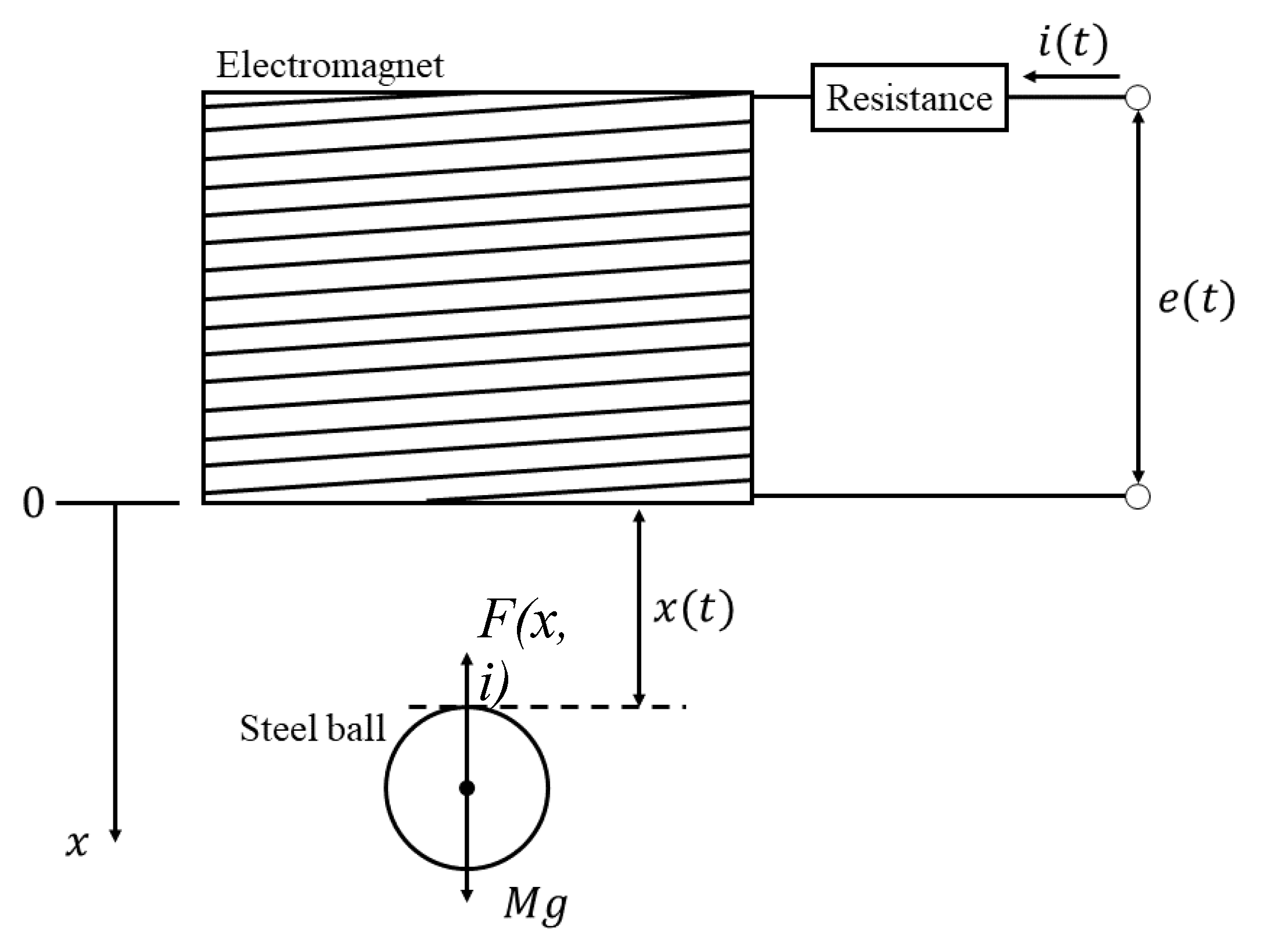
Figure 2.
Block diagram of an integer-order servo LQR control system with an integer-order state-observer.
Figure 2.
Block diagram of an integer-order servo LQR control system with an integer-order state-observer.
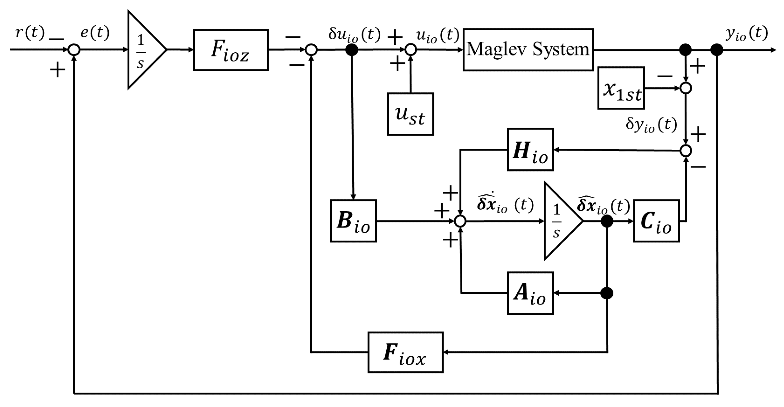
Figure 3.
Block diagram of a fractional order servo LQR control system with a fractional order state-observer.
Figure 3.
Block diagram of a fractional order servo LQR control system with a fractional order state-observer.
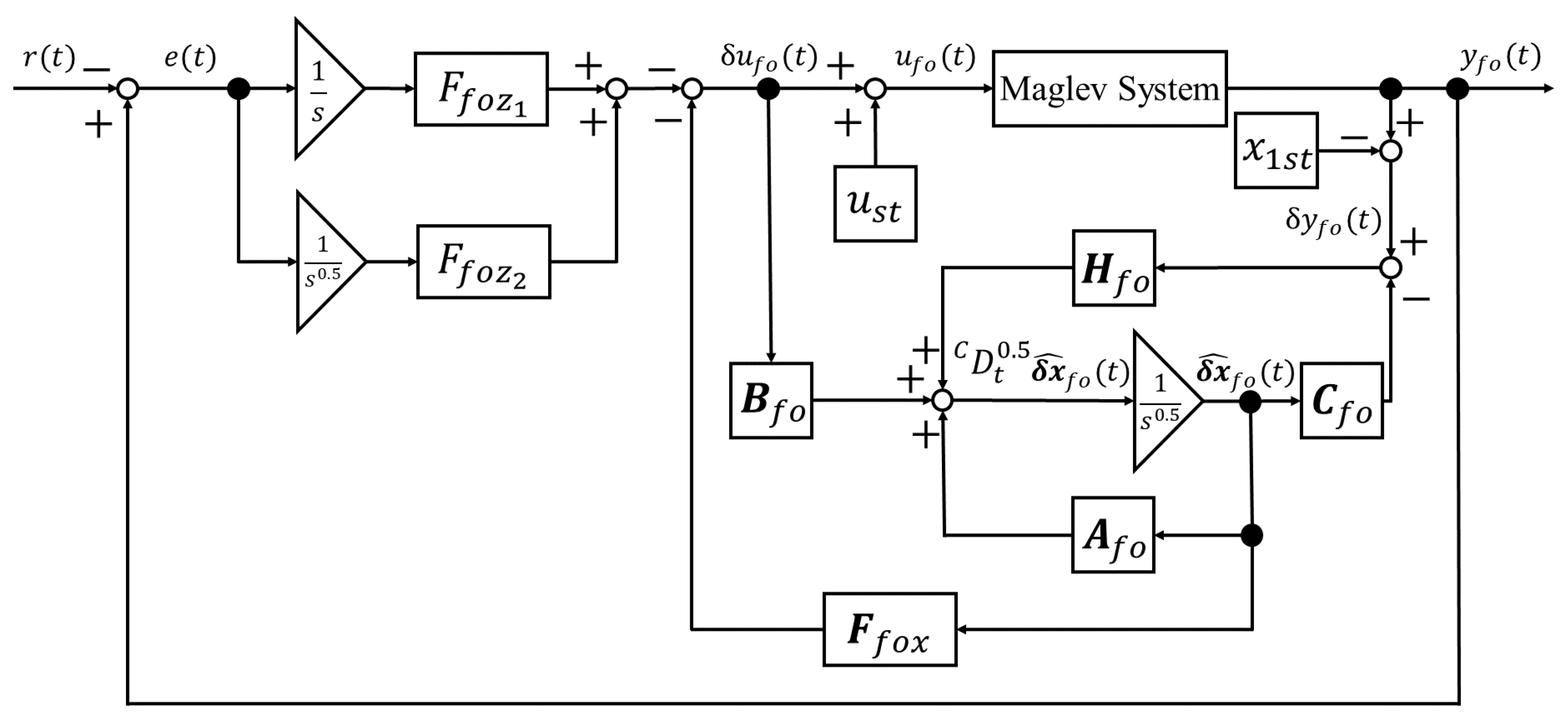
Figure 4.
Photograph of an attractive-force type magnetic levitation system.
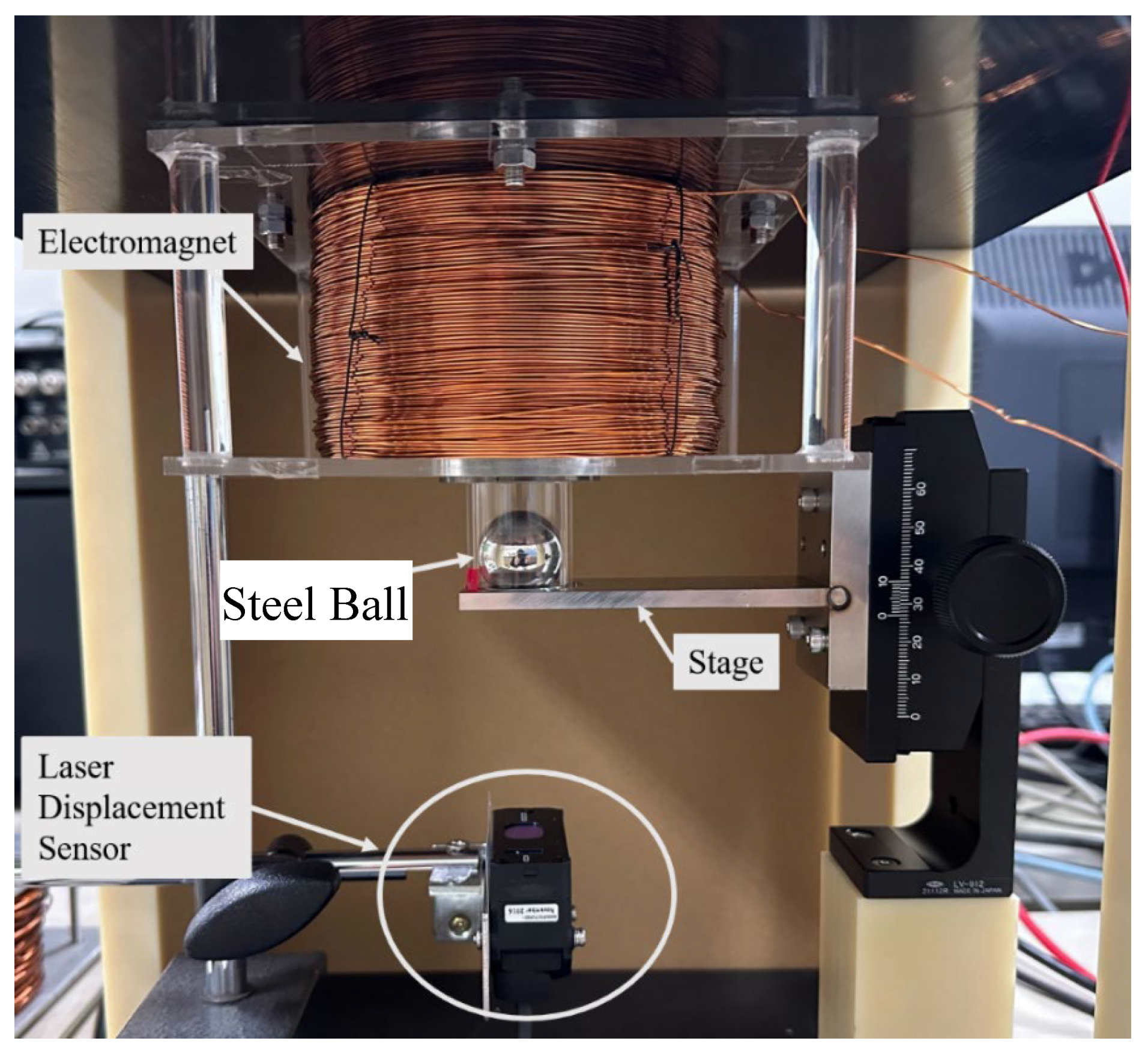
Figure 5.
Model diagram of a current-controlled attractive-force type magnetic levitation system.
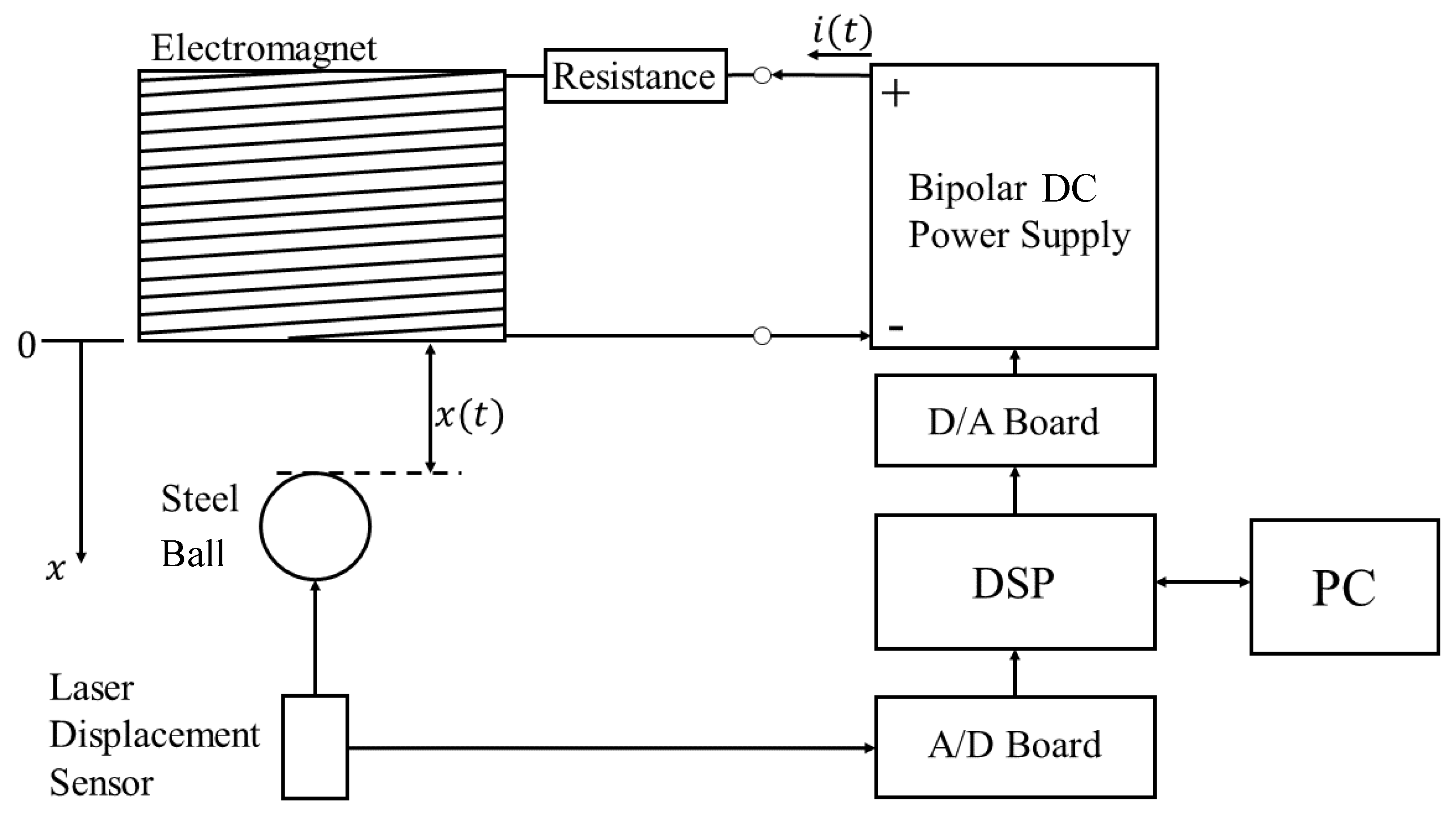
Figure 6.
Simulation I.
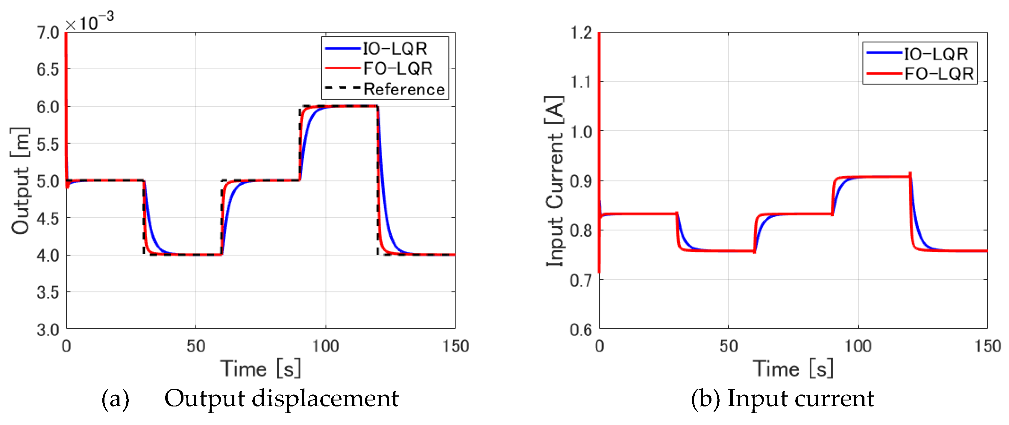
Figure 7.
Enlargements of outputs in Figure 6(a).
Figure 7.
Enlargements of outputs in Figure 6(a).
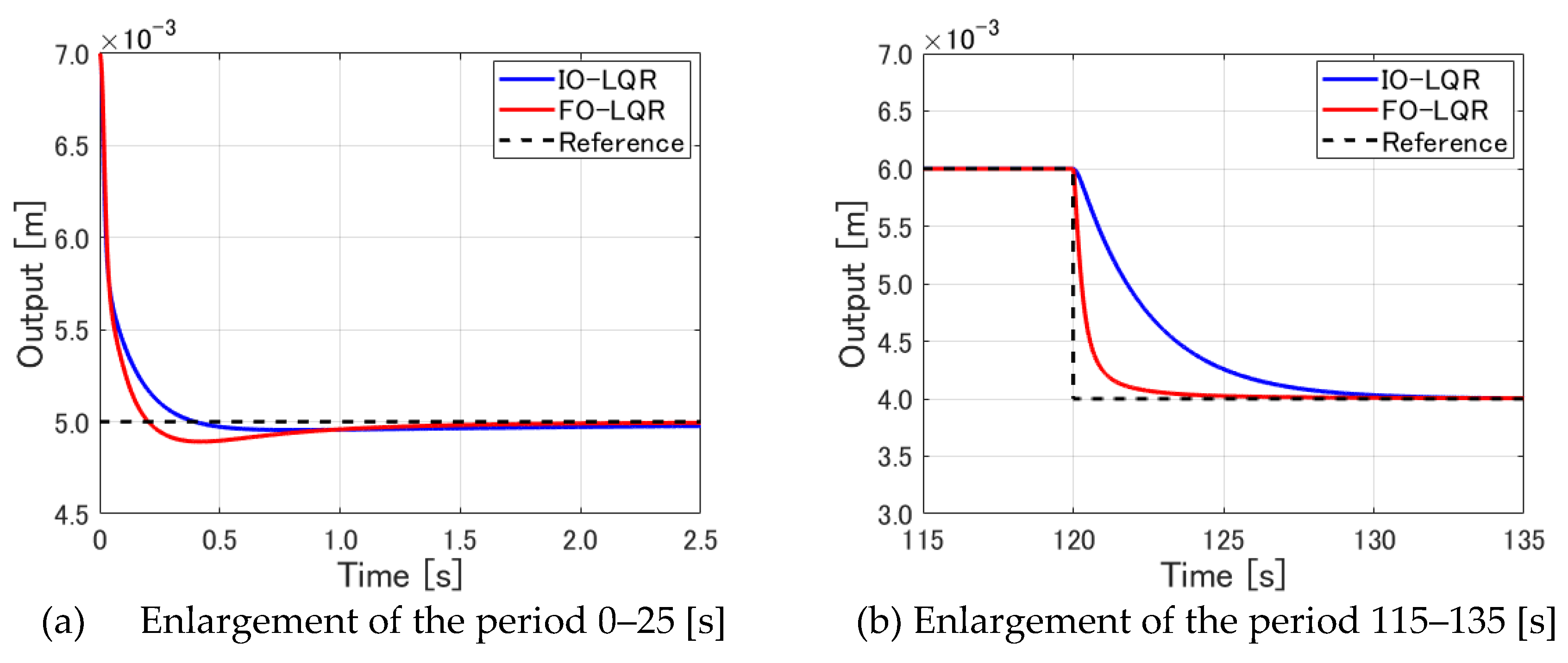
Figure 8.
Simulation II.
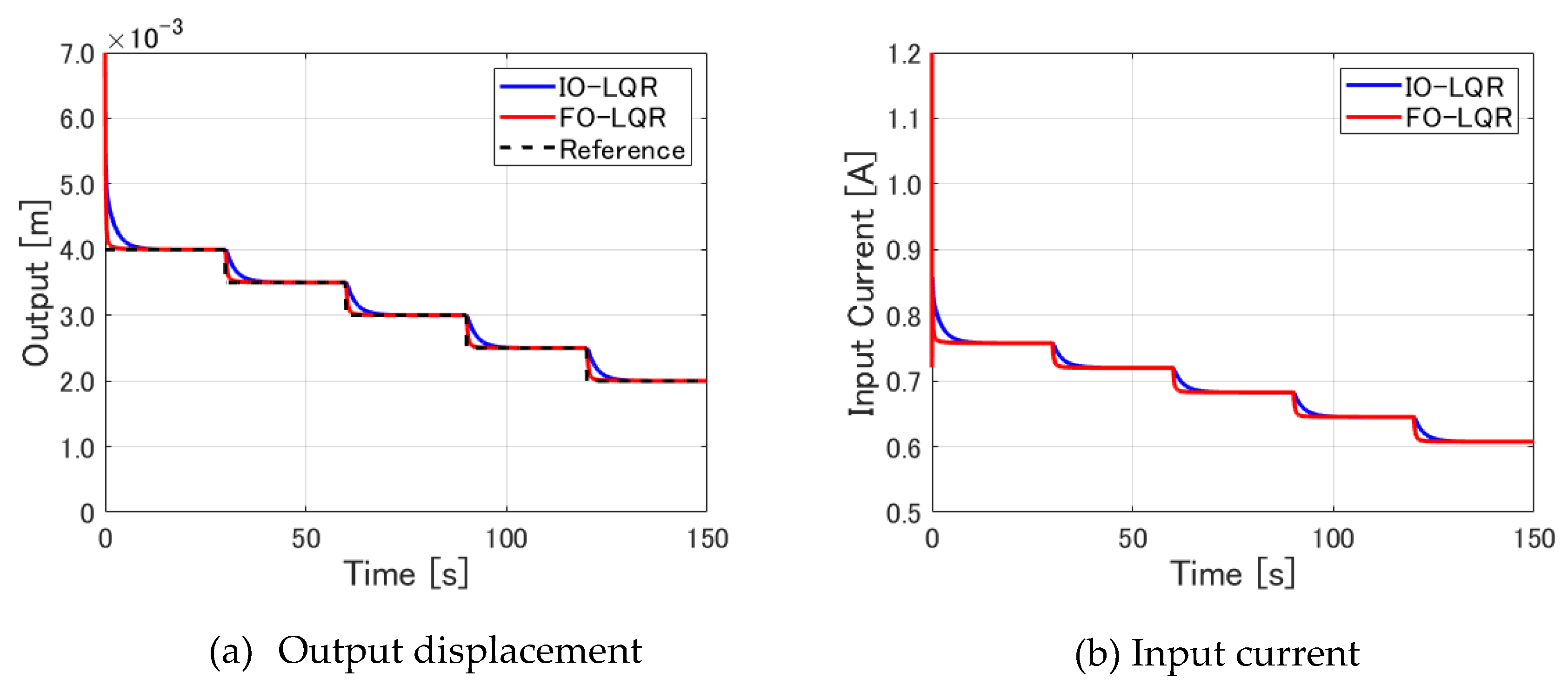
Figure 9.
Enlarged views of outputs in Figure 8(a).
Figure 9.
Enlarged views of outputs in Figure 8(a).
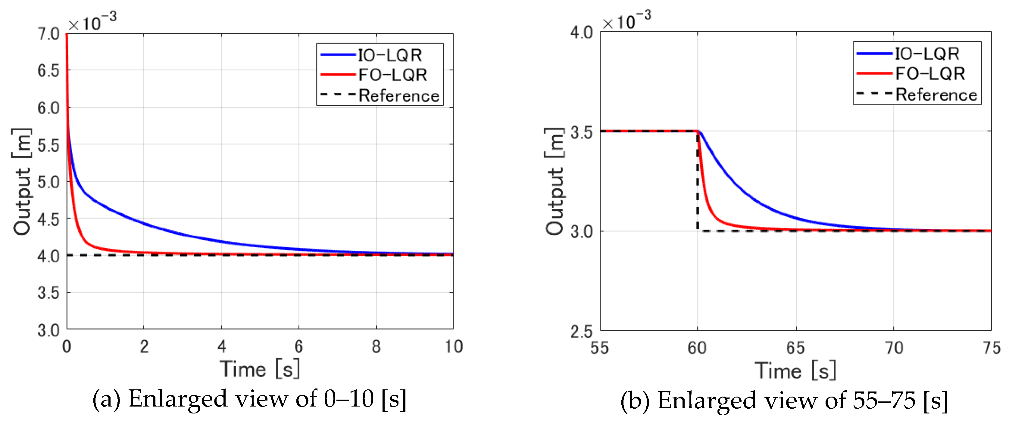
Figure 10.
Experiment I (IO-LQR control).
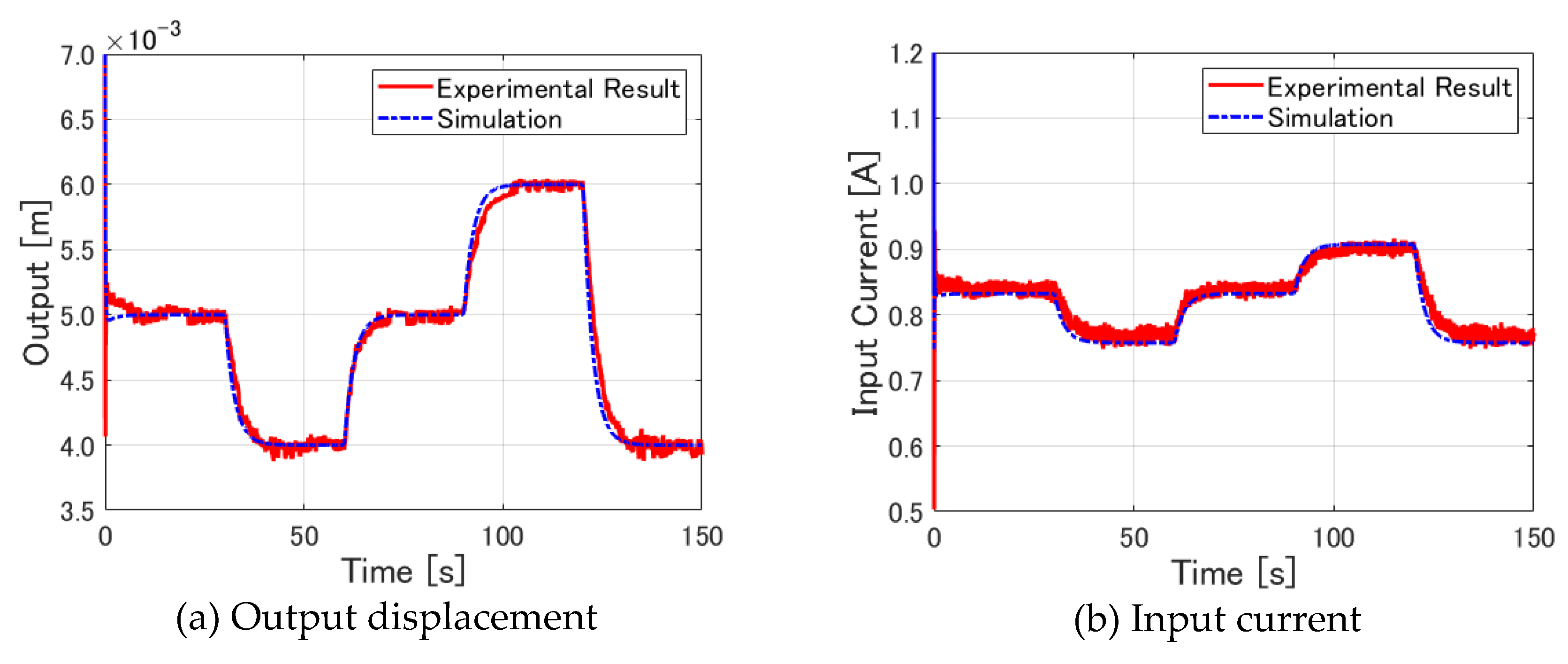
Figure 11.
Magnified views of output and input current in Figure 10.
Figure 11.
Magnified views of output and input current in Figure 10.
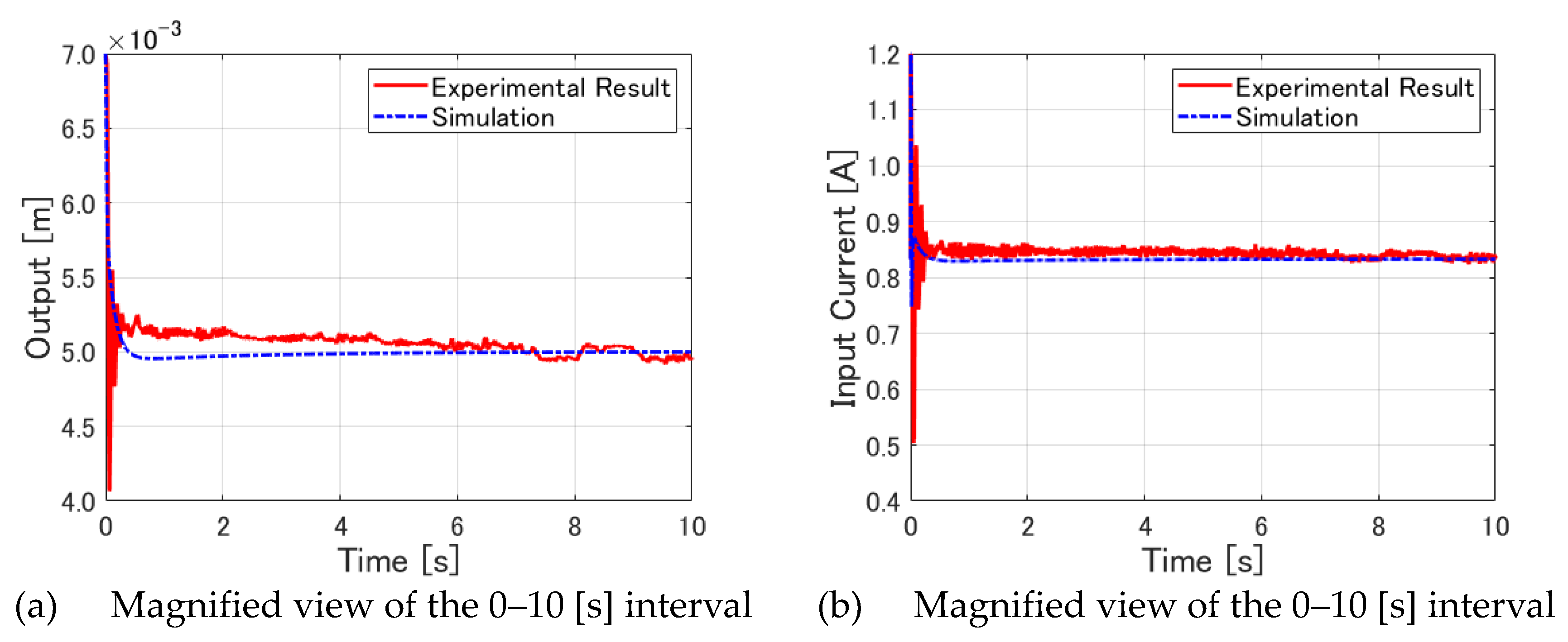
Figure 12.
Close-ups of output and input current in Figure 10.
Figure 12.
Close-ups of output and input current in Figure 10.
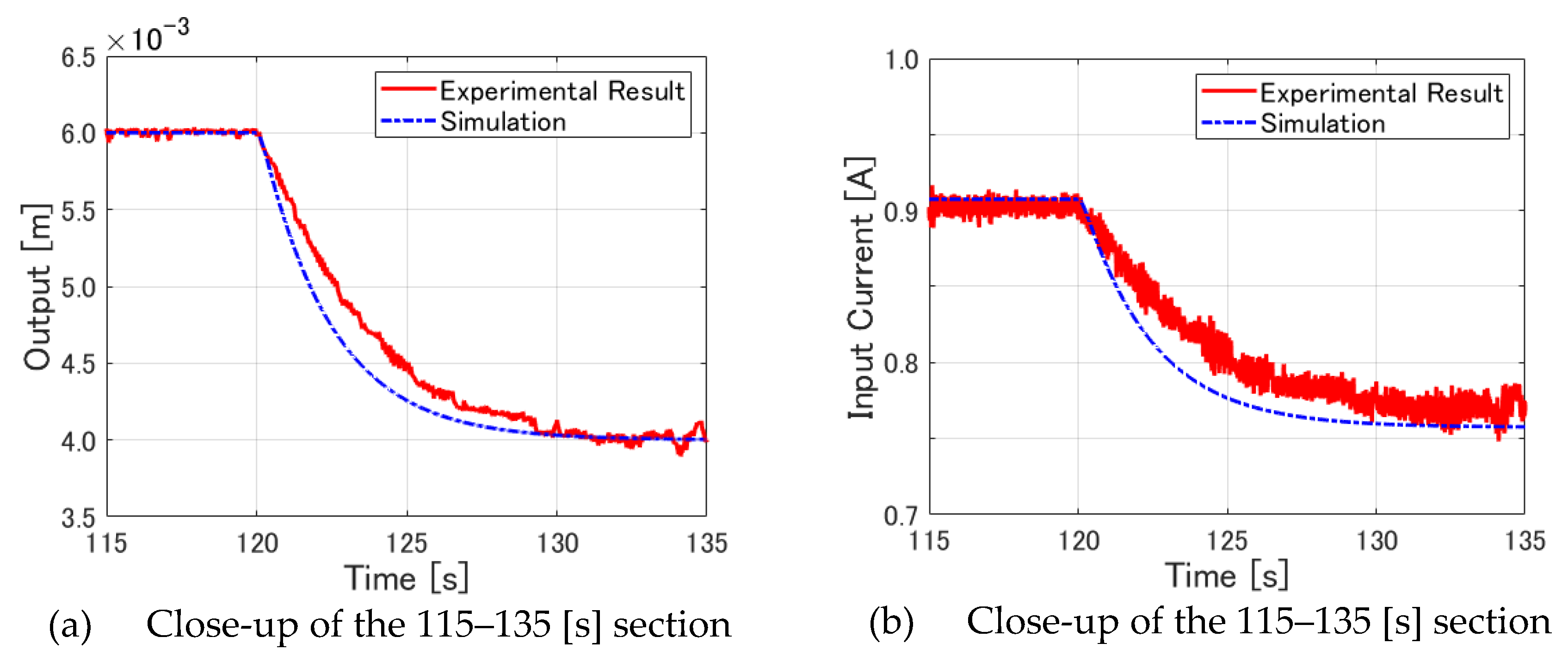
Figure 13.
Experiment II (IO-LQR control).

Figure 14.
Enlarged views of outputs in Figure 13(a).
Figure 14.
Enlarged views of outputs in Figure 13(a).

Figure 15.
Enlarged images of output and input current in Figure 13.
Figure 15.
Enlarged images of output and input current in Figure 13.
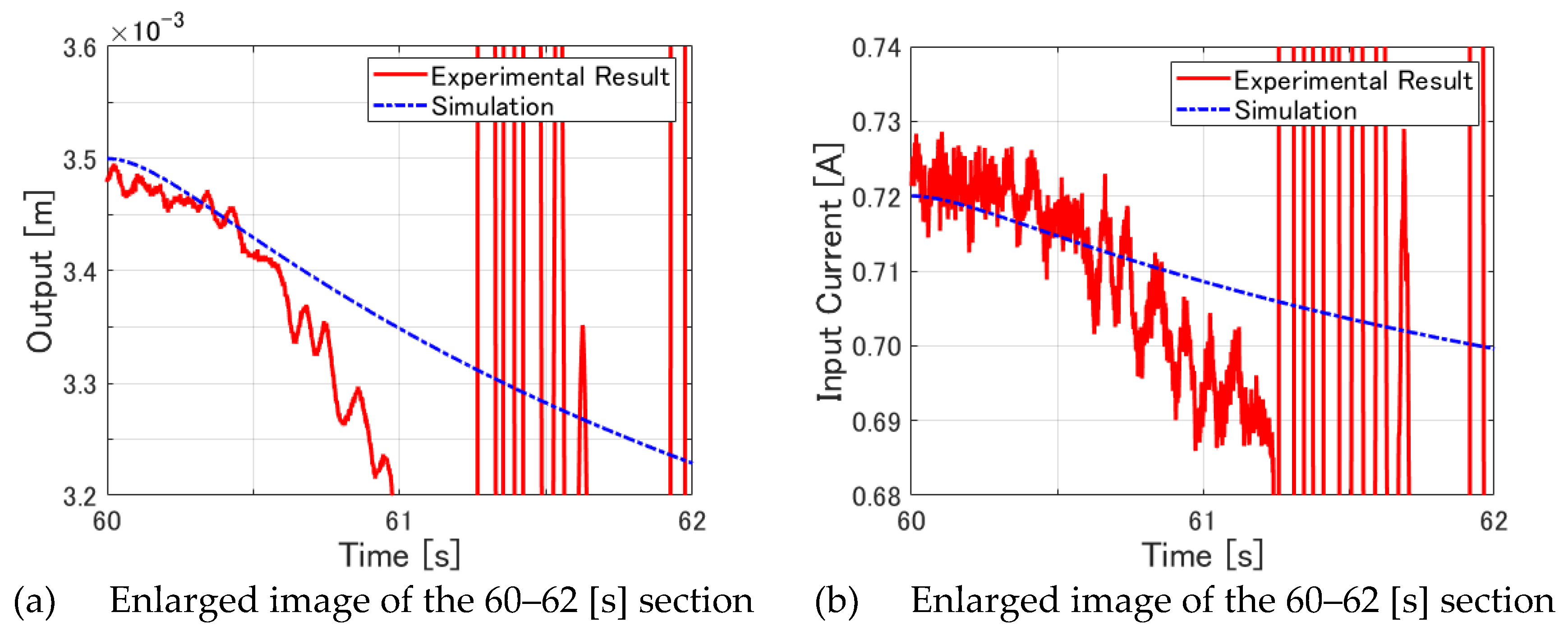
Figure 16.
Experiment I (FO-LQR control).

Figure 17.
Enlarged images of output and input current in Figure 16.
Figure 17.
Enlarged images of output and input current in Figure 16.
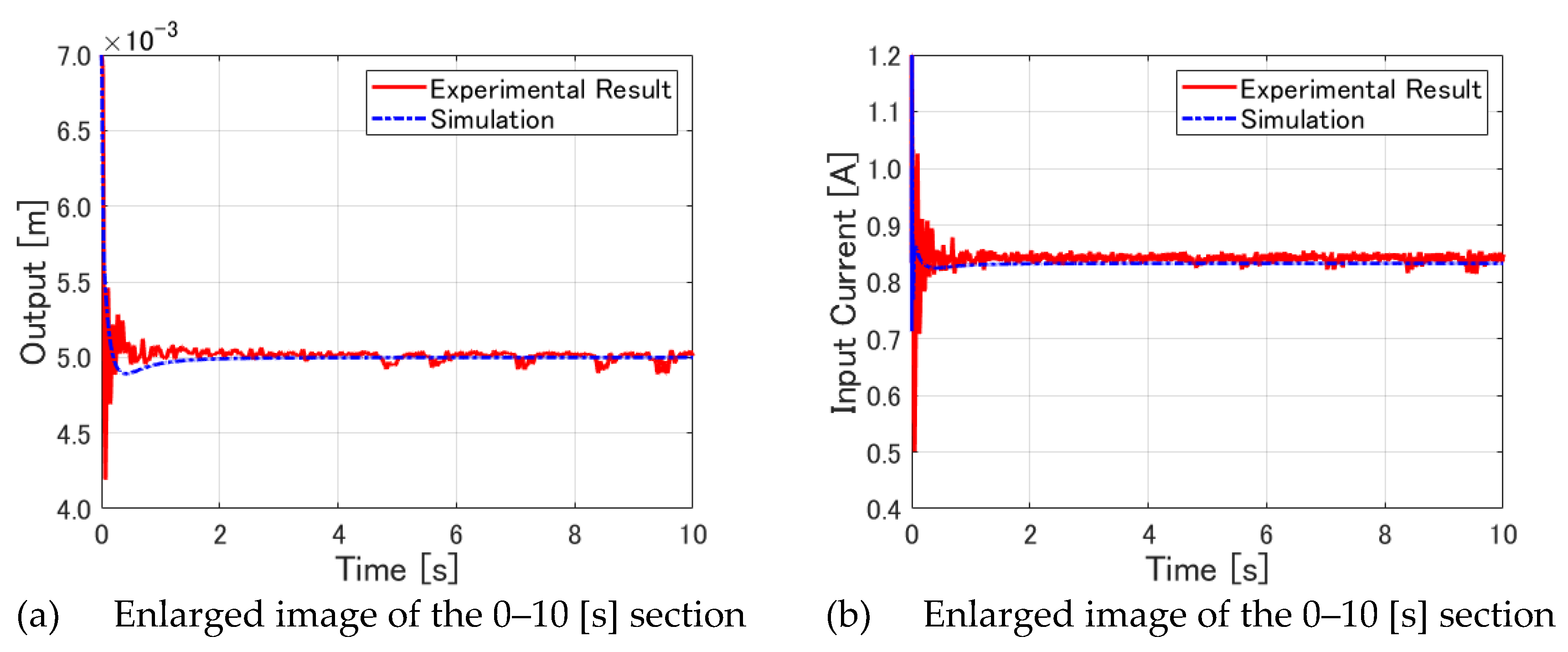
Figure 18.
Zoomed-in views of output and input current in Figure 16.
Figure 18.
Zoomed-in views of output and input current in Figure 16.
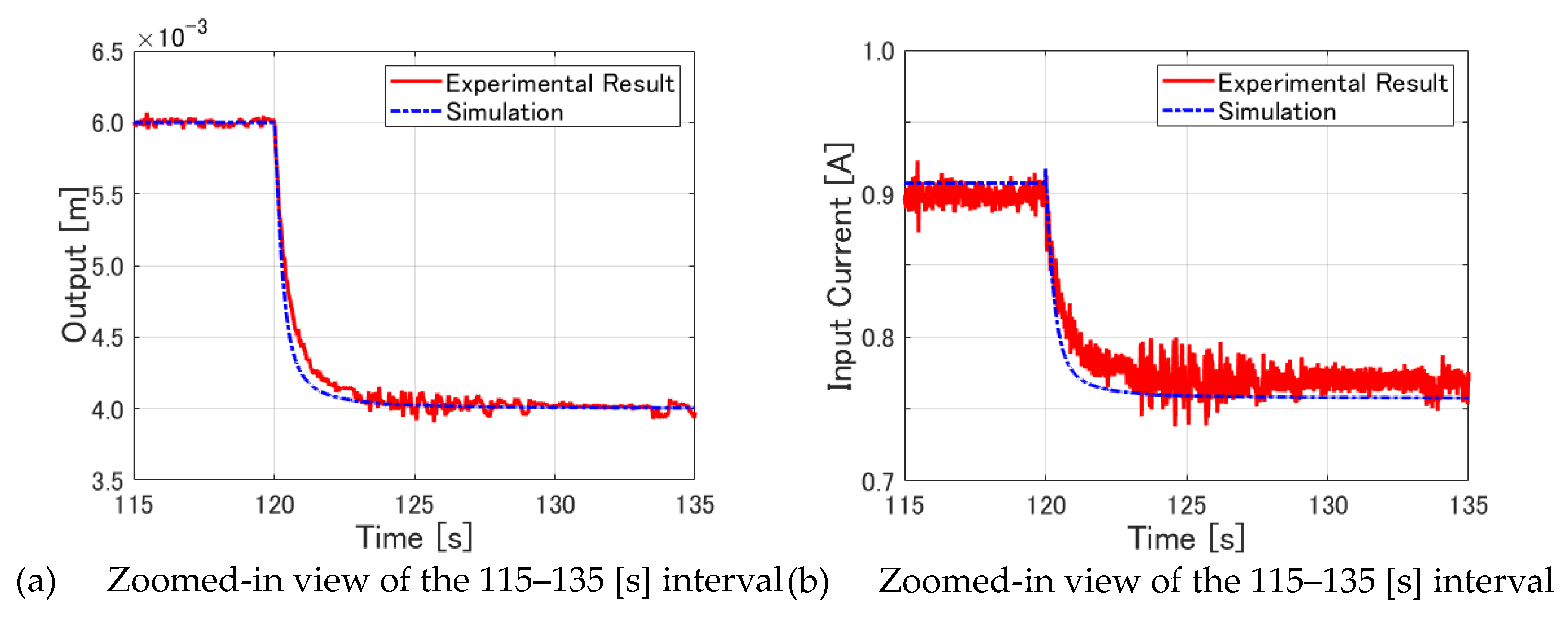
Figure 19.
Experiment II (FO-LQR control).
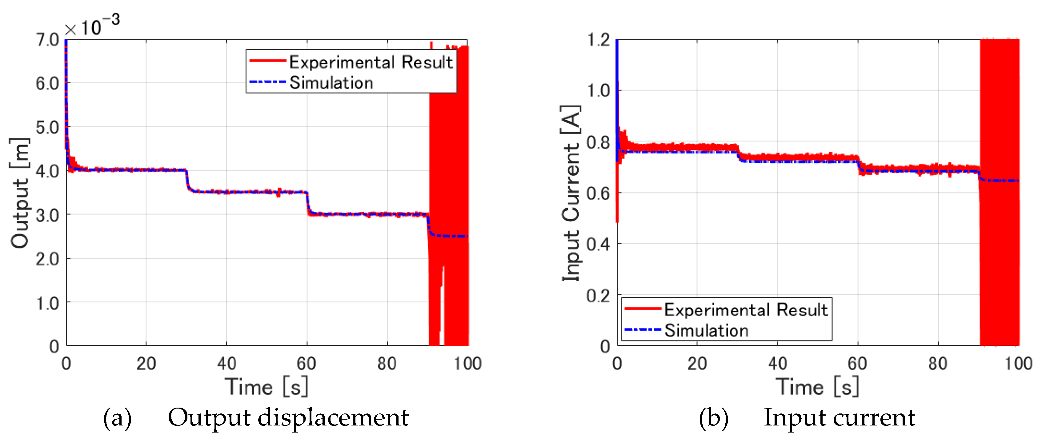
Figure 20.
Enlarged views of outputs in Figure 19(a).
Figure 20.
Enlarged views of outputs in Figure 19(a).
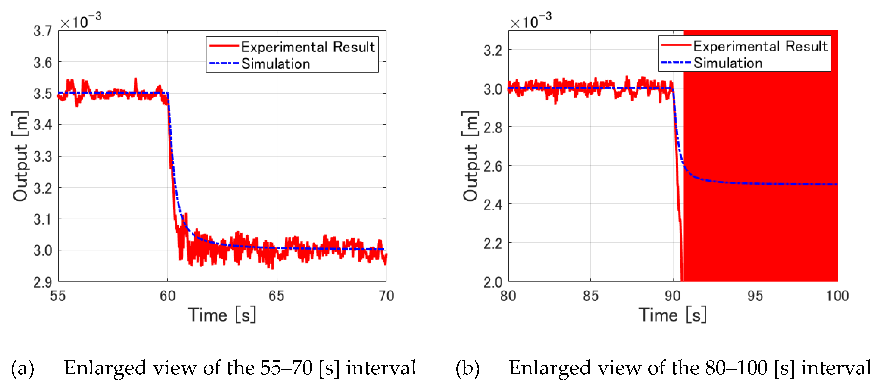
Figure 21.
Comparisons between IO and FO LQRs in Experiment I.
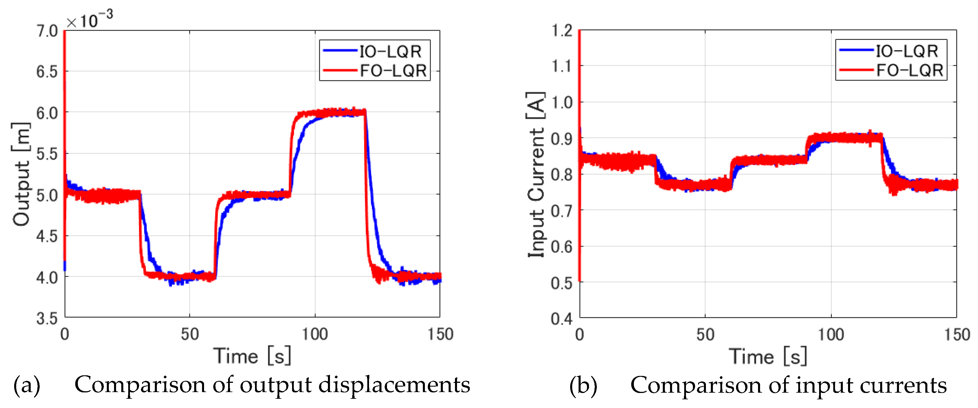
Figure 22.
Magnified images of output and input current in Figure 21.
Figure 22.
Magnified images of output and input current in Figure 21.


Figure 23.
Each input component for integer-order servo LQR control.
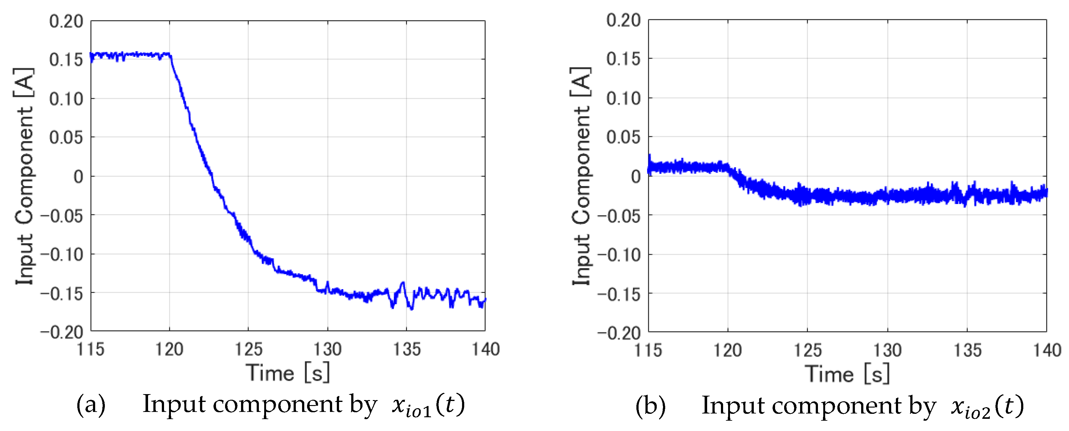
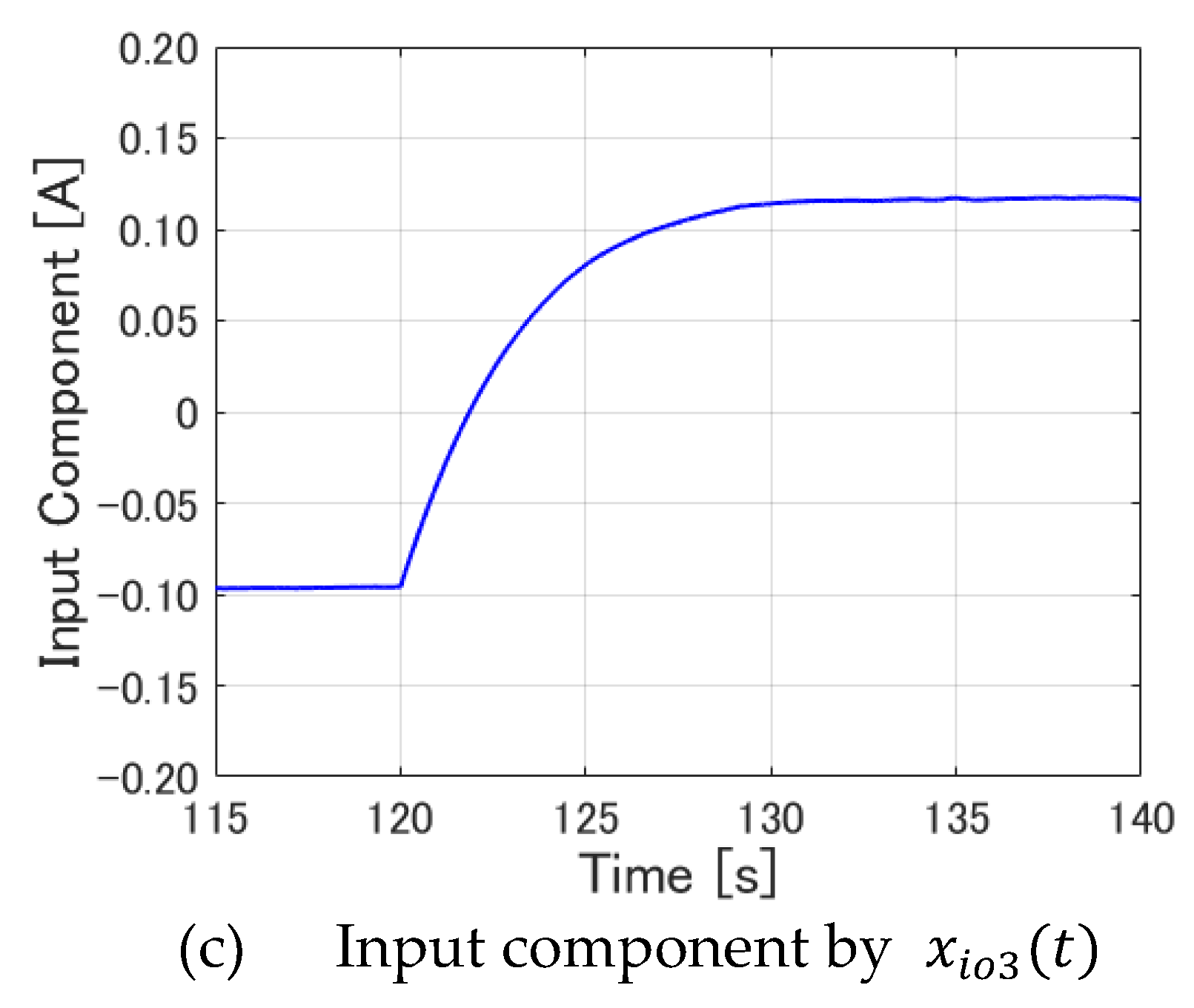
Figure 24.
Each input component for fractional order servo LQR control.
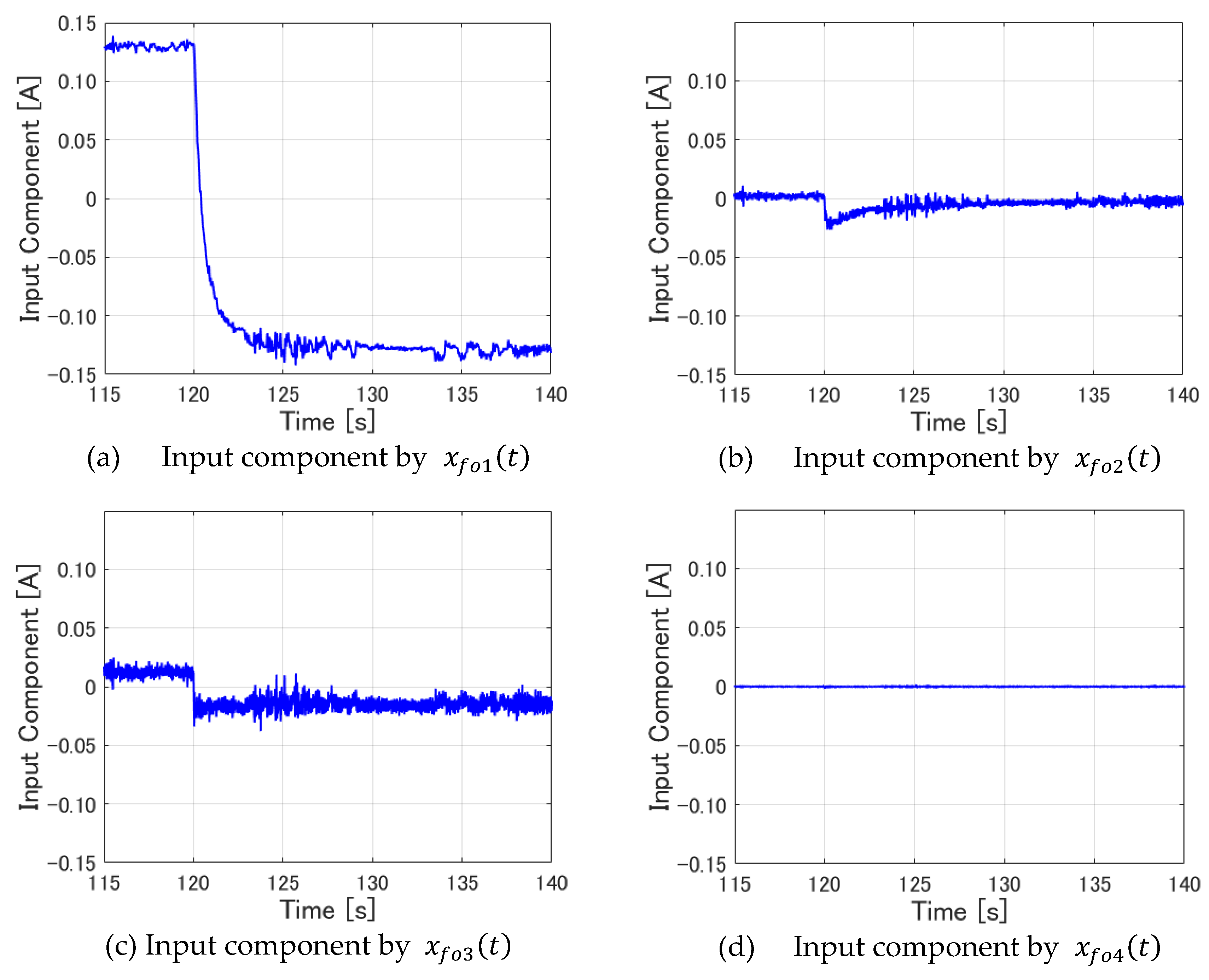
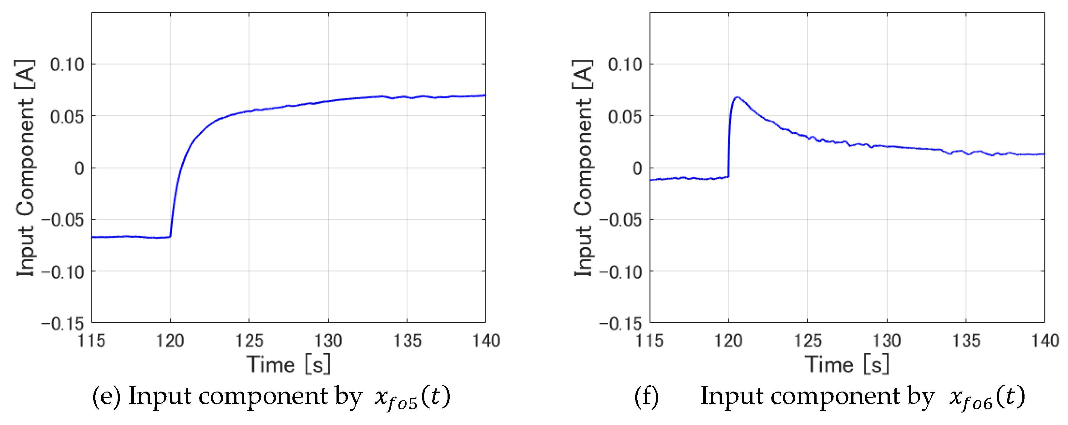

Table 1.
Physical parameters of the magnetic levitation system.
| Symbol | Description | Value |
|---|---|---|
| Mass of the steel ball | ||
| Coil coefficient | ||
| Inductance found by leakage flux | ||
| Distance found by relative permeability | ||
| Resistance of the whole circuit | ||
| Gravitational acceleration | ||
| Equilibrium displacement |
Simulations described in this chapter are performed using this experiment setup.
Disclaimer/Publisher’s Note: The statements, opinions and data contained in all publications are solely those of the individual author(s) and contributor(s) and not of MDPI and/or the editor(s). MDPI and/or the editor(s) disclaim responsibility for any injury to people or property resulting from any ideas, methods, instructions or products referred to in the content. |
© 2024 by the authors. Licensee MDPI, Basel, Switzerland. This article is an open access article distributed under the terms and conditions of the Creative Commons Attribution (CC BY) license (http://creativecommons.org/licenses/by/4.0/).
Copyright: This open access article is published under a Creative Commons CC BY 4.0 license, which permit the free download, distribution, and reuse, provided that the author and preprint are cited in any reuse.


