Submitted:
17 June 2024
Posted:
27 June 2024
You are already at the latest version
Abstract
Keywords:
1. Introduction
1.1. Review of Related Works
2. Materials and Methods
2.1. Dataset Details
2.2. Need for Feature Extraction (FE)
2.2.1. Short-Time Fourier Transform (STFT)
2.2.2. Ridge Regression (RR)
- represents the locally estimated coefficient vector for a specific data subset.
- denotes the design matrix for the data subset.
- represents the outcome vector for the data subset.
- is the regularization parameter for the local ridge regression on the i-th subset.
- I is the identity matrix with the same dimension as .
- represents the final combined coefficient vector obtained from all data subsets.
- represents the weight assigned to the local estimator from the data subset.
- represents the locally estimated coefficient vector for the data subset (as defined earlier).
2.2.3. Pearson Correlation Coefficient (PCC)
3. Feature Selection Method
3.1. Bald Eagle Search Optimization (BESO)
3.2. Red Deer Optimization (RDO)
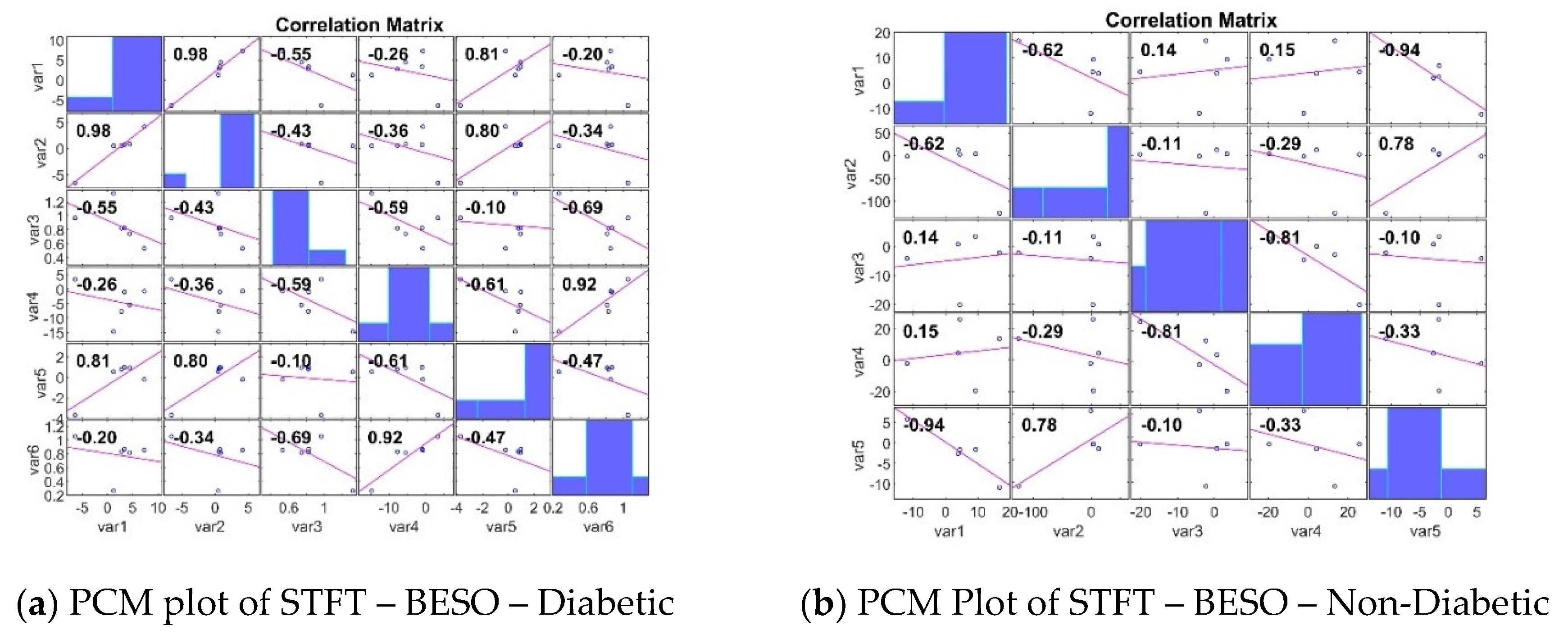
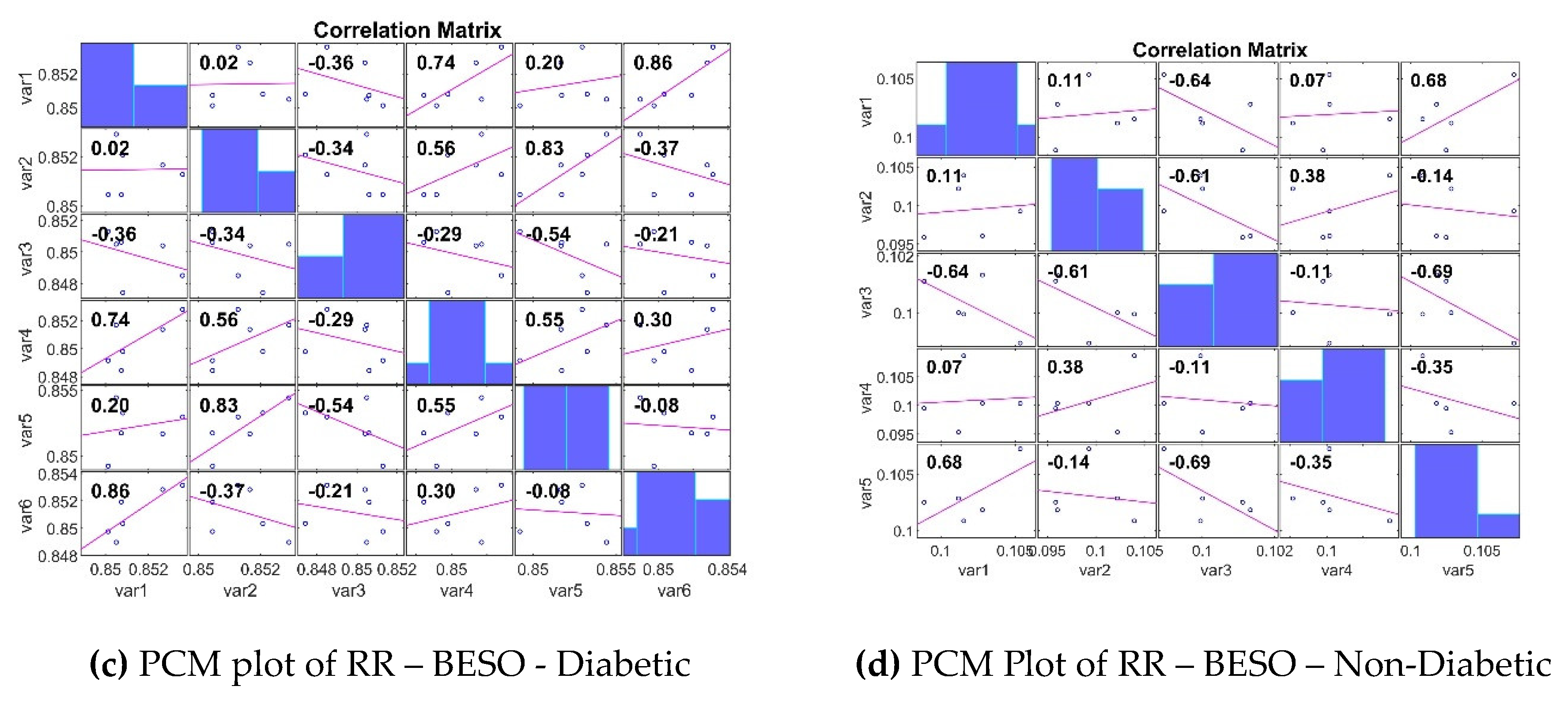
3.3. Analyzing the Impact of Feature Extraction Methods Using Statistical Measures
4. Classifiers
4.1. Non-linear Regression
4.2. Linear Regression
4.3. Gaussian Mixture Model
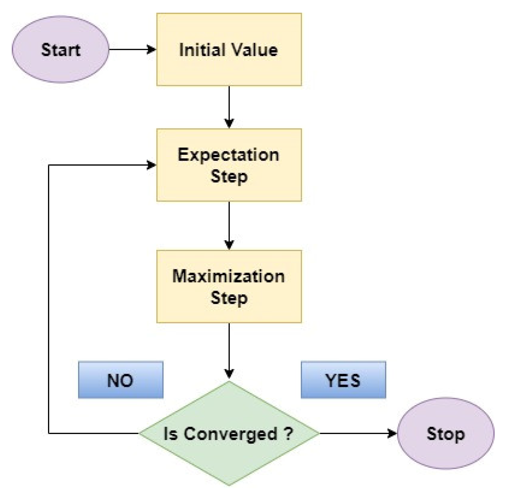
4.4. Expectation Maximum
- Expectation Step: In this initial step, the EM algorithm estimates the missing information, or hidden factors based on the currently available data and the current model parameters.
- Maximization Step: With the estimated missing values in place, the EM algorithm then refines the model parameters by considering the newly completed data.
4.5. Logistic Regression
4.6. Softmax Discriminant Classifier
4.7. Support Vector Machine (Radial Basis Function)
4.8. Selection of Classifiers Parameters through Training and Testing
5. Classifiers Training and Testing
5.1. Selection of Targets
6. Outcomes and Findings
6.1. Computational Complexity
6.2. Limitations
6.3. Conclusions and Future Work
References
- Saeedi, P., Petersohn, I., Salpea, P., Malanda, B., Karuranga, S., Unwin, N., ... & IDF Diabetes Atlas Committee. (2019). Global and regional diabetes prevalence estimates for 2019 and projections for 2030 and 2045: Results from the International Diabetes Federation Diabetes Atlas. Diabetes research and clinical practice, 157, 107843.
- Mohan, V., Sudha, V., Shobana, S., Gayathri, R., & Krishnaswamy, K. (2023). Are unhealthy diets contributing to the rapid rise of type 2 diabetes in India?. The Journal of Nutrition, 153(4), 940-948.
- Oberoi, S., & Kansra, P. (2020). Economic menace of diabetes in India: a systematic review. International journal of diabetes in developing countries, 40, 464-475.
- Chellappan, D., & Rajaguru, H. (2023). Detection of Diabetes through Microarray Genes with Enhancement of Classifiers Performance. Diagnostics, 13(16), 2654.
- Gowthami, S., Reddy, R. V. S., & Ahmed, M. R. (2024). Exploring the effectiveness of machine learning algorithms for early detection of Type-2 Diabetes Mellitus. Measurement: Sensors, 31, 100983.c.
- Tasin, I., Nabil, T. U., Islam, S., & Khan, R. (2023). Diabetes prediction using machine learning and explainable AI techniques. Healthcare technology letters, 10(1-2), 1-10.
- Frasca, M., La Torre, D., Pravettoni, G., & Cutica, I. (2024). Explainable and interpretable artificial intelligence in medicine: a systematic bibliometric review. Discover Artificial Intelligence, 4(1), 15.
- Chaddad, A., Peng, J., Xu, J., & Bouridane, A. (2023). Survey of explainable AI techniques in healthcare. Sensors, 23(2), 634.
- Hussain, F., Hussain, R., & Hossain, E. (2021). Explainable artificial intelligence (XAI): An engineering perspective. arXiv preprint arXiv:2101.03613. arXiv:2101.03613.
- Markus, A. F., Kors, J. A., & Rijnbeek, P. R. (2021). The role of explainability in creating trustworthy artificial intelligence for health care: a comprehensive survey of the terminology, design choices, and evaluation strategies. Journal of biomedical informatics, 113, 103655.
- Prajapati, S., Das, H., & Gourisaria, M. K. (2023). Feature selection using differential evolution for microarray data classification. Discover Internet of Things, 3(1), 12.
- Alsattar, H. A., Zaidan, A. A., & Zaidan, B. B. (2020). Novel meta-heuristic bald eagle search optimisation algorithm. Artificial Intelligence Review, 53, 2237-2264.
- Hilal, A. M., Alrowais, F., Al-Wesabi, F. N., & Marzouk, R. (2023). Red Deer Optimization with Artificial Intelligence Enabled Image Captioning System for Visually Impaired People. Computer Systems Science & Engineering, 46(2).
- Horng, J. T., Wu, L. C., Liu, B. J., Kuo, J. L., Kuo, W. H., & Zhang, J. J. (2009). An expert system to classify microarray gene expression data using gene selection by decision tree. Expert Systems with Applications, 36(5), 9072-9081.
- Shaik, B. S., Naganjaneyulu, G. V. S. S. K. R., Chandrasheker, T., & Narasimhadhan, A. V. (2015). A method for QRS delineation based on STFT using adaptive threshold. Procedia Computer Science, 54, 646-653.
- Bar, N., Nikparvar, B., Jayavelu, N. D., & Roessler, F. K. (2022). Constrained Fourier estimation of short-term time-series gene expression data reduces noise and improves clustering and gene regulatory network predictions. BMC bioinformatics, 23(1), 330.
- Imani, M., & Ghassemian, H. (2015). Ridge regression-based feature extraction for hyperspectral data. International Journal of Remote Sensing, 36(6), 1728-1742.
- Paul, S., & Drineas, P. (2016). Feature selection for ridge regression with provable guarantees. Neural computation, 28(4), 716-742.
- Prabhakar, S. K., Rajaguru, H., Ryu, S., Jeong, I. C., & Won, D. O. (2022). A holistic strategy for classification of sleep stages with EEG. Sensors, 22(9), 3557.
- Mehta, P., Bukov, M., Wang, C. H., Day, A. G., Richardson, C., Fisher, C. K., & Schwab, D. J. (2019). A high-bias, low-variance introduction to machine learning for physicists. Physics reports, 810, 1-124.
- Li, G., Zhang, A., Zhang, Q., Wu, D., & Zhan, C. (2022). Pearson correlation coefficient-based performance enhancement of broad learning system for stock price prediction. IEEE Transactions on Circuits and Systems II: Express Briefs, 69(5), 2413-2417.
- Mu, Y., Liu, X., & Wang, L. (2018). A Pearson’s correlation coefficient-based decision tree and its parallel implementation. Information Sciences, 435, 40-58.
- Grace Elizabeth Rani, T. G., & Jayalalitha, G. (2016). Complex patterns in financial time series through Higuchi’s fractal dimension. Fractals, 24(04), 1650048.
- Rehan, I., Rehan, K., Sultana, S., & Rehman, M. U. (2024). Fingernail Diagnostics: Advancing type II diabetes detection using machine learning algorithms and laser spectroscopy. Microchemical Journal, 110762.
- Alsattar, H. A., Zaidan, A. A., & Zaidan, B. B. (2020). Novel meta-heuristic bald eagle search optimisation algorithm. Artificial Intelligence Review, 53, 2237-2264.
- Kwakye, B. D., Li, Y., Mohamed, H. H., Baidoo, E., & Asenso, T. Q. (2024). Particle guided metaheuristic algorithm for global optimization and feature selection problems. Expert Systems with Applications, 248, 123362.
- Wang, J., Ouyang, H., Zhang, C., Li, S., & Xiang, J. (2023). A novel intelligent global harmony search algorithm based on improved search stability strategy. Scientific Reports, 13(1), 7705.
- Fard AF, Hajiaghaei-Keshteli M. Red Deer Algorithm (RDA); a new optimization algorithm inspired by Red Deers’ mating. In: International conference on industrial engineering. IEEE; 2016, p. 331–42, 12. (2016).
- Fathollahi-Fard, et al. Red deer algorithm (RDA): a new nature-inspired meta-heuristic. Soft Comput 2020;24.19:14637–65, (2020).
- Bektaş, Y., & Karaca, H. (2022). Red deer algorithm based selective harmonic elimination for renewable energy application with unequal DC sources. Energy Reports, 8, 588-596.
- Anonymous. Kumar, A. P., & Valsala, P. (2013). Feature Selection for high Dimensional DNA Microarray data using hybrid approaches. Bioinformation, 9(16), 824.
- Zhang, G.; Allaire, D.; Cagan, J. Reducing the Search Space for Global Minimum: A Focused Regions Identification Method for Least Squares Parameter Estimation in Nonlinear Models. J. Comput. Inf. Sci. Eng. 2023, 23, 021006. [Google Scholar] [CrossRef]
- Draper, N.R.; Smith, H. Applied Regression Analysis; John Wiley & Sons: Hoboken, NJ, USA, 1998; Volume 326. [Google Scholar]
- Zhang, G.; Allaire, D.; Cagan, J. Reducing the Search Space for Global Minimum: A Focused Regions Identification Method for Least Squares Parameter Estimation in Nonlinear Models. J. Comput. Inf. Sci. Eng. 2023, 23, 021006. [Google Scholar] [CrossRef]
- Prabhakar, S.K.; Rajaguru, H.; Lee, S.-W. A comprehensive analysis of alcoholic EEG signals with detrend fluctuation analysis and post classifiers. In Proceedings of the 2019 7th International Winter Conference on Brain-Computer Interface (BCI), Gangwon, Republic of Korea, 18–20 February 2019. [Google Scholar]
- Llaha, O.; Rista, A. Prediction and Detection of Diabetes using Machine Learning. In Proceedings of the 20th International Conference on Real-Time Applications in Computer Science and Information Technology (RTA-CSIT), Tirana, Albania, 21–22 May 2021; pp. 94–102. [Google Scholar]
- Hamid, I.Y. Prediction of Type 2 Diabetes through Risk Factors using Binary Logistic Regression. J. Al-Qadisiyah Comput. Sci. Math. 2020, 12, 1. [Google Scholar] [CrossRef]
- Liu, S., Zhang, X., Xu, L., & Ding, F. (2022). Expectation–maximization algorithm for bilinear systems by using the Rauch–Tung–Striebel smoother. Automatica, 142, 110365.
- Moon, T. K. (1996). The expectation-maximization algorithm. IEEE Signal processing magazine, 13(6), 47-60.
- Adiwijaya, K.; Wisesty, U.N.; Lisnawati, E.; Aditsania, A.; Kusumo, D.S. Dimensionality reduction using principal component analysis for cancer detection based on microarray data classification. J. Comput. Sci. 2018, 14, 1521–1530. [Google Scholar] [CrossRef]
- Peng, C. Y. J., Lee, K. L., & Ingersoll, G. M. (2002). An introduction to logistic regression analysis and reporting. The journal of educational research, 96(1), 3-14.
- Zang, F.; Zhang, J.S. Softmax Discriminant Classifier. In Proceedings of the 3rd International Conference on Multimedia Information Networking and Security, Shanghai, China, 4–6 November 2011; pp. 16–20. [Google Scholar]
- Yao, X.; Panaye, A.; Doucet, J.; Chen, H.; Zhang, R.; Fan, B.; Liu, M.; Hu, Z. Comparative classification study of toxicity mechanisms using support vector machines and radial basis function neural networks. Anal. Chim. Acta 2005, 535, 259–273. [Google Scholar] [CrossRef]
- Ortiz-Martínez, M., González-González, M., Martagón, A. J., Hlavinka, V., Willson, R. C., & Rito-Palomares, M. (2022). Recent developments in biomarkers for diagnosis and screening of type 2 diabetes mellitus. Current diabetes reports, 22(3), 95-115.
- Maxwell, A. E., Warner, T. A., & Guillén, L. A. (2021). Accuracy assessment in convolutional neural network-based deep learning remote sensing studies—Part 1: Literature review. Remote Sensing, 13(13), 2450.
- Maniruzzaman M, Kumar N, Abedin MM, Islam MS, Suri HS, El-Baz AS, Suri JS. Comparative approaches for classifi-cation of diabetes mellitus data: machine learning paradigm. Comput Methods Programs Biomed. 2017;152:23–34.
- Hertroijs DFL, Elissen AMJ, Brouwers MCGJ, Schaper NC, Köhler S, Popa MC, Asteriadis S, Hendriks SH, Bilo HJ, Ruwaard D, et al. A risk score including body mass index, glycated hemoglobin and triglycerides predicts future glycemic control in people with type 2 diabetes. Diabetes Obes Metab. 2017;20(3):681–8.
- Deo R, Panigrahi S. Performance assessment of machine learning based models for diabetes prediction. In: 2019 IEEE healthcare innovations and point of care technologies, (HI-POCT). 2019.
- Akula R, Nguyen N, Garibay I. Supervised machine learning based ensemble model for accurate prediction of type 2 diabetes. In: 2019 Southeast Con. 2019.
- Xie Z, Nikolayeva O, Luo J, Li D. Building risk prediction models for type 2 diabetes using machine learning techniques. Prev Chronic Dis. 2019.
- Bernardini M, Morettini M, Romeo L, Frontoni E, Burattini L. Early temporal prediction of type 2 diabetes risk condition from a general practitioner electronic health record: a multiple instance boosting approach. ArtifIntell Med. 2020;105:101847.
- Zhang L, Wang Y, Niu M, Wang C, Wang Z. Nonlaboratory based risk assessment model for type 2 diabetes mellitus screening in Chinese rural population: a joint bagging boosting model. IEEE J Biomed Health Inform. 2021;25(10):4005–16.
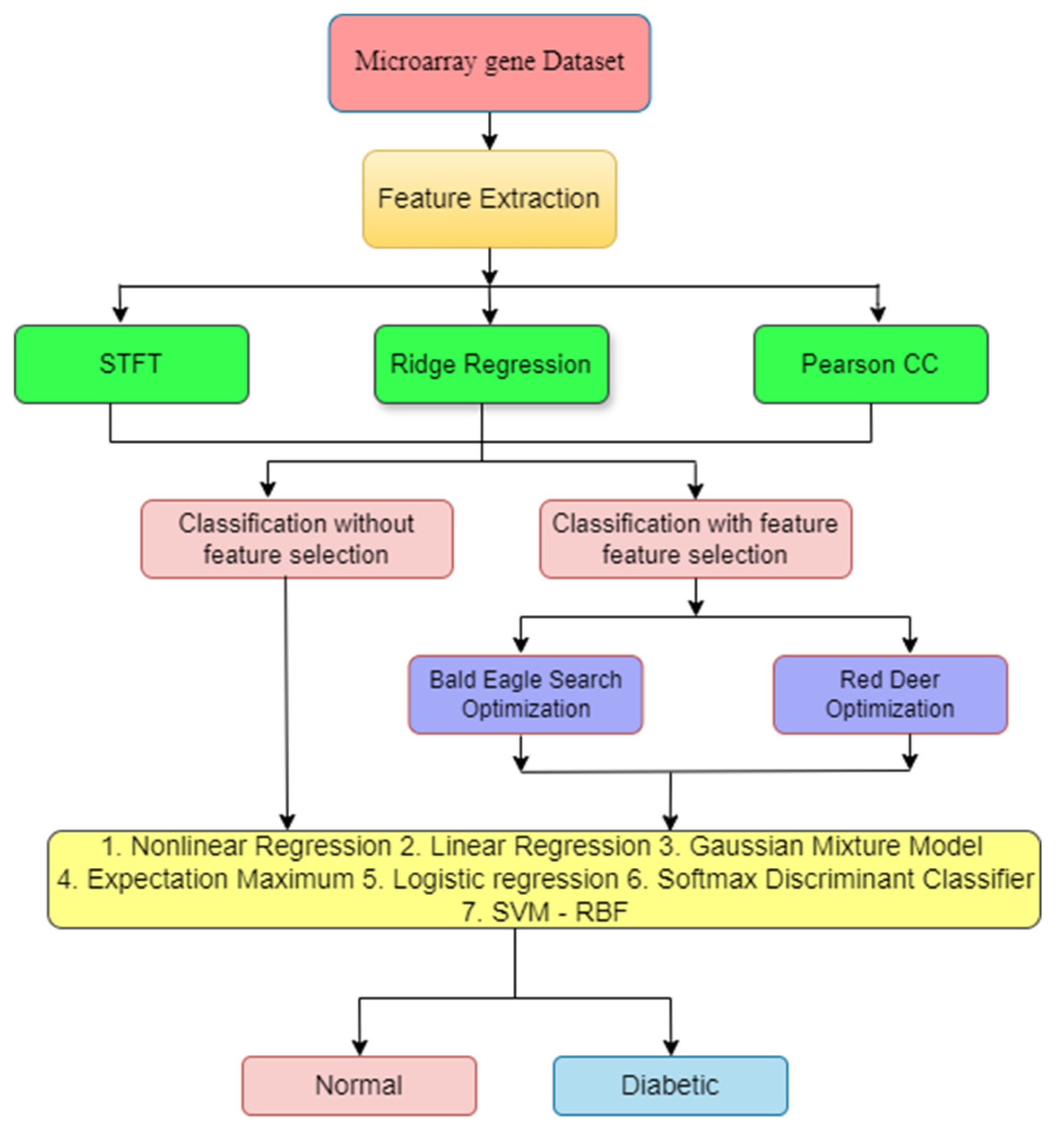
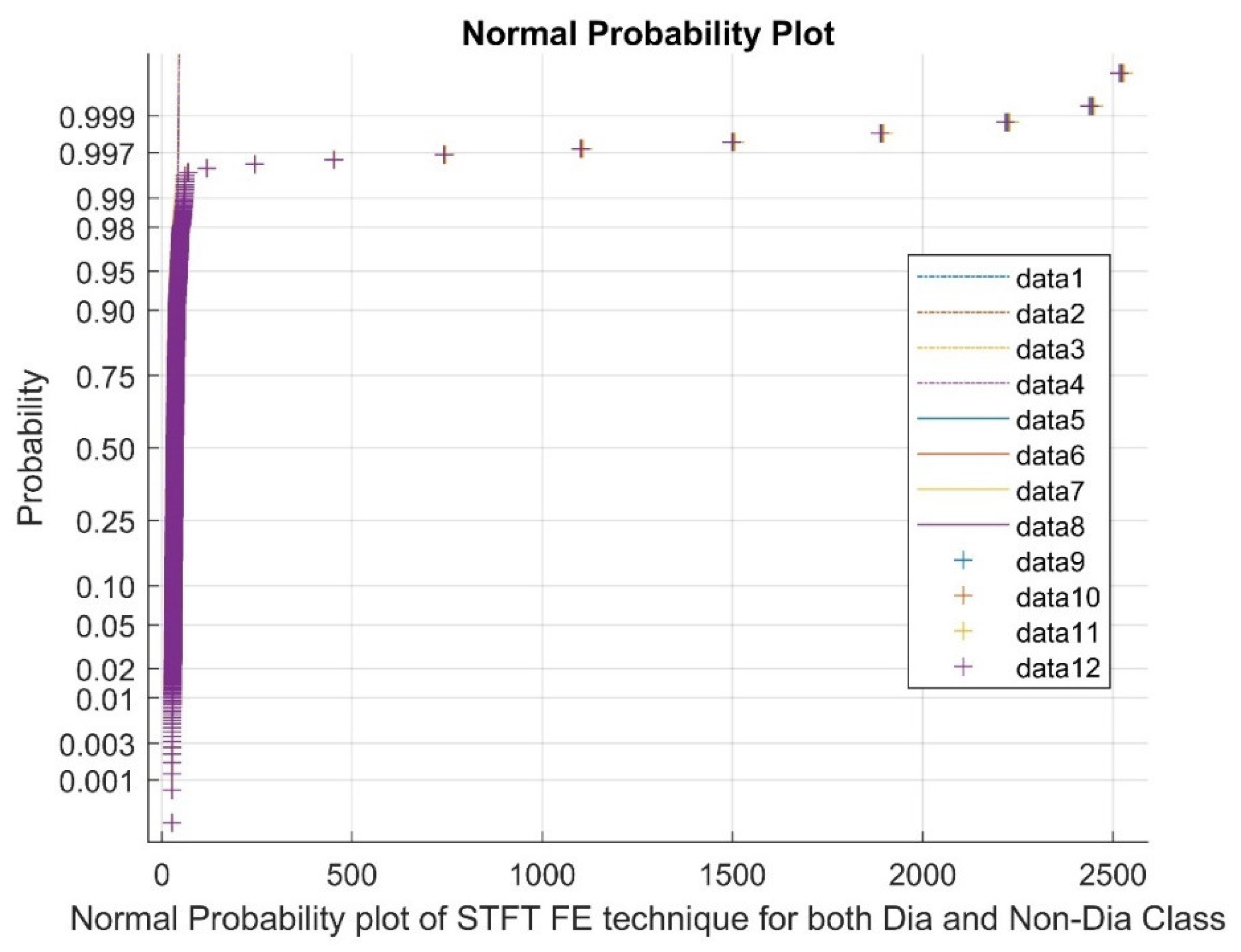
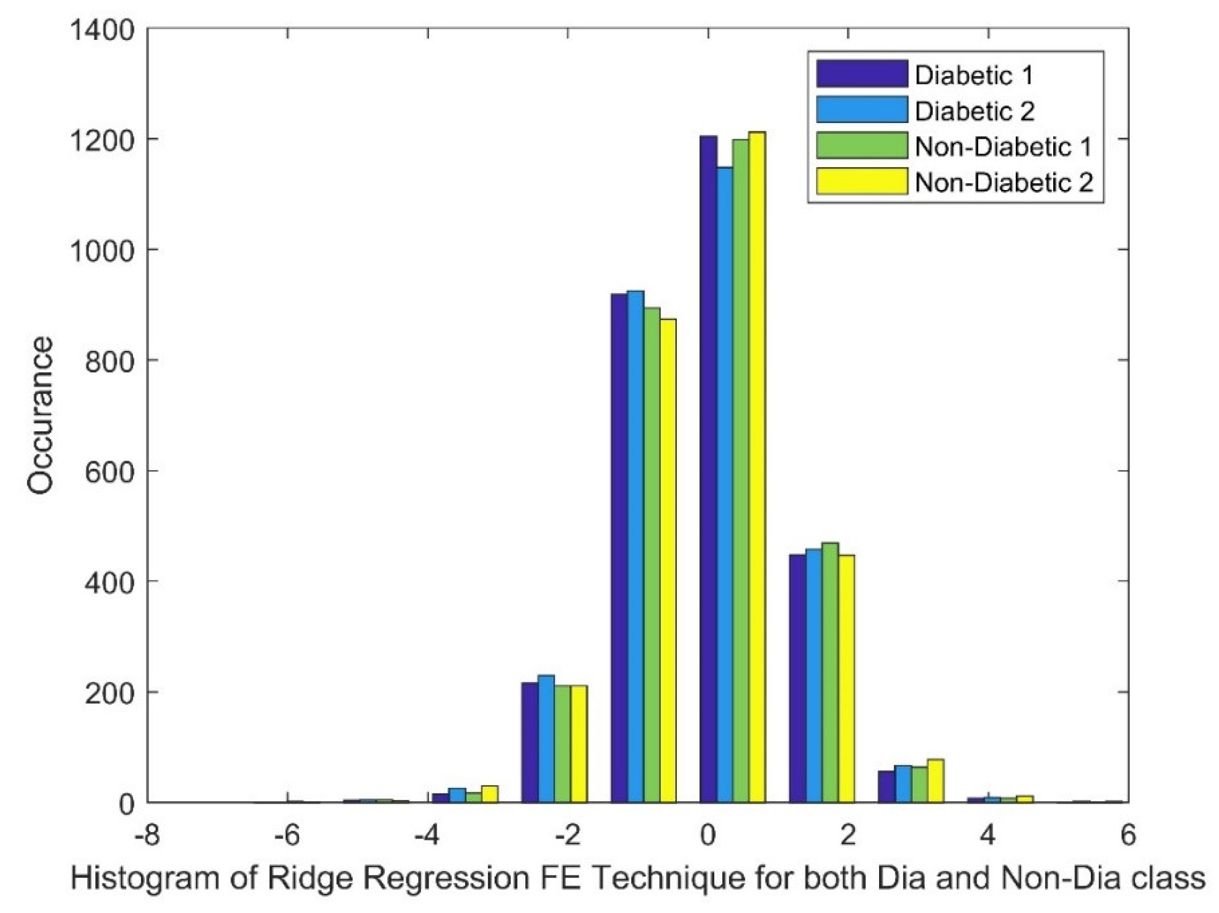
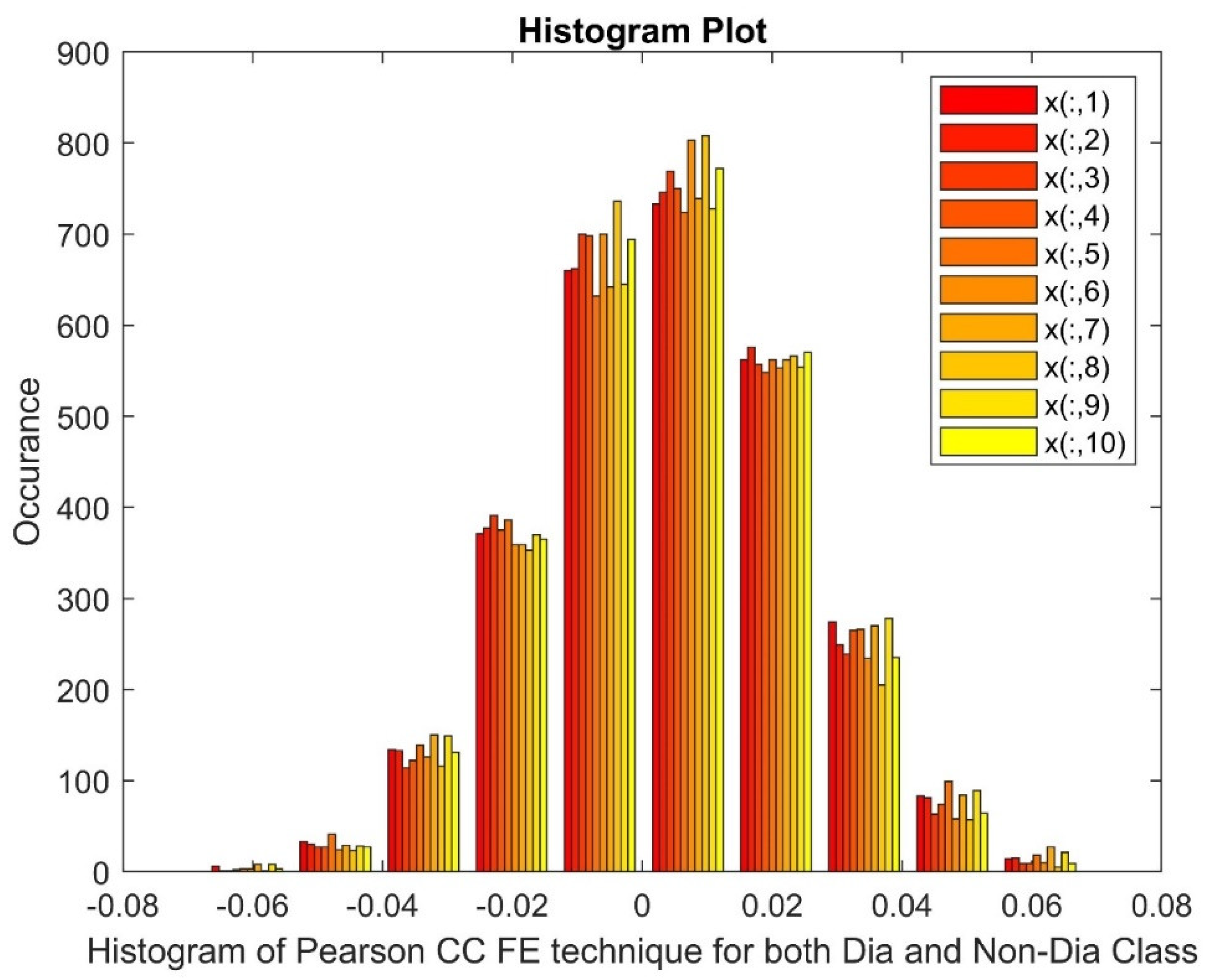
|
Statistical Parameters |
STFT | Ridge Regression | Pearson CC | |||
| Dia P | Non-Dia P | Dia P | Non-Dia P | Dia P | Non-Dia P | |
| Mean | 40.7681 | 40.7863 | 0.0033 | 0.0025 | 0.0047 | 0.0045 |
| Variance | 11745.67 | 11789.27 | 1.3511 | 1.3746 | 0.0004 | 0.0004 |
| Skewness | 19.2455 | 19.2461 | 0.0284 | -0.0032 | 0.0038 | -0.0317 |
| Kurtosis | 388.5211 | 388.5372 | 0.6909 | 0.9046 | -0.1658 | -0.0884 |
| Sample Entropy | 11.0014 | 11.0014 | 11.4868 | 11.4868 | 11.4868 | 11.4868 |
| Shannon Entropy | 0 | 0 | 3.9818 | 3.9684 | 2.8979 | 2.9848 |
| Higuchi Fractal Dimension | 1.1097 | 1.1104 | 2.007 | 2.0093 | 1.9834 | 1.9659 |
| CCA | 0.4031 | 0.0675 | 0.0908 | |||
| S.No. | Parameters | Values | S.No. | Parameters | Values |
|---|---|---|---|---|---|
| 1. | Initial Population (I) | 100 | 6. | Beta (β) | 0.4 |
| 2. | Maximum time of simulation | 10 (s) | 7. | Gamma (γ) | 0.7 |
| 3. | Number of males (M) | 15 | 8. | Roar | 0.25 |
| 4. | Number of hinds (H) | I M | 9. | Fight | 0.4 |
| 5. | Alpha (α) | 0.85 | 10. | Mating | 0.77 |
| Feature selection | DR Techniques | STFT | Ridge Regression | Pearson CC | |||
| Class | Dia P | Non-Dia P | Dia P | Non-Dia P | Dia P | Non-Dia P | |
| BESO | P value <0.05 |
0.4673 | 0.3545 | 0.2962 | 0.2599 | 0.3373 | 0.3178 |
| RDO | P value <0.05 |
0.4996 | 0.4999 | 0.4999 | 0.4883 | 0.4999 | 0.4999 |
| Clinical Situation |
Predicted Values | ||
| Dia | Non-Dia | ||
| Real Values |
Class of Dia | TP | FN |
| Class of non-Dia | FP | TN | |
| Classifiers | STFT | Ridge Regression | Pearson CC | |||
| Train MSE | Test MSE | Train MSE | Test MSE | Train MSE | Test MSE | |
| NLR | 1.59× 10⁻⁵ | 4.84× 10⁻⁶ | 7.29× 10⁻⁶ | 3.25× 10⁻⁵ | 4.36× 10⁻⁵ | 4.1× 10⁻⁴ |
| LR | 1.18× 10⁻⁵ | 3.61× 10⁻⁶ | 1.16× 10⁻⁵ | 1.94× 10⁻⁵ | 9.61× 10⁻⁶ | 3.84× 10⁻⁴ |
| GMM | 1.05× 10⁻⁵ | 2.89× 10⁻⁶ | 1.02× 10⁻⁵ | 1.48× 10⁻⁵ | 2.02× 10⁻⁵ | 8.41× 10⁻⁴ |
| EM | 6.74× 10⁻⁶ | 2.89× 10⁻⁶ | 5.29× 10⁻⁶ | 1.37× 10⁻⁵ | 9.61× 10⁻⁶ | 3.72× 10⁻⁵ |
| LoR | 2.46× 10⁻⁵ | 9× 10⁻⁶ | 2.7× 10⁻⁵ | 3.02× 10⁻⁵ | 4× 10⁻⁶ | 2.92× 10⁻⁵ |
| SDC | 1.28× 10⁻⁵ | 4× 10⁻⁶ | 1.68× 10⁻⁵ | 1.22× 10⁻⁵ | 2.56× 10⁻⁶ | 1.85× 10⁻⁵ |
| SVM (RBF) | 1.88× 10⁻⁶ | 1× 10⁻⁶ | 2.56× 10⁻⁶ | 4.41× 10⁻⁶ | 3.6× 10⁻⁷ | 4.41× 10⁻⁶ |
| Classifiers | STFT | Ridge Regression | Pearson CC | |||
| Train MSE | Test MSE | Train MSE | Test MSE | Train MSE | Test MSE | |
| NLR | 1.43× 10⁻⁵ | 5.29× 10⁻⁵ | 1.44× 10⁻⁵ | 2.21× 10⁻⁵ | 9.41× 10⁻⁵ | 7.06× 10⁻⁵ |
| LR | 3.76× 10⁻⁵ | 2.3× 10⁻⁵ | 7.74× 10⁻⁵ | 1.85× 10⁻⁵ | 2.5× 10⁻⁵ | 2.02× 10⁻⁵ |
| GMM | 4.51× 10⁻⁵ | 1.3× 10⁻⁵ | 6.56× 10⁻⁵ | 3.97× 10⁻⁴ | 6.08× 10⁻⁵ | 3.02× 10⁻⁵ |
| EM | 3.4× 10⁻⁵ | 1.37× 10⁻⁵ | 5.18× 10⁻⁵ | 3.14× 10⁻⁴ | 1.6× 10⁻⁷ | 1.3× 10⁻⁵ |
| LoR | 9.97× 10⁻⁶ | 4× 10⁻⁶ | 9× 10⁻⁶ | 1.76× 10⁻⁵ | 4.9× 10⁻⁷ | 1.68× 10⁻⁵ |
| SDC | 2.21× 10⁻⁵ | 1.6× 10⁻⁵ | 2.81× 10⁻⁶ | 2.81× 10⁻⁴ | 8.1× 10⁻⁷ | 8.65× 10⁻⁵ |
| SVM (RBF) | 2.18× 10⁻⁶ | 1.44× 10⁻⁶ | 5.29× 10⁻⁶ | 4.9× 10⁻⁵ | 4.9× 10⁻⁷ | 8.1× 10⁻⁷ |
| Classifiers | STFT | Ridge Regression | Pearson CC | |||
| Train MSE | Test MSE | Train MSE | Test MSE | Train MSE | Test MSE | |
| NLR | 2.62× 10⁻⁵ | 2.56× 10⁻⁶ | 6.08× 10⁻⁵ | 9× 10⁻⁶ | 5.04× 10⁻⁵ | 6.56× 10⁻⁵ |
| LR | 4.85× 10⁻⁵ | 1.96× 10⁻⁶ | 6.24× 10⁻⁵ | 6.4× 10⁻⁵ | 2.25× 10⁻⁶ | 1.09× 10⁻⁵ |
| GMM | 9.01× 10⁻⁶ | 4.41× 10⁻⁶ | 2.12× 10⁻⁵ | 2.25× 10⁻⁶ | 6.25× 10⁻⁶ | 1.22× 10⁻⁵ |
| EM | 3.51× 10⁻⁵ | 7.29× 10⁻⁶ | 5.48× 10⁻⁵ | 2.81× 10⁻⁵ | 1.69× 10⁻⁶ | 7.84× 10⁻⁶ |
| LoR | 1.39× 10⁻⁵ | 2.25× 10⁻⁶ | 3.02× 10⁻⁵ | 4.84× 10⁻⁶ | 3.6× 10⁻⁷ | 4× 10⁻⁶ |
| SDC | 1.35× 10⁻⁵ | 2.89× 10⁻⁶ | 2.6× 10⁻⁵ | 1.96× 10⁻⁶ | 1.44× 10⁻⁷ | 1.68× 10⁻⁵ |
| SVM (RBF) | 4.25× 10⁻⁷ | 3.6× 10⁻⁷ | 8.1× 10⁻⁷ | 9× 10⁻⁸ | 4× 10⁻⁸ | 2.5× 10⁻⁷ |
| Classifiers | Description |
|---|---|
| NLR | The uniform weight is set to 0.4, while the bias is adjusted iteratively to minimize the sum of least square errors, with the criterion being the Mean Squared Error (MSE). |
| Linear Regression | The weight is uniformly set at 0.451, while the bias is adjusted to 0.003 iteratively to meet the Mean Squared Error (MSE) criterion. |
| GMM | The input sample’s mean covariance and tuning parameter are refined through EM steps, with MSE as the criterion. |
| EM | The likelihood probability is 0.13, the cluster probability is 0.45, and the convergence rate is 0.631, with the condition being MSE. |
| Logistic regression | The criterion is MSE, with the condition being that the threshold Hθ(x) should be less than 0.48. |
| SDC | The parameter Γ is set to 0.5, alongside mean target values of 0.1 and 0.85 for each class. |
| SVM (RBF) | The settings include C as 1, the coefficient of the kernel function (gamma) as 100, class weights at 0.86, and the convergence criterion as MSE. |
| Metrics | Formula |
|---|---|
| Accuracy | |
| F1 Score | |
| Matthews Correlation Coefficient (MCC) | |
| Jaccard Metric | |
| Error Rate | ER = 1 - Accu |
| Kappa |
|
| Feature Extraction | Classifiers | Parameters | |||||
|---|---|---|---|---|---|---|---|
| Accu (%) |
F1S (%) |
MCC | Jaccard Metric (%) |
Error rate (%) | Kappa | ||
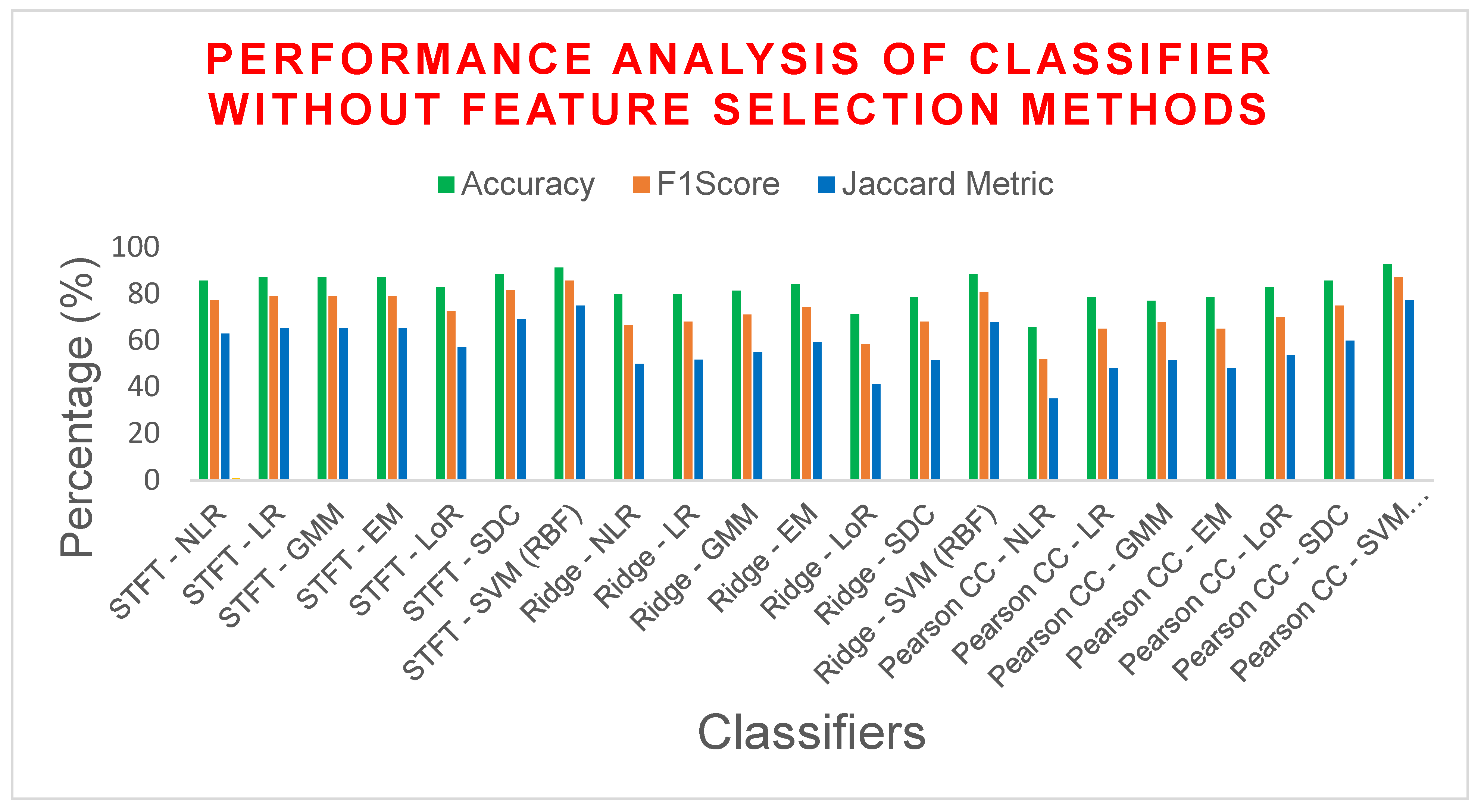
| STFT | NLR | 85.7142 | 77.2727 | 0.6757 | 62.9629 | 14.2857 | 0.6698 |
| LR | 87.1428 | 79.0697 | 0.7021 | 65.3846 | 12.8571 | 0.6985 | |
| GMM | 87.1428 | 79.0697 | 0.7021 | 65.3846 | 12.8571 | 0.6985 | |
| EM | 87.1428 | 79.0697 | 0.7021 | 65.3846 | 12.8571 | 0.6985 | |
| LoR | 82.8571 | 72.7272 | 0.6091 | 57.1428 | 17.1428 | 0.6037 | |
| SDC | 88.5714 | 81.8181 | 0.7423 | 69.2307 | 11.4285 | 0.7358 | |
| SVM (RBF) | 91.4285 | 85.7142 | 0.7979 | 75 | 8.57142 | 0.7961 | |
| Ridge Regression | NLR | 80 | 66.6667 | 0.5255 | 50 | 20 | 0.5242 |
| LR | 80 | 68.1818 | 0.5425 | 51.7241 | 20 | 0.5377 | |
| GMM | 81.4285 | 71.1111 | 0.5845 | 55.1724 | 18.5714 | 0.5767 | |
| EM | 84.2857 | 74.4186 | 0.6348 | 59.2592 | 15.7142 | 0.6315 | |
| LoR | 71.4286 | 58.3333 | 0.3873 | 41.1764 | 28.5714 | 0.375 | |
| SDC | 78.5714 | 68.0851 | 0.5383 | 51.6129 | 21.4285 | 0.5248 | |
| SVM (RBF) | 88.5714 | 80.9524 | 0.7298 | 68 | 11.4285 | 0.7281 | |
| Pearson CC | NLR | 65.7143 | 52 | 0.2829 | 35.1351 | 34.2857 | 0.2695 |
| LR | 78.5714 | 65.1162 | 0.5001 | 48.2758 | 21.4285 | 0.4976 | |
| GMM | 77.1429 | 68 | 0.5385 | 51.5151 | 22.8571 | 0.5130 | |
| EM | 78.5714 | 65.1162 | 0.5001 | 48.2758 | 21.4285 | 0.4976 | |
| LoR | 82.8571 | 70 | 0.58 | 53.8461 | 17.1428 | 0.58 | |
| SDC | 85.7142 | 75 | 0.65 | 60 | 14.2857 | 0.65 | |
| SVM (RBF) | 92.8571 | 87.1795 | 0.8228 | 77.2727 | 7.14285 | 0.8223 | |
| Feature Extraction | Classifiers | Parameters | |||||
|---|---|---|---|---|---|---|---|
| Accu (%) |
F1S (%) |
MCC | Jaccard Metric (%) |
Error rate (%) | Kappa | ||
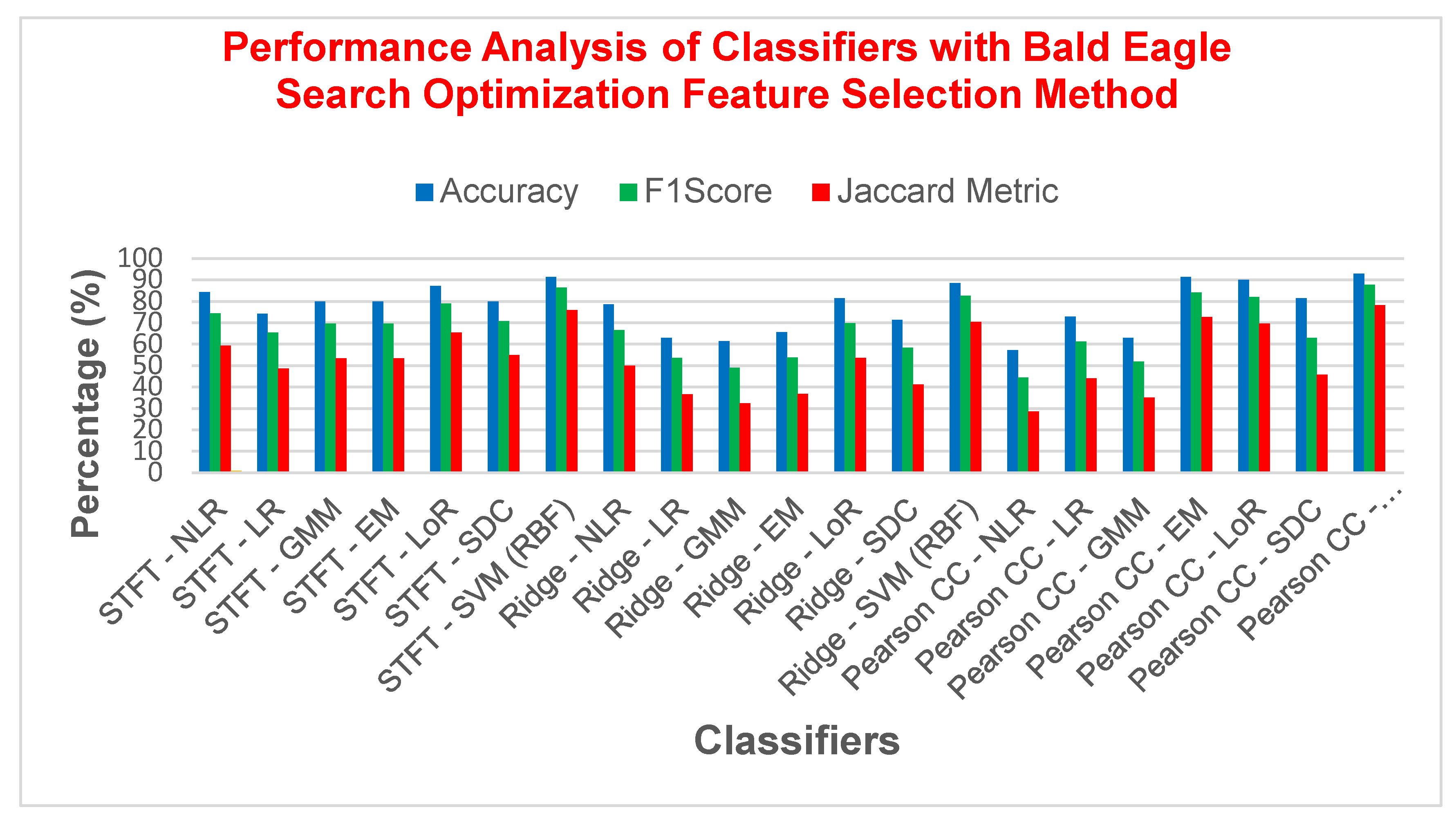
| STFT | NLR | 84.2857 | 74.4186 | 0.6347 | 59.2592 | 15.7142 | 0.6315 |
| LR | 74.2857 | 65.3846 | 0.4987 | 48.5714 | 25.7142 | 0.4661 | |
| GMM | 80 | 69.5652 | 0.5609 | 53.3333 | 20 | 0.5504 | |
| EM | 80 | 69.5652 | 0.5609 | 53.3333 | 20 | 0.5504 | |
| LoR | 87.1428 | 79.0697 | 0.7021 | 65.3846 | 12.8571 | 0.6985 | |
| SDC | 80 | 70.8333 | 0.5809 | 54.8387 | 20 | 0.5625 | |
| SVM (RBF) | 91.4285 | 86.3636 | 0.8089 | 76 | 8.57142 | 0.8018 | |
| Ridge Regression | NLR | 78.5714 | 66.6667 | 0.5185 | 50 | 21.4285 | 0.5116 |
| LR | 62.8571 | 53.5714 | 0.2982 | 36.5853 | 37.1428 | 0.2661 | |
| GMM | 61.4285 | 49.0566 | 0.2262 | 32.5 | 38.5714 | 0.2092 | |
| EM | 65.7142 | 53.8461 | 0.3083 | 36.8421 | 34.2857 | 0.2881 | |
| LoR | 81.4285 | 69.7674 | 0.5674 | 53.5714 | 18.5714 | 0.5645 | |
| SDC | 71.4285 | 58.3333 | 0.3872 | 41.1764 | 28.5714 | 0.375 | |
| SVM (RBF) | 88.5714 | 82.6087 | 0.7573 | 70.3703 | 11.4285 | 0.7431 | |
| Pearson CC | NLR | 57.1428 | 44.4444 | 0.1446 | 28.5714 | 42.8571 | 0.1322 |
| LR | 72.8571 | 61.2244 | 0.4310 | 44.1176 | 27.1428 | 0.4140 | |
| GMM | 62.8571 | 51.8518 | 0.2711 | 35 | 37.1428 | 0.2479 | |
| EM | 91.4285 | 84.2105 | 0.7855 | 72.7272 | 8.57142 | 0.7835 | |
| LoR | 90 | 82.0512 | 0.7517 | 69.5652 | 10 | 0.7512 | |
| SDC | 81.4285 | 62.8571 | 0.5174 | 45.8333 | 18.5714 | 0.5081 | |
| SVM (RBF) | 92.8571 | 87.8048 | 0.8280 | 78.2608 | 7.14285 | 0.8275 | |
| Feature Extraction | Classifiers | Parameters | |||||
|---|---|---|---|---|---|---|---|
| Accu (%) |
F1S (%) |
MCC | Jaccard Metric (%) |
Error rate (%) | Kappa | ||
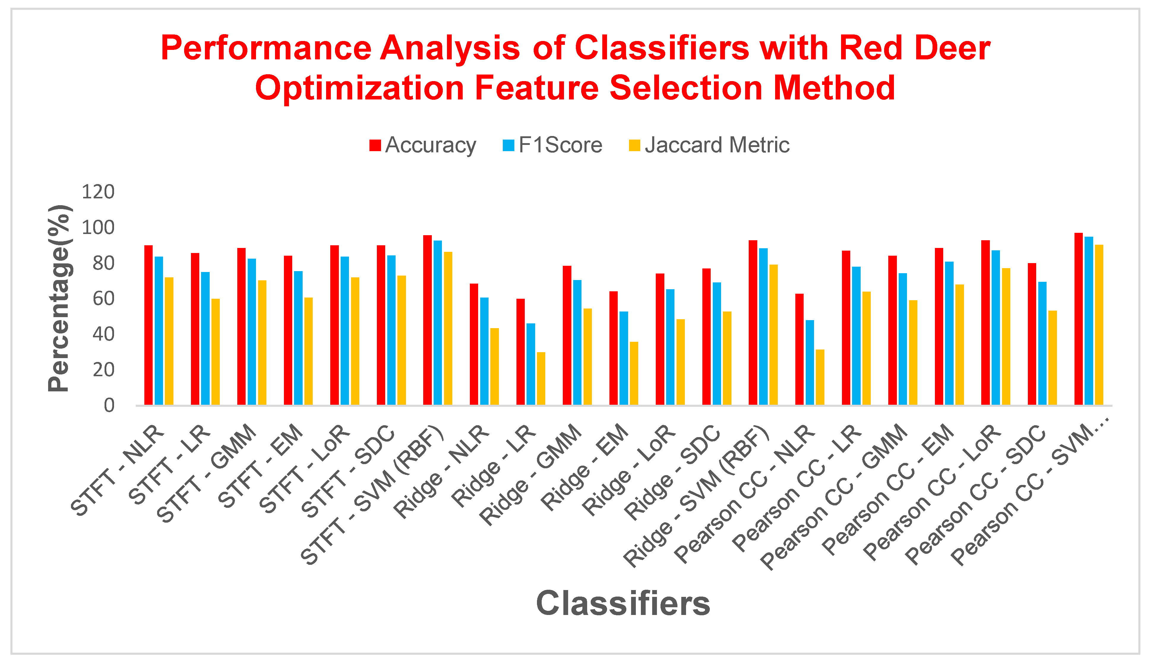
| STFT | NLR | 90 | 83.7209 | 0.7694 | 72 | 10 | 0.76555 |
| LR | 85.7142 | 75 | 0.65 | 60 | 14.2857 | 0.65 | |
| GMM | 88.5714 | 82.6087 | 0.7573 | 70.3703 | 11.4285 | 0.7431 | |
| EM | 84.2857 | 75.5555 | 0.6505 | 60.7142 | 15.7142 | 0.6418 | |
| LoR | 90 | 83.7209 | 0.7694 | 72 | 10 | 0.7655 | |
| SDC | 90 | 84.4444 | 0.7825 | 73.0769 | 10 | 0.7721 | |
| SVM (RBF) | 95.7142 | 92.6829 | 0.8971 | 86.3636 | 4.2857 | 0.8965 | |
| Ridge Regression | NLR | 68.5714 | 60.7142 | 0.4248 | 43.5897 | 31.4285 | 0.3790 |
| LR | 60 | 46.1538 | 0.1813 | 30 | 40 | 0.1694 | |
| GMM | 78.5714 | 70.5882 | 0.5820 | 54.5454 | 21.4285 | 0.5493 | |
| EM | 64.2857 | 52.8301 | 0.2895 | 35.8974 | 35.7142 | 0.2677 | |
| LoR | 74.2857 | 65.3846 | 0.4987 | 48.5714 | 25.7142 | 0.4661 | |
| SDC | 77.1428 | 69.2307 | 0.5622 | 52.9411 | 22.8571 | 0.5254 | |
| SVM (RBF) | 92.8571 | 88.3720 | 0.8367 | 79.1667 | 7.14285 | 0.8325 | |
| Pearson CC | NLR | 62.8571 | 48 | 0.2190 | 31.5789 | 37.1428 | 0.2086 |
| LR | 87.1428 | 78.0487 | 0.6901 | 64 | 12.8571 | 0.6896 | |
| GMM | 84.2857 | 74.4186 | 0.6347 | 59.2592 | 15.7142 | 0.6315 | |
| EM | 88.5714 | 80.9523 | 0.7298 | 68 | 11.4285 | 0.7281 | |
| LoR | 92.8571 | 87.1794 | 0.8228 | 77.2727 | 7.14285 | 0.8223 | |
| SDC | 80 | 69.5652 | 0.5609 | 53.3333 | 20 | 0.5504 | |
| SVM (RBF) | 97.1428 | 95 | 0.93 | 90.4761 | 2.85714 | 0.93 | |
| Classifiers | DR Method | ||
|---|---|---|---|
| STFT | Ridge Regression |
Pearson CC | |
| NLR | O(n2 logn) | O(2n2 log2n) | O(2n2 log2n) |
| LR | O(n2 logn) | O(2n2log2n) | O(2n2 log2n) |
| GMM | O(n2 log2n) | O(2n3 log2n) | O(2n3 log2n) |
| EM | O(n3 logn) | O(2n3 log2n) | O(2n3 log2n) |
| LoR | O(2n2 logn) | O(2n2 log2n) | O(2n2 log2n) |
| SDC | O(n3 logn) | O(2n2 log2n) | O(2n2 log2n) |
| SVM (RBF) | O(2n4 log2n) | O(2n2 log4n) | O(2n2 log4n) |
| Classifiers | DR Method | ||
|---|---|---|---|
| STFT | Ridge Regression |
Pearson CC | |
| NLR | O(n4 logn) | O(2n4 log2n) | O(2n4 log2n) |
| LR | O(n4 logn) | O(2n4 log2n) | O(2n4 log2n) |
| GMM | O(n4 log2n) | O(2n5 log2n) | O(2n5 log2n) |
| EM | O(n5 logn) | O(2n5 log2n) | O(2n5 log2n) |
| LoR | O(2n4 logn) | O(2n4 log2n) | O(2n4 log2n) |
| SDC | O(n5 logn) | O(2n4 log2n) | O(2n4 log2n) |
| SVM (RBF) | O(2n6 log2n) | O(2n4 log4n) | O(2n4 log4n) |
| Classifiers | DR Method | ||
|---|---|---|---|
| STFT | Ridge Regression |
Pearson CC | |
| NLR | O(n5 logn) | O(2n5 log2n) | O(2n5 log2n) |
| LR | O(n5 logn) | O(2n5 log2n) | O(2n5 log2n) |
| GMM | O(n5 log2n) | O(2n6 log2n) | O(2n6 log2n) |
| EM | O(n6 logn) | O(2n6 log2n) | O(2n6 log2n) |
| LoR | O(2n5 logn) | O(2n5 log2n) | O(2n5 log2n) |
| SDC | O(n6 logn) | O(2n5 log2n) | O(2n5 log2n) |
| SVM (RBF) | O(2n7 log2n) | O(2n5 log4n) | O(2n5 log4n) |
| S.No | Author (with Year) | Description of the Population |
Data Sampling |
Machine Learning Parameter |
Accuracy (%) |
|---|---|---|---|---|---|
| 1. | This article | Nordic Islet Transplantation program | Tenfold cross-validation | STFT, RR, PCC, NLR, LR, LoR, GMM, EM, SDC, SVM(RBF) | 97.14 |
| 2. | Maniruzzaman et al. (2017) [46] | PIDD (Pima Indian diabetic dataset) | Cross-validation K2, K4, K5, K10, and JK |
LDA, QDA, NB, GPC, SVM, ANN, AB, LoR, DT, RF |
ACC: 92 |
| 3. | Hertroijs et al. (2018) [47] | Total: 105814 Age(mean): greater than 18 |
Training set of 90% and test set of 10% fivefold cross-validation |
Latent Growth Mixture Modeling (LGMM) | ACC: 92.3 |
| 4. | Deo et al. (2019) [48] | Total: 140 diabetes: 14 imbalanced age: 12–90 | Training set of 70% and 30% test set with fivefold cross-validation, holdout validation |
BT, SVM (L) | ACC: 91 |
| 5. | Akula et al. (2019) [49] | PIDD Practice Fusion Dataset total: 10,000 age: 18–80 |
Training set: 800; test set: 10,000 |
KNN, SVM, DT, RF, GB, NN, NB | ACC: 86 |
| 6. | Xie et al. (2019) [50] | Total: 138,146 diabetes: 20,467 age: 30–80 |
Training set is around 67%, test set is around 33% | SVM, DT, LoR, RF, NN, NB | ACC: 81, 74, 81, 79, 82, 78 |
| 7. | Bernardini et al. (2020) [51] | Total: 252 diabetes: 252 age: 54–72 | Tenfold cross-validation | Multiple instance learning boosting |
ACC: 83 |
| 8. | Zhang et al. (2021) [52] | Total: 37,730, diabetes: 9.4% age: 50–70 imbalanced |
Training set is around 80% test set is around 20% Tenfold cross-validation |
Bagging boosting, GBT, RF, GBM | ACC: 82 |
Disclaimer/Publisher’s Note: The statements, opinions and data contained in all publications are solely those of the individual author(s) and contributor(s) and not of MDPI and/or the editor(s). MDPI and/or the editor(s) disclaim responsibility for any injury to people or property resulting from any ideas, methods, instructions or products referred to in the content. |
© 2024 by the authors. Licensee MDPI, Basel, Switzerland. This article is an open access article distributed under the terms and conditions of the Creative Commons Attribution (CC BY) license (http://creativecommons.org/licenses/by/4.0/).


