The Roots of Gravity in Electrodynamics the Electrodynamics of Electrically Neutral Bodies

Giacomo De Toma

doi:10.20944/preprints202406.1183.v1

Preprint

Hypothesis

The Roots of Gravity in Electrodynamics the Electrodynamics of Electrically Neutral Bodies

This version is not peer-reviewed.

Giacomo De Toma^*

This version is not peer-reviewed.

Downloads

Views

Comments

Submitted:

17 June 2024

Posted:

18 June 2024

You are already at the latest version

Abstract

Coulomb’s law and Newton’s law of gravitation are formally identical. Is it a mere coincidence? It seems to us that physics has answered yes so far, at least tacitly. We, on the other hand, do not believe in chance. Since the alternative to the fact that the strong similarity is only the result of chance is to believe that it is not, and in this case there must be a reason for this similarity, we have chosen the path of investigating the possibility that the two fields are not distinct, but have a common root that we will try to find. We propose an electrodynamics of electrically neutral bodies based on the hypothesis that the Coulomb constant in the case of attraction between charges of opposite sign is slightly greater than that of the case of repulsion between charges of the same magnitude as the previous ones, but of the same sign. If this difference were to exist, even small to the point of not being directly measurable in the laboratory, it could still produce macroscopic effects detectable in the case of large aggregates of charges, even if globally electrically neutral, as happens in the astronomical field. We deduce the electromagnetism of such a model and show the results obtained applying the theory to some significant cases such the light deflection in a gravitational field, a planet perihelion precession, the power radiated by merging black holes, the behaviour of antimatter in a gravitational field and, when available, we compare the predictions with the experimental data.

Keywords:

Gravity

;

week equivalence principle

;

electrodynamics

Subject:

Physical Sciences - Theoretical Physics

This preprints belongs to the Topic

Covariance, Objectivity and Evolution Equations in Either Classical or Quantum Gravity and Quantum Mechanics

1. Introduction

Our model is based on the hypothesis that the strength of the repulsive force between charges of the same magnitude and sign can be slightly less than that of the attractive force that would act between charges of the same magnitude but opposite sign. This difference is very small and impossible to measure in the laboratory, because it is several tens of orders of magnitude lower than the sensitivity of the measurement systems. It can emerge and become measurable for globally neutral systems only when the total value of charges that make up the system has orders of magnitude large enough to make it measurable. And that is gravity.

We will show that the introduction of this hypothesis in electrostatics produces an effect indistinguishable from the gravitational force if the ratio between the total charge contained in the atom and its mass assumes a single value common to all atoms or at most varies within a very narrow range. By total charge we mean the sum of the magnitudes of all positive and negative charges of all the partons in the nucleons and in the pions contained into the nucleus, plus that of the electrons surrounding the nucleus.

Maintaining the focus on electrically neutral bodies, we will develop all the consequences also in the field of magnetism and wave phenomena, arriving at Maxwell’s equations for electrically neutral systems. Or said differently, Maxwell’s equations for gravity.

For this reason, the model we propose develops in a Minkowsky metric space.

In the entire document, when not explicitly expressed, the S.I. units have been adopted.

2. Electrostatic and Gravitational Fields

Note on writing: in this work the electric charges with the superscript sign are to be considered in absolute value. Therefore, the sign to be used in the operations will be spelled out in front of them. Differently from this, when a different use is not evident from the text, a charge indicated without a sign in the superscript will contain the sign inside, thus being able to assume both positive and negative values.

Suppose we place two equal electric charges

q^{+}

and

q^{-}

, but with opposite signs, at a certain distance. It is known that charges attract each other and that the force of attraction has the same magnitude of that exerted by two charges equal to those said, but of the same sign.

The above is expressed in Coulomb’s law which gives in vacuum for point charges the magnitude of the forces:

k_{0} \frac{q^{+} q^{-}}{r^{2}} = k_{0} \frac{q^{+} q^{+}}{r^{2}} = k_{0} \frac{q^{-} q^{-}}{r^{2}} .

(1)

However, reflecting on the fact that the statement expressed by the above equalities has empirical origins, it was born in the laboratory, we can identify in those equalities a simplification that does not take into account their origin and which, if it were to prove incorrect, could have tangible and important consequences. Indeed, when making measurements, it is generally impossible to establish the equality in mathematical terms of the physical quantities being measured, even when the measures coincide. This happens because a measurement is subject to unavoidable limitations that derive from the sensitivity of the instrumentation used, from the statistical nature of the measurement itself and from many other things. It cannot be said that they the measured forces are identically the same in mathematical terms.

Supposing we want to write Coulomb’s law based on experimental evidence, we could more properly write the following equivalences with respect to (1):

f k_{0} \frac{q^{+} q^{-}}{r^{2}} ≃ k_{0} \frac{q^{+} q^{+}}{r^{2}} = k_{0} \frac{q^{-} q^{-}}{r^{2}}

(2)

in which f

\neq 1

, although approximate to it, takes into account a possible difference between attraction and repulsion and

k_{0}

represents the Coulomb’s constant in the case of repulsion. We could also make the matter explicit by naming distinct Coulomb constants to be used in the two cases of attraction and repulsion, but we find it easier to use the constant f.

This is a crucial point for the proposed theory, which requires clearly aiming at the key concept.

The CODATA 2018 value for the Coulomb’s constant is

k_{0} = 8.9875517923 (14) \times 10^{9}

. The number of certain significant figures is eleven. Well, we ask ourselves what electrodynamics would be like if, in the case of the attraction between charges of opposite sign, the Coulomb constant was worth for example

k_{0} \cdot (1 + 9 \times 10^{- 39})

. It is clear that this value would be indistinguishable from the Coulomb constant from the measurement point of view. But, as we will see from the developments we deduce, it would have significant macroscopic consequences.

Now let’s try to deduce the consequences of assuming such a hypothesis and, in particular, what electrodynamics arises from it.

Suppose we have two pairs of charges

Q^{+}

Q^{-}

and

q^{+}

q -

, each pair being in general non-neutral, and that the distance between the charges of each pair is much smaller than that which separates the two pairs (this will be implicit in the reasoning that we will make in the sequel). Indeed, we can also assume that the two charges of each pair are in the same point.

For reasons which will become clear later, we will make use of the following quantities referred to a generic pair of charges

q^{+}

and

q^{-}

the usual net charge: $q_{n} = q^{+} - q^{-}$
the total charge: $q_{T} = q^{+} + q^{-}$
the average charge: $\bar{q} = (q^{+} + q^{-}) / 2$

In the case of a neutral pair it is

q^{+} = q^{-} = q = \bar{q}

and q will be called hemicharge hereinafter.

When, on the other hand, we are dealing with two pairs of charges, the quantity defined here mixed charge will also be used:

Q_{M} = \sqrt{\frac{Q^{+} q^{-} + Q^{-} q^{+}}{2}}

that is null only when both the pairs are replaced by charges of the same sign.

Now let’s try to deduce the consequences of assuming such a hypothesis and, in particular, what electrodynamics arises from it.

Let us now consider the forces acting on each charge exchanged with the charges of the other pair. Each charge will be affected by an attractive and a repulsive force. In particular, the charge

Q^{+}

exchanges the following two forces with the charges of the other pair:

repulsive: $k_{0} \frac{Q^{+} q^{+}}{r^{2}}$ ;
attractive: $f k_{0} \frac{Q^{+} q^{-}}{r^{2}}$ .

The resultant of the two forces will be, assuming it positive if attractive:

f k_{0} \frac{Q^{+} q^{-}}{r^{2}} - k_{0} \frac{Q^{+} q^{+}}{r^{2}}

Similarly, the charge

Q^{-}

exchanges the following two forces with the charges of the other pair:

repulsive: $k_{0} \frac{Q^{-} q^{-}}{r^{2}}$
attractive: $f k_{0} \frac{Q^{-} q^{+}}{r^{2}}$

The resultant of the two forces, assuming the same convention, will be:

f k_{0} \frac{Q^{-} q^{+}}{r^{2}} - k_{0} \frac{Q^{-} q^{-}}{r^{2}}

Therefore, on the pair formed by the charges

Q^{+}

and

Q^{-}

acts a total resulting force F equal to:

F = f k_{0} \frac{Q^{+} q^{-}}{r^{2}} - k_{0} \frac{Q^{+} q^{+}}{r^{2}} + f k_{0} \frac{Q^{-} q^{+}}{r^{2}} - k_{0} \frac{Q^{-} q^{-}}{r^{2}}

or:

F = \frac{k_{0}}{r^{2}} [f (Q^{+} q^{-} + Q^{-} q^{+}) - (Q^{+} q^{+} + Q^{-} q^{-})] .

that, using the defined

Q_{M}

Q_{n}

and

q_{n}

, becomes

F = \frac{k_{0}}{r^{2}} [2 f^{'} Q_{M}^{2} - Q_{n} q_{n}]

(3)

where it is

f^{'} = f - 1

We can write the above equation in vectorial form giving the force acting on the pair made by

q^{+}

and

q^{-}

making evident the two contribution as:

\vec{F} = - 2 f^{'} k_{0} \frac{Q_{M}^{2}}{r^{2}} \vec{u} + k_{0} \frac{Q_{n} q_{n}}{r^{2}} \vec{u}

(4)

being

\vec{u}

the versor pointing the said pair.

If we divide both sides of the above equation by

q_{n}

we get the electric field in the point occupied by

q_{n}

which we could attribute to the pair

Q^{+}

and

Q^{-}

\vec{E} = - 2 f^{'} k_{0} \frac{Q_{M}^{2} / q_{n}}{r^{2}} \vec{u} + k_{0} \frac{Q_{n}}{r^{2}} \vec{u}

(5)

in which we recognize the Coulomb electric field and another term which expresses the effect of the asymmetry between attraction and repulsion introduced by

f^{'}

. As is evident, while the Coulomb field depends only on

Q_{n}

the other term also depends on

q_{n}

and is therefore not identifiable as a physical entity in one-to-one correspondence with only one of the charge systems. This become possible in the case

Q_{n} = 0

2.1. Discussion on Adopting Different Coulomb’s Constants

In discussions with some physicists on the exposed hypothesis - Coulomb’s constant depending on the attractive or repulsive interaction - it was objected that in this way we artificially introduce another force into electrodynamics. In our opinion this objection is trivially unfounded because even in electrodynamics there are two forces. In fact, forces are vectors and, as such, are characterized by three quantities: magnitude, direction and sense. Attraction and repulsion differ by sense. So, they are different forces. In our model we simply add to the difference even a very small one in magnitude, which is worth about

9 \cdot 10^{- 39} k_{0}

We believe that the main driver of this objection is the loss of symmetry which, in many cases, physicists like because it is considered beautiful and, in our opinion, also simplifies reality, thus making the task of describing it easier. We consider these arguments to be devoid of physical sense. Nature has no obligation to satisfy our aesthetic tastes nor our need for simplification.

2.2. Particular Cases

Let us now examine some limiting cases for Eq. (4):

For $Q_{M} = 0$ :

$\vec{F} = k_{0} \frac{Q_{n} q_{n}}{r^{2}} \vec{u}$

which coincides with Coulomb’s law
Only one pair is neutral, suppose $Q_{n} = 0$ :

$\vec{F} = - 2 f^{'} k_{0} \frac{Q \bar{q}}{r^{2}} \vec{u}$

In the particular case in which is, for example, $q^{-} = 0$ we have:

$\vec{F} = - 2 f^{'} k_{0} \frac{Q q / 2}{r^{2}} \vec{u}$
Both pairs are neutrals, i.e. $Q_{n} = 0$ and $q_{n} = 0$ :

$\vec{F} = - 2 f^{'} k_{0} \frac{Q q}{r^{2}} \vec{u}$

being $Q = Q^{+} = Q^{-}$ and $q = q^{+} = q^{-}$ .

For sake of synthesis we can also introduce a further constant:

k_{0}^{'} = 2 k_{0} f^{'}

(6)

2.3. The Gravitational Field

We have seen that with both pairs neutrals the force acting on q is:

{\vec{F}}_{n} = - k_{0}^{'} \frac{Q q}{r^{2}} \vec{u}

(7)

The subscript n of

F_{n}

reminds us that the force is between electrically neutral bodies.

It can be seen that, with the hypotheses made, systems of electrically neutral charges can exchange forces with a non-zero magnitude if it is

f^{'} \neq 0

An attempt to give a physical interpretation to the force in Eq. (7) and possibly estimate

f^{'}

and

k_{0}^{'}

can be done with the help of the following question: do we know a force with the following characteristics?

1): acts between electrically neutral bodies
2): follows the low of the inverse square of the distance
3): it always acts in the same way, that is, it is always and only attractive or always and only repulsive.

Right now, looking for a force with such characteristics among the four fundamental interactions known to physics, we know of only one answer to this very specific question: we only know the force of gravity.

This is the point where the major assumption of this job is done: we assume that the residual force acting between electrically neutral bodies in the case

f^{'} \neq 0

as expressed by the Eq. (7) is what we know as the gravitational force.

Naturally we know that gravity has another important and peculiar property: bodies of different masses placed in the same gravitational field accelerate in the same way. Well, for this to happen it is necessary and sufficient that the ratio between hemicharge and inertial mass of bodies has a value that is common to all the bodies. We will deal with this essential aspect in Section 3.

Differently from what was done in the previous edition, the weak equivalence principle is assumed here as a postulate. This choice is justified by the fact that the main theme discussed here is the nature of gravity, regardless of whether it determines the same acceleration of different bodies immersed in the same field or not.

Well, assuming WEP is true implies that the ratio between hemicharge and mass is a constant in nature, common to all bodies.

Given two neutral bodies of inertial masses M and m, hemicharges respectively Q and q, and assuming the force in Eq. (7) representing the gravitational force, we have:

k_{0}^{'} \frac{Q q}{r^{2}} = G \frac{M m}{r^{2}}

(8)

identifying the gravitational masses with the inertial ones.

Denoted by

χ

the ratio between the emicharge and the inertial mass of each body we have:

χ = \frac{Q}{M}

χ = \frac{q}{m}

or said differently:

Q = χ M

q = χ m

Then we can write Eq. (8), dropping

1 / r^{2}

, as follows::

k_{0}^{'} Q q = k_{0}^{'} χ^{2} M m = G M m

obtaining:

G = k_{0}^{'} χ^{2}

(9)

We can also write the field that the hemicharge Q generates in the point where is q in vector form as:

{\vec{E}}_{n} = \frac{{\vec{F}}_{n}}{q} = - k_{0}^{'} \frac{Q}{r^{2}} \vec{u_{r}}

(10)

being the

\vec{u_{r}}

the versor pointing q from Q. Again the subscript n of the field

{\vec{E}}_{n}

reminds us that it is the electric field generated by an electrically neutral body.

Another consequence that immediately follows Eq. (10) is that, being this residual field of electrostatic nature, it will manifest all the already known properties of these fields, including the fact of propagating at a finite speed equal to that of the light and to originate electromagnetic waves.

As already said,

f^{'}

must be very small, at least within the limits of the sensitivity of measurements of the electrostatic forces that can actually be carried out. But, it is possible to imagine that, however small it may be, it could express tangible effects in the case of large aggregates of electrically neutral pairs (for the sake of brevity in the following they will be called

n e u t r a l

n e u t r a l s

), the number of which is such as to make its effect noticeable, as we find in the astronomical scales.

It is of great interest to be able to correlate the electric field just found with the gravitational field

\vec{g}

as understood in mechanics, which provides the acceleration of a body in it.

We can note that, for a body of mass m and hemicharge

q = m χ

, it is:

q {\vec{E}}_{n} = m \vec{g}

but it is also:

q {\vec{E}}_{n} = m χ {\vec{E}}_{n} = m \vec{g}

from which we have:

\vec{g} = χ {\vec{E}}_{n}

that shows us that

χ

is the conversion factor that transforms the electric field into the gravitational one.

We can anticipate that, as will be evident in the results obtained in the section dedicated to the magnetism associated to neutral bodies, this conversion factor is applicable to all electromagnetic fields.

The Gauss’s law tell us that the flux of

{\vec{E}}_{n}

through a closed surface S is equal to the total hemicharge contained in it divided by

ϵ_{0}^{'}

which leads to:

\nabla \cdot {\vec{E}}_{n} = - \frac{ρ}{ϵ_{0}^{'}}

(11)

where

ρ

is the hemicharge density and ∇ the operator:

\nabla = (\frac{\partial}{\partial x}, \frac{\partial}{\partial y}, \frac{\partial}{\partial z})

We can also show the Eq. (11) in terms of

\vec{g}

just multiplying it by the conversion factor

χ

and remembering that

ρ = ρ_{m} χ

, obtaining:

\nabla \cdot \vec{g} = - 4 π G ρ_{m}

(12)

where

ρ_{m}

is the mass density.

Likewise in the above equation and as will be evident in the chapter dedicated to magnetism and wave phenomena, it will be possible to write the complete Maxwell equations basing them entirely on masses, mass current densities and the universal gravitational constant G, albeit with an important reservation.

2.4. Gravitational Potential

Adopting the usual conventions of the potential, for the hemicharge Q we have:

Φ_{n} = - k_{0}^{'} \frac{Q}{r}

(13)

that is related to the field of Eq( 10) through the following equation:

{\vec{E}}_{n} = - \nabla Φ_{n}

(14)

with the already know mechanical correspondents:

Φ_{g} = - G \frac{M}{r}

(15)

\vec{g} = - \nabla Φ_{g}

(16)

It seems useless to recall how one can pass from one to the other through the conversion factor

χ

2.5. Few Considerations on the Adopted Method

It could be objected that the approach based on the identification of different values of

k_{0}

in relation to the sign of the product of the charges is ill-posed, since the choice of

k_{0}

is arbitrary. For example, in the c.g.s. it is equal to 1. In reality, even if we moved in the c.g.s. we would find the same thing. That is, after having defined the unit of both positive and negative charge, the Stat-coulomb, the problem would arise of verifying that, taking two unitary charges but of opposite sign, located at a unitary distance, the force exchanged between them has the same magnitude as the one exchanged between unit charges with the same sign. Also in that setting we could assume that, considering unit positive and negative charges distant 1 cm, in the repulsive case the strength of the force is 1 Dyne, while in the case of attraction is

f \neq 1

Dyne.

Another topic we want to draw attention to is the method used to derive the quantities. As we have already seen in the electrostatic case, the hypothesized residual electric field generated by globally neutral charge systems, which would be manifested by gravity, was obtained with only one hypothesis, the one according to which

f^{'} \neq 0

can be assumed, then applying the usual and known laws of electrostatics to the pairs of interacting charges, obtaining the final result using the principle of superposition of affects. Well, this will be the way to proceed also in the following paragraphs, therefore also when we go to look for what happens in the case of moving neutral bodies.

There too we will apply the laws of electrodynamics of moving charges, also using special relativity and the transformation laws of scalar and vector fields under Lorentz transformations, to the single charges or pair of interacting charges, obtaining the generated electromagnetic fields, and in the end we will add up the effects.

Therefore, all that will derive from it, if it exists, will be none other than the electrodynamics of neutral systems in which the fundamental role is played by the value of

f^{'}

. Electrodynamics assumes

f^{'} = 0

, therefore it does not associate any electromagnetic field with neutral bodies. If instead we get something, that is electromagnetic fields and all the already known phenomenology, it will only be traced back to the supposedly non-zero value of

f^{'}

. Under this hypothesis, gravity would only be the electrodynamics of electrically neutral bodies.

A recurring objection to the proposed theory is that the introduction of an asymmetry between attraction and repulsion actually introduces a new force. We consider the objection baseless because already in classical electrodynamics the attractive and repulsive forces are different forces. In fact, when passing from one to the other, a transformation must be performed which determines a rotation equal to

π

. Our theory adds only a very small change in the magnitude of the force to the transformation, on the order of

10^{- 38}

of it.

The last consideration is relevant to the Eq. (5). More than one physicist has shown doubts about what the equation implies, highlighting the fact that in this way the one-to-one correspondence between the electric field and the charge that generates it is lost, as there is a term on the right side of the equation, the first, which depends on both pairs. In this regard, it is worth noting that, as shown in the previous paragraphs, this term represents the ratio between the gravitational force and the hemicharge. This, obviously, does not represent an electric field analogous to that of electrostatics. It is good to keep in mind that forces originated by different interactions can be added, while different fields cannot. The cited equation should be seen as an equation that would be obtained by immersing a charged body q simultaneously in an electric and a gravitational field. Such a body would be subject to both gravitational and electrostatic forces, and these forces would be summable. But if you then divide the resultant by the value of the charge you obtain two terms that compare poorly. The ratio between the electrostatic force and the charge would give the electric field, while the ratio between the gravitational force and the charge would give a vector that cannot be traced back to any field normally used in physics.

3. The Charge-to-Mass Ratio and Electric Constants Calculation

Our aims are mainly focused on:

1) try to calculate even roughly the value of the hemicharge-to-mass ratio

2) calculate

k_{0}^{'}

3.1. Particles

Before entering into the model, a summary is useful about the structure of the nucleons, i.e. the proton and the neutron.

According to the Standard Model of particles the constituents of the nucleons are quarks, antiquarks and gluons.

Defined x the fraction of the momentum of the nucleon carried by the quark in a fast moving (infinite momentum) reference frame,

u (x)

and

\bar{u} (x)

the distribution of the up quark and the antiquark,

d (x)

and

\bar{d} (x)

the distribution of the down quark and the antiquark,

s (x)

and

\bar{s} (x)

the distribution of the strange or heavier quarks and the antiquark and indicating with the subscript p and n the nucleon the distribution are referred to, they are:

For the proton:

\int_{0}^{1} [u_{p} (x) - {\bar{u}}_{p} (x)] d x = 2

\int_{0}^{1} [d_{p} (x) - {\bar{d}}_{p} (x)] d x = 1

\int_{0}^{1} [s_{p} (x) - {\bar{s}}_{p} (x)] d x = 0

For the neutron:

\int_{0}^{1} [u_{n} (x) - {\bar{u}}_{n} (x)] d x = 1

\int_{0}^{1} [d_{n} (x) - {\bar{d}}_{n} (x)] d x = 2

\int_{0}^{1} [s_{n} (x) - {\bar{s}}_{n} (x)] d x = 0

To be remember that the antiquarks belong only to the see quarks and, then, the sea quarks is globally electrically neutral. Therefore, the study of the sea quark distribution can be done using the distribution of antiquarks, especially for the up and down quarks, who are present also as valence quarks.

The dependence of the introduced densities on x is complex and has been the subject of considerable theoretical and experimental developments on which we cannot dwell here. What interests us at the end is the total charge contained in the neutron and proton. Since this is easy for valence quarks, we now focus on the sea quark. The main data we will use come from the publication of D. F. Geesaman and P. E. Reimer (The Sea of Quarks and Antiquarks in the Nucleon: a Review [5]).

A first assumption relevant to strange and heavier quarks is that their contribution is the same in the neutron and in the proton, i.e.,

s_{n} (x) = s_{p} (x)

and

{\bar{s}}_{n} (x) = {\bar{s}}_{p} (x)

Until 1989 a good fit with the experimental data was with

\bar{d} (x) = \bar{u} (x)

. Subsequently, when the New Muon Collaboration (NMC) at CERN first reported [6] a deep inelastic scattering measurement of the Gottfried sum [7] of the difference in the structure functions F2 for the proton and the neutron. An asymmetry was highlighted by D. F. Geesaman and P. E. Reimer in [5] which lead to assume valid the following equation:

\int_{0}^{1} [\bar{d} (x) - \bar{u} (x)] d x = 0.13

Moreover, Yang, Liang et al. (see [8]) have proposed a proton mass decomposition from QCD energy momentum tensor, broken down into four contributions as follow:

quark energy (kinetic): 32%
gluonic field strength energy: 36%
quark scalar condensate 9%
trace anomalous gluonic contribution 23%. Consists of contributions from condensates of all quark flavors, including the strange, charm, bottom, and top quarks.

The simplified assumptions on which we will base our model for hemicharge estimate are:

the electric charges considered are only those of the quarks, both valence and see quarks of which we obviously also consider the antiparticles
the total rest mass of u and d quarks is $9 %$ of its mass
the sea quarks of both neutron and proton has been subject to a fine tuning by means of the comparison between the measured value of G and the calculated ones. The minimum error has been achieved through the adoption of the following equations:

$\int_{0}^{1} [\bar{d_{p}} (x) - \bar{u_{p}} (x)] d x = 0.64$

$\int_{0}^{1} [\bar{d_{n}} (x) - \bar{u_{n}} (x)] d x = 0.73$
we consider the anomalous gluonic contribution made of only strange quarks and anti-quarks.

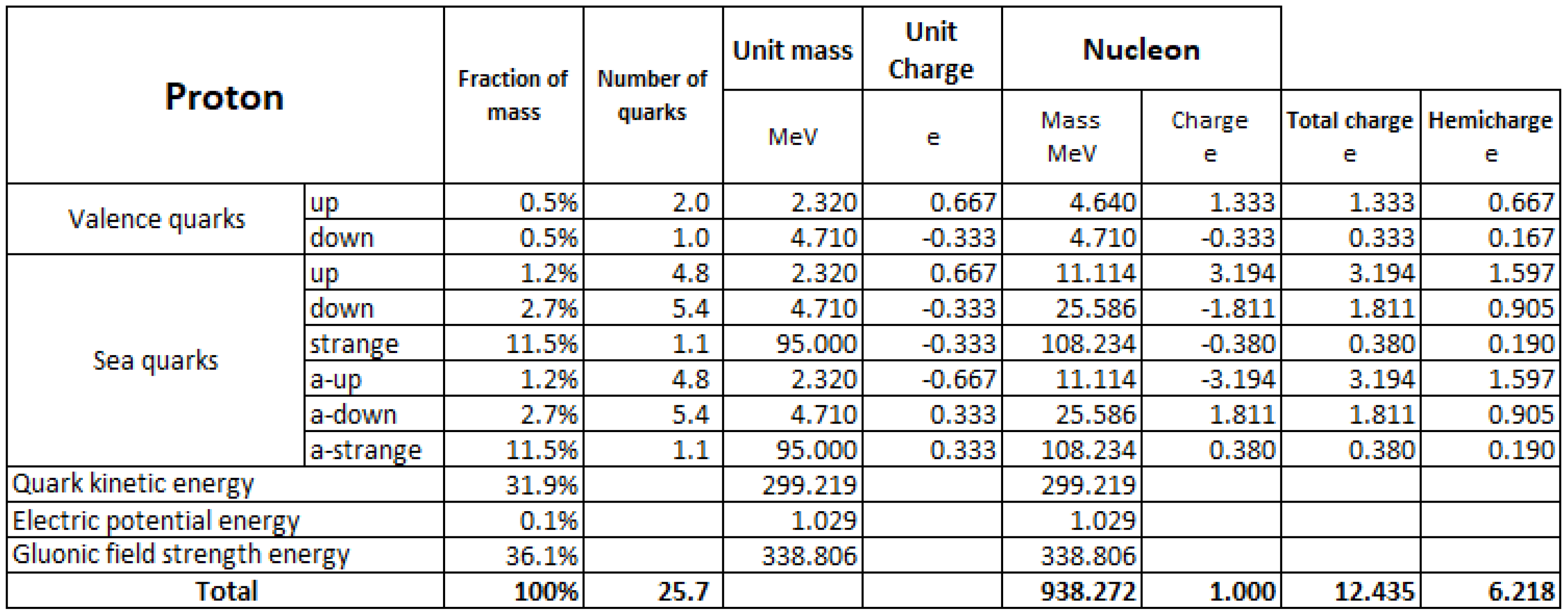
With the adopted assumption we calculate first the hemicharge of the neutron and proton as in the tables in Appendix F from which we have the hemicharge of the unbound neutron

q_{N 0} = 6.709 e

and the average charge of the unbound proton

q_{P 0} = 6.218 e

These numbers allow us to calculate the hemicharge-to-mass ratio of:

the unbound neutron:

χ_{N 0} = \frac{q_{N 0}}{m_{N 0}} = 6.4174 \cdot 10^{8}

the hydrogen atom (protium):

χ_{H} = \frac{q_{H}}{m_{H}} = 6.4312 \cdot 10^{8}

the unbound proton:

χ_{P 0} = \frac{q_{P 0}}{m_{P 0}} = 5.9557 \cdot 10^{8}

the electron:

χ_{e} = \frac{e}{2 m_{e}} = 8.7941 \cdot 10^{10}

It can be noted that the values of

χ

of the neutron and the hydrogen atom are very close and that the ratio between them and the

χ_{e}

is approximately equal to

α

, the fine structure constant. We are not now able to explain this last observation. Furthermore, considering the approximations made for the calculation of the hemicharges of the neutron and the proton, we can hypothesize that the different values of

χ

obtained could be attributable to errors, also consistent with admitting the WEP to be true that imply a unique

χ

for the neutral matter. Therefore, we assume that in general the value of

χ

of the baryonic matter is unique and defined as follows:

χ = α χ_{e} = 6.4174 \cdot 10^{8}

The simplification assumed above, unique

χ

for baryonic matter, is adopted for simplicity and because the topic is not essential for the proposed theory. However, we would like to point out that, beyond the doubts about the correctness of the estimates of the hemicharges of nucleons and atoms, we still consider the topic of the real values of the hemicharge-to-mass ratio of the various elements of the periodic table open and worthy of further study since, if they were to change from one element to another, it could result in WEP violation of the baryonic matter, at least within the proposed theory. Which, however, as we will see, is certainly expected for leptonic matter, as can be understood from the value of

χ_{e}

, which is the same as that of positronium.

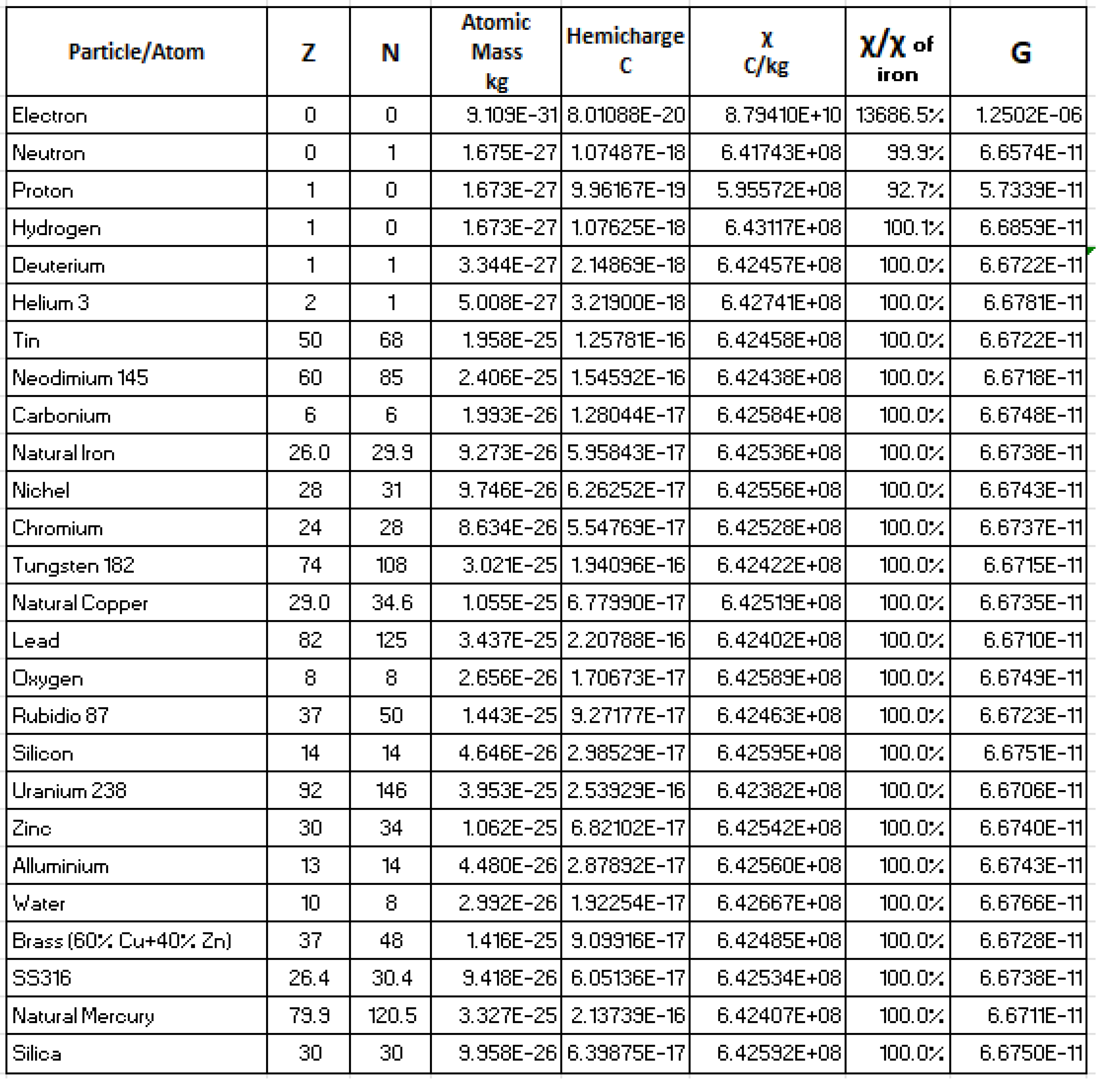
Returning again to the topic of the dependence of the calculation of G on the value of

χ

, Figure 2 shows a table in which the G of some elements has been calculated, based on the composition of their atomic nucleus and the mass defect. As you can see, these values differ from one to another, typically to the third decimal place, except for light elements such as hydrogen. This can be traced back to the fact that the values of

χ

of the neutron and the proton obtained with our estimate differ, producing consequences in relation to the different neutron/proton ratio of each element, both because the mass defect per nucleon is not a constant, but varies from nucleus to nucleus.

This dependence of G on the elements leads one to think that, if true, the universality of G, and therefore of the WEP, is not true even for baryonic matter. Indeed, hundreds of measurements of G made show that the value does not converge towards the expected single one, and may differ from each other by as much as eighteen sigma, making G the known physical constant with the least precision. No more than four significant figures are known with certainty.

The model we proposed could provide an explanation for this experimental evidence. And the suspicion that this may be true is supported by the data in the table in Figure 1, which compares the measured and calculated values of G from some experiments.

Since it is not essential for the development of the proposed theory, and in any case there is a possible incorrect modeling of the nucleus and of the relationship between quarks, with their charge, and its mass, in the remaining part of this work this aspect is left aside and a single value will be used for

χ

, under the simplifying hypothesis that it has a single value for the baryonic matter.

3.2. $k_{0}^{'}$ Calculation

We have seen that it is

G = k_{0}^{'} χ^{2}

from which we obtain

k_{0}^{'}

as follows:

k_{0}^{'} = \frac{G}{χ^{2}} = 1.6207 \cdot 10^{- 28}

using the above value for

χ

and the CODATA2018 value for G.

3.3. The Photon

To describe the motion of a photon in a gravitational field we started consistently with the paradigm that underlies this work, according to the motion is determined by forces acting in a Minkowskian space. In our model only electromagnetic forces act over long ranges, of which gravimagnetic forces are the expression in the case of neutral bodies. Therefore, we interpret the experimental observation of the deflection of light in a gravitational field as due to an electrodynamic action on the light, then on the photons on which we must admit that a force that bends its trajectory acts. And since the long-range forces that we have available in our scheme are only the electromagnetic ones, which act on electric charges, we are forced to admit that the photon carries electric charges, with null net value, then a neutral pairs of charges. Therefore, in order to calculate the trajectory of a photon in a gravitational field we need to know its hemicharge.

We treat the photon as a particle of mass

ε / c^{2}

, being

ε

the photon’s energy, to which we have to associate a hemicharge-to-mass ratio as usual, to obtain the hemicharge. It is worth adding here that, given the equivalence between mass and energy, we could generally have set up the work using the hemicharge to energy ratio instead of the hemicharge to mass ratio. This would have made it less strange to have to talk about the mass of a photon. Here it must be understood as a measure of its energy.

We do not have a theory that allows us to associate a hemicharge with a photon. As a first attempt we have chosen to use the

χ

. However, from the simulation of the deflection of the photon grazing the Sun (see the dedicated appendix) we had obtained a deflection equal to half of that expected, as also occurs when treating the photon according to classical mechanics. But since the experiment must prevail over idea, we decided to multiply

χ

by two to obtain the hemicharge of the photon that provided the expected deflection, i.e. we set:

q_{p} = 2 χ \frac{ε}{c^{2}}

and we adopt for the hemicharge-to-mass ratio of the photon:

χ_{p} = 2 α χ_{e} = α \frac{e}{m_{e}} = 1.2835 \cdot 10^{9}

(17)

As will be seen in the dedicated appendix, the found

χ_{p}

is the one that works properly.

It results that G acting between photons is nearly four times the CODATA2018 G. Instead, the G acting in the gravitational interaction between photons and common matter is two times the CODATA2018 G.

It seems very interesting to evaluate the impact of these deductions in the astronomical field on a galactic scale in which, according to our model, the attraction between photons and matter must be doubled and that between photons and photons quadrupled.

It should be mentioned that the author, following the development of this work, developed a photon model as can be read in [19]. Said model predicts that the speed of the photon depends on its energy and decreases with it. The speed of light c is the limit towards which the speed of the photon tends as its energy approaches zero. However, in the applications that will follow in this document, in particular the deflection of light in the gravitational field of the Sun, we will simulate a ray of light in the visible spectrum which, whose photons have energies in the order of a few eV, practically have a velocity c. Thus, the dependence of speed on energy will be neglected.

3.4. New Electric Constants Calculation for Gravity

As previously said, we calculated

k_{0}^{'}

from G and

χ

obtaining:

k_{0}^{'} = 1.6207 \cdot 10^{- 28}

We have then been in the position to calculate also

f^{'}

, the vacuum permittivity and the vacuum permeability as follow:

f^{'} = \frac{k_{0}^{'}}{2 k_{0}} = 9.0161 \cdot 10^{- 39}

ϵ_{0}^{'} = \frac{1}{4 π k_{0}^{'}} = 9.8204 \cdot 10^{26}

μ_{0}^{'} = \frac{1}{ϵ_{0}^{'} c^{2}} = 1.1330 \cdot 10^{- 44}

The values of

k_{0}^{'}

and

f^{'}

are too small and impossible to be measured in the lab.

4. Magnetism from Gravity

A moving charged particle produce a magnetic field. Transposing the theme on the Neutrals we can ask ourselves the following two questions:

What does produce a moving Neutral of hemicharge Q?
How a moving Neutral of hemicharge Q acts on another of hemicharge q?

In the following sections we’ll try to give an answer to both the questions.

4.1. Moving Bodies

4.1.1. Point Particles

Since a Neutral of mass M can be seen as a pair of charges

Q^{+}

and

Q^{-}

of opposite signs, we could start with considering the formula giving the magnetic field B generated by the moving charge

Q^{+}

at a velocity

\vec{v_{1}}

, i.e.:

{\vec{B}}^{+} = \frac{μ_{0}}{4 π} \frac{Q^{+}}{r^{2}} {\vec{v}}_{1} \times {\vec{u}}_{r} = \frac{k_{0}}{c^{2}} \frac{Q^{+}}{r^{2}} {\vec{v}}_{1} \times {\vec{u}}_{r}

where

{\vec{u}}_{r}

is the unit vector applied in

Q +

and pointing the point P in the space where the

{\vec{B}}^{+}

is calculated and a possible other charge can be placed.

Let now suppose that in P is placed the positive charge

q^{+}

of a body of mass m moving with a velocity

{\vec{v}}_{2}

. Due to its velocity in the magnetic field

{\vec{B}}^{+}

, on the charge

q^{+}

will act the magnetic component of the Lorenz’s force:

{\vec{F}}_{1} = q^{+} {\vec{v}}_{2} \times {\vec{B}}^{+}

therefore

{\vec{F}}_{1} = q^{+} {\vec{v}}_{2} \times (\frac{k_{0}}{c^{2}} \frac{Q^{+}}{r^{2}} {\vec{v}}_{1} \times {\vec{u}}_{r})

and finally:

{\vec{F}}_{1} = \frac{k_{0}}{c^{2}} \frac{Q^{+} q^{+}}{r^{2}} {\vec{v}}_{2} \times ({\vec{v}}_{1} \times {\vec{u}}_{r})

Since the magnetic force depends on the electric one, as we see also in the above equation, in our theory the Coulomb’s constants to be used will be

k_{0}

for pairs of charges of equal sign while, for those of opposite sign

f k_{0}

Lets now consider the negative charge

Q^{-}

of the mass M, equal in value but with negative sign, obviously co-moving with

Q^{+}

. In this case the magnetic force between

Q^{-}

and

q^{+}

will assume the following expression:

\vec{F_{2}} = - \frac{f k_{0}}{c^{2}} \frac{Q^{-} q^{+}}{r^{2}} \vec{v_{2}} \times (\vec{v_{1}} \times {\vec{u}}_{r})

The resultant force acting on

q^{+}

will be:

\vec{R^{+}} = \vec{F_{1}} + \vec{F_{2}} = \frac{k_{0}}{c^{2}} \frac{Q^{+} q^{+}}{r^{2}} \vec{v_{2}} \times (\vec{v_{1}} \times {\vec{u}}_{r}) - \frac{f k_{0}}{c^{2}} \frac{Q^{-} q^{+}}{r^{2}} \vec{v_{2}} \times (\vec{v_{1}} \times {\vec{u}}_{r})

that, remembering that is

Q^{+}

Q^{-}

=Q, is:

\vec{R^{+}} = - \frac{f^{'} k_{0}}{c^{2}} \frac{Q q^{+}}{r^{2}} \vec{v_{2}} \times (\vec{v_{1}} \times {\vec{u}}_{r})

(18)

Now we need to complete the

N e u t r a l s

scenario, and we do it by considering also the

q^{-}

of the mass m in P, that is negative but equal in vale to

q^{+}

and obviously co-moving with her. The resultant magnetic component of the Lorenz’s force acting on her will be:

\vec{F_{1}} + \vec{F_{2}} = - \frac{f k_{0}}{c^{2}} \frac{Q^{+} q^{-}}{r^{2}} \vec{v_{2}} \times (\vec{v_{1}} \times {\vec{u}}_{r}) + \frac{k_{0}}{c^{2}} \frac{Q^{-} q^{-}}{r^{2}} \vec{v_{2}} \times (\vec{v_{1}} \times {\vec{u}}_{r})

which, after the same operations become:

\vec{R^{-}} = - \frac{f^{'} k_{0}}{c^{2}} \frac{Q q^{-}}{r^{2}} \vec{v_{2}} \times (\vec{v_{1}} \times {\vec{u}}_{r})

(19)

that is exactly equivalent to the Eq.( 18) being

q^{+} = q^{-} = q

So, we can say that on the

N e u t r a l

made by

q^{+}

and

q^{-}

(e.g. the mass m) acts a total magnetic force given by:

\vec{R} = \vec{R^{+}} + \vec{R^{-}} = - \frac{2 f^{'} k_{0}}{c^{2}} \frac{Q q}{r^{2}} \vec{v_{2}} \times (\vec{v_{1}} \times {\vec{u}}_{r}) = - \frac{k_{0}^{'}}{c^{2}} \frac{Q q}{r^{2}} \vec{v_{2}} \times (\vec{v_{1}} \times {\vec{u}}_{r})

(20)

And now we can obtain the magnetic field generated by a moving

N e u t r a l

of hemicharge Q and velocity

\vec{v}

, that is:

{\vec{B}}_{n} = - \frac{k_{0}^{'}}{c^{2}} \frac{Q}{r^{2}} \vec{v} \times {\vec{u}}_{r} = \frac{\vec{v}}{c^{2}} \times {\vec{E}}_{n}

(21)

and remembering that it is:

k_{0}^{'} \frac{Q q}{r^{2}} = G \frac{M m}{r^{2}}

we can also re-write Eq.( 20) and Eq.( 21) in more Newtonian form, putting in evidence the masses and the gravitational field

\vec{g}

generated by the mass M:

- \frac{G}{c^{2}} \frac{M m}{r^{2}} {\vec{v}}_{2} \times ({\vec{v}}_{1} \times {\vec{u}}_{r}) = m {\vec{v}}_{2} \times (\frac{{\vec{v}}_{1}}{c^{2}} \times \vec{g})

(22)

We therefore introduce the field gravimagnetic, the

{\vec{B}}_{g}

, generated by a moving neutral body as:

{\vec{B}}_{g} = \frac{\vec{v}}{c^{2}} \times \vec{g}

(23)

and being:

\vec{g} = χ {\vec{E}}_{n}

we see that:

{\vec{B}}_{g} = χ {\vec{B}}_{n}

(24)

which confirms what has been said about the conversion factor

χ

of the electric field into the gravitational field. Also the gravimagnetic field

B_{g}

χ

times the magnetic field

B_{n}

Now, we can state that a moving neutral mass M generates a magnetic field related to the gravity that it generates, the gravimagnetic field. Moreover, we see that, on another moving neutral body of mass m in that generated field, acts a force. We can therefore talk of a gravimagnetism.

Therefore, we can re-write the gravimagnetic force acting on the mass m in Eq.( 22) as:

\vec{F} = m {\vec{v}}_{2} \times {\vec{B}}_{g}

(25)

Finally we are able to write the total force that a gravitational field

\vec{g}

and a gravimagnetic field

{\vec{B}}_{g}

act on a body of mass m moving with velocity

\vec{v}

exactly as we do for the electric charges using the Lorentz’s force, that we here will rename g-Lorentz’s force in order to remember that we are talking about neutral masses and gravimagnetic fields, as follows:

\vec{F} = m (\vec{g} + \vec{v} \times {\vec{B}}_{g})

(26)

Of course we have obtained the above equation starting from the original Lorentz’s force that we could write for an hemicharge q moving in field containing the

{\vec{E}}_{n}

and

{\vec{B}}_{n}

as follows:

\vec{F} = q ({\vec{E}}_{n} + \vec{v} \times {\vec{B}}_{n})

(27)

from which we obtain the mechanical form just multiplying both terms in brackets by the conversion factor

χ

and the hemicharge q by its reciprocal, i.e.

m / q

We are getting things already employed in the initial gravimagnetism setup. However, in our case the magnetic field is not introduced as an artifice necessary to be able to model gravity through Maxwell’s equations. In our case the magnetic field is real and is coupled to the electric field because the whole phenomenon takes place fully within the electrodynamics sphere, although associated with bodies having a zero net charge. Our results only depend, as already repeated several times, on the initial hypothesis, i.e. that it could be

f^{'} \neq 0

As a first use of the results it looks notable considering the simple case of bodies M and m moving with equal speeds, i.e.

\vec{v_{1}} = \vec{v_{2}} = \vec{v}

and

{\vec{u}}_{r}

orthogonal to them pointing m. In this case the force acting on m is:

\vec{F} = - \frac{G}{c^{2}} \frac{M m}{r^{2}} \vec{v} \times (\vec{v} \times {\vec{u}}_{r})

(28)

and since it is:

\vec{v} \times (\vec{v} \times {\vec{u}}_{r}) = - v^{2} {\vec{u}}_{r}

by using this result int the Eq.( 28) we obtain:

\vec{F} = - \frac{v^{2}}{c^{2}} m \vec{g}

(29)

being

\vec{g}

the gravity generated by M, that is clearly repulsive.

This is a very interesting result which, in our opinion, requires in-depth studies aimed at understanding whether and what effects it can produce at an astrophysical or even cosmological level.

4.1.2. Field Generated by a Neutral Mass Current

Suppose we have an indefinite mass distribution uncharged (from here on "wire"), moving at

\vec{v}

with respect to an inertial reference system S. Let it be

Γ

the mass flow through a surface orthogonal to

\vec{v}

as measured in S.

In such a situation in the frame S we have a linear mass distribution

λ_{m}

given by:

λ_{m} = \frac{Γ}{v}

to which corresponds a hemicharge linear distribution:

λ_{Q} = λ_{m} χ

On neutral particle with hemicharge q at rest in S, placed at a distance d form the wire (we’ll neglect the cross dimension of the wire with respect to d), would act a gravitational force given by:

F g = 2 k_{0}^{'} \frac{λ_{Q}}{d} q

Let now suppose that the particle moves with the same velocity

\vec{v}

of the wire, and at the distance d. Let it be

S^{'}

an inertial reference system co-moving with the particle.

We want now to compare the forces between the wire and the particle in both the reference frames.

First of all we need the hemicharge linear density

λ_{Q}^{'}

S^{'}

We know that, due to the Lorentz’s contraction, the relation between the linear densities evaluated in the two frames is:

λ_{Q} = \frac{λ_{Q}^{'}}{\sqrt{1 - \frac{v^{2}}{c^{2}}}}

from which we obtain:

λ_{Q}^{'} = λ_{Q} \sqrt{1 - \frac{v^{2}}{c^{2}}}

Therefor, in

S^{'}

the gravitational attraction of the wire on q will be:

F^{'} g = 2 k_{0}^{'} \frac{λ_{Q}^{'}}{d} q = 2 k_{0}^{'} \frac{λ_{Q} \sqrt{1 - \frac{v^{2}}{c^{2}}}}{d} q = F_{g} \sqrt{1 - \frac{v^{2}}{c^{2}}}

Since the increase in momentum exerted by the forces in the two references must be the same in the direction orthogonal to the

\vec{v}

, we can obtain the force

F_{g}^{"}

that should act in S from

F_{g}^{'}

using the following:

F_{g}^{"} Δ t = F_{g}^{'} Δ t^{'}

F_{g}^{"} = F_{g}^{'} \frac{Δ t^{'}}{Δ t}

where

Δ t

and

Δ t^{'}

are short time intervals in the two frames related by:

Δ t = \frac{Δ t^{'}}{\sqrt{1 - \frac{v^{2}}{c^{2}}}}

and also

\frac{Δ t^{'}}{Δ t} = \sqrt{1 - \frac{v^{2}}{c^{2}}}

obtaining

F_{g}^{"} = F_{g} (1 - \frac{v^{2}}{c^{2}})

(30)

So, in S the attraction is reduced by the amount:

β^{2} F_{g}

as we have already seen in the case of the two co-moving neutral particles, that we explained in terms of magnetic field associated to the gravity of moving particles. We can then conclude that, as it happens in the usual electrodynamics, a neutral current (mass flow) produce a magnetic field. It is notable again that its action is repulsive.

In order to see better the contribution of all the terms we can write

β^{2} F_{g}

with all the parameter contained and we obtain:

β^{2} F_{g} = \frac{μ_{0}^{'}}{2 π} \frac{I_{Q}}{d} q v

where:

I_{Q} = λ_{Q} v = χ Γ

We can therefore conclude that straight mass flow

Γ

with velocity v produce a magnetic field:

B_{n} = \frac{μ_{0}^{'}}{2 π} \frac{I_{Q}}{d}

whose action is repulsive. Therefore, if we define the vector

\vec{I_{Q}} = λ_{Q} \vec{v}

, the vectorial form of the above equation is:

{\vec{B}}_{n} = - \frac{μ_{0}^{'}}{2 π d} \vec{I_{Q}} \times \vec{u}

(31)

where

\vec{u}

is the versor pointing the position in which we are considering

{\vec{B}}_{n}

We can again find the gravimagnetic field

{\vec{B}}_{g}

generated by the mass flow

Γ

after the due substitutions:

{\vec{B}}_{g} = - \frac{2 G}{c^{2} d} \vec{Γ} \times \vec{u}

(32)

and confirm that it is:

{\vec{B}}_{g} = χ {\vec{B}}_{n}

The same can be achieved using the results obtained for moving masses in the previous paragraph.

Using the already found mechanical counterparts of the constants, we can rewrite the last gravimagnetic field as:

{\vec{B}}_{g} = - \frac{μ_{g}}{2 π d} \vec{Γ} \times \vec{u}

(33)

confirming that, as already announced in the first chapter, we do not need to know

k_{0}^{'}

completely specified, being

{\vec{B}}_{g}

dependent only on G, to which

μ_{g}

is related.

Moreover, through the well know tools of the vector analysis, we know that it will be:

\nabla \times {\vec{B}}_{g} = - \frac{\vec{j}}{ϵ_{g} c^{2}}

with

\vec{j}

being the mass current density.

4.2. Accelerated Bodies

Now we’ll analyze what happens if a neutral body accelerates.

4.2.1. Gravitational Waves

From the electrodynamics we know that an accelerated point charge q produces electromagnetic radiation, at some position

\vec{r}

in space and at some time t according to the following:

{\vec{E}}_{r} (\vec{r}, t) = - \frac{1}{4 π ϵ_{0}} \frac{q}{c^{2} r^{'}} \vec{a_{p}} (t - r^{'} / c) = - k_{0} \frac{q}{c^{2} r^{'}} \vec{a_{p}} (t - r^{'} / c) = - r^{'} \frac{E^{'}}{c^{2}} \vec{a_{p}} (t - r^{'} / c)

(34)

in which

\vec{r^{'}}

is the retarded position and

\vec{a_{p}} (t - r^{'} / c)

the component of the acceleration perpendicular to the line of sight between

\vec{r}

and the retarded position of the charge.

We will use Eq.( 34) to build the wave produced by a

N e u t r a l

, but coming back to the electric force acting on a charge in

\vec{r}

due to the radiation.

So, if Q is the accelerating charge that produce the radiation and q the test charge in

\vec{r}

, then the force will be:

{\vec{F}}_{r} (\vec{r}, t) = q {\vec{E}}_{r} (\vec{r}, t) = - k_{0} \frac{Q q}{c^{2} r^{'}} \vec{a_{p}} (t - r^{'} / c) .

(35)

As usual, we will consider two

N e u t r a l s

and calculate the four forces between each charge of a pair and each other charge of the other pair.

In particular, the

n e u t r a l

accelerating will be the one of hemicharge Q, the test

n e u t r a l

will be the q one.

By applying the Eq.( 35) with the usual symbols we obtain for the resultant acting between the two

n e u t r a l s

{\vec{F}}_{R} (\vec{r}, t) = - \frac{k_{0}}{c^{2} r^{'}} {\vec{a}}_{p} (t - r^{'} / c) (Q^{+} q^{+} + Q^{-} q^{-} - f Q^{+} q^{-} - f Q^{-} q^{+})

that after usual operations becomes:

{\vec{F}}_{R} (\vec{r}, t) = 2 f^{'} k_{0} \frac{Q q}{c^{2} r^{'}} {\vec{a}}_{p} (t - r^{'} / c) = k_{0}^{'} \frac{Q q}{c^{2} r^{'}} {\vec{a}}_{p} (t - r^{'} / c) = - r^{'} \frac{E_{n}^{'} q}{c^{2}} {\vec{a}}_{p} (t - r^{'} / c)

From which we obtain the radiated electric field by dividing by q:

{\vec{E}}_{n R} = \frac{{\vec{F}}_{R} (\vec{r}, t)}{q} = - r^{'} \frac{E_{n}^{'}}{c^{2}} {\vec{a}}_{p} (t - r^{'} / c)

(36)

that, being radiated by a neutral body, can be seen as a gravitational wave. In fact, using our conversion factor

χ

we can also write the Eq.( 36) in term of radiated gravitational field as follows:

{\vec{g}}_{R} = - r^{'} \frac{g^{'}}{c^{2}} {\vec{a}}_{p} (t - r^{'} / c)

(37)

If compared with Eq.( 34), Eq.( 36) tells us that an accelerating body radiates as any charge. The formula to be used to calculate the field of the radiation is the usual, except for the sign, but the hemicharge have to be used instead of the charge, and

k_{0}^{'}

must replace

k_{0}

, if not directly operate with

\vec{g}

Of course a magnetic field perpendicular to the electric one will be associated:

c {\vec{B}}_{n R} = \vec{e^{'}} \times {\vec{E}}_{n R}

Again, using the conversion factor

χ

we can write the equivalent in mechanical terms:

c {\vec{B}}_{g R} = \vec{e^{'}} \times {\vec{g}}_{R}

4.2.2. Radiated Power by Accelerating Bodies

With the results obtained in the previous paragraph we are ready to calculate the power radiated by an accelerating

n e u t r a l

in the case of velocity orthogonal to the acceleration.

First of all we remember the relativistic Larmor formula given for a charge q whose acceleration is in magnitude a:

P = \frac{2}{3} k_{0} \frac{q^{2} a^{2}}{c^{3}} γ^{4}

Retracing the process by which Larmor obtained his formula, with the simple substitution of our parameters and electrical quantities such as

k_{0}^{'}

and the hemicharge Q, we obtain the formula for the power radiated by a body of mass M, acceleration a and hemicharge Q as follows:

P_{g} = \frac{2}{3} k_{0}^{'} \frac{Q^{2} a^{2}}{c^{3}} γ^{4}

(38)

The above equation can also be written in more mechanical terms through the due substitutions, giving the following:

P_{g} = \frac{2}{3} G \frac{M^{2} a^{2}}{c^{3}} γ^{4}

(39)

4.3. Magnetic Induction by Gravity

Suppose we have a rectangular coil with sides a and b disposed orthogonally to a uniform gravimagnetic field

{\vec{B}}_{g}

. Furthermore, suppose that one side of the loop, for example the side a of mass M, moves at constant speed

\vec{v}

in the direction in which the area of the coil increases.

We have already seen that, on a neutral body of mass q moving into a gravimagnetic field

{\vec{B}}_{g}

with velocity

\vec{v}

acts a force

\vec{F}

given by:

\vec{F} = M \vec{v} \times {\vec{B}}_{g}

λ_{m}

is the linear mass of the moving side of the coil, then on it will a act force given by:

\vec{F} = a λ_{m} \vec{v} \times {\vec{B}}_{g}

parallel to the axis of a.

We can introduce the flux of the gravimagnetic field through the loop

Φ = a b B_{g}

. Since:

v = \frac{d b}{d t}

then

a v B_{g} = a \frac{d b}{d t} B_{g} = \frac{d Φ}{d t}

that show that we find the flux rule also in the gravimagnetic field, obtaining the equivalent of the emf, that now will be interpreted as difference of the gravitational potential and call gmf.

We can generalize the result remembering the Faraday’s observations on which base also in the condition of loop at rest in a region where the magnetic field is changing with time, electric fields are generated. It is this electric field which drives the electrons around the wire and so is responsible for the

e m f

in a stationary circuit when there is a changing magnetic flux.

We could, applying the adopted method to obtain the gravimagnetic fields studying the behaviour of each charge and summing up the effects.

We can, without more effort, state that also fot the gravimagnetic field is valid the general low:

\nabla \times \vec{g} = - \frac{\partial {\vec{B}}_{g}}{\partial t}

(40)

5. Lorentz Transformations of the Fields

In this chapter we will briefly cover some topics related to the transformations of the fields

{\vec{E}}_{n}

and

{\vec{B}}_{n}

when passing from an inertial reference frame to another inertial reference frame moving with respect to the first at a constant velocity, usually parallel to the x axis. Therefore, we will limit the scope of our interest to the special relativity, keeping also in mind the applications we want to address. We will use the results obtained in electrodynamics of moving charges and, following the method now familiar, we will apply it to any charge composing a neutral, and obtain the result for the neutral just applying the principle of superposition of effects.

5.1. The Four-Vector of $ρ$ and $\vec{j}$

Here we indicate with

ρ

and

\vec{j}

respectively the hemicharge density and the hemicharge current density. We want to show here that the two indicated quantities form a four-vector in the same way as the usual electric charge and electric current density do. This is because this feature makes possible the invariance under Lorentz transformations of Maxwell’s equations. We have then to see that, given

\vec{J} = (ρ c, \vec{j})

and its Lorentz-boosted counterparts

{\vec{J}}^{'} = (ρ^{'} c, {\vec{j}}^{'})

, it is:

ρ^{2} c^{2} - \vec{j} \cdot \vec{j} = ρ^{' 2} c^{2} - {\vec{j}}^{'} \cdot {\vec{j}}^{'}

The conservation of the charge requires that

ρ = γ ρ_{0}

being

ρ_{0}

the proper charge density, that is Lorentz invariant. It means that we can write:

\vec{J} = (ρ c, \vec{j}) = (ρ c, ρ \vec{v}) = (γ ρ_{0} c, γ ρ_{0} \vec{v}) = ρ_{0} γ (c, \vec{v})

and since

γ (c, \vec{v})

is the four-velocity, which is a four-vector, we have that

\vec{J}

is a four-vector.

We can apply the above result separately for both the

ρ^{+}

and

ρ^{-}

of our neutral body. Due to the linearity of the problem and knowing that it is

ρ^{+} = ρ^{-} = ρ

, we conclude that also the hemicharge current density is a four-vector.

5.2. The Lorentz Formula for the Potentials for a Charge Moving with Constant Velocity

Suppose we have the usual neutral pair of hemicharge Q moving along the x-axis with velocity v. And, for simplicity, we suppose that a time time t the pair is in the origin. We have already seen how to write the potential in the electrostatic case in Eq( 13). In the relativistic case it specialize as follows:

ϕ (x, y, z, t) = - k_{0}^{'} γ \frac{Q}{{[γ^{2} {(x - v t)}^{2} + y^{2} + z^{2}]}^{1 / 2}}

(41)

being:

β = \frac{v}{c}

γ = \frac{1}{\sqrt{1 - β^{2}}}

The vector potential

\vec{A}

is given by:

\vec{A} = \frac{\vec{v}}{c^{2}} ϕ (x, y, z, t)

that in terms of the components for this case provides:

A_{x} = - k_{0}^{'} γ \frac{Q v}{{[γ^{2} {(x - v t)}^{2} + y^{2} + z^{2}]}^{1 / 2}}

A_{y} = A_{z} = 0

5.3. The Fields of a Point Charge with a Constant Velocity

From the potentials found in the previous paragraph we can get the electric field

{\vec{E}}_{n}

and the magnetic field

{\vec{B}}_{n}

generated by a moving neutral Q by the usual rules:

{\vec{E}}_{n} = - \nabla ϕ - \frac{\partial \vec{A}}{\partial t}

{\vec{B}}_{n} = \nabla \times \vec{A}

The three components of the electric field

{\vec{E}}_{n}

at the time t at the point

(x, y, z)

are:

E_{n x} = - k_{0}^{'} Q γ \frac{x - v t}{{[γ^{2} {(x - v t)}^{2} + y^{2} + z^{2}]}^{3 / 2}}

E_{n x} = - k_{0}^{'} Q γ \frac{y}{{[γ^{2} {(x - v t)}^{2} + y^{2} + z^{2}]}^{3 / 2}}

E_{n x} = - k_{0}^{'} Q γ \frac{z}{{[γ^{2} {(x - v t)}^{2} + y^{2} + z^{2}]}^{3 / 2}}

The magnetic field

{\vec{B}}_{n}

is:

{\vec{B}}_{n} = \frac{\vec{v}}{c^{2}} \times {\vec{E}}_{n}

the components of which are

B_{n x} = 0

B_{n y} = \frac{- v E_{n z}}{c^{2}}

B_{n z} = \frac{v E_{n y}}{c^{2}}

5.4. Motion of a Planet around a Moving Star

As a first application of the fields found in the previous paragraph we model here the so-called problem of the two bodies in which one having much greater mass than that of the other body. Therefore we will consider the large one, a star, as having uniform rectilinear motion at constant velocity

{\vec{v}}_{s}

on the x axis of an inertial reference system. In the application to a real case we’ll say which one.

Said

Q_{s}

and

\vec{r} = (x_{s}, y_{s}, z_{s})

respectively the hemicharge and the position vector of the star, its motion will be described by the following equations:

$x_{s} (t) = v_{s} t$
$y_{s} (t) = 0$
$z_{s} (t) = 0$

The three components of the electric field

{\vec{E}}_{n}

it generates at the time t at the point

(x, y, z)

are:

E_{n x} = - k_{0}^{'} Q_{s} γ_{s} \frac{x - v_{s} t}{{[γ_{s}^{2} {(x - v_{s} t)}^{2} + y^{2} + z^{2}]}^{3 / 2}}

E_{n y} = - k_{0}^{'} Q_{s} γ_{s} \frac{y}{{[γ_{s}^{2} {(x - v_{s} t)}^{2} + y^{2} + z^{2}]}^{3 / 2}}

E_{n z} = - k_{0}^{'} Q_{s} γ_{s} \frac{z}{{[γ_{s}^{2} {(x - v_{s} t)}^{2} + y^{2} + z^{2}]}^{3 / 2}}

The magnetic field

{\vec{B}}_{n}

is:

{\vec{B}}_{n} = \frac{\vec{v_{s}}}{c^{2}} \times {\vec{E}}_{n}

the components of which are

B_{n x} = 0

B_{n y} = \frac{- v_{s} E_{n z}}{c^{2}}

B_{n z} = \frac{v_{s} E_{n y}}{c^{2}}

The force acting on the planet will be:

\vec{F} = q ({\vec{E}}_{n} + \vec{v} \times {\vec{B}}_{n})

where q is its hemicharge and

\vec{v}

its velocity.

\vec{p}

is the momentum of the body, we know that it is:

\vec{F} = \frac{d \vec{p}}{d t}

and also that:

\frac{d \vec{p}}{d t} = \frac{d}{d t} (m_{0} γ \vec{v}) = m_{0} (\dot{γ} \vec{v} + γ \vec{a})

with

β = \frac{v}{c}

\dot{β} = \frac{\vec{a} \cdot \vec{v}}{v c}

γ = \frac{1}{\sqrt{1 - β^{2}}}

\dot{γ} = γ^{3} β \dot{β}

It is therefore

\frac{d \vec{p}}{d t} = m_{0} γ^{3} β \dot{β} \vec{v} + m_{0} γ \vec{a}

then it must be:

q ({\vec{E}}_{n} + \vec{v} \times {\vec{B}}_{n}) = m_{0} γ^{3} β \dot{β} \vec{v} + m_{0} γ \vec{a}

from which we obtain

\vec{a} = \frac{χ_{p}}{γ} ({\vec{E}}_{n} + \vec{v} \times {\vec{B}}_{n}) - γ^{2} β \frac{\vec{a} \cdot \vec{v}}{v c} \vec{v}

(42)

We will use this equation to calculate the orbits of Mercury and the Earth around the Sun in a dedicated paragraph.

6. Maxwell Equations for Gravity

By putting together the obtained results at this point, we are able to write the Maxwell equations for the fields

{\vec{E}}_{n}

and

{\vec{B}}_{n}

associate to electrically neutral bodies. They are:

\nabla \cdot \vec{E_{n}} = - 4 π k_{0}^{'} ρ

(43)

\nabla \times {\vec{E}}_{n} = - \frac{\partial {\vec{B}}_{n}}{\partial t}

(44)

\nabla \cdot {\vec{B}}_{n} = 0

(45)

c^{2} \nabla \times {\vec{B}}_{n} = - 4 π k_{0}^{'} \vec{J} + \frac{\partial {\vec{E}}_{n}}{\partial t}

(46)

In the above equations

ρ

is the hemicharge density and

\vec{J}

is the hemicharge current density which, as we demonstrated in the paragraph Section 5.1, form a four-vector. Therefore it is useful to highlight the fact that the equations we have arrived at are invariant under Lorentz transformations. This, in addition to the radical difference in foundation, makes them very different from those developed in the frame of GEM.

7. Application of the Theory to Some Cases

We here show the application of the exposed theory to some significant cases, mostly known to nearly all people. The cases of the light deflection in a gravitational field and the perihelion precession of Mercury have been integrated numerically, using the software Octave 7.3.0. Details on the implementation of the models are in appendixes.

7.1. Radiated Power of Merging Black Holes

Considering the Larmor formula we have derived for a neutral mass (Eq. 39) and applying it to the synchrotron radiation, it is possible to attempt an estimation of the radiated power of two massive bodies rotating around the common mass center (e.i. two merging black holes).

In such a case, supposing the two bodies having masses

M_{1}

and

M_{2}

as point-like, orbiting around the common mass center with accelerations

a_{1}

and

a_{2}

, the total power radiated should be:

P_{g} = \frac{2 G}{3 c^{3}} (M_{1}^{2} a_{1}^{2} γ_{1}^{4} + M_{2}^{2} a_{2}^{2} γ_{2}^{4})

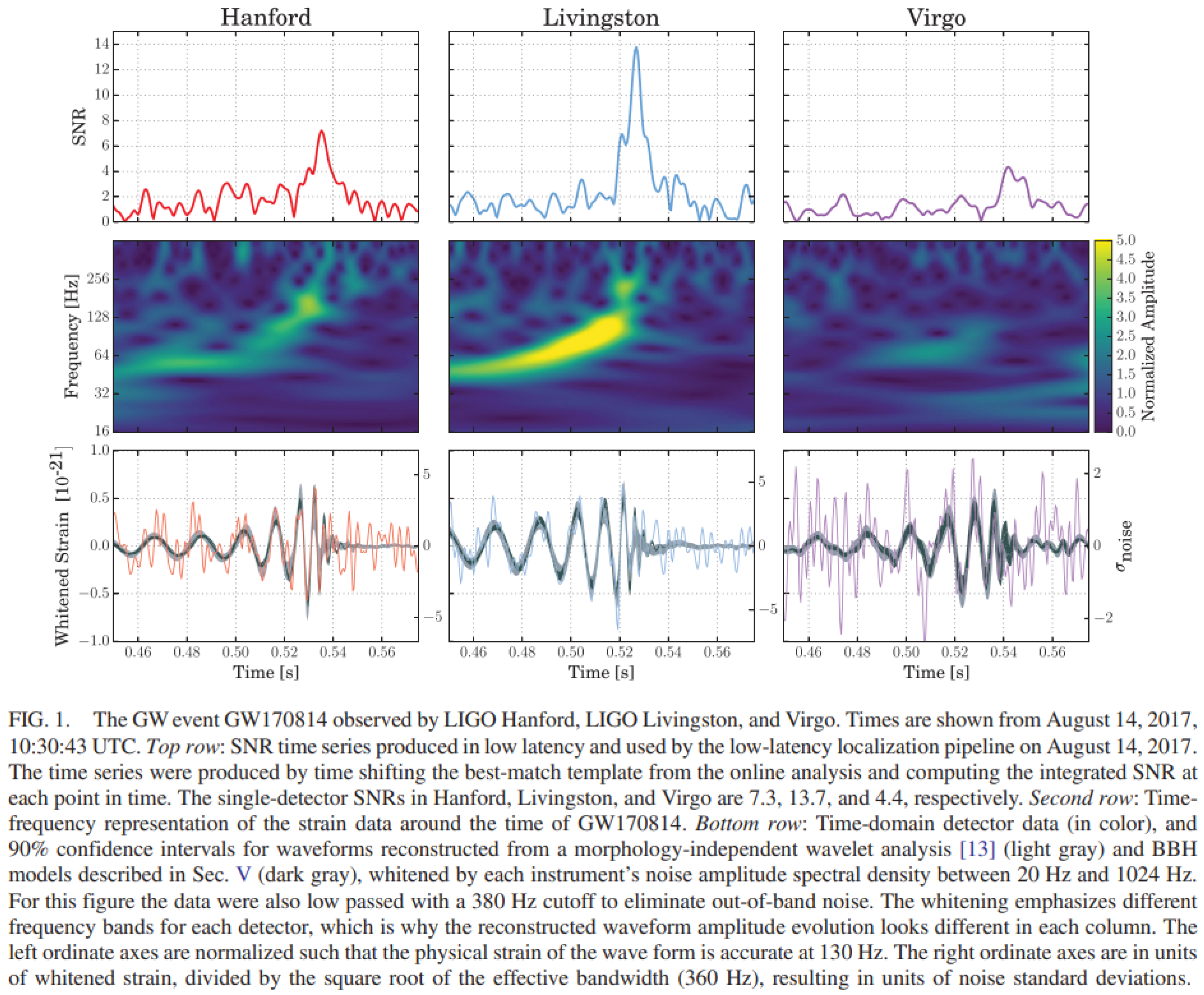
The simulated case in rough way is the instant of the peak luminosity of the event of black hole coalescence whose gravitational waves were detected on August 12, 2017 at 10:30:43 UTC by the Advanced Virgo detector and the two Advanced LIGO detectors described by B.P. Abbott et al. in their paper ”A Three-Detector Observation of Gravitational Waves from a Binary Black Hole Coalescence” [1].

The main data such as the black holes masses are taken from the cited paper as well as the frequency in the moment of the peak luminosity that has been got in approximate way from the picture in Appendix G.

Applying the above equation to the case of two bodies, one of mass

M_{1} = 30.5

solar mass the other

M_{2} = 25.3

solar mass, rotating at 257 km of mutual distance around the common mass center at a frequency of

105 H z

, the parameter to be used for the above equation are:

$M_{1} = 6.067 \times 10^{31}$ kg
$M_{2} = 5.032 \times 10^{31}$ kg
frequency of revolution: $f = 105$ Hz
angular speed of revolution: $ω = 2 π f = 659.7$ $\frac{r a d}{s}$
orbital radius of $M_{1}$ : $r_{1} = 116, 466$ m
orbital radius of $M_{2}$ : $r_{2} = 140, 403$ m
$β_{1} = 0.256$
$β_{2} = 0.309$
$γ_{1} = 1.0346$
$γ_{2} = 1.0514$
$a_{1} = 5.069 \times 10^{10} \frac{m}{s^{2}}$
$a_{2} = 6.111 \times 10^{10} \frac{m}{s^{2}}$

In the list the kinematic parameters have been obtained using the classical mechanics approach.

The calculated total radiated power is

3.7 \cdot 10^{49} W

3.7 \cdot 10^{56} E r g / s

, equal to the measured one once the frequency is set to to 105 Hz, that looks very compatible with the frequency trend in the above mentioned picture.

As can be seen in the image in Appendix G, the band that identifies the frequency during the black hole merger process is not well defined and it seems that the maximum value reached may be greater than that used here for the calculation, in which case the calculated power could be much greater, since it is proportional to the square of the acceleration, therefore to the fourth power of the frequency. However, it must be considered that the synchroton power calculated here is the total emitted one and that the synchroton radiation produces rather collimated beams. Therefore, the inclination of the plane of the orbit relative to the observation line of sight is relevant. In other words, it is possible to imagine a peak frequency greater than the one considered here and the consequent greater power emitted by black holes, but with an inclination of the orbital plane which directed a much smaller share of the maximum emitted flux towards the earth.

7.2. Mercury’s Perihelion Precession

The equation of the motion Eq.( 42), which is implicit in

\vec{a}

, have been integrated numerically with the aim to calculate the orbit of Mercury and the Earth, to test the capability of the model in evaluating the perihelion precession. The estimate of the hemicharge of the Sun has been done using the

χ_{F e}

. The same parameter has been used for the planets. Of course this introduce a possible error being the compositions of the Sun and the planets very much different, being the first mainly based on light elements (hydrogen and helium) whereas the planets contains heavier elements.

The simulation was conducted according to the following process:

1): we calculated a full orbit of Mercury and the Earth with the initial conditions of the aphelion position and the speed of the Sun set equal to zero. Thus we tuned the duration of the integration time interval such that the orbit was complete, obtaining the period
2): as regards the choice of the speed of the Sun, we have considered two cases: the case of 220 km/s which is the revolution speed of the Sun in the galaxy, and the case of 370 km/s, which is the speed with respect to the cosmic microwave background as read in the paper of Jeremy Darling "The Universe is Brighter in the Direction of Our Motion: Galaxy Counts and Fluxes are Consistent with the CMB Dipole" [3]
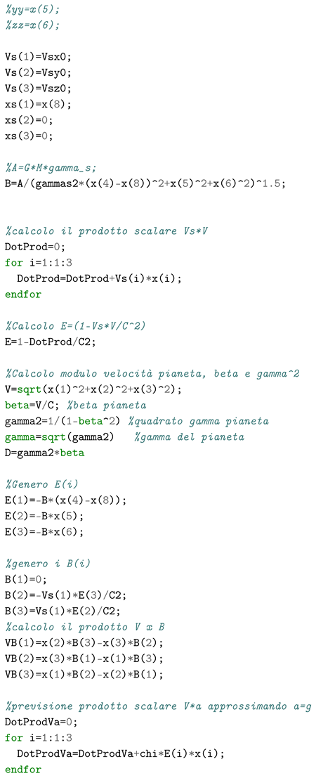
3): we then carried out for each case two limits simulations for each planet: one with the plane of the orbit orthogonal to the speed of the Sun, the other with the speed of the Sun lying in the plane of the orbits. Octave scripts for the latter cases with Sun’s velocity set at 370 km/s are given in the Appendix A and Appendix B
4): the precession manifested in an orbit was calculated as the angle between the radius vector of the planet’s position after a period and that of the aphelion position in the case of the immobile Sun. The total precession in one century was then calculated for both planets and, therefore, the relative precession, i.e. the difference between the precession of Mercury and that of the Earth, which is the one perceived by a stationary observer with respect to the plane of the Earth’s orbit.

The results, referring to a century, are as follows:

A) Velocity of the Sun 220 km/s:

1): plane of the orbit orthogonal to the speed of the sun: relative precession equal to 160 " of degree
2): orbit plane containing the speed of the Sun: relative precession equal to 189 " of degree.

B) Velocity of the Sun 370 km/s:

1): plane of the orbit orthogonal to the speed of the sun: relative precession equal to 452 " of degree
2): orbit plane containing the speed of the Sun: relative precession equal to 751 " of degree.

It is clear that the inclination of the orbit matters as well as the choice of the speed of the Sun.

The precession values obtained are quite greater than the expected one. However, it must be kept in mind that the dominant parameters of the model in this simulation, i.e.

k_{0}^{'}

, the hemicharge of the Sun and the weighted average hemicharge-to-mass ratio of the planets, are unknown at the moment and have been estimated with a very rough approximation.

What we feel we can say now is that the theory provides results compatible with the recognized value in astronomy, above all considering that the total precession of Mercury detected in a century is a good 5600 arc seconds of which nearly 5026 attributed to precession of equinoxes and further 531 as products from various causes such as the influence of other planets, the deformation of the Sun due to its rotation etc., remaining unexplained 43".

Apart from the above, it is interesting to see the contributions given to the acceleration by the various terms that compose it. The table below shows the values of the absolute precession of Mercury in a century, calculated both with the Sun at rest and in motion, in the case of velocity of the Sun lying on the orbit’s plane.

Table 1. Acceleration composition analysis.

Mercury’s absolute precession in a century
Acceleration	Sun’s velocity 0 km/s	Sun’s velocity 370 km/s
$\vec{a} = χ_{p} {\vec{E}}_{n}$	0	220
$\vec{a} = \frac{χ_{p}}{γ} {\vec{E}}_{n}$	9.9	712
$\vec{a} = \frac{χ_{p}}{γ} {\vec{E}}_{n} - γ^{2} β \frac{\vec{a} \cdot \vec{v}}{v c} \vec{v}$	0.8	736
$\vec{a} = \frac{χ_{p}}{γ} ({\vec{E}}_{n} + \vec{v} \times {\vec{B}}_{n}) - γ^{2} β \frac{\vec{a} \cdot \vec{v}}{v c} \vec{v}$	0.8	1468

It is noted that:

1): the impact of the relativistic effect on the electric field generates about 220"
2): the relativistic effect on the mass of the planet, which varies along the orbit due to the variation of the velocity, generates about an additional 500"
3): the impact of the planet’s gamma variation ( $\dot{γ}$ ) is negligible
4): the magnetic force makes an additional contribution of about 720".

7.3. Light Deflection in a Gravitational Field

The momentum of a photon is:

\vec{p} = \frac{ε}{c} \vec{v}

in which

\vec{v}

is the versor of the velocity of the photon.

The equation of motion in the gravitational field of the Sun, here suppose at rest, whose hemicharge is

Q_{s}

, is as follows:

q_{p} {\vec{E}}_{s} = \frac{d \vec{p}}{d t} = \frac{1}{c} (\frac{d ε}{d t} \vec{v} + ε \frac{d \vec{v}}{d t})

(47)

Since it is:

{\vec{E}}_{s} = - k_{0}^{'} \frac{Q_{s}}{r^{2}} \vec{u}

with

\vec{u}

being the versor pointing the photon, the motion equation become:

- k_{0}^{'} \frac{Q_{s} q_{p}}{r^{2}} \vec{u} = \frac{1}{c} (\frac{d ε}{d t} \vec{v} + ε \frac{d \vec{v}}{d t})

Being

q_{p} = χ_{p} ε / c^{2}

with

χ_{p}

from Eq.( 17), the above equation becomes:

- \frac{α e}{m_{e} c^{2}} k_{0}^{'} \frac{Q_{s}}{r^{2}} ε \vec{u} = \frac{1}{c} (\frac{d ε}{d t} \vec{v} + ε \frac{d \vec{v}}{d t})

that after introducing the parameter A defined by:

A = \frac{α k_{0}^{'} e}{m_{e} c^{2}} Q_{s}

becomes:

- A \frac{ε}{r^{2}} \vec{u} = \frac{1}{c} (\frac{d ε}{d t} \vec{v} + ε \frac{d \vec{v}}{d t})

(48)

Now we can suppose to have the Sun at rest with its center in the origin of the reference frame and the photon coming from the left horizontally on a straight line distant from the origin as the Sun’s radius. With this setup, we’ll have that:

\vec{u} = (\frac{x}{r}, \frac{y}{r})

\vec{v} = (cos α, sin α)

being from here on

α

the angle between the positive x axis and the versor

\vec{v}

Now, it is useful to write:

\frac{d ε}{d t} = \frac{d ε}{d x} \frac{d x}{d t} = \frac{d ε}{d x} c \cdot cos α

and similarly, for the versor

\vec{v}

we’ll write:

\frac{d \vec{v}}{d t} = (- c \cdot sin α \frac{d α}{d x}, c \cdot cos α \frac{d α}{d x})

Using the above in the Eq.( 48) and considering its projection on the x and y axes, we obtain the two following equations:

- A \cdot ε \frac{x}{r^{3}} = \frac{d ε}{d x} {cos}^{2} α - ε \cdot sin α cos α \frac{d α}{d x}

(49)

- A \cdot ε \frac{y}{r^{3}} = \frac{d ε}{d x} sin α cos α + ε \cdot {cos}^{2} α \frac{d α}{d x}

(50)

Now we can derive

d ε / d x

from Eq.( 49) and substitute it in Eq.( 50). With some algebra we obtain finally for

α

the following differential equation:

\frac{d α}{d x} = \frac{A}{r^{2}} (u_{x} \cdot tan α - u_{y})

(51)

It is remarkable to note that Eq.( 51) does not more contain explicitly the energy

ε

of the photon nor variables depending on her. That is, the photon trajectory does not depend on its energy.

Now, by completing the equations system with the following:

r = \sqrt{x^{2} + y^{2}}

\frac{d x}{d t} = c \cdot cos α

\frac{d y}{d t} = c \cdot sin α

and the parameters and initial conditions set:

$M_{s} = 1.989 \times 10^{30}$ kg (Sun’s mass)
$χ = 6.4254 \times 10^{8}$ Coulomb/kg
$k_{0}^{'} = 1.6165 \times 10^{- 28}$ $\frac{k g \cdot m^{3}}{C o u l o m b^{2} \cdot s^{2}}$
$Q_{s} = M_{s} χ = 1.2781 \times 10^{39}$ Coulomb (Sun’s hemicharge)
$x (0) = - 7.0 \times 10^{11}$ m (five a.u.)
$y (0) = 6.960 \times 10^{8}$ m (Sun’s radius)
$α (0) = 0$

that provide

A = 2, 950.42

. We have integrated the Eq.( 51) numerically as in the Octave script in Appendix C, with the photon grazing the Sun on a trajectory 10 a.u. long, with the Sun at the midpoint.

We have obtained a deflection of 1.75" of degree, that is the expected value.

8. Antimatter in a Gravitational Field

Here we aim to equip ourselves with the tools to calculate the free fall acceleration of a hemicharged test body q with mass m in the gravitational field on the Earth’s surface.

In particular, we are interested in being able to calculate the ratio between said acceleration and that generically indicated with g, which represents the acceleration of gravity on the Earth’s surface of ordinary or, we could say, average matter. We therefore indicate with g the quantity

g = 9.8066 m / s^{2}

Let

Q_{E}

be the hemicharge of the Earth here and R the Earth’s radius.

The equation (7) giving the gravitational force acting on the test body specializes in:

\vec{F} = - k_{0}^{'} \frac{Q_{E} q}{R^{2}} \vec{u}

(52)

Indicating with

\vec{a}

the acceleration of the test body and applying the second law of dynamics to it, we obtain the following equation:

m \vec{a} = - k_{0}^{'} \frac{Q_{E} q}{R^{2}} \vec{u}

(53)

and for the magnitude of the acceleration:

a = k_{0}^{'} \frac{Q_{E}}{R^{2}} \frac{q}{m}

(54)

Equation (54) can be re-written as:

a = k_{0}^{'} \frac{Q_{E}}{R^{2}} χ

(55)

For the baryonic matter Eq.(55) provides g as follows:

g = k_{0}^{'} \frac{Q_{E}}{R^{2}} χ_{b}

(56)

Where

χ_{b}

is the one already found previously as

α χ_{e}

Therefore, if we want the ratio between the acceleration in free fall of the test body and that of ordinary matter, it is sufficient to divide member by member Eqs.(55) and (56), obtaining:

\frac{a}{g} = \frac{χ}{χ_{b}}

(57)

With the Eq.(57) we are equipped with what is needed to calculate the ratio between the acceleration in free fall of any body compared to that of ordinary matter, on average g.

For each test body it will be sufficient to calculate its hemicharge to mass ratio

χ

and compare it to that of the average ordinary matter

χ_{b}

8.1. Anti-Hydrogen Atom

The anti-hydrogen atom is composed by an anti-proton surrounded by a positron. The hemicharge is the same of that of the hydrogen and the same is also the mass. Therefore, its

χ

is the same as that of hydrogen, which from Fig. 6 already mentioned shows that it is worth

6.431 \cdot 10^{8}

We then get:

\frac{a}{g} = 1.00093

(58)

So, the prediction is that anti-hydrogen falls just like hydrogen, with an acceleration of very little more than g, if not taking also for hydrogen the

χ

adopted in general for the baryonic matter.

8.2. Muonium

Muonium is an exotic and unstable atom, composed only by leptons. In particular, it has an anti-muon, positively charged

+ e

, surrounded by an electron (charge

- e

). The instability is due to that of the anti-muon, which decays with a half-life of

2.1969811 \cdot 10^{- 6} s

Said

m_{μ} = 1.884 \cdot 10^{- 28} k g

the mass of the anti-muon,

m_{p} = 9.109 \cdot 10^{- 31} k g

the mass of the positron,

q = e = 1.6022 \cdot 10^{- 19} C

the hemicharge of the muonium, we have for its hemicharge-to-mass ratio, neglecting the bound energy of the atom:

χ = \frac{q}{m_{μ} + m_{p}} = 8.463 \cdot 10^{8}

(59)

from which we calculate:

\frac{a}{g} = 1.317

(60)

Therefore, the predicted acceleration of the muonium free falling is

32 %

greater than g.

8.3. Positronium

Positronium is a very unstable system composed of a positron and an electron that rotate around the common center of mass. It annihilates into gamma photons in very short times, depending on the state it is, parallel or anti-parallel spins of the particles. Para-positronium lifetime is about

0.124 n s

. In very excited states its mean life can be significantly longer against the annihilation.

The two particles have the same mass and electric charge, in magnitude, those of the electron. Therefore, for its hemicharge-to-mass ratio we have:

χ_{e} = \frac{e}{2 m_{p}} = 8.794 \cdot 10^{10}

(61)

from which we calculate:

\frac{a}{g} = \frac{χ_{e}}{α χ_{e}} = \frac{1}{α} = 137

(62)

Therefore, the predicted acceleration of positronium is very much greater than g.

9. Possible Experimental Tests

The proposed theory establishes the origin of gravity by identifying it in the electric fields, then linking it to the electric charges and to the electric composition of matter, even at the level of the nucleons. Furthermore, as an electromagnetic phenomenon it provides for the magnetism of electrically neutral bodies. It is therefore in these two areas that possible test opportunities should be identified.

Few examples are:

Leptonic matter free fall experiment. As already mentioned, some experiment are under preparation for the positronium and muonium free fall. They will be very critial for the proposed theory. We need to wait for their results.
The case of the free fall of positronium lends itself to a further consideration which we admit is very speculative, but worthy of discussion. Assuming that the measurement highlights a substantial violation of the WEP as predicted by the proposed theory, it would also lend itself to possible further considerations on a hypothetical structure of the electron. In particular, assuming that in another way it was possible to validate the hemicharge-to-mass ratio of the baryonic matter and that it is close to the value estimated here, it would then be possible to calculate the total charge of the electron from the measurement of the acceleration. If it were for example greater than $137 \cdot g$ , then it would be legitimate, at least within this theory, to imagine that the charge $- e$ of the electron is a net value resulting from the sum of two charges, one positive and a negative one, whose net value is precisely $- e$ . In other words, given that $q^{+}$ and $q^{-}$ are the charges constituting the electron such that $q^{+} - q^{-} = - e$ , then the measurement of the acceleration would allow us to calculate $(q^{+} + q^{-}) / 2$ and therefore $q^{+}$ and $q^{-}$ .
Repulsion between parallel moving masses: the theory predicts that bodies or streams of mass running parallel are affected by a repulsive magnetic force. It could be verified whether measurable effects can be observed both at the planetary level (asteroid belt) or at a larger scale at the galactic level, where the revolution speeds of the stars are higher. Or even investigate whether it is possible to observe effects in relativistic jets of matter such as those associated with active galactic nuclei, taking into account the difficulties coming from the intense magnetic field generally acting in those circumstances. But in the case of electrically neutral and non-conducting jets, if observed, the effect could be detectable in the form of a calculable widening of the jet upon the repulsion acting between the constituent particles.
Gravitational waves: the proposed theory predicts that systems composed by massive spinning bodies with high acceleration (e.g. pairs of neutron stars or black holes orbiting each other closely) emit synchrotron radiation, that have peculiar characteristics different from the gravitational waves predicted by the General Relativity. It could be interesting to analyze the data acquired in events such as the one used here for the verification of the peak power during the black holes merger, to search for any characteristic traces of synchroton radiation.
Gravimagnetic effects on space probes which pass close to giant planets such as Jupiter and Saturn: several probes have been launched towards massive planets (Jupiter and Saturn) and the Sun. It would be interesting to verify the presence of anomalies in their trajectories especially near the celestial body, which could be explained as the effect of its gravimagnetic field. The typical effect of helical motion within the gravimagnetic field could be detected, especially if one could eliminate the forces generated by the intense magnetic field of Jupiter or the Sun.

But perhaps also staying closer, investigate the possible gravimagnetic effect on satellites in Earth orbit where, although the gravimagnetic field is lower than the others mentioned, there could be the benefit of the cumulative effect allowed by the long stay in orbit.
Other anomalies of gravitational origin could be observed, if of measurable magnitude, in the trajectories of probes that left the solar system such as the Pioneers and the Voyagers. In this case the gravimagnetic effect would be the one produced by the movement of the sun and the probes with respect to the CMB, for dynamic actions similar to those discussed here in the calculation of the perihelion precession of Mercury.

10. Conclusions

If the proposed theory were to be confirmed, the conclusion would follow that the gravitational interaction does not exist as an autonomous field distinct from the other three interactions recognized in physics. Said in other words, the proposed theory unifies gravitation with electromagnetism stating that the former is only a residual effect of a slight asymmetry between attraction and repulsion, that manifests itself only when the interacting bodies are electrically neutral and the number of pairs of neutral charges is large enough to make emerge the said asymmetry.

The elimination of gravity between the interactions is obviously not a new idea, given that in the theory of General Relativity gravity is a mere consequence of the geometry induced by the momentum-energy tensor. It is therefore evident that the two approaches are radically different and that in our model gravity also manifests gravimagnetic effects in a flat space-time. Therefore, our theory does not need a curved space-time.

As far as the prediction of the phenomena is concerned, at the moment it seems to us that the two theories lead to quite similar results, especially for known experimental cases. The proposed theory foresees many others, some of which are in clear contrast with some commonly established statements such as the UFF. But fortunately, experiments are being prepared for this that will deliver the verdict.

There is also much to be done regarding the general compatibility of the theory with the current knowledge of physics even if, since the theory was built from below basing it on classical electrodynamics, we are quite confident of compliance with the main requirements, many of which already verified by the author.

Preliminary ideas on the areas that remain to be investigated and/or verified are:

1. the projection of the theory in QED. In particular, in the presented theory the graviton is simply a photon emitted by an electrically neutral body. Its modeling in QED and its behavior in that context could be the object of a future work

2. the photon has spin one while the graviton has spin two according to GR. Measurements of the spin of the gravitational waves could give important information about the validity of the theory proposed

3. We have seen that the photon could have a hemicharge-to-mass ratio related to the charge-to-mass ratio of the electron through the fine-structure constant. We are not able to give an explanation of this, but the appearance of such a link between photon and electron in the frame of a gravitational theory seems very fascinating and worthy of further investigation.

And certainly many other things.

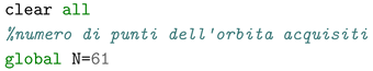
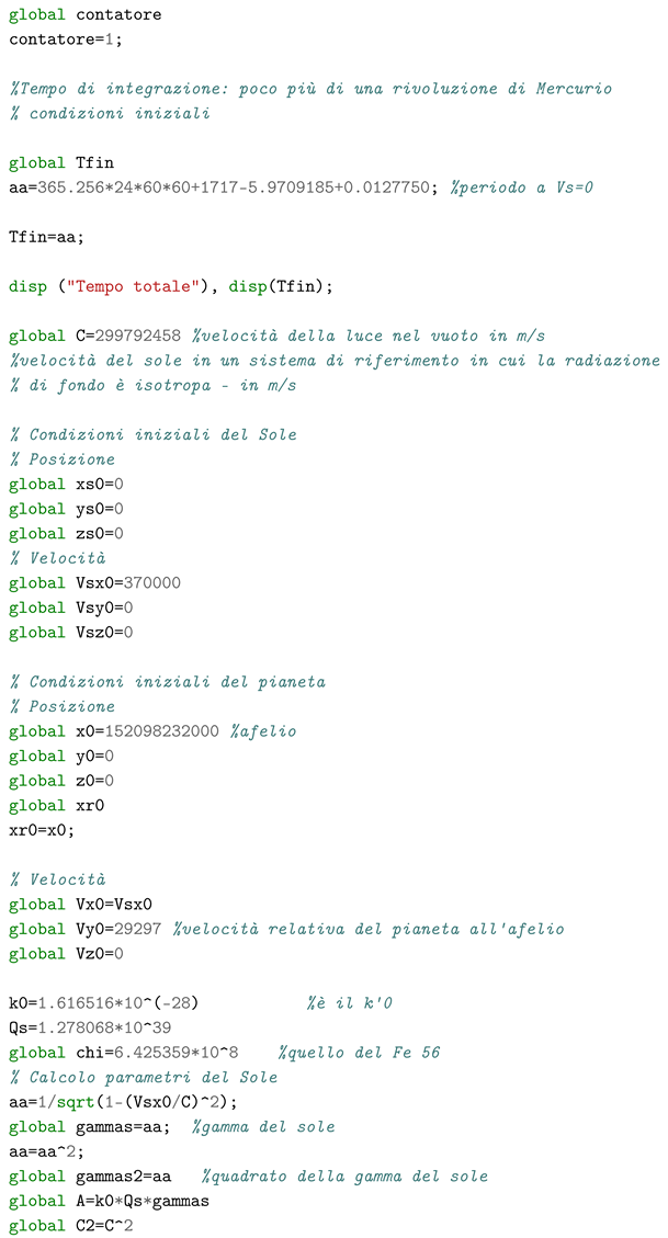
Appendix A. Octave Script for Calculating the Perihelion Precession of Mercury

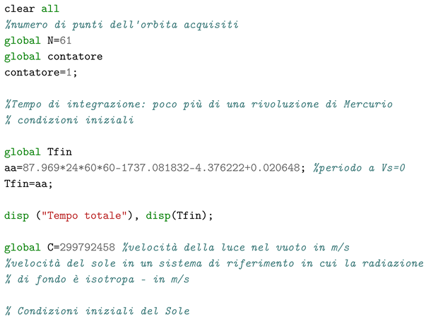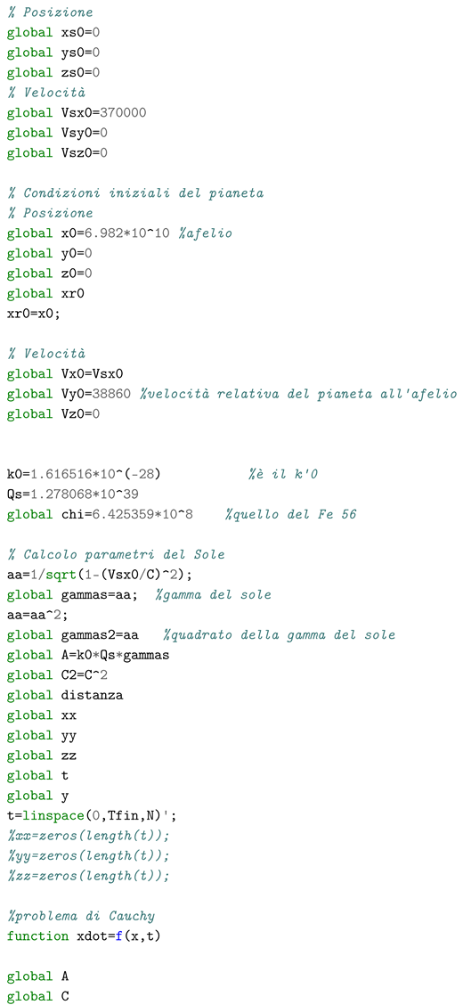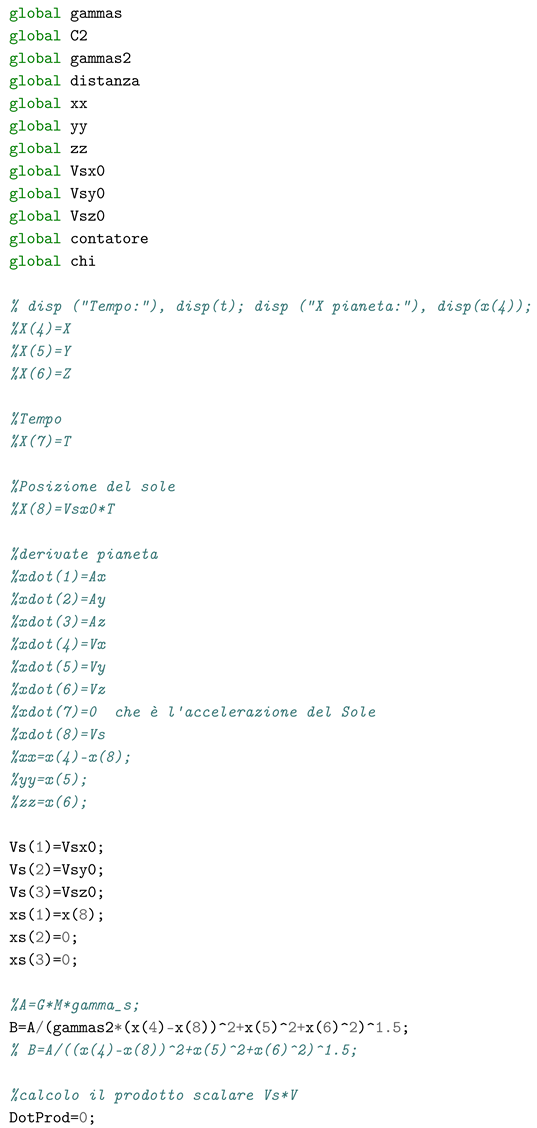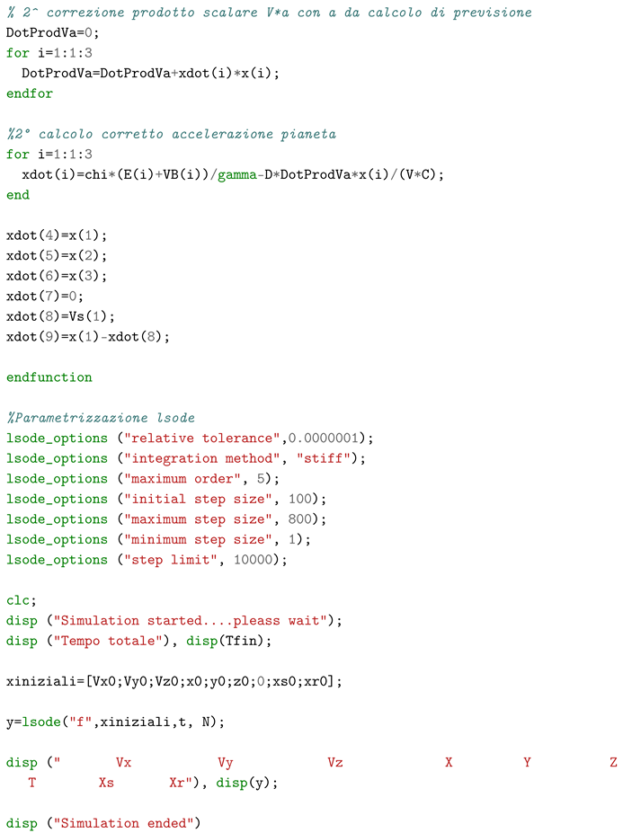Appendix B. Octave Script for Calculating the Perihelion Precession of the Earth

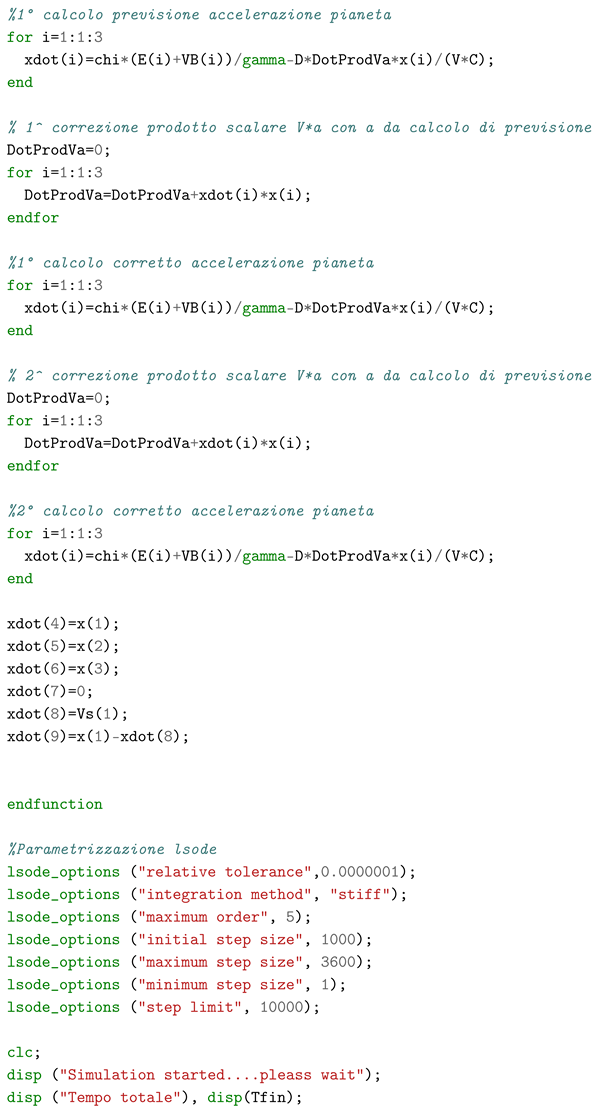Appendix C. Octave Script for Calculating the Light Deflection by the Sun

Appendix D. G’s Measured vs. G’s Calculated

Figure A1. G measured and G calculated for the experiments.

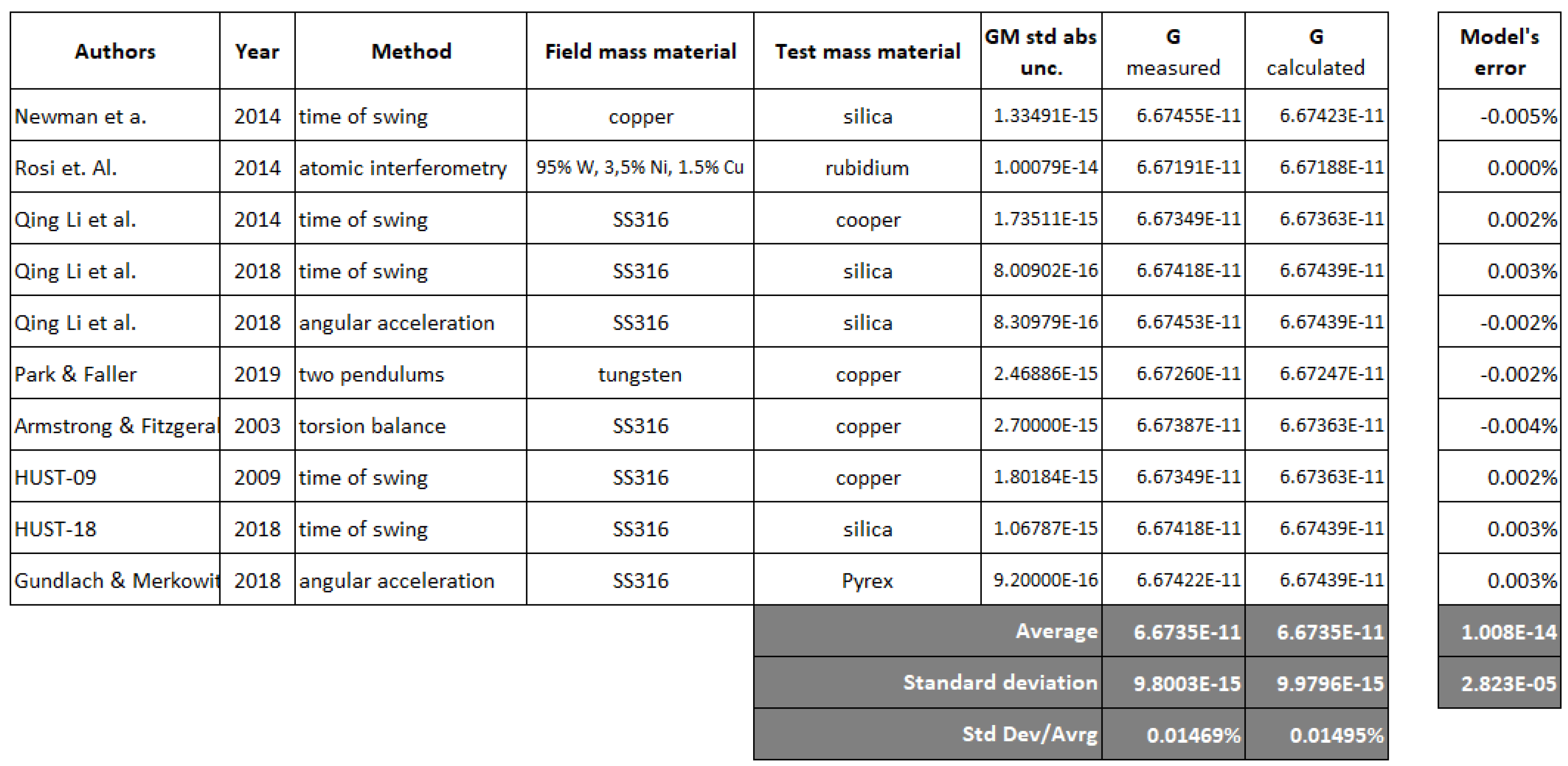
The model’s error is calculated for each experiment using the relevant measured

G_{m}

and calculated

G_{c}

as follows:

E r r o r = \frac{G_{c} - G_{m}}{G_{m}}

Appendix E. Material’s Hemicharges and Signature G’s Calculation

Figure A2. Elements hemicharges and G.

Appendix F. Nucleon’s Partons Structures

Figure A3. Neutron parton’s structure.

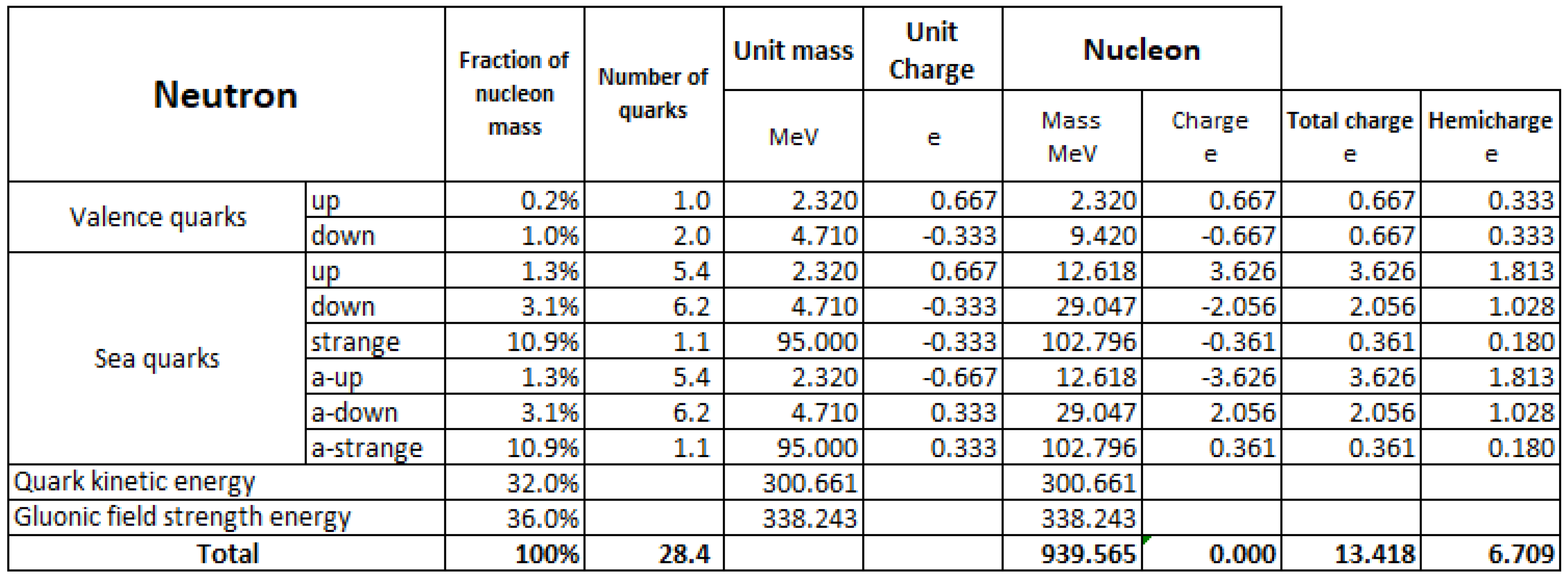
Figure A4. Proton parton’s structure.

Appendix G. GW170814 Merging Black Holes Event

Figure A5. Image credit: B. P. Abbott et al.

References

B.P. Abbott et al., GW170814: "A Three-Detector Observation of Gravitational Waves from a Binary Black Hole Coalescence", PRL 119, 141101 (2017) - LIGO Scientific Collaboration and Virgo Collaboration.
R. Vogt, Nuclear Science Division Lawrence Berkeley National Laboratory Berkeley C, "Physics of the Nucleon Sea Quark Distributions".
Jeremy Darling. Center for Astrophysics and Space Astronomy, Department of Astrophysical and Planetary Sciences, University of Colorado, "The Universe is Brighter in the Direction of Our Motion: Galaxy Counts and Fluxes are Consistent with the CMB Dipole", The Astrophysical Journal Letters, 931:L14 (8pp), 2022 June 1.
Hans W Giertz, Uppsa Research, Miklagard, SE-646 93 Gnesta, Sweden, "The Photon consists of a Positive and a Negative Charge, Measuring Gravity Waves reveals the Nature of Photons".
F. Geesaman - Argonne Associate of Global Empire, LLC, Argonne National Laboratory, Argonne, IL 60439, P. E. Reimer - 0439 2P "The Sea of Quarks and Antiquarks in the Nucleon: a Review".
P. Amaudruz et al. (NMC), “The Gottfried sum from the ratio F2(n) / F2(p),” Phys. Rev. Lett. 66, 2712 (1991).
K. Gottfried, “Sum rule for high-energy electron-proton scattering.” Phys. Rev. Lett. 18, 1174 (1967).
Yi-Bo Yang,1,5 Jian Liang,2 Yu-Jiang Bi,3 Ying Chen,3,4 Terrence Draper,2 Keh-Fei Liu,2 and Zhaofeng Liu3,4 "Proton Mass Decomposition from the QCD Energy Momentum Tensor", Phys. Rev. Lett. 121, 212001 (2018).
C. Rothleitner - Physikalisch-Technische Bundesanstalt (PTB), Bundesallee 100, 38116 Braunschweig, Germany and S. Schlamminger - National Institute of Standards and Technology (NIST), 100 Bureau Drive Stop 8171, Gaithersburg, Maryland 20899, USA and Ostbayerische Technische Hochschule (OTH) Regensburg, Seybothstr. 2, 93053 Regensburg, Germany, "Invited Review Article: Measurements of the Newtonian constant of gravitation, G", Rev. Sci. Instrum. 88, 111101 (2017). [CrossRef]
George T Gillies - Department of Mechanical, Aerospace and Nuclear Engineering, University of Virginia, Charlottesville, Virginia, 22903, USA, "The Newtonian gravitational constant: recent measurements and related studies".
Quinn T, Speake C, Parks H, Davis R. 2014 The BIPM measurements of the Newtonian constant of gravitation, G.Phil. Trans. R. Soc. A 372: 20140032. [CrossRef]
Riley Newman, Michael Bantel, Eric Berg, William Cross- Department of Physics, University of California Irvine, USA, "A measurement of G with a cryogenic torsion pendulum".
G. Rosi, F. Sorrentino, G. M. Tino - Dipartimento di Fisica e Astronomia and LENS Università di Firenze; L. Cacciapuoti - European Space Agency; M. Prevedelli - Dipartimento di Fisica, Universita di Bologna; "Precision Measurement of the Newtonian Gravitational Constant Using Cold Atoms".
Harold V. Parks, James E. Faller - JILA, University of Colorado and National Institute of Standards and Technology "A Simple Pendulum Determination of the Gravitational Constant".
T. Armstrong, M. Fitzgerald "New measurements of G using the measurement standards laboratory torsion balance", PHISYREVLETT.91.201101.
Li Q, Liu J-P, Zhao H-H, Yang S-Q, Tu L-C, Liu Q, Shao C-G, Hu Z-K, Milyukov V, Luo J. 2014 G measurements with time-of-swing method at HUST.Phil. Trans. R. Soc. A 372: 20140141. [CrossRef]
Qing Li, Chao Xue, Jian-Ping Liu, Jun-Fei Wu1, Shan-Qing Yang, Cheng-Gang Shao, Li-Di Quan, Wen-Hai Tan, Liang-Cheng Tu, Qi Liu, Hao Xu, Lin-Xia Liu, Qing-Lan Wang, Zhong-Kun Hu, Ze-Bing Zhou, Peng-Shun Luo, Shu-Chao Wu, Vadim Milyukov & Jun Luo "Measurements of the gravitational constant using two independent methods". [CrossRef]
Jens H. Gundlach and Stephen M. Merkowitz - Department of Physics, Nuclear Physics Laboratory, University of Washington, Seattle, Washington, "Measurement of Newton’s Constant Using a Torsion Balance with Angular Acceleration Feedback".
G. De Toma, "Proposal for a new photon’s model" - 2023.
E. K. Anderson et al., "Observation of the effect of gravity on the motion of antimatter", Nature Vol 621, 28 September 2023.

Disclaimer/Publisher’s Note: The statements, opinions and data contained in all publications are solely those of the individual author(s) and contributor(s) and not of MDPI and/or the editor(s). MDPI and/or the editor(s) disclaim responsibility for any injury to people or property resulting from any ideas, methods, instructions or products referred to in the content.

© 2024 by the author. Licensee MDPI, Basel, Switzerland. This article is an open access article distributed under the terms and conditions of the Creative Commons Attribution (CC BY) license (https://creativecommons.org/licenses/by/4.0/).

Copyright: This open access article is published under a Creative Commons CC BY 4.0 license, which permit the free download, distribution, and reuse, provided that the author and preprint are cited in any reuse.

Downloads

Views

Comments

Subscription

Notify me about updates to this article or when a peer-reviewed version is published.

MDPI Initiatives

Important Links

Choose an area of interest and we will send you notifications of new preprints at your preferred frequency.

Disclaimer

The Roots of Gravity in Electrodynamics the Electrodynamics of Electrically Neutral Bodies

Abstract

Keywords:

Subject:

1. Introduction

2. Electrostatic and Gravitational Fields

2.1. Discussion on Adopting Different Coulomb’s Constants

2.2. Particular Cases

2.3. The Gravitational Field

2.4. Gravitational Potential

2.5. Few Considerations on the Adopted Method

3. The Charge-to-Mass Ratio and Electric Constants Calculation

3.1. Particles

3.2. k 0 ′ Calculation

3.3. The Photon

3.4. New Electric Constants Calculation for Gravity

4. Magnetism from Gravity

4.1. Moving Bodies

4.1.1. Point Particles

4.1.2. Field Generated by a Neutral Mass Current

4.2. Accelerated Bodies

4.2.1. Gravitational Waves

4.2.2. Radiated Power by Accelerating Bodies

4.3. Magnetic Induction by Gravity

5. Lorentz Transformations of the Fields

5.1. The Four-Vector of ρ and j →

5.2. The Lorentz Formula for the Potentials for a Charge Moving with Constant Velocity

5.3. The Fields of a Point Charge with a Constant Velocity

5.4. Motion of a Planet around a Moving Star

6. Maxwell Equations for Gravity

7. Application of the Theory to Some Cases

7.1. Radiated Power of Merging Black Holes

7.2. Mercury’s Perihelion Precession

7.3. Light Deflection in a Gravitational Field

8. Antimatter in a Gravitational Field

8.1. Anti-Hydrogen Atom

8.2. Muonium

8.3. Positronium

9. Possible Experimental Tests

10. Conclusions

Appendix A. Octave Script for Calculating the Perihelion Precession of Mercury

Appendix B. Octave Script for Calculating the Perihelion Precession of the Earth

Appendix C. Octave Script for Calculating the Light Deflection by the Sun

Appendix D. G’s Measured vs. G’s Calculated

Appendix E. Material’s Hemicharges and Signature G’s Calculation

Appendix F. Nucleon’s Partons Structures

Appendix G. GW170814 Merging Black Holes Event

References

MDPI Initiatives

Important Links

Subscribe

3.2. $k_{0}^{'}$ Calculation

5.1. The Four-Vector of $ρ$ and $\vec{j}$