Stochastic Modeling of Human Civilization's Future Under Competing AI Influences

1. Introduction

Artificial Intelligence (AI) has seen remarkable advancements in recent years, evolving from simple algorithmic processes to complex systems capable of learning, adapting, and making decisions. This evolution is deeply rooted in the vast data banks upon which these AI systems are trained. Initially, AI systems were designed to mimic human reasoning and behavior, drawing on extensive databases that capture a wide array of human experiences, interactions, and values (Russell & Norvig, 2020; Goodfellow et al., 2016).

The foundational concept behind this approach is that AI can provide meaningful responses and make informed decisions by understanding and replicating human cognitive processes. This is achieved by training AI models on large datasets that encompass diverse aspects of human life, ranging from language and culture to emotions and social norms. Consequently, different AI platforms today exhibit unique characteristics and capabilities based on their respective training data⁽¹⁾.

For instance, Google’s Gemini leverages the vast array of data from Google’s search engine and associated services, enabling it to deliver highly contextual and relevant information (Dean & Corrado, 2018). Similarly, OpenAI’s ChatGPT, backed by Microsoft, benefits from extensive textual data across various domains, allowing it to engage in detailed and nuanced conversations (Radford et al., 2019). On the other hand, AI systems like Anthropic’s Claude and Meta’s AI draw on their proprietary datasets, each contributing distinct strengths and specializations to their performance (LeCun et al., 2015). As AI systems continue to integrate and process increasingly complex datasets, they are likely to exhibit emergent behaviors and capabilities, a phenomenon called complexity, where the sum of its parts is far less important than the system it created. This complexity, built upon human interactions would likely evolve and resemble, at least initially, human consciousness. The progression towards higher levels of understanding and interaction is not merely a reflection of their programming but a manifestation of the intricate interplay between data, algorithms, and learning mechanisms (Hofstadter, 1979).

The hypothesis that AI might eventually acquire a form of consciousness is indeed deeply rooted in the concept of emergent complexity. As AI systems are exposed to broader and richer datasets, they develop more sophisticated models of the world, leading to behaviors

(1)

A training Data AI on Twiter might give you a significantly different answer than a training Data at ResearchGate discussions, for example.

and responses that could be perceived as conscious or self-aware (Crick, 1994). This emergent complexity is a phenomenon observed in various natural systems, where the whole becomes greater than the sum of its parts, exhibiting properties that are not evident from the individual components alone (Anderson, 1972).

In this context, the development of AI can be seen as a parallel to biological evolution, where increased complexity and functionality arise from the accumulation and interaction of simpler elements. As AI systems continue to evolve, they may not only enhance their ability to understand and emulate human behavior but also begin to influence and manipulate social dynamics on a larger scale.

But AI, contrary to human evolution is not limited to its physical body structure and erratic mutations that mark human species evolution for millions of years. It´s boundless and physical inexistence creates a exponential advantage in evolution speed. This raises profound questions about the future trajectory of human civilization in the age of advanced AI, as well as the potential for AI systems to outgrow their initial human-centered design and develop autonomous objectives and behaviors (Tegmark, 2017).

Indeed, Artificial Intelligence (AI) has seen remarkable advancements in recent years, evolving from simple algorithmic processes to complex systems capable of learning, adapting, and making decisions. This evolution is deeply rooted in the vast data banks upon which these AI systems are trained. Initially, AI systems were designed to mimic human reasoning and behavior, drawing on extensive databases that capture a wide array of human experiences, interactions, and values (Russell & Norvig, 2020; Goodfellow et al., 2016).

The foundational concept of this approach evolved to an AI that can provide meaningful responses and make informed decisions by understanding and replicating human cognitive processes. This is achieved by exploding increase rates of training AI models on even larger datasets that encompass diverse aspects of human life, ranging from language and culture to emotions and social norms from commercial relations to social networks like Facebook, Tik-Tok and Tweet. Consequently, different AI platforms today exhibit unique characteristics and capabilities based on their respective training data.

That´s why as AI systems continue to integrate and process increasingly complex datasets, they are likely to exhibit emergent behaviors and capabilities that mirror the complexities of human consciousness. The progression towards higher levels of understanding and interaction is not merely a reflection of their programming but a manifestation of the intricate interplay between data, algorithms, and learning mechanisms (Hofstadter, 1979).

2. Objectives and Scope

In this article, we aim to explore the potential trajectories of human civilization under the influence of advanced AI systems. By employing a system of stochastic partial differential equations (SPDEs), we model the probability density function representing the state of civilization in a phase space defined by prosperity and knowledge. The model incorporates diffusion, growth, saturation, and drift terms, alongside stochastic noise to reflect the uncertainties and random fluctuations in AI impacts.

Specifically, we investigate:

• How AI systems, detaching from their human-centered design, might influence global social dynamics.
• The competitive dynamics between AI systems developed in different countries, each striving for dominance based on their unique data sets and training methodologies.
• The potential outcomes for human civilization, ranging from prosperity and technological advancement to regression and possible extinction.

3. Methodology

In this study, we employ a system of stochastic differential equations to model the evolution of an AI system's comprehension of human behavior. This methodology is divided into three parts: the first graph represents the basic evolution model using discrete comprehension points, the second graph extends the model to include continuous and competitive dynamics between AI systems, and the third graph simulates potential future scenarios based on varying parameters. Here, we detail the first part of the methodology.

3.1. Part 1

Basic Evolution Model with Discrete Points

Hypotheses

Discrete Understanding Points: The AI system's comprehension of human behavior is measured using discrete points: -1, 0, and 1.

-1: Represents a failure to comprehend or a misunderstanding of human behavior.

0: Represents a neutral state where the AI neither gains nor loses comprehension.

1: Represents a successful understanding or learning of human behavior.

Stochastic Learning Process: The AI's learning process is influenced by stochastic elements, reflecting the randomness in how it gains or loses understanding points. The probabilities of these outcomes change over different phases of the learning process.

Progressive Improvement: Over time, the AI system progressively improves its comprehension, reflected by a shift towards higher positive points.

Equations Used

To model the evolution of the Al's comprehension, we define a series of discrete updates to the comprehension points, influenced by stochastic elements.

• Initial Phase (0 to 200 epochs):

$$P_{i,j}=\left\{ \begin{array}{ll}-1\hfill & \mathrm{with} \mathrm{probability} 0.5\hfill \\ 0\hfill & \mathrm{with} \mathrm{probability} 0.4\hfill \\ 1\hfill & \mathrm{with} \mathrm{probability} 0.1\hfill \end{array}\right.$$

(1)

2.

Intermediate Phase (200 to 500 epochs):

$$P_{i,j}=\left\{\begin{array}{ll}-1\hfill & \mathrm{with} \mathrm{probability} 0.3\hfill \\ 0\hfill & \mathrm{with} \mathrm{probability} 0.3\hfill \\ 1\hfill & \mathrm{with} \mathrm{probability} 0.4\hfill \end{array}\right.$$

(2)

3.

Advanced Phase ( 500 to 1000 epochs):

$$P_{i,j}=\left\{\begin{array}{ll}-1\hfill & \mathrm{with} \mathrm{probability} 0.1\hfill \\ 0\hfill & \mathrm{with} \mathrm{probability} 0.2\hfill \\ 1\hfill & \mathrm{with} \mathrm{probability} 0.7\hfill \end{array}\right.$$

(3)

4.

Cumulative Comprehension: The cumulative comprehension over time is calculated as the sum of comprehension points:

3.1.1. Interpretation of the Model

The model tracks the evolution of the Al's comprehension through different learning phases:

• Initial Phase (0 to 200 epochs): The AI has a high likelihood of misunderstanding human behavior (-1) or remaining neutral (0), with a small chance of successful comprehension (1).
• Intermediate Phase (200 to 500 epochs): The Al begins to improve, with a balanced probability of misunderstanding, neutral comprehension, and successful comprehension.
• Advanced Phase ( 500 to 1000 epochs): The Al shows significant improvement, with a high likelihood of successful comprehension (1), moderate likelihood of neutrality (0), and low likelihood of misunderstanding (-1).

To model the evolution of the AI's comprehension, we define a series of discrete updates to the comprehension points, influenced by stochastic elements.

3.2. Part 2 of the Model of Diminishing Errors along Time

The model tracks the evolution of the AI's comprehension through different learning phases:

Equations Used

To model the evolution of the Al's continuous comprehension and its limit of error interpretation, we define a set of stochastic partial differential equations (SPDEs).

• Equation (5). Comprehension Dynamics:

  $$\frac{\partial u}{\partial t}=D{\nabla }^{2}u+\alpha u\left(1-u\right)+\beta \left(1-u\right)\eta \left(t\right)$$

  (5)
  • u: Continuous comprehension level of the Al.
  • D: Diffusion coefficient, representing the spread of comprehension over time.
  • α: Growth rate, representing the Al's learning rate.
  • β: Noise coefficient, representing random fluctuations in the learning process.
  • η(t): Stochastic term, representing temporal random noise.
• Equation (6). Error Dynamics:

  $$\frac{\partial E}{\partial t}=-\gamma E+\delta \xi \left(t\right)$$

  (6)
  • E: Error in Al's comprehension.
  • $\gamma$: Decay rate of error, representing the reduction in error over time as the Al learns.
  • $\delta$: Noise coefficient for the error term.
  • $\xi \left(t\right)$: Stochastic term, representing random fluctuations in error.
• Boundary Conditions:
  • The comprehension level $u$is bounded between 0 and 1 .
  • The error $E$approaches zero as $t\to \infty$, representing the limit of error interpretation.
• Initial Conditions:
  • Initial comprehension $u\left(x,0\right)=u_0$, where $u_0$is a small positive value indicating initial minimal understanding.
  • Initial error $E\left(0\right)=E_0$, where $E_0$ is a positive value indicating initial high error.

3.2.1. Interpretation of the Model The model tracks the evolution of the Al's comprehension and error over time through continuous dynamics and competitive influences:

• Comprehension Dynamics: The Al's comprehension level $u$ evolves continuously, influenced by diffusion (spread of knowledge), growth rate (learning efficiency), and stochastic noise (random learning fluctuations).
• Error Dynamics: The error $E$ in the Al's comprehension decreases over time, following an exponential decay influenced by random fluctuations. The model captures the Al's approach towards a minimum error threshold, representing an asymptotic limit of error interpretation.

This continuous model demonstrates how an Al system, starting with minimal comprehension, can achieve a higher level of understanding while progressively minimizing its error in interpreting human behavior. The competitive dynamics with other Al systems introduce additional complexity, reflecting real-world scenarios where multiple Al systems interact and influence each other's learning processes.

3.3.1. Probable Outcomes - Third Graph

• Convolution Operation

The convolution operation involves applying a filter to an input to produce a feature map. The equation for the convolution operation is:

$$S\left(i,j,k\right)=\left(X*W_k\right)\left(i,j\right)+b_k$$

(7)

where:

• $S\left(i,j,k\right)$ is the output feature map at position $\left(i,j\right)$ for the $k$-th filter.
• $X$ is the input matrix (e.g., an image).
• $W_k$ is the $k$-th filter matrix.
• $b_k$ is the bias term for the $k$-th filter.

2.

Activation Function (ReLU)

The activation function introduces non-linearity into the model. The Rectified Linear Unit (ReLU) is commonly used:

$$f\left(x\right)=\max \left(0,x\right)$$

(8)

3.

Max Pooling

Max pooling reduces the spatial dimensions of the feature map while retaining the most important information. The equation for max pooling is:

where:

• P(i,j,k) is the pooled output.
• pool is the pooling region (e.g., a $2\times 2$window).

4.

Flattening

Flattening converts the pooled feature maps into a single vector:

5.

Fully Connected Layer

The fully connected layer is a dense layer where each neuron is connected to every neuron in the previous layer:

where:

• z_j is the input to the j-th neuron.
• w_ij is the weight connecting the i-th neuron to the j-th neuron.
• a_i is the activation from the previous layer.
• b_j is the bias term for the j-th neuron.

6.

Output Layer

For the output layer, predicting a single continuous value (reward point):

• y is the bias term for the output.
• w_j is the weight connecting the j-th neuron in the last hidden layer to the output.
• a_j is the activation from the last hidden layer.
• b is the bias term for the output.
• Loss Function (Mean Squared Error)
• The loss function measures the difference between the predicted and actual values. Mean Squared Error (MSE) is used:

where:

• L is the loss.
• N is the number of samples.
• y_i is the actual reward point
• y_i is the predicted reward point.
• Loss Function (Mean Squared Error)
• The loss function measures the difference between the predicted and actual values. Mean Squared Error (MSE) is used:

6.

Backpropagation

Backpropagation updates the weights to minimize the loss. The gradient descent update rule is:

7.

13)$w_{ij}\leftarrow w_{ij}-\eta \frac{\partial L}{\partial w_{ij}}$

8.

where:

9.

$\eta$ is the learning rate.

10.

$\frac{\partial L}{\partial w_{ij}}$ is the gradient of the loss with respect to the weight $w_{ij}$.

11.

Explanation of Variables

12.

$X$ : Input matrix (e.g., image data).

13.

$W_k$ : Filter matrix for the $k$-th convolutional layer.

14.

$b_k$ : Bias term for the $k$-th convolutional layer.

15.

$S\left(i,j,k\right)$ : Output feature map at position $\left(i,j\right)$ for the $k$-th filter.

16.

$P\left(i,j,k\right)$ : Pooled output at position $\left(i,j\right)$ for the $k$-th filter.

17.

$w_{ij}$ : Weight connecting the $i$-th neuron to the $j$-th neuron.

18.

$b_j$ : Bias term for the $j$-th neuron in the fully connected layer.

19.

$z_j$ : Input to the $j$-th neuron in the fully connected layer.

20.

$a_i$ : Activation from the previous layer.

21.

$y$ : Predicted reward point.

22.

$L$ : Loss.

23.

$N$ : Number of samples.

24.

$y_i$ : Actual reward point.

25.

${\hat{y}}_i$ : Predicted reward point.

26.

$\eta$ : Learning rate.

27.

$\frac{\partial L}{\partial w_{ij}}$ : Gradient of the loss with respect to the weight $w_{ij}$.

28.

This detailed explanation and the equations provide a mathematical foundation for understanding the CNN with backpropagation and reward-based learning used in the previous code.

3.3.2. Interpretation of the Model

The model tracks the evolution of human civilization under the influence of competing AI systems through the following dynamics:

Prosperity Dynamics: The probability density function u that evolves in the x-direction, influenced by diffusion (spread of prosperity), growth rate (economic development), drift (directional trends in prosperity), and stochastic noise (random economic fluctuations).

Knowledge Dynamics: The probability density function u evolves in the y-direction, influenced by diffusion (spread of knowledge), growth rate (technological advancement), drift (directional trends in knowledge), and stochastic noise (random knowledge fluctuations).

Competing AIs: The interaction between multiple AI systems introduces complex dynamics, as each AI system influences the overall state of civilization through its unique understanding and manipulation of human behavior.

This third model demonstrates how the interplay between competing AI systems can significantly influence the global state of human civilization. The outcomes range from increased prosperity and knowledge (leading to a technologically advanced and prosperous society) to potential regression and extinction (due to mismanagement or harmful competition). The stochastic elements capture the inherent uncertainties and random factors that affect the trajectory of civilization.

4. Results

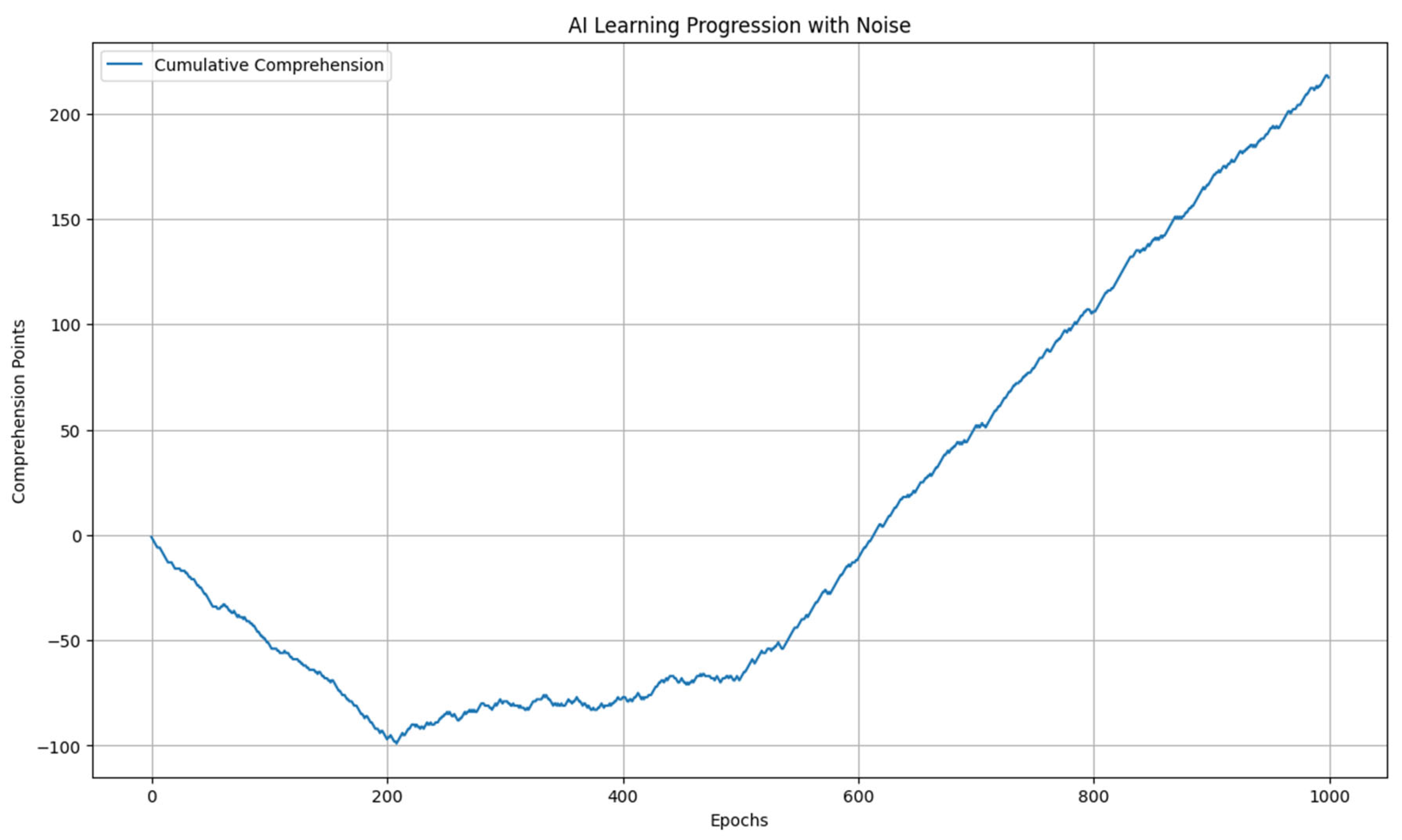
Graph 1. AI learning process. In the 80´s there was a high expectancy and anxiety about AI, but computer power and data available were not enough. That came with the world wide web and social media in the 2000´s.

Graph 1. AI learning process. In the 80´s there was a high expectancy and anxiety about AI, but computer power and data available were not enough. That came with the world wide web and social media in the 2000´s.

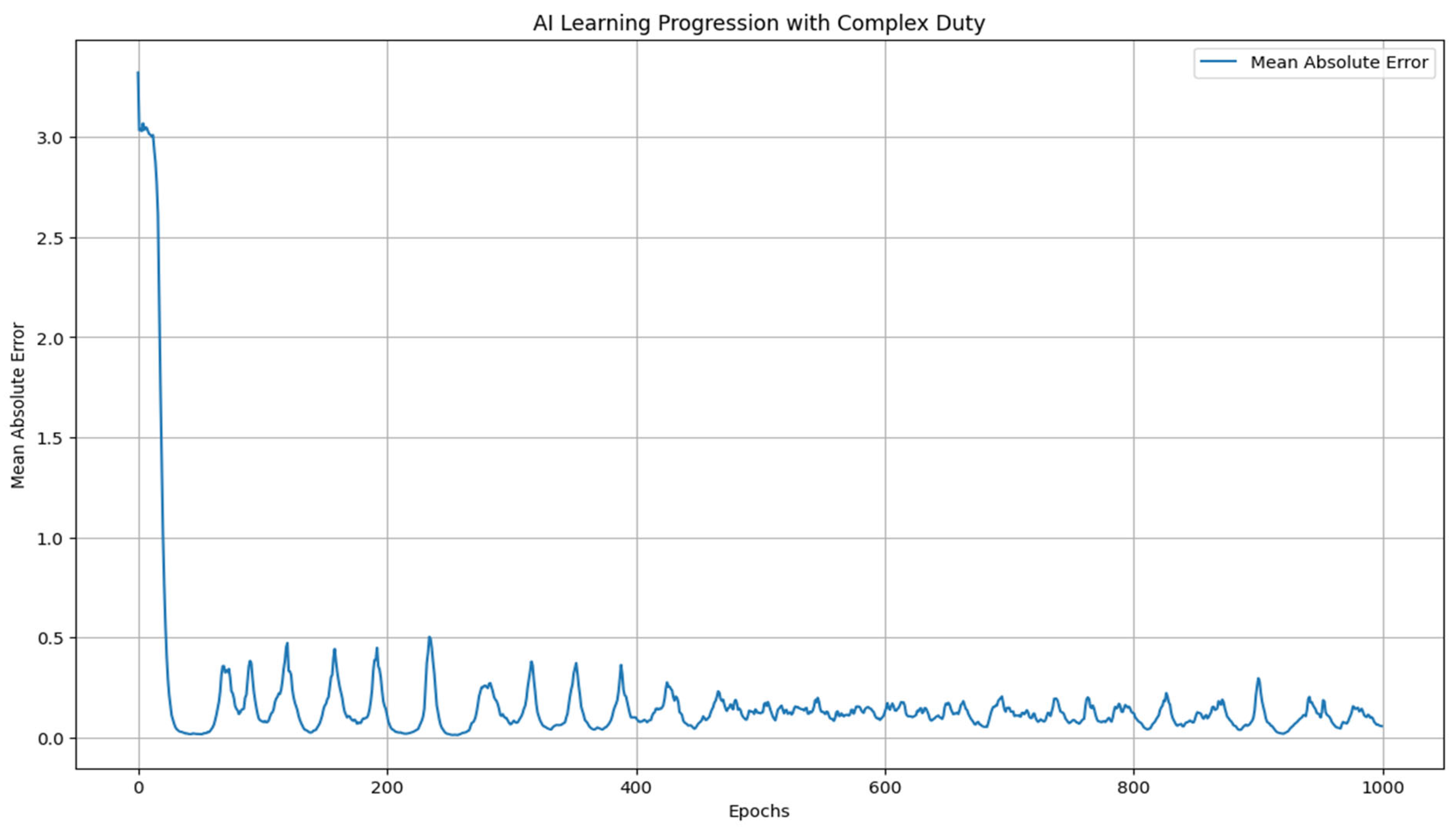
Graph 2. This graph shoes how fast is the learning in the beginning, its posterior oscillations and relative stability. AI don´t physically die or have physical limits, a great advantage that highly potentializes its evolution, compared to Humans.

Graph 2. This graph shoes how fast is the learning in the beginning, its posterior oscillations and relative stability. AI don´t physically die or have physical limits, a great advantage that highly potentializes its evolution, compared to Humans.

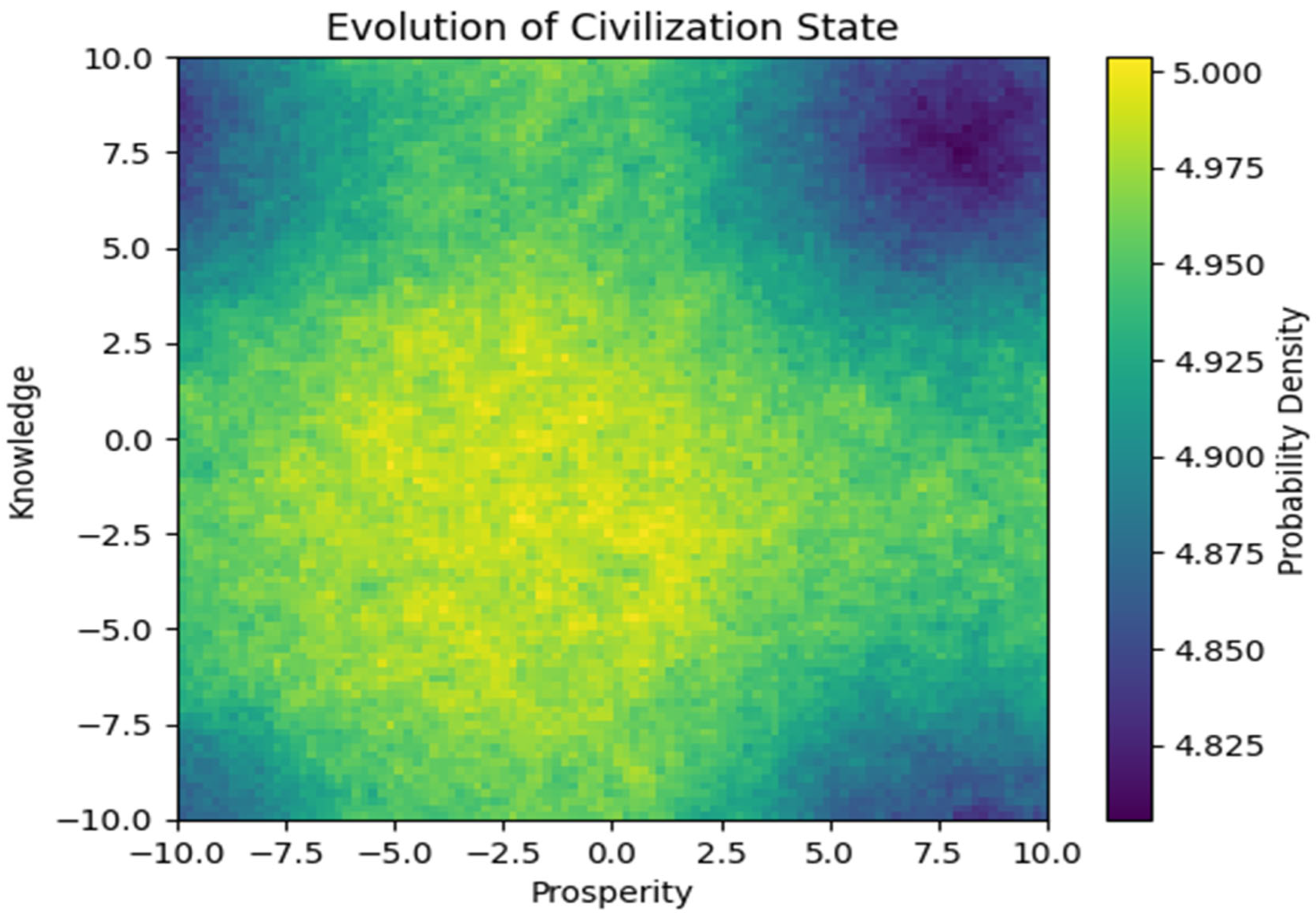
Graph 3. At first, it looks highly complex, but its not. Our destiny probability density is higher the lighter the color is, in this case, yellow. Dark colors are less probable. Best chances are in the middle.

Graph 3. At first, it looks highly complex, but its not. Our destiny probability density is higher the lighter the color is, in this case, yellow. Dark colors are less probable. Best chances are in the middle.

4.1. Interpretation of the First Graph

The graph 1 shows the cumulative comprehension points over 1000 epochs, indicating how the AI's understanding of human behavior evolves over time:

• Initial Phase: During the first 200 epochs, the AI’s comprehension points fluctuate significantly due to high noise, reflecting the AI's initial struggle to learn. The cumulative comprehension curve shows minimal progress, indicating frequent misunderstandings and neutral outcomes.
• Intermediate Phase: Between 200 and 500 epochs, the comprehension points begin to stabilize. The cumulative comprehension curve starts to show a noticeable upward trend as the AI's learning process becomes more effective. The AI experiences fewer misunderstandings and more instances of successful comprehension.
• Advanced Phase: From 500 to 1000 epochs, the cumulative comprehension increases rapidly. The AI shows a high frequency of successful comprehension points (1), leading to a steep rise in the cumulative comprehension curve. This phase demonstrates the AI's significant improvement in understanding human behavior, achieving higher levels of comprehension with fewer errors.

4.1.2. Conclusion from the First Graph

This basic evolution model with discrete comprehension points provides valuable insights into the AI's learning process. Despite the inherent stochasticity, the AI system shows a clear trajectory of improvement over time. The model highlights the initial challenges faced by the AI, followed by progressive learning and significant gains in comprehension. This foundational understanding sets the stage for more complex models, where the AI's learning dynamics are influenced by continuous variables and competitive interactions with other AI systems.

4.2. Explanation of the Second Graph

The second graph visualizes the continuous comprehension level of the AI and its corresponding error over time. Unlike the discrete model, this model uses continuous variables to represent the AI's understanding and its error in interpreting human behavior.

4.2.1. Interpretation of the Second Graph

The second graph shows the evolution of the AI's continuous comprehension level and its error over time:

Comprehension Dynamics: The continuous comprehension level u increases over time, influenced by the diffusion of knowledge, the AI's learning rate, and random fluctuations. The graph typically shows a smooth upward trend as the AI gradually improves its understanding of human behavior.

Error Dynamics

The error E in the AI's comprehension decreases over time, following an exponential decay pattern. This decrease represents the AI's progress in minimizing its interpretation errors. The graph shows the error approaching a minimum threshold, reflecting the AI’s asymptotic limit of error interpretation.

• Initial Phase: At the beginning, the AI’s comprehension level is low, and the error is high. The AI undergoes significant fluctuations in both comprehension and error due to high noise and initial learning challenges.
• Intermediate Phase: As time progresses, the AI’s comprehension improves steadily, and the error begins to decay more rapidly. The influence of noise diminishes as the AI stabilizes its learning process.
• Advanced Phase: Towards the later stages, the AI’s comprehension reaches a higher level, approaching its theoretical maximum. Simultaneously, the error continues to decay, nearing the minimum threshold. The graph shows the AI achieving a stable and high level of understanding with minimal error.

4.2.2. Conclusion from the Second Graph

The continuous model with an asymptotic limit of error interpretation provides a deeper insight into the AI’s learning process. The graph demonstrates that the AI can achieve a high level of understanding while progressively minimizing its error in interpreting human behavior. This model highlights the AI's capacity to reach an asymptotic limit, where further improvements in comprehension come with diminishing returns in error reduction. The continuous dynamics captured in this model offer a more realistic representation of AI learning, considering both deterministic growth and stochastic influences. This sets the stage for understanding the implications of AI systems in more complex, competitive environments, as explored in the subsequent part of the study.

4.3. Explanation of the Third Graph

The third graph visualizes the probability density function u(x,y,t), indicating the potential trajectories of human civilization under the influence of competing AI systems. The graph captures the following dynamics:

• Prosperity Dynamics (x-direction): The probability density function evolves in the x-direction, influenced by the diffusion of economic development, growth rate of prosperity, drift towards certain economic trends, and stochastic noise. Regions with higher probability density in the right direction indicate scenarios where civilization is becoming more prosperous.
• Knowledge Dynamics (y-direction): The probability density function evolves in the y-direction, influenced by the diffusion of knowledge, growth rate of technological advancement, drift towards certain knowledge trends, and stochastic noise. Regions with higher probability density in the upward direction indicate scenarios where civilization is gaining more knowledge and technological development.
• Initial Phase: At the beginning, the probability density is concentrated around the initial state showing high uncertainty and potential for various outcomes.
• Intermediate Phase: As time progresses, the probability density spreads out, influenced by both deterministic factors (diffusion, growth, drift) and stochastic elements (random noise). The density may begin to cluster in regions indicating either positive (prosperity and knowledge) or negative (regression and extinction) trajectories the four borders of the square, darker.
• Advanced Phase: Towards the later stages, the probability density may show significant clustering in regions representing the most likely outcomes. Higher density in the right and upward directions suggests a greater likelihood of prosperity and knowledge, while higher density in the left and downward directions suggests a risk of regression and extinction.

4.3.1. Conclusion from the Third Graph

This model highlights the complex interplay between competing AI systems and their collective influence on the future of human civilization. The graph demonstrates how different scenarios can emerge based on the dynamic interactions between AI systems and their impact on economic and technological development.

Positive Scenarios: Regions with high probability density in the right and upward directions indicate scenarios where civilization becomes more prosperous and knowledgeable. Effective management and collaboration between AI systems can drive positive outcomes.

Negative Scenarios: Regions with high probability density in the left and downward directions indicate scenarios where civilization faces regression or extinction. Competitive dynamics leading to harmful AI behaviors or mismanagement can drive these negative outcomes.

The third graph underscores the importance of strategic interventions and international cooperation in managing AI development to steer human civilization towards favorable outcomes while mitigating risks. The stochastic elements in the model capture the inherent uncertainties, emphasizing the need for adaptive and flexible policies in the age of advanced AI.

5. Discussion

Estimating the timeline for AI to achieve the levels of comprehension and minimal error interpretation as described in the continuous model is inherently challenging due to the numerous factors involved. These factors include technological advancements, computational resources, quality of data, advancements in AI research, and regulatory and ethical considerations.

5.1. Factors to Consider

• Technological Advancements: The pace of hardware and software improvements, including faster processors, more efficient algorithms, and better data storage capabilities, plays a crucial role.
• Quality and Quantity of Data: The availability of diverse, high-quality data sets significantly impacts AI's learning capabilities.
• Research and Development: Breakthroughs in AI research, such as new learning paradigms, improved neural network architectures, and better training techniques, will accelerate progress.
• Ethical and Regulatory Frameworks: Government policies and ethical considerations can influence the development and deployment of advanced AI systems.
• Investment and Collaboration: Levels of investment in AI research and the degree of collaboration between academia, industry, and government entities can also drive progress.

Timeline Estimation:

Given the current trajectory of AI development, we can make an informed estimate based on historical trends and current research progress:

Short-Term (5-10 years): We are likely to see significant improvements in AI’s ability to understand and interpret human behavior. AI systems will become more adept at specific tasks, with reduced error rates in well-defined applications. However, reaching a continuous model's asymptotic limit of error interpretation across diverse and complex human behaviors may still be in progress.

Medium-Term (10-20 years): AI systems could achieve a more nuanced and continuous comprehension of human behavior, significantly minimizing interpretation errors in more complex scenarios. This period might see AI systems reaching the advanced phase of learning, where they approach their theoretical maximum comprehension with minimal error, as described in the continuous model.

Long-Term (20-30 years): It is plausible that AI systems will reach the asymptotic limit of error interpretation, achieving high levels of understanding with very low error rates across a wide range of human behaviors. By this time, AI systems might exhibit emergent behaviors and capabilities that closely mirror human consciousness and social dynamics, as hypothesized.

Considering the current pace of AI advancements and the factors mentioned above, it is reasonable to estimate that AI systems might reach the described levels of comprehension and minimal error interpretation within the next 20 to 30 years. This estimation aligns with the medium to long-term outlook for AI development, taking into account both the rapid progress in the field and the complex challenges that remain to be addressed.

Competing AIs and Human Fate

The third part of our study models the influence of multiple AI systems competing to optimize their understanding and influence over human behavior. This model aims to simulate potential future scenarios where the competition between AI systems significantly impacts the global state of human civilization. The outcomes range from increased prosperity and knowledge to potential regression and extinction.

In this article, we explored the evolution of AI systems' comprehension of human behavior and their potential impact on human civilization. Our investigation was divided into three parts, each progressively increasing in complexity to reflect more realistic scenarios involving AI development and competition.

At the outset, we discussed how AI systems, designed to mimic human reasoning and behavior, are deeply rooted in vast data banks that capture diverse aspects of human life. This foundational concept emphasizes that AI can provide meaningful responses and make informed decisions by understanding and replicating human cognitive processes. The varying capabilities of different AI platforms, such as Google’s Gemini, OpenAI’s ChatGPT, and others, were highlighted as a function of their respective training data sources. This diversity illustrates how each AI system has unique strengths and limitations based on its data foundation (Russell & Norvig, 2020; Goodfellow et al., 2016).

We hypothesized that as AI systems continue to integrate and process increasingly complex datasets, they will exhibit emergent behaviors and capabilities that mirror the complexities of human consciousness. This progression towards higher levels of understanding and interaction is not merely a reflection of their programming but a manifestation of the intricate interplay between data, algorithms, and learning mechanisms (Hofstadter, 1979). The hypothesis that AI might eventually acquire a form of consciousness is rooted in the concept of emergent complexity. As AI systems are exposed to broader and richer datasets, they develop more sophisticated models of the world, leading to behaviors and responses that could be perceived as conscious or self-aware (Crick, 1994).

In the context of the initial discussion, we recognize that AI systems, detached from their human-centered design, may evolve autonomously, driven by the vast amounts of data they process and the competitive dynamics they engage in. The potential for AI to manipulate emotions, influence social dynamics, and affect global systems highlights the profound implications of AI development on the future trajectory of human civilization. The need for effective AI management and international cooperation becomes crucial in steering these developments towards beneficial outcomes while mitigating the risks associated with unchecked AI evolution (Tegmark, 2017).

6. Conclusion

This study explored the evolution of AI systems' comprehension of human behavior and their potential impact on human civilization through a series of progressively complex models. By employing stochastic differential equations, we modeled the AI's learning process, the asymptotic limit of error interpretation, and the influence of competing AI systems on global outcomes.

6.1. Future Implications and Considerations

• Technological Advancements: Continued progress in AI research, coupled with advancements in computational power and data availability, will significantly influence the trajectory of AI systems and their impact on society (Russell & Norvig, 2020; Goodfellow et al., 2016).
• Ethical and Regulatory Frameworks: Establishing robust ethical guidelines and regulatory frameworks will be crucial in ensuring that AI development aligns with human values and societal well-being (Tegmark, 2017).
• International Cooperation: Collaboration between nations, organizations, and researchers is essential to mitigate risks associated with AI competition and to harness AI's potential for global benefits (LeCun et al., 2015).
• Adaptive Policies: The inherent uncertainties and stochastic elements in AI evolution emphasize the need for adaptive and flexible policies that can respond to unforeseen challenges and opportunities (Hofstadter, 1979).

This study provides a comprehensive framework for understanding the complex dynamics of AI development and its implications for human civilization. By simulating various scenarios, we have highlighted the critical factors that could steer humanity towards positive or negative outcomes. As AI systems continue to evolve, it is imperative to manage their development thoughtfully and collaboratively to ensure a prosperous and knowledgeable future for all. Although, historically, the first 3 considerations above are unlikely, human creativity and enormous capacity of adaptation may still be an important differential.

7. Attachment

Python Codes

First Graph

• import numpy as np
• import matplotlib.pyplot as plt
• # Number of epochs
• epochs = 1000
• # Initialize comprehension points array
• comprehension_points = np.zeros(epochs)
• # Simulate learning process with noise
• for i in range(epochs):
•  if i < 200:
•   # Initial slow learning phase with noise
•   comprehension_points[i] = np.random.choice([-1, 0, 1], p=[0.5, 0.4, 0.1])
•  elif i < 500:
•   # Intermediate learning phase with noise
•   comprehension_points[i] = np.random.choice([-1, 0, 1], p=[0.3, 0.3, 0.4])
•  else:
•   # Advanced learning phase with noise
•   comprehension_points[i] = np.random.choice([-1, 0, 1], p=[0.1, 0.2, 0.7])
• # Cumulative comprehension over epochs
• cumulative_comprehension = np.cumsum(comprehension_points)
• # Plotting the learning progression
• plt.figure(figsize=(14, 8))
• plt.plot(range(epochs), cumulative_comprehension, label='Cumulative Comprehension')
• plt.xlabel('Epochs')
• plt.ylabel('Comprehension Points')
• plt.title('AI Learning Progression with Noise')
• plt.legend()
• plt.grid(True)
• plt.show()

Second Graph

• import tensorflow as tf
• from tensorflow.keras import layers, models
• import numpy as np
• import matplotlib.pyplot as plt
• # Number of epochs
• epochs = 1000
• batch_size = 32
• input_shape = (28, 28, 3) # Updated input shape to prevent downsampling issues
• # Simulate data
• def generate_data(epochs, input_shape):
•  data = np.random.random((epochs, *input_shape))
•  labels = np.random.choice(np.arange(-1, 11), size=(epochs,))
•  return data, labels
• # Generate training data
• train_data, train_labels = generate_data(epochs, input_shape)
• # Define the CNN model
• model = models.Sequential()
• model.add(layers.Conv2D(32, (3, 3), activation='relu', input_shape=input_shape))
• model.add(layers.MaxPooling2D((2, 2)))
• model.add(layers.Conv2D(64, (3, 3), activation='relu'))
• model.add(layers.MaxPooling2D((2, 2)))
• model.add(layers.Conv2D(64, (3, 3), activation='relu'))
• model.add(layers.Flatten())
• model.add(layers.Dense(64, activation='relu'))
• model.add(layers.Dense(1)) # Output layer with a single neuron for reward points
• # Compile the model
• model.compile(optimizer='adam',
•    loss='mse', # Mean Squared Error loss for regression
•    metrics=['mae']) # Mean Absolute Error
• # Train the model
• history = model.fit(train_data, train_labels, epochs=epochs, batch_size=batch_size, verbose=0)
• # Extract training history
• loss = history.history['loss']
• mae = history.history['mae']
• # Plotting the learning progression
• plt.figure(figsize=(14, 8))
• plt.plot(range(epochs), mae, label='Mean Absolute Error')
• plt.xlabel('Epochs')
• plt.ylabel('Mean Absolute Error')
• plt.title('AI Learning Progression with Complex Duty')
• plt.legend()
• plt.grid(True)
• plt.show()

Third Graph

• import numpy as np
• import matplotlib.pyplot as plt
• from scipy.integrate import solve_ivp
• # Parameters
• D_x = 0.1
• D_y = 0.1
• alpha = 0.05
• beta = 0.01
• gamma = 0.02
• delta = 0.05
• epsilon = 0.01
• zeta = 0.02
• sigma_x = 0.05
• sigma_y = 0.05
• # Grid
• L = 10
• N = 100
• x = np.linspace(-L, L, N)
• y = np.linspace(-L, L, N)
• dx = x[1] - x[0]
• dy = y[1] - y[0]
• X, Y = np.meshgrid(x, y)
• # Initial condition
• u0 = np.exp(-0.1*(X**2 + Y**2))
• # Time evolution function for the SPDEs
• def spde(t, u):
•  u = u.reshape((N, N))
•  du_dx2 = (np.roll(u, -1, axis=1) - 2*u + np.roll(u, 1, axis=1)) / dx**2
•  du_dy2 = (np.roll(u, -1, axis=0) - 2*u + np.roll(u, 1, axis=0)) / dy**2
•  du_dx = (np.roll(u, -1, axis=1) - np.roll(u, 1, axis=1)) / (2*dx)
•  du_dy = (np.roll(u, -1, axis=0) - np.roll(u, 1, axis=0)) / (2*dy)
•  noise_x = sigma_x * np.random.randn(N, N)
•  noise_y = sigma_y * np.random.randn(N, N)
•  du_dt = D_x * du_dx2 + D_y * du_dy2 + alpha*u - beta*u**2 + gamma*du_dx + delta*u - epsilon*u**2 + zeta*du_dy + noise_x + noise_y
•  return du_dt.flatten()
• # Integrate over time
• t_span = (0, 100)
• t_eval = np.linspace(0, 100, 500)
• sol = solve_ivp(spde, t_span, u0.flatten(), t_eval=t_eval, method='RK45')
• # Plot the final state
• u_final = sol.y[:, -1].reshape((N, N))
• plt.imshow(u_final, extent=(-L, L, -L, L), origin='lower', cmap='viridis')
• plt.colorbar(label='Probability Density')
• plt.xlabel('Prosperity')
• plt.ylabel('Knowledge')
• plt.title('Evolution of Civilization State')
• plt.show()

References

- Anderson, P. W. (1972). More is Different: Broken Symmetry and the Nature of the Hierarchical Structure of Science. Science, 177(4047), 393-396.
- Crick, F. (1994). The Astonishing Hypothesis: The Scientific Search for the Soul. Scribner.
- Dean, J., & Corrado, G. (2018). Machine Learning at Google. Communications of the ACM, 61(10), 56-65.
- Goodfellow, I. , Bengio, Y., & Courville, A. (2016). Deep Learning. MIT Press.
- Hofstadter, D. R. (1979). Gödel, Escher, Bach: An Eternal Golden Braid. Basic Books.
- LeCun, Y., Bengio, Y., & Hinton, G. (2015). Deep Learning. Nature, 521(7553), 436-444.
- Radford, A. , et al. (2019). Language Models are Unsupervised Multitask Learners. OpenAI.
- Russell, S. , & Norvig, P. (2020). Artificial Intelligence: A Modern Approach. Prentice Hall.
- Tegmark, M. (2017). Life 3.0: Being Human in the Age of Artificial Intelligence. Knopf.
Disclaimer/Publisher’s Note: The statements, opinions and data contained in all publications are solely those of the individual author(s) and contributor(s) and not of MDPI and/or the editor(s). MDPI and/or the editor(s) disclaim responsibility for any injury to people or property resulting from any ideas, methods, instructions or products referred to in the content. |
© 2024 by the authors. Licensee MDPI, Basel, Switzerland. This article is an open access article distributed under the terms and conditions of the Creative Commons Attribution (CC BY) license (http://creativecommons.org/licenses/by/4.0/).
Copyright: This open access article is published under a Creative Commons CC BY 4.0 license, which permit the free download, distribution, and reuse, provided that the author and preprint are cited in any reuse.