

Submitted:
16 June 2024
Posted:
17 June 2024
You are already at the latest version
Abstract
Nuclear energy, along with renewable and alternative energy sources, is a crucial green energy source. However, the existing literature often overlooks the role of nuclear energy in achieving sustainable development goals. This study analyzes the impact of green technological innovation, nuclear energy consumption, and trade openness on environmental quality in the US, which consumed the most nuclear energy from 1990 to 2019. The ARDL bounds testing approach was applied for its effectiveness in smaller samples, suitable for the data set used in this study, to determine cointegration relationships. Additionally, the Toda-Yamamoto causality test was employed to explore causal links without requiring series stationarity or cointegration. The ARDL cointegration results indicate a significant long-term relationship between CO2 emissions, green technological innovation, nuclear energy consumption, and trade openness. The results suggest that promoting green technological innovation and nuclear energy (although this effect is less certain) can be effective strategies for reducing CO2 emissions, while the impact of trade openness requires careful consideration due to its potential to increase emissions. Green technological innovation has a significant unidirectional causal effect on CO2 emissions. These results will help policymakers design policies to achieve sustainable environmental goals in the US economy.
Keywords:
nuclear energy consumption
; green technological innovation
; environment
; trade openness
; the United States
1. Introduction
The global warming induced by the increase in CO2 emissions (CE) at the global level poses serious challenges in terms of environmental sustainability (ES). According to statistics from the EIA, the increase in global CE has reached approximately 64% between 1990 and 2019, and it is projected to exceed 45% compared to the year 2000 by 2030. The primary cause of this increase is attributed to the heavy reliance of developing countries on fossil-based energy sources [1]. One of the most effective strategies in combating global climate change (GCC) involves the utilization of cleaner energy sources that can serve as alternatives to fossil-based energy, particularly in electricity generation. Renewable energy (RE) and nuclear energy (NE) are prominently featured among these cleaner energy sources. NE is a significant non-carbonizing energy source capable of generating electricity within global energy production systems [2]. The challenge of global warming and GCC urges nations to transition from fossil-based energy towards electricity generation from cleaner energy sources. In this regard, NE holds significant importance for policymakers [3]. This is because NE not only contributes to the reduction of CE [4] but also facilitates economic growth by enabling electricity generation at lower costs [5,6].
The Paris Agreement, adopted on December 12, 2015 during the COP21, is an international agreement legally binding on 196 countries that came into effect on November 4, 2016, addressing GCC. This agreement continues efforts to limit the global average temperature increase to 1.5 °C. To achieve this target, CE must peak no later than 2025 and be reduced by 43% by 2030. Although significant increases in GCC action are needed to meet the goals of this agreement, since it entered into force, an increase has been setting carbon neutrality targets. Zero-carbon solutions are becoming competitive in sectors representing more than 70% of global emissions by 2030. This trend is particularly evident in the energy and transportation sectors, creating numerous new business opportunities for early adopters. Although the United States officially joined the agreement upon its entry into force, it withdrew from the agreement in 2020 following the rejection by the relevant government in 2017. Subsequently, the US officially rejoined the Paris Agreement in 2021 under the decision of the relevant minister, positioning the country once again as part of the global climate solution. Therefore, fulfilling the US’ commitments under the Paris Agreement necessitates prioritizing not only RE sources but also alternative energy sources such as NE.
Nuclear energy consumption (NEC) is a critical metric for understanding the global landscape of energy production and consumption. In 2022, various countries exhibited significant levels of NEC, highlighting their reliance on nuclear power for their energy needs. According to Statista data, the United States leads the world in nuclear energy consumption, utilizing a total of 7.31 exajoules. Following the United States, China and France are the next largest consumers, with China consuming 3.76 exajoules and France 2.65 exajoules. The substantial gap between the United States and other countries underscores its significant investment and dependency on nuclear energy. The data, as illustrated in Figure 1, provides a clear comparison of nuclear energy consumption across leading nations.
The rankings continue with Russia consuming 2.00 exajoules, South Korea 1.59 exajoules, and Canada at 0.78 exajoules. These figures reflect the broader trends in energy policy and infrastructure investment in each country. Additionally, countries like Ukraine, Spain, Japan, and Sweden also contribute significantly to the global nuclear energy landscape, each with consumption levels ranging from 0.56 to 0.46 exajoules.
The United States has a significant infrastructure for nuclear energy, with data from the Energy Information Administration (EIA) indicating that as of August 1, 2023, the country operates 54 commercial nuclear power plants. These plants house a total of 93 nuclear reactors distributed across 28 states. Efforts to increase capacity in these plants have ensured that the entire fleet of operational nuclear reactors maintains high capacity utilization rates. This high efficiency has been a key factor in nuclear energy contributing approximately 19-20% of the total annual electricity generation in the U.S. from 1990 to 2021.
Understanding the trends in nuclear energy production capacity and actual generation is crucial for comprehending the role of nuclear power in the US energy mix. Figure 2 illustrates the nuclear electricity production capacity and output in the US from 2000 to 2022. This figure clearly shows that nuclear energy production has consistently exceeded the capacity for nuclear energy production during this period.
The data presented in Figure 2 highlights the stability and efficiency of nuclear energy production in the US. Over the years, capacity has seen slight fluctuations, but overall generation has remained robust, with slight year-to-year variations. Notably, the use of NE serves as a potential driver for environmental considerations. Guo et al. [7] assert in the literature that NE efficiency reduces CE. Similarly, Lin and Ullah [8] suggest that NE significantly improves environmental quality (EQ). Additionally, numerous studies in the literature reach similar conclusions [2,9,10,11,12,13,14].
About the above results, this study aims to develop a sustainable solution for reducing CE by investigating the connection between NE and the environment for the significant potential of the US economy for the period 1990-2019. The potential contribution of this study is threefold: (i) Although previous literature has investigated the effect of NE on ES, this study is the first to estimate this relationship in the context of GTI and TO using the example of the US, which ranks first in NEC. (ii) Secondly, the study not only focuses on NE usage but also addresses the potential roles of GTI and TO in improving EQ. (iii) Furthermore, the study provides recommendations to policymakers for fulfilling the US’ commitments in the Paris Agreement by identifying the impact of NE on CE. (iv) Additionally, the findings of the study are important in the regulation of future GTI strategies and energy policies. A better understanding of the effects of NEC, GTI, and TO on EQ could assist in directing environmental protection and sustainable development efforts more effectively.
The other parts of the research are structured as follows: Section 2 presents relevant literature regarding the variables included in the ES model. Section 3 outlines the model and methodology employed. Section 4 details predictions concerning the findings and discussion. The study ends with the conclusion and policy recommendations provided in Section 5.
2. Literature Review
2.1. Green Innovation and Environment
In the past decade, technological advancements have significantly impacted various economic sectors worldwide. Consequently, researchers are increasingly investigating how green technology innovation (GTI) influences ecological systems. GTI is seen as a key strategy to combat global environmental problems and achieve sustainable development goals [15,16,17,18,19,20]. Moreover, Hart and Dowell [21] argue that GTI can give companies a competitive edge while benefiting the environment. Recent studies further support that GTI improves environmental quality [22,23,24]. In other words, GTI helps increase production capacities and reduce environmental degradation [17,25,26,27,28,29]. However, some researchers, such as Shao et al. [30], suggest that GTI can reduce carbon emissions in the long run.
Contrary to the positive effects noted, some studies find that GTI might increase carbon emissions due to the “rebound effect” and “green paradox” Fernández et al., [31], Dauda et al. [32], and Rennings, Rammer [33] argue that markets alone don’t promote GTI effectively, emphasizing the need for incentives or regulations to encourage firms to adopt GTI. Additionally, Mongo et al. [34] add that as GTI progresses, both production and energy consumption rise, potentially increasing emissions. Conversely, other studies indicate that GTI has no significant impact on environmental quality. These findings are often linked to countries’ income and development levels [35,36,37,38]. The impact of GTI appears to vary over time and depends on factors such as pollution and income levels [39]. Research results demonstrate that the effect of GTI is stronger in high-income countries [40,41,42]. Furthermore, GTI effectively reduces emissions when they are high [43,44].
2.2. Nuclear Energy and Environment
Nuclear energy is seen as a key player in reducing the negative impact of global energy consumption on the environment by improving energy efficiency worldwide [2,11,13,45,46,47,48]. NE, due to its low-carbon nature, impacts the environment less than renewable energy sources and helps conserve natural uranium resources [49]. This potential for reducing environmental damage has caught the attention of policymakers globally. Supporting this perspective, Cakar et al. [50] found that modern nuclear power plants enhance energy efficiency and environmental health by lowering greenhouse gas emissions through innovation. Many studies agree that NE serves as a temporary low-carbon energy source that helps cut carbon emissions from burning fossil fuels [13,51,52,53,54,55].
However, it is important to consider the contrasting views of some researchers. Sarkodie and Adams [56] and Mahmood et al. [57] argue that NE negatively impacts environmental quality. Similarly, Sadiq et al. [16] found that NE harms environmental sustainability. These studies suggest that issues like radioactive waste, operational inefficiencies, and global nuclear waste management restrictions could increase carbon emissions from NE. Adding to the complexity, Saidi and Mbarek [58] found NE ineffective in preserving environmental quality, and Kartal [59] found no significant impact of NE on carbon emissions. Consequently, these conflicting findings indicate the need for further research to understand the ecological issues and the impact of NE on reducing carbon emissions in the US economy.
2.3. Trade Openness and Environment
Studies on this subject have highlighted four main hypotheses: (1) Promotion hypothesis, (2) Inhibition hypothesis, (3) Feedback hypothesis, and (4) Neutral hypothesis. According to the Promotion hypothesis, increasing trade openness promotes environmental quality. This hypothesis argues that TO facilitates the dissemination of environmental technologies and practices by stimulating economic growth and welfare. Conversely, the Inhibition hypothesis suggests that TO increases environmental degradation (ED). An increase in TO may lead to increased production and depletion of resources, thus escalating environmental pollution (EP). Furthermore, the Feedback hypothesis suggests a mutual interaction between TO and environmental variables. In other words, as TO increases, it affects environmental variables, while the state of environmental variables also influences TO. Finally, the Neutral hypothesis posits that there is no relationship between TO and environmental variables or that the relationship is uncertain.
Empirical studies provide mixed results on these hypotheses. For example, Zamil et al. [60] demonstrated a positive relationship between TO and carbon emissions in Oman, supporting the Inhibition hypothesis. Similarly, Musah et al. [61] found that TO increases ED for D8 countries, while Gozgor [62] and Jun et al. [63] reported similar results for OECD countries and China, respectively. In fact, these findings also align with the Inhibition hypothesis. On the other hand, some studies support the Promotion hypothesis. Chebbi et al. [64], Shahbaz et al. [65], Zhang et al. [66], and Mutascu and Sokic [67] found that TO could significantly reduce the growth of energy pollutants and thus enhance EQ. Similarly, Shahzad et al. [68], Mahmood et al. [3], and Sun et al. [69] determined that TO increases EQ, consistent with the Promotion hypothesis. Additionally, some research aligns with the Neutral hypothesis. Mutascu [70] found a nonsignificant relationship between TO and CE, suggesting no clear link between these variables. As mentioned, the literature presents mixed findings, with different studies supporting different hypotheses. Therefore, additional research is required to clarify the conflicting results regarding the relationship between CE and TO.
To summarize the literature review in three areas related to the model, theoretical and empirical studies highlight GTI as a critical strategy for improving environmental quality and achieving sustainability goals, though some note potential negative effects like the “rebound effect.” NE is recognized for its low-carbon benefits and potential to reduce emissions, though concerns about radioactive waste and operational inefficiencies persist. TO’s impact on the environment is debated through four hypotheses—promotion, inhibition, feedback, and neutral—with mixed empirical support, indicating the need for further research to clarify these relationships.
3. Methods
This study examines the effects of GTI, NEC, and TO on EQ within the context of the US economy, which leads globally in NEC. The dataset includes 30 annual observations from 1990 to 2019, chosen specifically due to the availability of GTI data for this period. To explore these relationships, the study employs a logarithmic regression model formulated as follows:
The estimation equation is guided by the models of Danish, Ulucak, and Erdogan [2], Jahanger et al. [14], Chang et al. [17], Gozgor [62]. These established models provide a robust foundation for analyzing the impact of innovation, energy consumption, and trade on environmental outcomes. As illustrated in Table 1, carbon emissions in tonnes per capita is used as an indicator of environmental performance. The development of environment-related technologies (GTI) is measured as a percentage of all technologies. Additionally, trade openness is expressed as a percentage of GDP, reflecting the extent of a country’s engagement in international trade. Finally, nuclear energy consumption is quantified in exajoules, representing the input-equivalent energy consumption.
The study employs several unit root tests to ensure the stationarity of the data series, which is a prerequisite for reliable estimation results. Traditional unit root tests commonly used in empirical studies, such as ADF, PP, and KPSS, have low power, especially in small samples. These limitations reduce the reliability of these tests. In response to the low power problem of these tests, a new unit root test such as DF-GLS has been developed by Elliott et al. [71]. It provides more effective results than the ADF test due to its asymptotic distribution. Performing the DF-GLS test requires detrending the time series, which is calculated using the following regression equation:
In Equation 2, represents the detrended series. In this test, when the hypothesis H0 defined as is rejected, the series is stationary.
Additionally, we utilize the Lee Strazicich LM unit root test [72] with a structural break. This test indicates the presence of a unit root in the series while accepting the alternative hypothesis indicates that the series are stationary with structural breaks.
The equation for the test with double structural breaks is as follows:
In the next step, the cointegration relationship among the variables is identified. To assess cointegration, Engle and Granger [73] tests, Johansen [74] tests, and Johansen and Juselius [75] tests are commonly utilized. The application of these tests depends on all series being stationary at the same level. This restriction does not apply in the ARDL bounds testing approach. In this method, a cointegration relationship can be detected as long as the series are not I(2) [76]. Furthermore, according to Narayan and Narayan [77] and Sahbaz et al. [78], the ARDL method provides more effective results in smaller samples compared to classical cointegration tests. The long-term logarithmic representation of the ARDL model is as follows:
where, i = 1, 2, …, N and t = 1, 2, …, T. In Equation 4, represents the white noise term, ∆ represents the I(1), and the variables are defined as in the model to be estimated. (k = 1, 2, 3, 4) represents the long-term relationship, while the summation symbol represents the short-term error correction term. In the ARDL bounds test by Pesaran et al. (2001), if the F statistic exceeds the upper critical value, the existence of cointegration is confirmed by accepting the hypothesis . Following this, an ECM based on the ARDL test is formulated to forecast short-term developments:
Finally, the direction of causality between variables is investigated. In this study, the Toda-Yamamoto causality test was applied. The traditional Granger test [79] allows for determining causality between variables when the series are stationary and contain a cointegration relationship. However, the Toda-Yamamoto test does not consider whether the series is stationary or contains a cointegration relationship. To apply this test, a VAR model must be established first, and the lag length (p) must be determined. Then, the maximum integration degree, denoted as dmax, is added to the lag length. Knowing these two values facilitates accurate model estimation, prevents data loss, and allows for more successful results at the level. The test statistic in this model is examined using the Wald Test, which follows a chi-square distribution. The model of the test is represented in Equations 6 and 7 [80]:
These estimation methods collectively ensure a comprehensive and reliable analysis of the effects of GTI, NEC, and TO on environmental quality in the US economy.
4. Findings and Discussion
An overview of the central tendencies, variability, and distribution characteristics of the variables under study provide Table 2. For example only the median of lnGTI (2.018) is slightly lower than the mean, indicating a slight left skew. Other medians are very close to the mean, suggesting a symmetric distribution. Standard deviations indicate low variability in variables except lnGTI which shows moderate variability in green technology innovation. Table 2 also outlines the correlation coefficients between these variables, illustrating the relationships and potential multicollinearity among them. For instance, there is a strong negative correlation between lnCO2 and lnGTI (-0.809), indicating that higher levels of green technology innovation are associated with lower CO2 emissions. Similarly, there is a strong positive correlation between lnGTI and lnTO (0.796), suggesting that higher trade openness is associated with increased development of green technologies.
Figure 3 illustrates the graphs of the logarithmic series. The Bai-Perron test [81,82] identifies breaks for the model between 1998 and 2010.
Table 3 presents the results of the DF-GLS unit root test, which determines whether a time series is stationary (i.e., it does not have a unit root) at levels (I(0)) or after differencing once (I(1)). lnCO2 is non-stationary at level (I(0)), but becomes stationary after first differencing (I(1)) at a 1% significance level. lnGTI is stationary at both levels (I(0) and I(1)) at a 1% significance level, suggesting that lnGTI does not have a unit root. lnNEC and lnTO are non-stationary at level (I(0)), but become stationary after first differencing (I(1)) at a 10% significance level. These findings are critical for determining the appropriate econometric models to use in subsequent analysis, such as the ARDL bounds testing approach, which requires the variables to be integrated of order one, I(1), but not higher.
Table 4 presents the results of the Lee-Strazicich LM unit root test. This test determines whether a time series is stationary, accounting for structural breaks in the data. The table provides results for tests with both single and double structural breaks.
The Lee-Strazicich LM unit root test results indicate that most series become stationary after accounting for structural breaks, either single or double. lnCO2 and lnNEC show strong evidence of structural breaks impacting their stationarity at both levels, and first differencing lnGTI demonstrates stability at both levels with structural breaks accounted for. lnTO becomes stationary after first differencing, with significant structural breaks impacting its stability. The Lee-Strazicich LM test provides additional insights by accounting for structural breaks, which the DF-GLS test does not consider.
Both tests generally agree on the stationarity of the variables after first differencing. The Lee-Strazicich LM test reveals the presence and impact of structural breaks, offering a more detailed and accurate assessment of stationarity for all variables. Understanding structural breaks is crucial for accurately modeling and forecasting these economic and environmental variables. These findings allow for the use of the preferred boundary test approach proposed by [76] when variables are stationary at different levels. Furthermore, since none of the series are stationary at the I(2) level, the ARDL boundary test can be employed to observe the presence of long-term relationships.
Table 5 presents the results for determining the appropriate lag length for the Vector Autoregression (VAR) model. The selection criteria used include the Likelihood Ratio (LR), Final Prediction Error (FPE), Akaike Information Criterion (AIC), Schwarz Information Criterion (SIC), and Hannan-Quinn Information Criterion (HQ). Each criterion suggests the most appropriate lag length based on different aspects of model performance.
The highest value LR (28.88605) at lag length 3 suggests this is the optimal lag length for capturing the dynamics in the data. The lowest value FPE (4.62e-12) at lag length 3 indicates this lag length provides the best out-of-sample forecasting accuracy. The lowest value, AIC (-15.09714) at lag length 3, suggests it minimizes the information loss. The lowest value SIC (-13.43529) at lag length 1 suggests it balances model fit and complexity, but considering SIC tends to penalize model complexity more heavily, it might suggest a shorter lag length. The lowest value HQ (-14.35504) at lag length 3 indicates it is the preferred lag length considering model fit and complexity. In summary, most criteria suggest that a lag length of 3 is the most appropriate for the VAR model, as it provides the best model performance in terms of capturing the dynamics, minimizing forecasting errors, and balancing model fit and complexity. However, SIC suggests a lag length of 1, possibly due to its higher penalty for model complexity. Given the overall results, a maximum lag length of 3 is recommended and selected for the ARDL and the Toda-Yamamoto causality analysis.
The results of the ARDL cointegration analysis are presented in Table 6. The F-statistic of 16.163 is greater than the upper critical value (4.66) and provides strong evidence (at the 1% significance level) that the variables are cointegrated, confirming the existence of a long-term relationship. The optimal lag length of (3, 1, 1, 0) was determined, indicating that lnCO2 requires three lagged terms to best capture its dynamics, while lnGTI and lnNEC require one lagged term each, and lnTO does not require any lagged terms. The significant and negative error correction term (ECTt-1) demonstrates that any short-term deviations from the long-term equilibrium are corrected at a moderate speed at a rate of 15.1% per period, ensuring the system returns to equilibrium over time, approximately after 6.66 years (1/0.15).
Table 7 presents the long-term estimation results for the ARDL model, along with several diagnostic tests to assess the model’s robustness and validity. The constant term is significant at the 1% level, indicating a strong baseline level of CO2 emissions when all independent variables are zero. lnGTI has a significant negative impact on lnCO2 at the 5% level, suggesting that an increase in green technology innovation leads to a reduction in CO2 emissions. lnNEC and lnTO have a marginally significant impact on lnCO2 at the 10% level, indicating that higher nuclear energy consumption is associated with lower CO2 emissions and higher trade openness is associated with greater CO2 emissions, although these effects are less certain. R-squared (0.988) indicates that 98.8% of the variance in lnCO2 is explained by the independent variables. Adjusted R-squared (0.983), adjusted for the number of predictors, 98.3% of the variance in lnCO2 is explained, suggesting a very good model fit. F-statistics (194.238) with p-value 0.000 suggests that the overall model is highly significant at the 1% level, indicating that the independent variables collectively have a significant impact on the dependent variable. The model passes all diagnostic tests, suggesting no issues with serial correlation, heteroscedasticity, normality of residuals, or model misspecification.
Additionally the presence of autocorrelation and heteroscedasticity in the model was examined using the Breusch-Godfrey LM test and ARCH LM test, respectively (Table 7). The p-values being greater than the 0.05 significance level confirm the absence of these problems. To investigate whether there was a specification error in the model, a Ramsey RESET Test was conducted, and it was determined that there was no error. Furthermore, by applying the Jarque-Bera normality test to the residuals of the model, it was concluded that these values followed a normal distribution.
Figure 4 illustrates the results of the CUSUM and CUSUMSQ tests developed by Brown et al. [83] to measure the stability of long-run coefficients. Both tests indicate that the ARDL model’s coefficients are stable over the sample period from 2002 to 2018. The lines in both tests remain within the 5% significance boundaries, suggesting no significant structural breaks in the model. This stability is crucial for the reliability of the model’s long-term estimates and confirms the robustness of the results presented in the study.
The findings obtained in the study regarding the impact of nuclear energy consumption on environmental quality are consistent with several prior studies. The results align with those of Anwar et al. [9], Jahanger et al. [14], Lee et al. [51], Pao and Chen [52], Saidi and Omri [53], Nathaniel et al. [54], Majeed et al. [55], and Rehman et al. [84], which also observed a positive impact of NEC on EQ. These studies collectively suggest that increased use of nuclear energy contributes to better environmental outcomes. However, the study’s findings contrast with those of Sadiq et al. [10], Sarkodie and Adams [56], Mahmood et al. [57], Saidi and Mbarek [58], Al-Mulali [85] and Jin and Kim [86], which found that nuclear energy leads to environmental degradation. This discrepancy highlights the ongoing debate and complexity surrounding the environmental impacts of nuclear energy.
Similarly, the positive effect of green technology innovation on environmental sustainability observed in this study supports the conclusions of Chang et al. [17], Ganda [25], Tang et al. [26], Wang et al. [27], and Mighri and Sarkodie [29]. These studies emphasize the role of technological advancements in promoting environmental sustainability by reducing emissions and improving energy efficiency. Conversely, this finding contradicts the results of Fernández et al. [31], Dauda et al. [32], and Mongo et al. [34], who found that GTI can lead to environmental degradation. These conflicting results indicate that the relationship between technological innovation and environmental outcomes may be context-dependent, influenced by factors such as implementation practices and regional policies.
Moreover, the study found a positive impact of trade openness on CO2 emissions. Specifically, a 1% increase in lnTO leads to a 1.233% increase in lnCO2, indicating that trade openness has a detrimental effect on environmental quality in the US. This finding is consistent with the Inhibition hypothesis, supported by studies such as Zamil et al. [60], Musah et al. [61], Gozgor [62], Jun et al. [63], and Su and Moaniba [87]. These studies suggest that increased trade can exacerbate environmental degradation by fostering industrial activities that lead to higher emissions. However, the study’s findings are at odds with those supporting the Promotion hypothesis, such as Chebbi et al. [64], Shahbaz et al. [65], Zhang et al. [66], Mutascu and Sokic [67], Hussain et al. [88], Khurshid et al. [89], and Ma et al. [90]. These studies argue that trade openness can enhance environmental quality by facilitating the transfer of green technologies and promoting stricter environmental standards through international cooperation.
In the final step, the causality is examined. The Toda-Yamamoto causality test results in Table 8 reveal that green technology innovation has a significant unidirectional causal effect on CO2 emissions. A significant bidirectional causality exists between nuclear energy consumption and CO2 emissions, indicating mutual influence. There is also significant bidirectional causality between trade openness and CO2 emissions, suggesting reciprocal effects.
The finding of bidirectional causality between nuclear energy and CO2 emissions in the study is consistent with the findings of Majeed et al. [55] and Murshed et al. [13]. However, this result differs from the unidirectional causality detected from NE to CE by Pata and Samour [12] and Jóźwik et al. [48]. Regarding the unidirectional causality running from green technology innovation to CE identified in the study, it aligns with the findings of Lingyan et al. [44] and Razzaq et al. [91], but it is not consistent with the study by Qin et al. (2021) [92], which detected bidirectional causality between these two variables. Lastly, the finding of bidirectional causality between trade openness and CE is similar to the study by Musah et al. [61] but contradicts the unidirectional causality running from TO to CE found by Jun et al. [63].
5. Conclusion and Policy Recommendations
On a global scale, one of the primary causes of global warming is the emission of large quantities of greenhouse gases into nature during human activities and production processes, with CE being a major contributor. To address the issue of global warming worldwide, there is an increasing necessity to reduce the use of fossil-based energy resources and shift towards alternative energy sources. One such energy source that has been discussed in the literature in recent years and is recognized as a clean energy source is NE. The 2023 United Nations Climate Change Conference (COP28) highlights NE’s crucial role in achieving net zero emissions by 2050 and limiting global temperature rise to 1.5 degrees Celsius. In this context, 22 countries led by the US have committed to tripling global NE capacity by 2050 compared to 2020. The US argues that achieving the zero-emission target is not possible without NE.
In this study, it has been found that GTI and NE (although this effect is less certain) improve EQ in the US, while TO leads to environmental degradation. Additionally, according to the results of the Toda-Yamamoto Causality Test, a unidirectional causality relationship from GTI to CE and a bidirectional causality relationship between NE and TO with CE have been identified. These results significantly contribute to the existing literature. The study aligns with previous findings that highlight the positive impact of GTI on environmental quality, supporting the notion that technological advancements are crucial for reducing emissions and promoting sustainability [22,23,24]. Additionally, identifying bidirectional causality between NE and CE reinforces the findings of Majeed et al. [55] and Murshed et al. [13], providing further evidence of the interdependent relationship between nuclear energy use and environmental outcomes. This paper also contributes to the ongoing debate about the impact of TO on EQ by confirming a bidirectional relationship, consistent with Musah et al. [61]. These results challenge the unidirectional findings of Jun et al. [63] and others, suggesting a more complex interaction where trade openness both affects and is affected by environmental quality. By integrating these variables into a cohesive analysis, the paper offers a nuanced understanding of how innovation, energy policies, and trade dynamics collectively influence environmental sustainability, thereby filling gaps in the literature and offering insights for policymakers aiming to balance economic growth with environmental protection.
The outcomes of the analysis can provide policymakers with significant recommendations for designing policies related to NE and CE in the US economy. GTI significantly improves environmental quality in the US, while TO damages EQ. In this context, strengthening environmental protection policies and considering the environmental impacts of international trade are crucial. Governments should continue supporting research and development activities through green technology incentives, increasing RE source incentives, and investing in environmentally friendly technologies. Additionally, harmonizing environmental standards at the international level and promoting green trade agreements can ensure that trade is in line with ES. Including environmental costs is important for trade policies to support environmental conservation goals. These policy recommendations can contribute to the preservation and improvement of environmental quality by promoting GTI and reducing the environmental impacts of trade.
Considering that NE is a cleaner energy source, it can contribute to ES by meeting the increasing energy demand. Consequently, this can reduce the country’s dependence on energy imports and contribute to achieving SDG. The US government can establish incentive programs and provide financial support to promote NE. These incentives can be used for the construction of new nuclear power plants and the modernization of existing facilities. Furthermore, incentives should be provided for innovation, research, and development activities in NE technologies. Developing safe and efficient NE technologies can help reduce environmental impacts and improve waste management. However, strict inspections and regulations should be in place to ensure nuclear power plants’ safety and environmental compliance. Enhancing safety standards and monitoring waste management processes can help mitigate environmental risks.
This study has some limitations and suggestions for future research. Firstly, it relies on time series analysis covering the US economy, which is the largest consumer of NE. The study could be extended to investigate other leading countries regarding NEC. Secondly, in this study, environmental quality is measured regarding CE. Future research could utilize other environmental measurements, such as ecological footprint. Lastly, explanatory variables such as green growth, green finance, industrialization, and foreign direct investment could be included in the model as determinants of environmental quality.
Author Contributions
All authors contributed equally to the paper and have read and agreed to the published version of the manuscript.
Funding
The APC was funded by the John Paul II Catholic University of Lublin.
Data Availability Statement
The data (variables) can be found at: EIA, U.S. nuclear industry, https://www.eia.gov/energyexplained/nuclear/us-nuclear-industry.php, Date of Access: 05.03.2024; Natural Resources Defense Council (NRDC), Paris Climate Agreement: Everything You Need to Know, Date of Access: 05.03.2024, https://www.nrdc.org/stories/paris-climate-agreement-everything-you-need-know#sec-whatis; United Nations Climate Change (UNCC), What is the Paris Agreement?, Date of Access: 06.03.2024, https://unfccc.int/process-and-meetings/the-paris-agreement; Statista. Leading Countries in Nuclear Energy Consumption Worldwide in 2022. Available online: https://www.statista.com/statistics/265539/nuclear-energy-consumption-in-leading-countries/ (accessed on 5 March 2024).
Conflicts of Interest
The authors declare no conflicts of interest. The funders had no role in the design of the study; in the collection, analyses, or interpretation of data; in the writing of the manuscript; or in the decision to publish the results.
References
- Hao, Y.; Chen, P.; Li, X. Testing the Environmental Kuznets Curve Hypothesis: The Dynamic Impact of Nuclear Energy on Environmental Sustainability in the Context of Economic Globalization. Energy Strat. Rev. 2022, 44, 100970. [Google Scholar] [CrossRef]
- Danish; Ulucak, R.; Erdogan, S. The Effect of Nuclear Energy on the Environment in the Context of Globalization: Consumption vs Production-Based CO2 Emissions. Nucl Eng Technol 2022, 54, 1312–1320. [Google Scholar] [CrossRef]
- Mahmood, H.; Maalel, N.; Zarrad, O. Trade Openness and CO2 Emissions: Evidence from Tunisia. Sustainability 2019, 11, 3295. [Google Scholar] [CrossRef]
- Danish; Ozcan, B.; Ulucak, R. An Empirical Investigation of Nuclear Energy Consumption and Carbon Dioxide (CO2) Emission in India: Bridging IPAT and EKC Hypotheses. Nucl. Eng. Technol. 2021, 53, 2056–2065. [Google Scholar] [CrossRef]
- Mbarek, M.B.; Khairallah, R.; Feki, R. Causality Relationships between Renewable Energy, Nuclear Energy and Economic Growth in France. Environ. Syst. Decis. 2015, 35, 133–142. [Google Scholar] [CrossRef]
- Ozturk, I. Measuring the Impact of Alternative and Nuclear Energy Consumption, Carbon Dioxide Emissions and Oil Rents on Specific Growth Factors in the Panel of Latin American Countries. Prog. Nucl. Energy 2017, 100, 71–81. [Google Scholar] [CrossRef]
- Guo, Q.; Guo, B.; Adnan, S.M.; Sheer, A. Can BRICS Economies Shift Some Burden on Nuclear Energy Efficiency for Sustainable Environment? An Empirical Investigation. Prog. Nucl. Energy 2023, 164, 104882. [Google Scholar] [CrossRef]
- Lin, B.; Ullah, S. Modeling the Impacts of Changes in Nuclear Energy, Natural Gas, and Coal in the Environment through the Novel DARDL Approach. Energy 2024, 287, 129572. [Google Scholar] [CrossRef]
- Anwar, A.; Sinha, A.; Sharif, A.; Siddique, M.; Irshad, S.; Anwar, W.; Malik, S. The Nexus between Urbanization, Renewable Energy Consumption, Financial Development, and CO2 Emissions: Evidence from Selected Asian Countries. Environ Dev Sustain 2021, 1–21. [Google Scholar] [CrossRef]
- Sadiq, M.; Shinwari, R.; Usman, M.; Ozturk, I.; Maghyereh, A.I. Linking Nuclear Energy, Human Development and Carbon Emission in BRICS Region: Do External Debt and Financial Globalization Protect the Environment? Nucl. Eng. Technol. 2022, 54, 3299–3309. [Google Scholar] [CrossRef]
- Usman, A.; Ozturk, I.; Naqvi, S.M.M.A.; Ullah, S.; Javed, M.I. Revealing the Nexus between Nuclear Energy and Ecological Footprint in STIRPAT Model of Advanced Economies: Fresh Evidence from Novel CS-ARDL Model. Prog Nucl Energ 2022, 148, 104220. [Google Scholar] [CrossRef]
- Pata, U.K.; Samour, A. Do renewable and nuclear energy enhance environmental quality in France? A new EKC approach with the load capacity factor. Progress in Nuclear Energy 2022, 149, 104249. [Google Scholar] [CrossRef]
- Murshed, M.; Saboori, B.; Madaleno, M.; Wang, H.; Doğan, B. Exploring the Nexuses between Nuclear Energy, Renewable Energy, and Carbon Dioxide Emissions: The Role of Economic Complexity in the G7 Countries. Renew Energ 2022, 190, 664–674. [Google Scholar] [CrossRef]
- Jahanger, A.; Zaman, U.; Hossain, M.R.; Awan, A. Articulating CO2 Emissions Limiting Roles of Nuclear Energy and ICT under the EKC Hypothesis: An Application of Non-Parametric MMQR Approach. Geosci. Front. 2023, 14, 101589. [Google Scholar] [CrossRef]
- Zeng, S.; Li, G.; Wu, S.; Dong, Z. The Impact of Green Technology Innovation on Carbon Emissions in the Context of Carbon Neutrality in China: Evidence from Spatial Spillover and Nonlinear Effect Analysis. Int. J. Environ. Res. Public Heal. 2022, 19, 730. [Google Scholar] [CrossRef] [PubMed]
- Sadiq, M.; Chau, K.Y.; Ha NT, T.; Phan TT, H.; Ngo, T.Q.; Huy, P.Q. The Impact of green finance, eco-innovation, renewable energy and carbon taxes on CO2 emissions in BRICS countries: Evidence from CS ARDL estimation. Geoscience Frontiers 2023, 101689. [Google Scholar] [CrossRef]
- Chang, K.; Liu, L.; Luo, D.; Xing, K. The Impact of Green Technology Innovation on Carbon Dioxide Emissions: The Role of Local Environmental Regulations. J. Environ. Manag. 2023, 340, 117990. [Google Scholar] [CrossRef]
- Wang, X.; Chai, Y.; Wu, W.; Khurshid, A. The Empirical Analysis of Environmental Regulation’s Spatial Spillover Effects on Green Technology Innovation in China. Int. J. Environ. Res. Public Heal. 2023, 20, 1069. [Google Scholar] [CrossRef] [PubMed]
- Hoa, P.X.; Xuan, V.N.; Thu, N.T.P. Nexus of Innovation, Renewable Consumption, FDI, Growth and CO2 Emissions: The Case of Vietnam. J. Open Innov. Technol. Mark. Complex. 2023, 9, 100100. [Google Scholar] [CrossRef]
- Xia, M.; Dong, L.; Zhao, X.; Jiang, L. Green Technology Innovation and Regional Carbon Emissions: Analysis Based on Heterogeneous Treatment Effect Modeling. Environ. Sci. Pollut. Res. 2024, 31, 9614–9629. [Google Scholar] [CrossRef]
- Hart, S.L.; Dowell, G. Invited Editorial: A Natural-Resource-Based View of the Firm: Fifteen Years After. J. Manag. 2010, 37, 1464–1479. [Google Scholar] [CrossRef]
- Cheng, S.; Meng, L.; Wang, W. The Impact of Environmental Regulation on Green Energy Technology Innovation—Evidence from China. Sustainability 2022, 14, 8501. [Google Scholar] [CrossRef]
- Hu, D.; Jiao, J.; Tang, Y.; Xu, Y.; Zha, J. How Global Value Chain Participation Affects Green Technology Innovation Processes: A Moderated Mediation Model. Technol. Soc. 2022, 68, 101916. [Google Scholar] [CrossRef]
- Dong, F.; Zhu, J.; Li, Y.; Chen, Y.; Gao, Y.; Hu, M.; Qin, C.; Sun, J. How Green Technology Innovation Affects Carbon Emission Efficiency: Evidence from Developed Countries Proposing Carbon Neutrality Targets. Environ. Sci. Pollut. Res. 2022, 29, 35780–35799. [Google Scholar] [CrossRef] [PubMed]
- Ganda, F. The Impact of Innovation and Technology Investments on Carbon Emissions in Selected Organisation for Economic Co-Operation and Development Countries. J. Clean. Prod. 2019, 217, 469–483. [Google Scholar] [CrossRef]
- Tang, C.; Xu, Y.; Hao, Y.; Wu, H.; Xue, Y. What Is the Role of Telecommunications Infrastructure Construction in Green Technology Innovation? A Firm-Level Analysis for China. Energy Econ. 2021, 103, 105576. [Google Scholar] [CrossRef]
- Wang, X.; Wang, S.; Zhang, Y. The Impact of Environmental Regulation and Carbon Emissions on Green Technology Innovation from the Perspective of Spatial Interaction: Empirical Evidence from Urban Agglomeration in China. Sustainability 2022, 14, 5381. [Google Scholar] [CrossRef]
- Koseoglu, A.; Yucel, A.G.; Ulucak, R. Green Innovation and Ecological Footprint Relationship for a Sustainable Development: Evidence from Top 20 Green Innovator Countries. Sustain. Dev. 2022, 30, 976–988. [Google Scholar] [CrossRef]
- Mighri, Z.; Sarkodie, S.A. Interdependency and Causality between Green Technology Innovation and Consumption-Based Carbon Emissions in Saudi Arabia: Fresh Insights from Quantile-on-Quantile and Causality-in-Quantiles Approaches. Environ. Sci. Pollut. Res. 2024, 31, 9288–9316. [Google Scholar] [CrossRef] [PubMed]
- Shao, X.; Zhong, Y.; Liu, W.; Li, R.Y.M. Modeling the Effect of Green Technology Innovation and Renewable Energy on Carbon Neutrality in N-11 Countries? Evidence from Advance Panel Estimations. J. Environ. Manag. 2021, 296, 113189. [Google Scholar] [CrossRef]
- Fernández, Y.F.; López, M.A.F.; Blanco, B.O. Innovation for Sustainability: The Impact of R&D Spending on CO2 Emissions. J. Clean. Prod. 2018, 172, 3459–3467. [Google Scholar] [CrossRef]
- Dauda, L.; Long, X.; Mensah, C.N.; Salman, M. The Effects of Economic Growth and Innovation on CO2 Emissions in Different Regions. Environ. Sci. Pollut. Res. 2019, 26, 15028–15038. [Google Scholar] [CrossRef] [PubMed]
- Rennings, K.; Rammer, C. The Impact of Regulation-Driven Environmental Innovation on Innovation Success and Firm Performance. Ind. Innov. 2011, 18, 255–283. [Google Scholar] [CrossRef]
- Mongo, M.; Belaïd, F.; Ramdani, B. The Effects of Environmental Innovations on CO2 Emissions: Empirical Evidence from Europe. Environ. Sci. Polic. 2021, 118, 1–9. [Google Scholar] [CrossRef]
- Weina, D.; Gilli, M.; Mazzanti, M.; Nicolli, F. Green Inventions and Greenhouse Gas Emission Dynamics: A Close Examination of Provincial Italian Data. Environ. Econ. Polic. Stud. 2016, 18, 247–263. [Google Scholar] [CrossRef]
- Yan, Z.; Yi, L.; Du, K.; Yang, Z. Impacts of Low-Carbon Innovation and Its Heterogeneous Components on CO2 Emissions. Sustainability 2017, 9, 548. [Google Scholar] [CrossRef]
- Asongu, S.A.; Odhiambo, N.M. Economic Development Thresholds for a Green Economy in Sub-Saharan Africa. Energy Explor. Exploit. 2020, 38, 3–17. [Google Scholar] [CrossRef]
- Obobisa, E.S.; Chen, H.; Mensah, I.A. The Impact of Green Technological Innovation and Institutional Quality on CO2 Emissions in African Countries. Technol. Forecast. Soc. Chang. 2022, 180, 121670. [Google Scholar] [CrossRef]
- Acemoglu, D.; Aghion, P.; Bursztyn, L.; Hemous, D. The Environment and Directed Technical Change. Am. Econ. Rev. 2012, 102, 131–166. [Google Scholar] [CrossRef]
- Du, K.; Li, P.; Yan, Z. Do Green Technology Innovations Contribute to Carbon Dioxide Emission Reduction? Empirical Evidence from Patent Data. Technol. Forecast. Soc. Chang. 2019, 146, 297–303. [Google Scholar] [CrossRef]
- Meirun, T.; Mihardjo, L.W.; Haseeb, M.; Khan SA, R.; Jermsittiparsert, K. The dynamics effect of green technology innovation on economic growth and CO 2 emission in Singapore: New evidence from bootstrap ARDL approach. Environmental Science and Pollution Research 2021, 28, 4184–4194. [Google Scholar] [CrossRef] [PubMed]
- Razzaq, A.; Wang, Y.; Chupradit, S.; Suksatan, W.; Shahzad, F. Asymmetric Inter-Linkages between Green Technology Innovation and Consumption-Based Carbon Emissions in BRICS Countries Using Quantile-on-Quantile Framework. Technol. Soc. 2021, 66, 101656. [Google Scholar] [CrossRef]
- Sun, Y.; Razzaq, A.; Sun, H.; Irfan, M. The Asymmetric Influence of Renewable Energy and Green Innovation on Carbon Neutrality in China: Analysis from Non-Linear ARDL Model. Renew. Energy 2022, 193, 334–343. [Google Scholar] [CrossRef]
- Lingyan, M.; Zhao, Z.; Malik, H.A.; Razzaq, A.; An, H.; Hassan, M. Asymmetric Impact of Fiscal Decentralization and Environmental Innovation on Carbon Emissions: Evidence from Highly Decentralized Countries. Energy Environ. 2022, 33, 752–782. [Google Scholar] [CrossRef]
- Lau, L.S.; Choong, C.K.; Ng, C.F.; Liew, F.M.; Ching, S.L. Is nuclear energy clean? Revisit of Environmental Kuznets Curve hypothesis in OECD countries. Economic Modelling 2019, 77, 12–20. [Google Scholar] [CrossRef]
- Hassan, S.T.; Danish; Khan, S.-U.-D.; Baloch, M.A.; Tarar, Z.H. Is Nuclear Energy a Better Alternative for Mitigating CO2 Emissions in BRICS Countries? An Empirical Analysis. Nucl. Eng. Technol. 2020, 52, 2969–2974. [Google Scholar] [CrossRef]
- Azam, A.; Rafiq, M.; Shafique, M.; Zhang, H.; Yuan, J. Analyzing the Effect of Natural Gas, Nuclear Energy and Renewable Energy on GDP and Carbon Emissions: A Multi-Variate Panel Data Analysis. Energy 2021, 219, 119592. [Google Scholar] [CrossRef]
- Jóźwik, B.; Gürsoy, S.; Doğan, M. Nuclear Energy and Financial Development for a Clean Environment: Examining the N-Shaped Environmental Kuznets Curve Hypothesis in Top Nuclear Energy-Consuming Countries. Energies 2023, 16, 7494. [Google Scholar] [CrossRef]
- Poinssot, Ch.; Bourg, S.; Boullis, B. Improving the Nuclear Energy Sustainability by Decreasing Its Environmental Footprint. Guidelines from Life Cycle Assessment Simulations. Prog. Nucl. Energy 2016, 92, 234–241. [Google Scholar] [CrossRef]
- Çakar, N.D.; Erdoğan, S.; Gedikli, A.; Öncü, M.A. Nuclear Energy Consumption, Nuclear Fusion Reactors and Environmental Quality: The Case of G7 Countries. Nucl. Eng. Technol. 2022, 54, 1301–1311. [Google Scholar] [CrossRef]
- Lee, S.H.; Son, K.S.; Jung, W.; Kang, H.G. Risk Assessment of Safety Data Link and Network Communication in Digital Safety Feature Control System of Nuclear Power Plant. Ann. Nucl. Energy 2017, 108, 394–405. [Google Scholar] [CrossRef]
- Pao, H.-T.; Chen, C.-C. Decoupling Strategies: CO2 Emissions, Energy Resources, and Economic Growth in the Group of Twenty. J. Clean. Prod. 2019, 206, 907–919. [Google Scholar] [CrossRef]
- Saidi, K.; Omri, A. Reducing CO2 Emissions in OECD Countries: Do Renewable and Nuclear Energy Matter? Prog. Nucl. Energy 2020, 126, 103425. [Google Scholar] [CrossRef]
- Nathaniel, S.P.; Alam, Md.S.; Murshed, M.; Mahmood, H.; Ahmad, P. The Roles of Nuclear Energy, Renewable Energy, and Economic Growth in the Abatement of Carbon Dioxide Emissions in the G7 Countries. Environ. Sci. Pollut. Res. 2021, 28, 47957–47972. [Google Scholar] [CrossRef] [PubMed]
- Majeed, M.T.; Ozturk, I.; Samreen, I.; Luni, T. Evaluating the Asymmetric Effects of Nuclear Energy on Carbon Emissions in Pakistan. Nucl Eng Technol 2022, 54, 1664–1673. [Google Scholar] [CrossRef]
- Sarkodie, S.A.; Adams, S. Renewable Energy, Nuclear Energy, and Environmental Pollution: Accounting for Political Institutional Quality in South Africa. Sci. Total Environ. 2018, 643, 1590–1601. [Google Scholar] [CrossRef] [PubMed]
- Mahmood, N.; Danish; Wang, Z.; Zhang, B. The Role of Nuclear Energy in the Correction of Environmental Pollution: Evidence from Pakistan. Nucl. Eng. Technol. 2020, 52, 1327–1333. [Google Scholar] [CrossRef]
- Saidi, K.; Mbarek, M.B. Nuclear Energy, Renewable Energy, CO2 Emissions, and Economic Growth for Nine Developed Countries: Evidence from Panel Granger Causality Tests. Prog. Nucl. Energy 2016, 88, 364–374. [Google Scholar] [CrossRef]
- Kartal, M.T. The Role of Consumption of Energy, Fossil Sources, Nuclear Energy, and Renewable Energy on Environmental Degradation in Top-Five Carbon Producing Countries. Renew Energ 2022, 184, 871–880. [Google Scholar] [CrossRef]
- Zamil, A.M.A.; Furqan, M.; Mahmood, H. Trade Openness and CO2 Emissions Nexus in Oman. Entrep. Sustain. Issues 2019, 7, 1319–1329. [Google Scholar] [CrossRef] [PubMed]
- Musah, M.; Kong, Y.; Mensah, I.A.; Li, K.; Vo, X.V.; Bawuah, J.; Agyemang, J.K.; Antwi, S.K.; Donkor, M. Trade Openness and CO2 Emanations: A Heterogeneous Analysis on the Developing Eight (D8) Countries. Environ. Sci. Pollut. Res. Int. 2021, 28, 44200–44215. [Google Scholar] [CrossRef]
- Gozgor, G. Does Trade Matter for Carbon Emissions in OECD Countries? Evidence from a New Trade Openness Measure. Environ. Sci. Pollut. Res. 2017, 24, 27813–27821. [Google Scholar] [CrossRef] [PubMed]
- Jun, W.; Mahmood, H.; Zakaria, M. Impact of Trade Openness on Environment in China. J. Bus. Econ. Manag. 2020, 21, 1185–1202. [Google Scholar] [CrossRef]
- Chebbi, H.E.; Olarreaga, M.; Zitouna, H. Trade Openness and CO2 Emissions in Tunisia. Middle East Dev. J. 2011, 3, 29–53. [Google Scholar] [CrossRef]
- Shahbaz, M.; Tiwari, A.K.; Nasir, M. The Effects of Financial Development, Economic Growth, Coal Consumption and Trade Openness on CO2 Emissions in South Africa. Energ Policy 2013, 61, 1452–1459. [Google Scholar] [CrossRef]
- Zhang, S.; Liu, X.; Bae, J. Does Trade Openness Affect CO2 Emissions: Evidence from Ten Newly Industrialized Countries? Environ. Sci. Pollut. Res. 2017, 24, 17616–17625. [Google Scholar] [CrossRef] [PubMed]
- Mutascu, M.; Sokic, A. Trade Openness-CO2 Emissions Nexus: A Wavelet Evidence from EU. Environ. Model. Assess. 2020, 25, 411–428. [Google Scholar] [CrossRef]
- Shahzad, S.J.H.; Kumar, R.R.; Zakaria, M.; Hurr, M. Carbon Emission, Energy Consumption, Trade Openness and Financial Development in Pakistan: A Revisit. Renew. Sustain. Energy Rev. 2017, 70, 185–192. [Google Scholar] [CrossRef]
- Sun, H.; Clottey, S.A.; Geng, Y.; Fang, K.; Amissah, J.C.K. Trade Openness and Carbon Emissions: Evidence from Belt and Road Countries. Sustainability 2019, 11, 2682. [Google Scholar] [CrossRef]
- Mutascu, M. A Time-Frequency Analysis of Trade Openness and CO2 Emissions in France. Energy Polic 2018, 115, 443–455. [Google Scholar] [CrossRef]
- Elliott, G.; Rothenberg, T.; Stock, J. Efficient Tests for an Autoregressive Unit Root. Econometrica 1996, 64, 813–836. [Google Scholar] [CrossRef]
- Lee, J.; Strazicich, M.C. Minimum Lagrange Multiplier Unit Root Test with Two Structural Breaks. Rev. Econ. Stat. 2003, 85, 1082–1089. [Google Scholar] [CrossRef]
- Engle, R.F.; Granger, C.W.J. Co-Integration and Error Correction: Representation, Estimation, and Testing. Econometrica 1987, 55, 251. [Google Scholar] [CrossRef]
- Johansen, S. Statistical Analysis of Cointegration Vectors. J. Econ. Dyn. Control 1988, 12, 231–254. [Google Scholar] [CrossRef]
- Johansen, S.; Juselius, K. Maximum Likelihood Estimation and Inference on Cointegration with Applications to the Demand for Money. Oxf. Bull. Econ. Stat. 1990, 52, 169–210. [Google Scholar] [CrossRef]
- Pesaran, H.; Shin, Y.; Smith, R. Bounds Testing Approaches to the Analysis of Level Relationships. J. Appl. Econometr. 2001, 16, 289–326. [Google Scholar] [CrossRef]
- Narayan, P.K.; Narayan, S. Savings Behaviour in Fiji: An Empirical Assessment Using the ARDL Approach to Cointegration. Int. J. Soc. Econ. 2006, 33, 468–480. [Google Scholar] [CrossRef]
- Shahbaz, M.; Lean, H.H.; Shabbir, M.S. Environmental Kuznets Curve Hypothesis in Pakistan: Cointegration and Granger Causality. Renewable and Sustainable Energy Reviews 2012, 16, 2947–2953. [Google Scholar] [CrossRef]
- Granger, C.W.J. Investigating Causal Relations by Econometric Models and Cross-Spectral Methods. Econometrica 1969, 37, 424. [Google Scholar] [CrossRef]
- Toda, H.Y.; Yamamoto, T. Statistical Inference in Vector Autoregressions with Possibly Integrated Processes. J. Econ. 1995, 66, 225–250. [Google Scholar] [CrossRef]
- Bai, J.; Perron, P. Estimating and Testing Linear Models with Multiple Structural Changes. Econometrica 1998, 66, 47–78. [Google Scholar] [CrossRef]
- Bai, J.; Perron, P. Computation and Analysis of Multiple Structural Change Models. J. Appl. Econometr. 2003, 18, 1–22. [Google Scholar] [CrossRef]
- Brown, R.L.; Durbin, J.; Evans, J.M. Techniques for Testing the Constancy of Regression Relationships Over Time. J. R. Stat. Soc. Ser. B Stat. Methodol. 2018, 37, 149–163. [Google Scholar] [CrossRef]
- Rehman, A.; Alam, M.M.; Ozturk, I.; Alvarado, R.; Murshed, M.; Işık, C.; Ma, H. Globalization and Renewable Energy Use: How Are They Contributing to Upsurge the CO2 Emissions? A Global Perspective. Environ. Sci. Pollut. Res. 2023, 30, 9699–9712. [Google Scholar] [CrossRef]
- Al-mulali, U. Investigating the Impact of Nuclear Energy Consumption on GDP Growth and CO2 Emission: A Panel Data Analysis. Prog. Nucl. Energy 2014, 73, 172–178. [Google Scholar] [CrossRef]
- Jin, T.; Kim, J. What Is Better for Mitigating Carbon Emissions–Renewable Energy or Nuclear Energy? A Panel Data Analysis. Renew. Sustain. Energy Rev. 2018, 91, 464–471. [Google Scholar] [CrossRef]
- Su, H.-N.; Moaniba, I.M. Does Innovation Respond to Climate Change? Empirical Evidence from Patents and Greenhouse Gas Emissions. Technol. Forecast. Soc. Chang. 2017, 122, 49–62. [Google Scholar] [CrossRef]
- Hussain, M.; Mir, G.M.; Usman, M.; Ye, C.; Mansoor, S. Analysing the Role of Environment-Related Technologies and Carbon Emissions in Emerging Economies: A Step towards Sustainable Development. Environ. Technol. 2022, 43, 367–375. [Google Scholar] [CrossRef] [PubMed]
- Khurshid, A.; Rauf, A.; Qayyum, S.; Calin, A.C.; Duan, W. Green Innovation and Carbon Emissions: The Role of Carbon Pricing and Environmental Policies in Attaining Sustainable Development Targets of Carbon Mitigation—Evidence from Central-Eastern Europe. Environ. Dev. Sustain. 2023, 25, 8777–8798. [Google Scholar] [CrossRef]
- Ma, B.; Sharif, A.; Bashir, M.; Bashir, M.F. The Dynamic Influence of Energy Consumption, Fiscal Policy and Green Innovation on Environmental Degradation in BRICST Economies. Energy Polic. 2023, 183, 113823. [Google Scholar] [CrossRef]
- Razzaq, A.; Fatima, T.; Murshed, M. Asymmetric Effects of Tourism Development and Green Innovation on Economic Growth and Carbon Emissions in Top 10 GDP Countries. J. Environ. Plan. Manag. 2023, 66, 471–500. [Google Scholar] [CrossRef]
- Qin, L.; Kirikkaleli, D.; Hou, Y.; Miao, X.; Tufail, M. Carbon Neutrality Target for G7 Economies: Examining the Role of Environmental Policy, Green Innovation and Composite Risk Index. J. Environ. Manag. 2021, 295, 113119. [Google Scholar] [CrossRef] [PubMed]
Figure 1.
Leading countries in nuclear energy consumption (2022, exajoules). Source: Statista, 2022.
Figure 1.
Leading countries in nuclear energy consumption (2022, exajoules). Source: Statista, 2022.
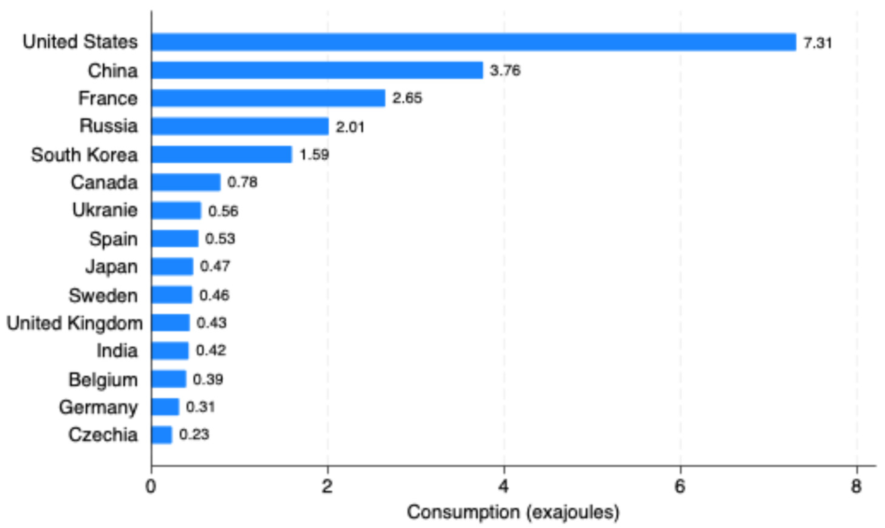
Figure 2.
The US nuclear energy production capacity and generation (2000-2022, capacity: thousand MW, generation: thousand MWh). Source: EIA.
Figure 2.
The US nuclear energy production capacity and generation (2000-2022, capacity: thousand MW, generation: thousand MWh). Source: EIA.
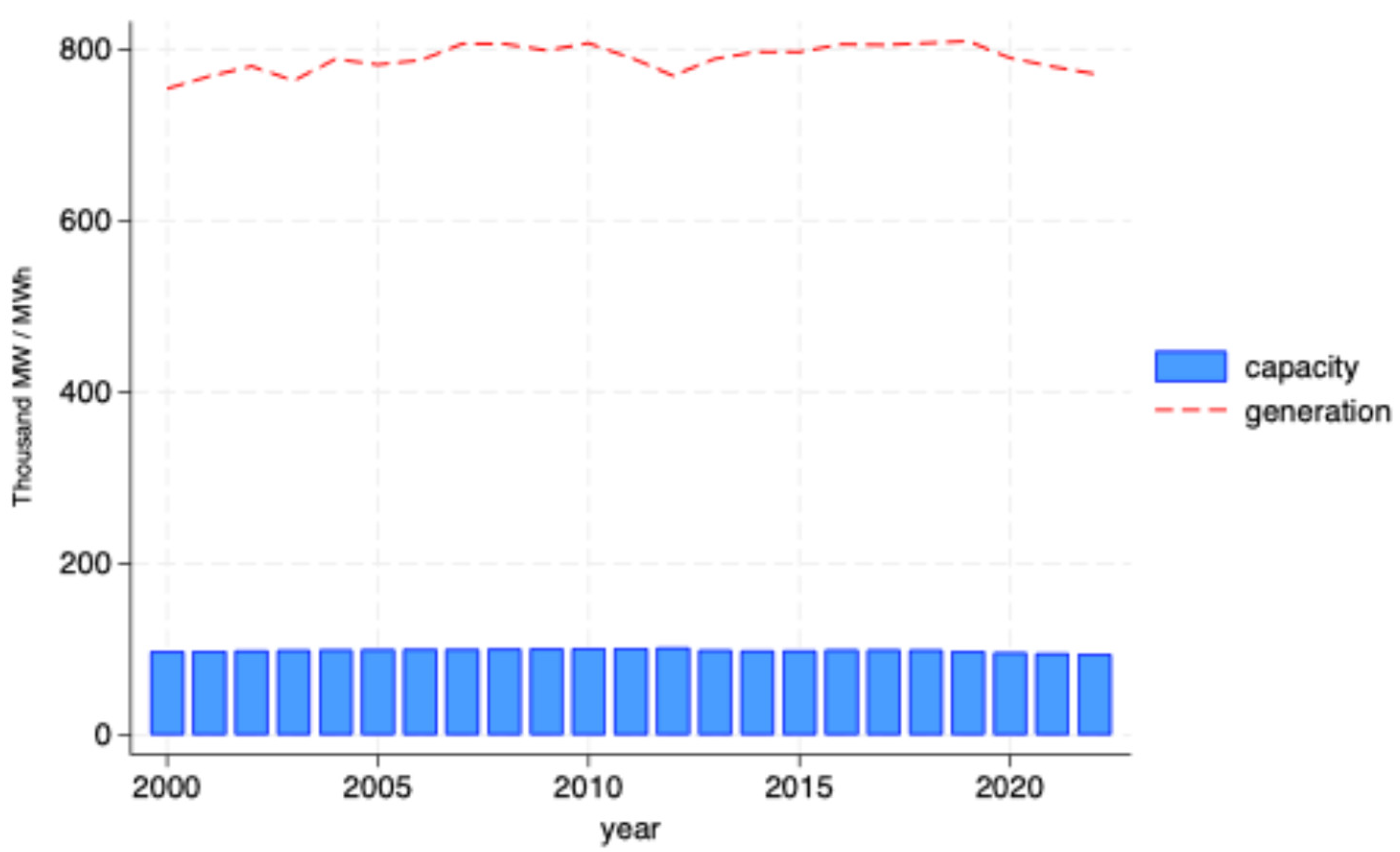
Figure 3.
Graphs of logarithmic series with structural breaks for the model (Bai-Perron test). Note: structural breaks by Bai-Perron test: 1998 and 2010.
Figure 3.
Graphs of logarithmic series with structural breaks for the model (Bai-Perron test). Note: structural breaks by Bai-Perron test: 1998 and 2010.
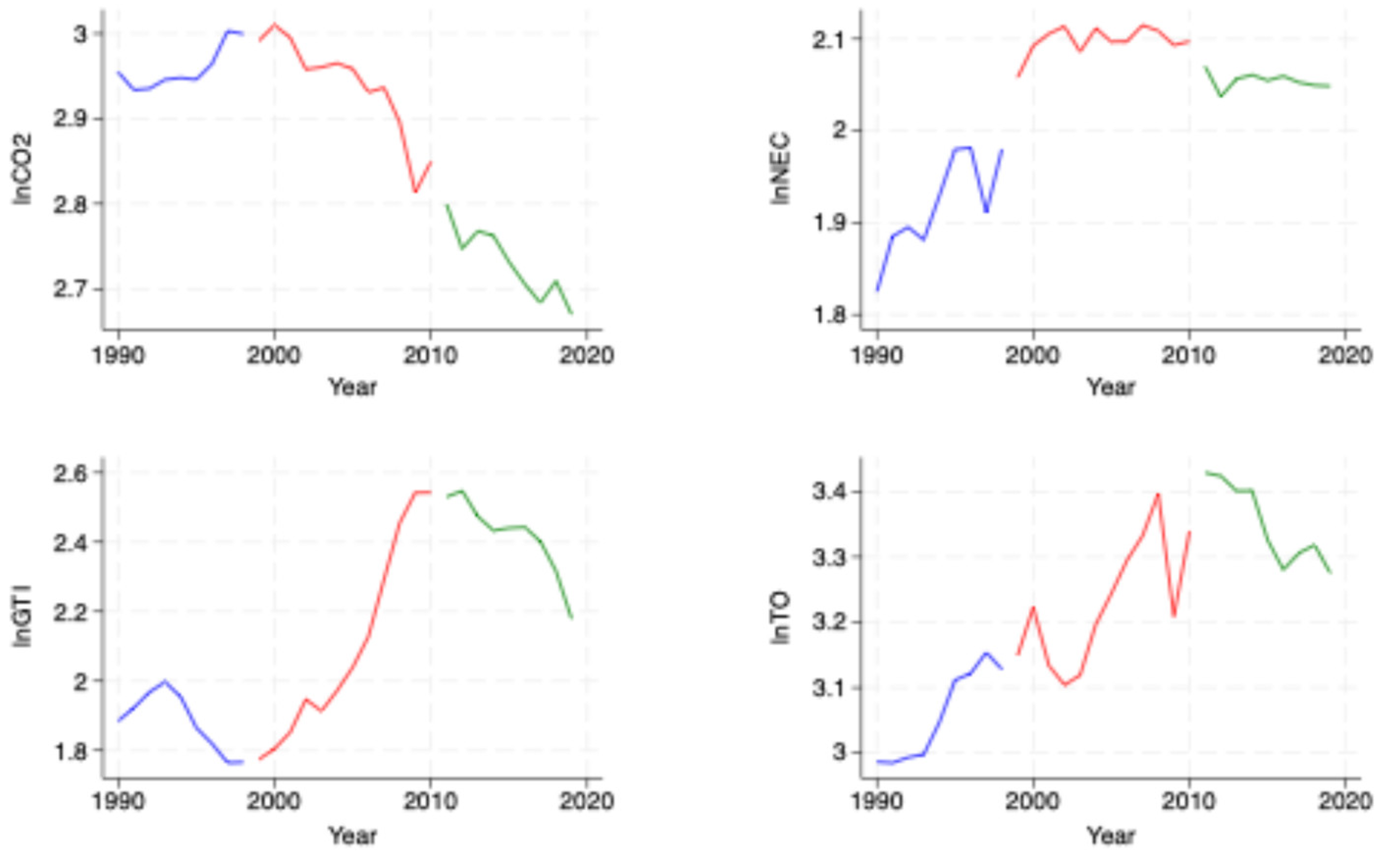
Figure 4.
CUSUM and CUSUMSQ test results.
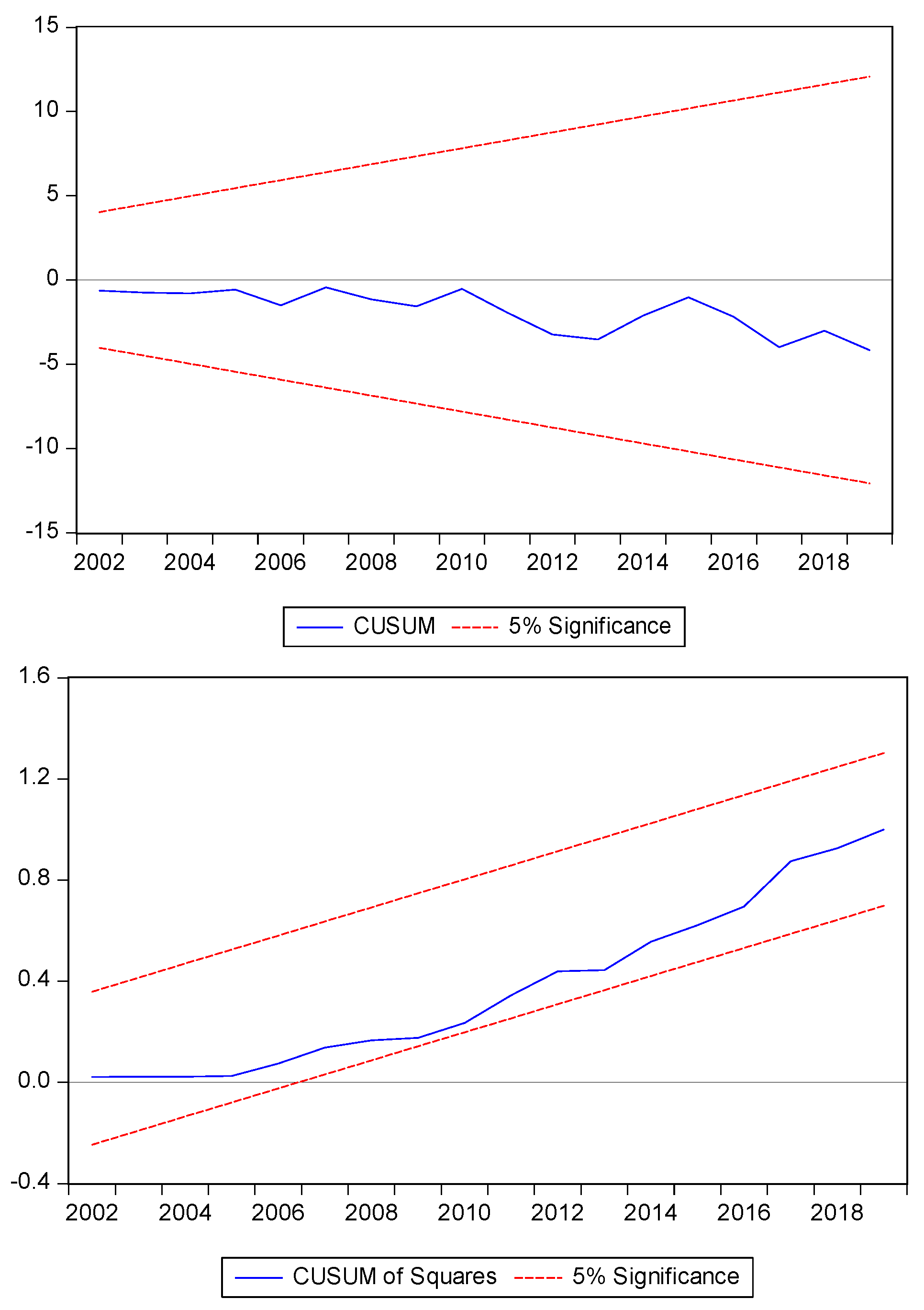

Table 1.
| Variables | Symbol | Source |
|---|---|---|
| CO2 emissions | lnCO2 | OECD Data Bank |
| Development of environment-related technologies | lnGTI | OECD Green Growth Indicators |
| Nuclear Energy Consumption | lnNEC | BP Statistical Review |
| Trade Openness | lnTO | WB-WDI |
Table 2.
Summary statistics and correlation matrix.
| lnCO2 | lnGTI | lnNEC | lnTO | |
| Mean | 2.882 | 2.132 | 2.031 | 3.214 |
| Median | 2.935 | 2.018 | 2.057 | 3.216 |
| Maximum | 3.010 | 2.547 | 2.115 | 3.428 |
| Minimum | 2.670 | 1.764 | 1.825 | 2.984 |
| Std. Dev. | 0.110 | 0.284 | 0.082 | 0.139 |
| Skewness | -0.667 | 0.230 | -1.029 | -0.118 |
| Kurtosis | 1.906 | 1.440 | 2.834 | 1.891 |
| Obs. | 30 | 30 | 30 | 30 |
| lnCO2 | 1.000 | |||
| lnGTI | -0.809 | 1.000 | ||
| lnNEC | -0.226 | 0.423 | 1.000 | |
| lnTO | -0.637 | 0.796 | 0.680 | 1.000 |
Table 3.
DF-GLS test results.
| Variables | I(0) | I(1) |
|---|---|---|
| T-statistic | T-statistic | |
| lnCO2 | 0.569 (7) | -1.803 (7)*** |
| lnGTI | -1.747 (7)*** | -1.645 (7)*** |
| lnNEC | -1.302 (7) | -3.920 (7)* |
| lnTO | -1.222 (7) | -5.811 (7)* |
Note: *, *** indicate 10% and 1% significance levels, respectively.
Table 4.
Lee Strazicich LM test results.
| Variables | I(0) | I(1) | ||
|---|---|---|---|---|
| T | Break | T | Break | |
| Results of the Test with Single Structural Break | ||||
| lnCO2 | -2.208 (3) | 2015 | -6.862 (1)* | 2000 |
| lnGTI | -4.446 (7)* | 2001 | -3.337 (4)*** | 2005 |
| lnNEC | -1.419 (6) | 2006 | -8.332 (6)* | 2011 |
| lnTO | -3.284 (3)*** | 2011 | -6.759 (0)* | 2000 |
| Results of the Test with Two Structural Breaks | ||||
| lnCO2 | -7.488 (7)* | 2006-2009 | -9.521 (8)* | 2005-2008 |
| lnGTI | -6.357 (4)** | 2005-2016 | -5.854 (5)*** | 1999-2014 |
| lnNEC | -8.049 (7)* | 2006-2009 | -15.412 (6)* | 2004-2011 |
| lnTO | -5.872 (6) | 2000-2008 | -7.860 (8)* | 2001-2011 |
Note: *, *** indicate 10% and 1% significance levels, respectively.
Table 5.
Appropriate lag length of the VAR model.
| Lag Length | LR | FPE | AIC | SIC |
|---|---|---|---|---|
| 0 | NA | 6.42e-09 | -7.512015 | -7.320039 |
| 1 | 177.5034 | 6.70e-12 | -14.39517 | -13.43529* |
| 2 | 18.16290 | 8.73e-12 | -14.21903 | -12.49125 |
| 3 | 28.88605* | 4.62e-12* | -15.09714* | -12.60145 |
Note: * indicates 10% significance level.
Table 6.
ARDL cointegration results.
| F-Bounds Test | Model |
|---|---|
| F(lnC02/lnGTI, lnNEC, lnTO) | |
| Optimal Lag Length | (3, 1, 1, 0) |
| -0.151*** | |
| F-statistics | 16.163*** |
Note: *** indicate 1% significance level.
Table 7.
ARDL long-term estimation and diagnostic test results.
| Variables | Coefficient | t | p |
|---|---|---|---|
| Constant | 5.491*** | 4.745 | 0.000 |
| lnGTI | -1.243** | -2.600 | 0.018 |
| lnNEC | -1.996* | -1.990 | 0.061 |
| lnTO | 1.233* | 1.794 | 0.089 |
| 0.988 | |||
| Adjusted | 0.983 | ||
| F-statistics | 194.238 | 0.000 | |
| Diagnostic Test Results | |||
| B-Godfrey LM Test | 1.293 | 0.271 | |
| ARCH LM Test | 1.284 | 0.306 | |
| Ramsey Reset Test | 0.283 | 0.601 | |
| J-B Normality Test | 1.271 | 0.529 |
Note: *, **, *** indicate 10%, 5% and 1% significance levels, respectively.
Table 8.
Toda-Yamamoto test results.
| Causality Direction | Chi2 | p | Decision |
|---|---|---|---|
| lnGTI→lnCO2 | 59.489 | 0.000 | GTI⇒CO2 |
| lnCO2→lnGTI | 6.786 | 0.147 | |
| lnNEC→lnCO2 | 19.397 | 0.000 | NEC⇔CO2 |
| lnCO2→lnNEC | 8.638 | 0.070 | |
| lnTO→lnCO2 | 10.631 | 0.031 | TO⇔CO2 |
| lnCO2→lnTO | 17.964 | 0.001 |
Note: ⇒ and ⇔ indicate unidirectional and bidirectional causality, respectively.
Disclaimer/Publisher’s Note: The statements, opinions and data contained in all publications are solely those of the individual author(s) and contributor(s) and not of MDPI and/or the editor(s). MDPI and/or the editor(s) disclaim responsibility for any injury to people or property resulting from any ideas, methods, instructions or products referred to in the content. |
© 2024 by the authors. Licensee MDPI, Basel, Switzerland. This article is an open access article distributed under the terms and conditions of the Creative Commons Attribution (CC BY) license (http://creativecommons.org/licenses/by/4.0/).
Copyright: This open access article is published under a Creative Commons CC BY 4.0 license, which permit the free download, distribution, and reuse, provided that the author and preprint are cited in any reuse.


