
Submitted:
15 July 2025
Posted:
16 July 2025
You are already at the latest version
Abstract
The transportation sector plays a pivotal role in economic development but is also a major contributor to environmental degradation due to its reliance on fossil fuels. This study explores the relationship between transport-related CO2 emissions, economic growth, road and rail freight transport, industry, trade openness, fossil fuel consumption, financial development, and renewable energy in 11 landlocked countries from 1990 to 2022. Using panel co-integration tests and PMG-ARDL techniques, the findings reveal a bidirectional causality between CO2 emissions, road freight, financial development, and industry. Road freight transport significantly boosts economic growth but also intensifies emissions, while renewable energy effectively mitigates transport-related CO2. The results emphasize the need for policymakers to balance economic advancement with sustainable energy and emission reduction strategies. Achieving economic-energy sustainability is essential for fostering a green and clean environment without compromising growth
Keywords:
environmental degradation
; transport-related CO2 emissions
; renewable energy consumption
; landlocked countries
; PMG-ARDL
1. Introduction
In a competitive global setting, nations utilize their natural resources to achieve higher levels of economic growth. However, they often overlook the environmental consequences of their activities, which can lead to degradation. The relationship among the transport sector, economic development, industrialization, trade openness, and in-creasing fossil fuel consumption and their combined impact on the environment has been the subject of extensive debates and academic studies in landlocked countries for quite some time. This dynamic relationship, which involves economic activity, the transport sector, and the connection between reducing fossil fuel consumption and adopting renewable energies to minimize environmental degradation, presents conflicting and paradoxical objectives for decision-makers. The transportation industry primarily relies on fossil fuels, particularly oil and gas, which release significant quantities of greenhouse gases (GHGs) and contribute to accelerating climate change (Fan et al., [1] ; Timilsina and Shrestha, [2]. The negative effects of environmental degradation are becoming increasingly evident, especially in the form of ambient air pollution. It is crucial to recognize that the power, industry, and transport sectors are the main contributors to fossil fuel-related carbon dioxide emissions globally. While there has been extensive analysis of the factors influencing CO2 emissions and emission intensities in the industry and power sectors across numerous countries, there is a notable lack of examination regarding emissions and emission intensities in the transport sector, particularly in developing nations. To ensure a sustainable future for the transport sector, it is crucial to analyze the correlation between transportation, eco-nomic growth, and the negative effects on the environment, particularly as measured by carbon dioxide emissions. Currently, research on the relationships between logistics operations, financial development, fossil fuel consumption, renewable energy consumption, and industrialization in landlocked countries is limited, especially regarding their impact on transport-related carbon dioxide emissions. Understanding how transportation contributes to environmental degradation is essential for assessing the effectiveness of current energy strategies in this sector. If required, appropriate measures should be taken to address existing issues Maryam et al.,[3]. Transportation is a vital sector for sustainability, significantly influencing the environment, economy, and society. Over the last 30 years, there has been increasing attention from policymakers, the transport industry, and academia on the concept of sustainable transportation, which is grounded in the idea of sustainable development. In this context, it is important to examine the negative impacts of transportation on sustainable development so that future policymakers can consider sustainable fuel alternatives for the transportation sector. Prioritizing the promotion of clean energy use and the re-duction of pollutant emissions is essential to fostering environmental protection. There is a strong correlation between the transportation sector's economic growth, energy consumption, CO2 emissions, and freight transport. To achieve sustainable transportation goals, it is necessary to lessen the impact of environmental change. Ensuring a clean environment for future generations presents substantial challenges for many countries worldwide. The term "landlockedness" refers to the geographical condition of a country that lacks direct access to the sea. Currently, 44 countries are classified as landlocked, with no coastal access. Among these, the United Nations identifies 32 as landlocked developing countries, which fall under the low- and middle-income categories according to the World Bank's classification. These countries face complex and interconnected economic, social, and environmental issues, necessitating the implementation of effective development policies to address these challenges Cook and Davíðsdóttir,[4] . Although the region has abundant energy supplies, its energy consumption remains a significant cause of pollution. This study significantly advances the current understanding by addressing a critical, yet underexplored, dimension of environmental economics: the specific determinants of transport-related CO2 emissions within the unique and challenging context of landlocked developing countries (LLDCs) ( Jensen,[5]; Nnene et al.,[6]) . While a considerable body of literature examines the broader nexus of economic growth, energy consumption, and emissions, there remains a conspicuous paucity of research that holistically investigates the interplay of trade openness, the distinct roles of road versus rail freight transport, financial development, industrial structure, and the pivotal contribution of renewable energy consumption in mitigating these emissions specifically for LLDCs ( Jensen, Ofélia de Queiroz et al.,[5,6,7]). Prior research has often overlooked the nuanced logistical and economic vulnerabilities inherent to these nations, or has failed to concurrently analyze this comprehensive suite of variables using robust, contemporary panel data methodologies. Consequently, this paper fills an important void by providing a focused empirical analysis of 11 LLDCs from 1990 to 2022, employing advanced panel co-integration tests and PMG-ARDL techniques. The novelty of this research lies not only in its geographical and temporal scope but also in its capacity to disentangle complex, bidirectional causal relationships and to offer granular insights into how factors such as renewable energy adoption can specifically curb transport sector emissions in these often-marginalized economies (Nnene et al.,[6] ). The findings are therefore of paramount importance for policymakers, offering a data-driven foundation for crafting targeted strategies that can promote sustainable transport, foster green economic growth, and enhance energy security, thereby guiding LLDCs towards a more resilient and environmentally sound development trajectory. The remainder of the article are arranged as follows. Section 2 reviews some background studies. Section 3 shows the proposed methodology. Section 4 presents the results. Section 5 gives a discussion on the findings and policy implications. Finally, conclusions and future researches are presented in Section 6.
2. Literature Review
Human activities, including economic activities like manufacturing goods, providing services, and utilizing infrastructure for commercial operations and transport, contribute to environmental degradation (Nathaniel,[8] ). Environmental regulations are established to safeguard individual welfare by monitoring these economic and social activities. Previous research on environmental standards has focused on evaluating the distinct relationships between transportation, industrialization, and environmental issues. These relationships are often discussed in relation to CO2 emissions. Below is an overview of the literature that highlights the connections between the variables of interest.
2.1. Nexus Between Financial Development, Energy Consumption, Economic Growth, and Environmental Degradation
The interplay among financial development, energy consumption, economic growth, and environmental degradation has been extensively researched due to its implications for sustainable development. Numerous studies highlight energy consumption, particularly from fossil fuels, as a significant contributor to environmental degradation, resulting in increased carbon dioxide (CO2) emissions and ecological harm (Raza et al.,[9]; Wada et al.,[10]). Financial development plays a critical role in this nexus, serving a dual purpose. On one hand, it facilitates investments in renewable energy and cleaner technologies, potentially mitigating environmental harm (Destek & Sarkodie,[11]; Ahmed et al., [12]). On the other hand, financial growth in certain regions, such as sub-Saharan Africa and nations involved in the Belt and Road Initiative, has been linked to increased energy consumption and ecological footprints (Baloch et al., [13]; Al-Mulali et al., [14]). Empirical studies reveal diverse causal relationships among these variables. While Gursoy-Haksevenler et al. [15] found a negative but statistically insignificant correlation between financial indicators and energy consumption. Similarly, Vidyarthi [16] observed a reciprocal long-term relationship between GDP and energy consumption in South Asia, along with a unidirectional relationship where CO2 emissions influence both GDP and energy consumption. In OECD nations, the EKC hypothesis has been validated, with CO2 emissions declining after reaching a certain stage of economic development (Hassan and Salim, [17] ). Notably, findings by Ahmed et al. [18] using a Vector Error Correction Model (VECM) suggest that energy consumption, GDP, and CO2 emissions are co-integrated in the long term, underscoring the enduring interdependence of these variables. Collectively, this body of research emphasizes that aligning financial development and economic growth with sustainable energy practices and robust environmental policies is essential for effectively mitigating environmental degradation.
2.2. Nexus Between Renewable Energy, energy consumption and environmental degradation
The global transition to clean energy, aimed at reducing CO2 emissions, combating climate change, and promoting renewable energy (RE), has been extensively studied Mohammed et al.,[19]. In the EU, Bölük and Mert [20] reported that both RE and NREC increased CO2 emissions, whereas Jebli and Ozturk [21] observed reductions in CO2 emissions in 25 OECD countries due to RE. Similarly, Bilgili et al. [22] found that RE significantly decreased emissions in 17 OECD countries (1977–2010), Zoundi [23] and Hu [24] confirmed the positive impact of RE on emissions reduction in sub-Saharan Africa and 25 developing countries, respectively. Sharif et al. [25] , using data from 74 countries, highlighted that energy consumption (EC) increases emissions while RE reduces them. In the transportation sector, Raihan et al. [26] and Wang et al. [27] emphasized the benefits of RE, including enhanced energy security and reduced dependence on fossil fuels. Specific studies, such as those by Murshed and Elheddad [28] in Argentina and Zahoor et al. [29] in China, con-firmed that RE effectively lowers emissions in this sector. Finally, the relationship be-tween RE and economic growth (GDP) has been explored, with Fan and Hao [30] identifying a stable, unidirectional effect of GDP on RE in 31 Chinese provinces (2000–2015).
2.3. Nexus Between Trade Openness and Environmental Degradation
The relationship between trade openness and environmental quality, particularly carbon dioxide (CO2) emissions, has been a focal point in economic and environmental research. For instance, Gu et al.[31] identified a unidirectional causal relationship, where foreign trade dependency influences CO2 emissions. Contrarily, Akin [32] argued that trade openness decreases CO2 emissions, establishing a unidirectional link from CO2 to trade openness. Several studies have examined the regional impacts of trade openness. Hakimi and Hamdi [33] attributed negative environmental impacts in Morocco and Tunisia to trade openness. Similarly, Ling et al. [34] reported a positive correlation between trade openness and CO2 emissions in the ASEAN-5 countries (Indonesia, Malaysia, the Philippines, Singapore, and Thailand) from 1995 to 2014, indicating a bidirectional relationship. Boutabba [35] , in an analysis of India, found a negative association between trade openness and CO2 emissions, highlighting a long-term equilibrium.
In Sri Lanka, Naranpanawa [36] concluded that while there is no long-term causality between trade openness and CO2 emissions, short-term connections are evident. Meanwhile, Ertugrul et al. [37], focusing on ten developing countries (e.g., China, India, Brazil, and South Africa) from 1971 to 2011, identified co-integration among trade openness, energy consumption, real income, and CO2 emissions, supporting the EKC hypothesis in several nations. In the United States, Dogan and Turkekul [38] demonstrated a reciprocal relationship between CO2 emissions and trade openness from 1960 to 2010, emphasizing the importance of trade openness and urbanization in managing GDP and pollution. Zamil et al. [39] observed a positive relationship between trade openness, GDP per capita, and CO2 emissions in Oman, urging policymakers to integrate environmental considerations into trade policies. Rahman et al. [40] explored South Asia (1990–2017), finding a negative relationship between trade openness, CO2 emissions, and economic growth, alongside unidirectional causality between these variables. Similarly, Yu et al. [41], studying Commonwealth of Independent States (CIS) countries (2000–2013), found a direct positive impact of trade openness on CO2 emissions but a negative indirect effect via reduced per capita income. Lastly, Jun et al. [42], through wavelet-coherence analysis, demonstrated a dynamic relationship between trade openness and CO2 emissions in China. Their findings highlighted the necessity for China to adopt strategies to mitigate pollution while pursuing trade liberalization.
2.4. Nexus Between Freight Transportation and Environmental Degradation
The relationship between transportation, energy consumption, economic growth, and environmental degradation has been a significant area of research, with findings highlighting various regional and sectoral dynamics. Adoms et al. [43] examined the long-term correlation between road transport energy consumption and economic growth in six West African countries, identifying a unidirectional causal relationship from income to transport energy consumption using the Dumitrescu-Hurlin panel causality test. In Tunisia, Achour and Belloumi [44] revealed a positive link between GDP, transport value-added, infrastructure, and CO2 emissions from 1971 to 2012, though no reverse causality was observed. Neves et al. [45] , focusing on 15 OECD countries from 1995 to 2014, found that rail infrastructure investment could reduce fossil fuel usage and CO2 emissions, highlighting the potential of sustainable transport policies. Further studies emphasized the environmental impact of freight transport. Song et al. [46] reported a 13,49 % annual increase in traffic-related energy consumption in Shanghai from 2000 to 2010, while Murtishaw and Schipper [47] identified growing reliance on trucks in the U.S. as a driver of higher energy intensity. Linton et al. [48] forecast a 72% increase in rail transport energy use by 2050, with corresponding CO2 emissions. Saidi and Hammami [49] emphasized the transportation sector's role in global carbon emissions, while Shafique et al. [50] advocated for sustainable policies and technological advancements to mitigate these impacts. Collectively, these studies underscore the urgent need for environmentally conscious transportation strategies to balance economic growth with sustainability.
2.5. Nexus Between Industrialization and Environmental Degradation
The relationship between industrialization, energy consumption, economic growth, and environmental degradation has been extensively studied, with research consistently highlighting the role of industrialization in increasing carbon emissions. Carvalho et al. [51] emphasized that industrialization often prioritizes economic development at the expense of environmental sustainability. However, few studies have simultaneously examined the combined impact of industrialization, energy consumption, economic growth, and financial development on environmental degradation. Empirical evidence supports a positive link between industrialization and CO2 emissions in various regions. For instance, Wang and Liu [52] identified this association in Western developing countries, while Abu-Ali et al. [53] confirmed it for Arab regions. Rafiq et al. [54], using the STIRPAT model, demonstrated a positive relationship between industrialization and CO2 emissions across 53 countries. Similar findings were reported by Nejat et al.[55] and Tian et al.[56] in China, Salim and Shafiei [57] in OECD countries, and Cherniwchan [58] across 157 countries. Shahbaz et al. [59] also established a link between industrialization and CO2 emissions in Bangladesh. Several studies have explored the dynamics between industrialization, energy consumption, and environmental degradation. Asumadu-Sarkodie and Owusu [60] found a long-term relationship between carbon emissions, energy use, industrialization, and financial development in Sri Lanka (1971–2012), identifying a unidirectional causal relationship from energy consumption to carbon emissions and a bidirectional relationship between industrialization and energy use. Similarly, Asumadu-Sarkodie and Owusu [61] revealed a significant long-term link between industrialization and CO2 emissions in Rwanda (1965–2011), highlighting detrimental effects on health and air quality, and recommending environmentally friendly industrial policies. Appiah et al.[62] and Anwar and Elfaki [63] highlighted industrialization's importance in promoting innovation and resource allocation but noted its environmental costs, particularly through increased energy consumption and CO2 emissions. Nasrollahi et al.[64] underscored the positive impact of industrialization on economic growth, despite its challenges. As industrialization drives energy demand, its environmental implications become evident, necessitating policies that balance economic growth with environmental sustainability through technological advancements and structural reforms.
3. Data and Methodology
3.1. Data
Based on the availability of data, we use a panel of 11 landlocked Countries between 1990 to 2022 using the World Development Indicator (WDI) and the International Energy Agency (IEA 2024) [65] dataset. This particular period was chosen simply because the required data was not available for earlier periods. The selected landlocked countries included in the sample are Armenia, Austria, Azerbaijan, Belarus, Hungry, Kazakhstan, Luxembourg, Slovakia, Switzerland, and Uzbekistan. The inclusion of these nations is motivated by the distinctive challenges faced by landlocked countries, such as reliance on transit nations for access to international markets, inadequate transportation infrastructure, complex customs and border procedures, and limited access to maritime trade routes, all of which significantly influence their economic and environmental dynamics. In this analysis, transport-related carbon dioxide emissions (TCO2) were considered a dependent variable, and the factors of road freight transports (ROFT), rail freight transport (RAFT), gross domestic product (GDP), industry value added (IND), Fossil fuel energy consumption (EC), trade openness (TOP), renewable energy consumption (RE), and financial development (FD) were examined as explanatory variables. To ensure that the data is normally distributed, the parameters were converted into logarithmic forms. Details about the variables used in this study along with the measurement and source of data are given in Table 1.
3.2. Empirical Model
Using Transport based CO2 emission (TCO2) as our dependent variable modelled as a function of road freight transports (ROFT), rail freight transport (RAFT), gross domestic product (GDP), industry (IND), Fossil fuel energy consumption (EC), trade openness (TOP) , renewable energy consumption (RE) and financial development (FD): manuscripts reporting large datasets that are deposited in a publicly available database should specify where the data have been deposited and provide the relevant accession numbers. If the accession numbers have not yet been obtained at the time of submission, please state that they will be provided during review. They must be provided prior to publication.
The econometric model specification is provided as follows in Equations 1 :
Where,, represent the elasticities of the variables in the model with respect to TCO2. represents time and is the error term. The log form safeguards the removal of likely outliers as well as large coefficients. Elasticities are of importance as they bring to bear the actual responses of TCO2 as the dependent variable, against road freight transports (ROFT), rail freight transport (RAFT) gross domestic product (GDP) industry (IND), Fossil fuel energy consumption (EC), trade openness (TOP), renewable energy consumption (RE) and financial development (FD). indicates the country index and is period of 1990 to 2020, and indicating the constant and the classical error term respectively. represents the estimated coefficients of all independent variables where
3.3. The Flowchart of the Analysis
This study implements a comprehensive panel econometric methodology to examine the long- and short-run dynamics between transport-related CO₂ emissions and a set of macroeconomic and energy-related variables. First, cross-sectional dependence (CSD) is assessed using the Breusch-Pagan LM test, Pesaran’s scaled LM, bias-corrected scaled LM, and the CD test, which evaluate the interdependence of panel units by analyzing residual correlations. To address parameter heterogeneity, Pesaran et al.’[66] slope homogeneity test—comprising the delta (Δ̃) and adjusted delta (Δ̃_adj) statistics—is employed to determine whether cointegration slopes are consistent across units. Second-generation panel unit root tests, namely the Cross-Sectional Augmented Dickey-Fuller (CADF) and the Cross-Sectionally Augmented IPS (CIPS) tests, are used to account for cross-sectional dependencies while testing the stationarity of individual series. Panel cointegration is examined using the Pedroni and Kao residual-based tests. Pedroni’s test allows for heterogeneity in both intercepts and slopes, using seven statistics across within- and between-dimension estimators, while the Kao test assumes homogeneity in cointegration relationships but includes individual fixed effects. The long- and short-run relationships are further estimated using the Pooled Mean Group Autoregressive Distributed Lag (PMG-ARDL) model, which captures the dynamic adjustment of TCO₂ emissions to its equilibrium path. For robustness, Fully Modified OLS (FMOLS) and Dynamic OLS (DOLS) estimators are employed to control for endogeneity and serial correlation in the long-run estimations. Finally, causality is explored using the Dumitrescu and Hurlin (DH) panel causality test, which is suitable for heterogeneous panels with cross-sectional dependence. This approach leverages the average (W̄) and standardized (Z̄) statistics to test for Granger-type causality between variables, guiding the formulation of targeted environmental and transport policies based on the directionality of influence among variables. Additionally, the Impulse Response Function (IRF) is utilized to trace the dynamic response of TCO₂ emissions to one-time shocks in explanatory variables, offering insights into the magnitude and persistence of the effects over time. Complementarily, Variance Decomposition Analysis (VDA) quantifies the relative contribution of each explanatory variable to the forecast error variance of TCO₂ emissions, thereby identifying the dominant sources of variation and policy leverage points. This integrated methodological approach ensures robust inference for guiding environmental and transport-related policy formulation in heterogeneous panel settings. The Figure 1 presents the flow chart methodology followed up in the empirical examination.
3.4. Cross-Sectional Dependence Test
The empirical study is beginning by the CSD test of full sample and subsample (Europe and Asia) by employing the Breusch and Pagan LM test, the Pesaran scaled LM test, the Bias-corrected scaled LM test and the Pesaran CD test. Pesaran’s Cross-Sectional Dependence (CD) test is predicated on the mean pairwise correlation of residuals and is presented as follows:
Where is the pairwise correlation coefficient of residuals between units i and j, N represents the number of cross-sectional units, T represents the number of time periods. The null hypothesis should be accepted when there is CSD in the panel data.
3.5. Slope Homogeneity Test
A slope homogeneity test for panel data models attributed to Swamy [68] developed the framework to find if slope coefficients of the cointegration equation are homogenous. Pesaran and al [66] improved Swamy’s slope homogeneity test formed two ‘delta’ test statistics; and .
Where is the number of cross-section unit is, denotes the Swamy test statistic, is the independent variables, and are suitable for large and small samples, respectively. The null and alternative hypothesis used for slope homogeneity test is as follows:
: Cointegration coefficients are homogenous.
: Cointegration coefficients are heterogeneous.
3.6. Panel Unit Root Test
In this study, two second-generation panel root tests, specifcally the Cross-Sectional Augmented Dickey-Fuller (CADF) and Augmented Cross-Sectional Im, Pesaran, and Shin (CIPS) test Pesaran,[67] were employed. The CADF model can be presented as follows in Eq. (6):
Where =
The CIPS statistic is the mean value of t-statistics that are obtained from estimating the CADF regression for each cross section:
Where the CADFi is the cross-sectional augmented Dickey-Fuller statistics for ith cross-section unit and N represents a cross-sectional dimension. In the context of unit root test, the null hypothesis postulates that all series within the panel follow a non-stationary process, whereas the alternative hypothesis proposes that a fraction of the series in the panel is characterized by stationarity.
3.7. Panel Cointegration Test
This study adopts two panel cointegration tests, namely the Pedroni residual cointegration test Pedroni, [69] and the Kao test ,[70]. Pedroni [69] introduces statistics that examine the hypothesis of no cointegration in nonstationary panels. These statistics account for both within-dimension (panel statistics) and between-dimension (group statistics) variations, allowing for heterogeneity in the short-run dynamics, as well as in the long-run intercepts and slope coefficients across cross-sectional units. This flexibility makes the Pedroni test particularly suitable for heterogeneous panel structures commonly encountered in macroeconomic and environmental studies.
The entire test statistics are residual-based tests, with residuals collected from the following regressions:
Where is the number of individuals in the panel, is the number of time periods, is the number of regressors, and is the number of lags in the ADF regression.
Kao [70] proposes estimating the homogeneous cointegrating relationship through pooled regression, while accounting for individual fixed effects. The regression equation is as follows:
The least squared dummy variable (LSDV) estimator for is:
Where and . The residuals from this first stage regression will still contain a unit root under the null hypothesis of no cointegration.
3.8. Pooled Mean Group (PMG-ARDL) Results
The model specification of panel linear ARDL model (p, q) developed by Pesaran et al. (1999) is given in Eq (14):
Where TCO2 is the dependent variables and indicates the transport carbon dioxide emission is (k vector of explanatory variables including of road freight transports, rail freight transport, gross domestic product, industry, Fossil fuel energy consumption, trade openness and renewable energy consumption. represents the fixed effects , is the coefficient of the lagged dependent variable , is (k coefficient vector of independent variables ,is the error term , i(1,2,..N) is the number of cross section , and t (1,2,…T) denotes the time . The absence of long run relationship among the variables is represented as null hypothesis. By transforming eq. (15), we obtain the panel ARDL (p, q) error correction model:
Where , and provide both short-run dynamics and the long run information contained in the data respectively. Additionally, denotes the error correction term to evaluate the speed of adjustment of TCO2 emissions toward its long run equilibrium with the variation in explanatory variables.
3.9. Robustness Check
The Fully modifed ordinary least square (FMOLS) showed the ability to tackle endogeneity and serial correlation in long-run relationships. Following Pedroni, [71] , the panel FMOLS estimator is expressed as:
Where is the FMOLS estimator applied to each country and the associated t-statistic is:
The Dynamic Ordinary Least Square (DOLS) is a parametric model recommended by McCoskey and Kao[70] and Mark and Sul [72] for the first time. DOLS is appropriate for small samples compared to OLS and FMOLS and is used for the long-run analysis to take into account the potential heterogeneity and serial correlation. Following Alvarez and al.[73], the DOLS method is expressed as:
Where asymptotically eliminates the endogeneity of on the distribution of the OLS estimator of β, shows maximum lag length, shows maximum lead length, and shows a Gaussian vector error process.
3.10. Dumitrescu Hurlin (DH) Panel Causality Tests
The DH test is based on an average of individual Wald statistics from N cross-sectional regressions:
where is the Wald statistic for unit i.
The standardized statistic is given by:
After analyzing the long and short-run relationship, it is crucial to analyze the causal relationship to guide better policies. To ascertain the association between the dependent variable represented by carbon dioxide emission from transportation and the independent variables in landlocked countries, we employ the panel causality test developed Dumitrescu and Hurlin [74] . The advantage of Dumitrescu Hurlin (DH) panel causality test is their ability to analyzing data in the presence of sectional dependence between countries. The DH panel causality test use two different statistics: the Wbar statistics and the Zbar statistics. The Wbar statistics take an average of test statistics, while the Zbar statistics designate a standard normal distribution. If the p-value is less than 5%, 10% and 1% the causality test rejects the null hypothesis.
4. Empirical Results and Discussion
4.1. Descriptive Analysis
Table 2 provides a comparative analysis of descriptive data for all sample, european and Asian LLc. A general overview of the descriptive statistics reveal notable regional differences across the variables. On average, European LLc report higher total carbon emissions (lnTCO2 = 3.158) and GDP levels (lnGDP = 9.599) than their Asian counterparts (lnTCO2 = 2.333; lnGDP = 7.499), reflecting greater economic maturity and associated environmental externalities. Renewable energy use in European LLC is significantly higher (mean = 11.929) compared to Asian LLC (mean = 0.938), indicating a stronger commitment to green energy transition. Standard deviation values reveal substantial variability in industrial activity, particularly in European LLC (Std. Dev. = 7.472) and the full sample (Std. Dev. = 6.333), suggesting a wide range of industrialization levels across countries.
4.2. Cross Sectional Dependence Test
As shown in Table 3, all statistical tests are significant at the 1% level, which leads to the rejection of the null hypothesis of no cross-sectional dependence and acceptance of the alternative hypothesis of cross-sectional dependence at the 1% significance level in the panel variables. These findings imply that the variables of landlocked countries are cross-sectionals dependent; suggesting that shocks occurring in one of the 11 landlocked countries seems to be transmitted to other countries. In order to tackle this significant matter, the null hypothesis of the test posits that CSD is not present in the data.

Table 3.
Results of cross-sectional dependence analysis test for all sample, European and Asian-LLc.
Table 3.
Results of cross-sectional dependence analysis test for all sample, European and Asian-LLc.
| Breusch-Pagan LM | Pesaran scaled LM | Bias-corrected scaled LM | Pesaran CD | |
| All sample-LLc | ||||
| lnTCO2 | 776.236 (0.000) *** | 68.767 (0.000) *** | 68.595 (0.000) *** | 21.246 (0.000) *** |
| lnROFT | 735.059 (0.000) *** | 64.841 (0.000) *** | 64.669 (0.000) *** | 24.921 (0.000) *** |
| lnRAFT | 435.153 (0.000) *** | 36.246 (0.000) *** | 36.074 (0.000) *** | 6.876 (0.000) *** |
| lnFD | 370.518 (0.000) *** | 30.083 (0.000) *** | 29.911 (0.000) *** | 11.440 (0.000) *** |
| lnGDP | 1542.792 (0.000) *** | 141.855 (0.000) *** | 141.683 (0.000) *** | 39.187 (0.000) *** |
| lnIND | 1085.402 (0.000) *** | 98.244 (0.000) *** | 98.073 (0.000) *** | 31.677 (0.000) *** |
| lnEC | 650.825 (0.000) *** | 56.809 (0.000) *** | 56.637 (0.000) *** | 10.302 (0.000) *** |
| lnTOP | 917.698 (0.000) *** | 82.255 (0.000) *** | 82.083 (0.000) *** | 28.152 (0.000) *** |
| lnRE | 461.787 (0.000) *** | 38.785 (0.000) *** | 38.613 (0.000) *** | 15.105 (0.000) *** |
| European-LLc | ||||
| lnTCO2 | 476.746 (0.000) *** | 70.323 (0.000) *** | 70.213 (0.000) *** | 21.753 (0.000) *** |
| lnROFT | 269.915 (0.000) *** | 38.408 (0.000) *** | 38.299 (0.000) *** | 14.507 (0.000) *** |
| lnRAFT | 197.594 (0.000) *** | 27.249 (0.000) *** | 27.139 (0.000) *** | 2.525 (0.011) ** |
| lnFD | 102.947 (0.000) *** | 12.644 (0.000) *** | 12.535 (0.000) *** | 4.072 (0.000) *** |
| lnGDP | 629.852 (0.000) *** | 93.947 (0.000) *** | 93.838 (0.000) *** | 25.081 (0.000) *** |
| lnIND | 387.646 (0.000) *** | 56.574 (0.000) *** | 56.465 (0.000) *** | 18.605 (0.000) *** |
| lnEC | 293.971 (0.000) *** | 42.120 (0.000) *** | 42.011 (0.000) *** | 15.467 (0.000) *** |
| lnTOP | 343.282 (0.000) *** | 49.729 (0.000) *** | 49.619 (0.000) *** | 16.981 (0.000) *** |
| lnRE | 412.020 (0.000) *** | 60.335 (0.000) *** | 60.226 (0.000) *** | 19.988 (0.000) *** |
| Asian-LLc | ||||
| lnTCO2 | 34.127 (0.000) *** | 8.119 (0.000) *** | 8.057 (0.000) *** | 0.645 (0.518) |
| lnROFT | 69.731 (0.000) *** | 18.397 (0.000) *** | 18.335 (0.000) *** | 7.984 (0.000) *** |
| lnRAFT | 26.741 (0.000) *** | 5.987 (0.000) *** | 5.925 (0.000) *** | 1.517 (0.129) |
| lnFD | 49.639 (0.000) *** | 12.597 (0.000) *** | 12.535 (0.000) *** | 6.676 (0.000) *** |
| lnGDP | 160.542 (0.000) *** | 44.612 (0.000) *** | 44.550 (0.000) *** | 12.643 (0.000) *** |
| lnIND | 147.389 (0.000) *** | 40.815 (0.000) *** | 40.753 (0.000) *** | 12.117 (0.000) *** |
| lnEC | 49.186 (0.000) *** | 12.466 (0.000) *** | 12.404 (0.000) *** | -1.154(0.248) |
| lnTOP | 116.111 (0.000) *** | 31.786 (0.000) *** | 31.723 (0.000) *** | 10.600 (0.000) *** |
| lnRE | 24.201 (0.000) *** | 5.254 (0.000) *** | 5.191 (0.000) *** | -1.097(0.272) |
Source: Author own calculation by using E-Views 12 Notes: Null hypothesis: No cross-section dependence (correlation), *** and ** indicate rejection of the null hypothesis at 1% levels of significance; numbers in parentheses are P-values.
4.3. Slope Homogeneity Test
Table 4 reported the results of Pesaran and Yamagata [75] slope homogeneity test. It is shown that the null hypothesis is significant at 1% level: confirming the homogenous data. The delta test results confirm that slope coefficients are heterogeneous in the CSD, and the model of the analysis has the heterogeneity problem. The results of these tests confirm the CSD and slope heterogeneity in the sample of landlocked countries. We consider the second-generation panel unit-root tests more appropriate for our analysis.
by subheadings. It should provide a concise and precise description of the experimental results, their interpretation, as well as the experimental conclusions that can be drawn.
4.4. Panel Unit Root Test
The Table 5 displays the results of the unit root test in both the level and first difference. The results of the second-generation panel unit root tests (CIPS and CADF) reveal a mixed order of integration across the variables. According to the CIPS test, in the full sample, all variables are non-stationary at level except for GDP and TCO2, a pattern mirrored in the European subsample. In Asia, however, EC, RE, and TCO2 are stationary at level. The CADF test shows that for the full sample, all variables are non-stationary at level except for GDP and IND, while in Europe, only TCO2 is stationary. In Asia, RAFT, FD, and RE are stationary at level. These findings indicate that some variables are integrated of order I(0), while others are I(1), confirming a combination of different integration levels. The consistency between the CIPS and CADF tests supports the suitability of the PMG-ARDL approach, which can handle variables with mixed integration orders, for robust and reliable analysis.
4.5. Panel Cointegration Test
The Table 6 reported the panel cointegration tests results. The Pedroni cointegration test results reveal that the panel PP-Statistic and the panel ADF-Statistic exhibit significant findings at a 1% level of significance. As a result, we can conclude that there is evidence of cointegration between the variables. Furthermore, the ADF statistic of the Kao test is found to be significant at a 1% significance level. Thus, the study confirms the stable relationship between the variables in the long run and eliminates the possibility of deceiving regression in the model. The findings of this study suggest that any disruption to sustainable transportation will have a lasting impact on carbon dioxide emissions. Therefore, it is crucial to assess the long-term and short-term impacts by utilizing the PMG estimator within the framework of the ARDL model. This section may be divided by subheadings. It should provide a concise and precise description of the experimental results, their interpretation, as well as the experimental conclusions that can be drawn.
4.6. PMG-ARDL Results
As reported in Table 7, the results of the PMG-ARDL estimation provide valuable insights into the determinants of transport-related CO2 emissions (TCO2) across the full sample, Europe, and Asia, highlighting both long-run and short-run dynamics. For the full sample, financial development (FD) and gross domestic product (GDP) exhibit a positive and significant long-run relationship with TCO2, suggesting that economic growth and financial expansion contribute to increased emissions. Conversely, rail freight transport (RAFT), industry (IND), energy consumption (EC), and trade openness (TOP) demonstrate a negative and significant impact on TCO2, indicating their potential role in mitigating emissions. Notably, road freight transport (ROFT) and renewable energy (RE) show a positive but insignificant relationship with TCO2, diverging from prior studies such as Zhen et al. [76] . In the short run, the error correction term is negative and significant, confirming the model's convergence to equilibrium, while trade openness (TOP) is the only variable with a significant positive impact on TCO2. For Europe, the long-run results reveal that ROFT, IND, and RE significantly increase TCO2, while FD, GDP, and TOP have a significant negative effect, underscoring the region's unique economic and industrial dynamics. In Asia, all variables except TOP are significant in the long run, with ROFT, FD, GDP, RE, and EC increasing TCO2, while RAFT and IND reduce emissions. This suggests that rail freight and industrial activities in Asia play a crucial role in lowering emissions, potentially due to efficiency gains or cleaner technologies. The short-run analysis for Asia highlights GDP as the only significant variable, with a negative impact on TCO2, reflecting the region's transitional economic adjustments. Across all samples,
The negative and significant error correction terms indicate that the TCO2 models converge to their long-run equilibrium, reinforcing the robustness of the findings. These results align with prior literature, such as Hasanov et al. [77] , while also offering region-specific insights. Policymakers should consider these findings to design targeted strategies, such as promoting rail freight transport and renewable energy in Asia, enhancing industrial efficiency in Europe, and balancing economic growth with environmental sustainability globally. The graphical representation in Figure 2 further illustrates the regional variations in the long-run determinants of TCO2, emphasizing the need for tailored policy interventions to address the diverse challenges of transport-related emissions.
4.7. Robustness Check
Table 8 reports the estimation results of FMOLS for full, European and Asian LLc, which are in line with the baseline estimations. In table 6, As one would expect, using each of the three samples, we find that the effect of indicators for sustainable transportation on carbon dioxide emission from landlocked countries is larger and statistically significant at the 1% level, except for Road freight transports in Europe landlocked countries which have a positive impact but not significant. Similar to FMOLS estimations, Results from DOLS show the influence of the variables employed in the study on carbon dioxide emission from transport in landlocked countries. Except of EC and TOP in entire sample, ROFT in Europe sample and RE in Asian sample, all other indicators have highly significant impact on TCO2. Overall, our robustness analysis confirms that indicators for sustainable transportation have a strong effect on carbon dioxide emission from landlocked countries for both entire sample and subsamples in the long-run. While the effect of variable under consideration is highly significant in the long-run for different estimates (ARDL, FMOLS and DOLS), their effect is weakly significant in short run. Additionally, in short-run, entire sample, Europe and Asia respond to different extents. Finally, none of the estimated coefficients is significant for the case of Europe in short-run.
4.8. Dumitrescu Hurlin (DH) Panel Causality Tests
The results of DH test are reported in Table 9 and figure 2. The DH test, developed by Dumitrescu and Hurlin [74], constitutes a robust extension of the traditional Granger causality test adapted for heterogeneous panel data. This methodology offers the significant advantage of allowing coefficient variation across cross-sectional units (countries) while maintaining the assumption of temporal stationarity (Lopez and Weber, [78]).In the full sample-LLc, bidirectional causality is observed between TCO₂ and RAFT, FD, GDP, IND, and RE, supporting the findings of Khan et al. [79], who also identified similar bidirectional links. A unique unidirectional causality from TCO₂ to ROFT suggests that changes in emissions influence road freight activity, echoing McKinnon’s [80] conclusions about the regulatory impact of decarbonization efforts. Additionally, EC is found to unidirectionally cause TCO₂, consistent with the IEA’s (2021) [81] observations on fossil fuel dependency in transport. In European-LLc, the causal relationships are more interconnected. TCO₂ has bidirectional causality with all key variables (ROFT, RAFT, FD, GDP, IND, RE), reflecting deeper integration of environmental and economic policies across the EU (EEA, 2019 [82]). Interestingly, TCO₂ also unidirectionally causes EC, indicating that emission variations influence fossil energy use, likely due to carbon reduction policies that drive cleaner technologies (Arbolino et al., [83]). Another unique finding in European-LLc is the unidirectional causality from TCO₂ to TOP, implying that emission concerns may shape trade behaviors through mechanisms like carbon tariffs or consumer demand for low-emission goods.
4.9. Dynamic Impact Analysis
Figure 3 to figure 5 displays the impulse response analysis (IRF) conducted for the full sample, European, and Asian-LLc. Across all samples, a positive response of ROFT to TCO₂ shocks underscores the strong linkage between freight intensity and emissions, although the effect stabilizes over time, especially in Europe, suggesting greater long-term regulation or infrastructure efficiency (Ćosović et al., [84]). This aligns with findings from Saha et al. [85], who underscore the environmental inefficiency of road-centric freight systems in Bangladesh and advocate for modal shifts. Conversely, RAFT reacts differently across regions: while the full sample shows a modest short-term increase, European countries exhibit a positive but muted response, whereas Asian countries demonstrate a negative and declining trend, indicating that rail serves as a more climate-friendly alternative in Asia. GDP initially declines in response to TCO₂ shocks in the full sample, suggesting emission-related economic costs. This effect is more pronounced in Europe, where environmental regulations may act more stringently, while in Asia the effect is slightly weaker (Rabbi and Abdullah, [86]). Industrial output (lnIND) generally rises with emissions, more strongly in Asia, reflecting a carbon-intensive industrial structure, whereas Europe's weaker response may be due to higher energy efficiency or cleaner production technologies (Holappa, [87]). Fossil fuel consumption (lnEC) displays a robust and consistent positive response in all samples, confirming transport's dependence on fossil energy (Lei et al., [88]). However, renewable energy consumption (lnRE) responds negatively or insignificantly, especially in Asia, suggesting a sluggish green energy transition; only Europe shows a sustained negative response, hinting at stronger renewable integration mechanisms (Vo et al., [89]). This is supported by Hariyani et al.[90], who found trade openness and financial development also influence emissions dynamics in East Asia-Pacific economies. Trade openness (lnTOP) is marginally affected by TCO₂ shocks: mildly negative in Europe and slightly positive in Asia, indicating that emissions may dampen trade more where environmental policies are stricter. Financial development (lnFD) initially contracts following emissions shocks in all samples, especially in Asia, but gradually rebounds, suggesting that financial systems adapt over time to environmental externalities (Nasrullah et al.,[91]). These findings point to the persistent carbon dependency of freight systems and economic structures in landlocked countries, while also revealing regional asymmetries in green transition trajectories. For policy, a modal shift from road to rail, enhanced renewable integration, support for green finance, and industrial decarbonization remain central to reconciling logistical efficiency with environmental sustainability.
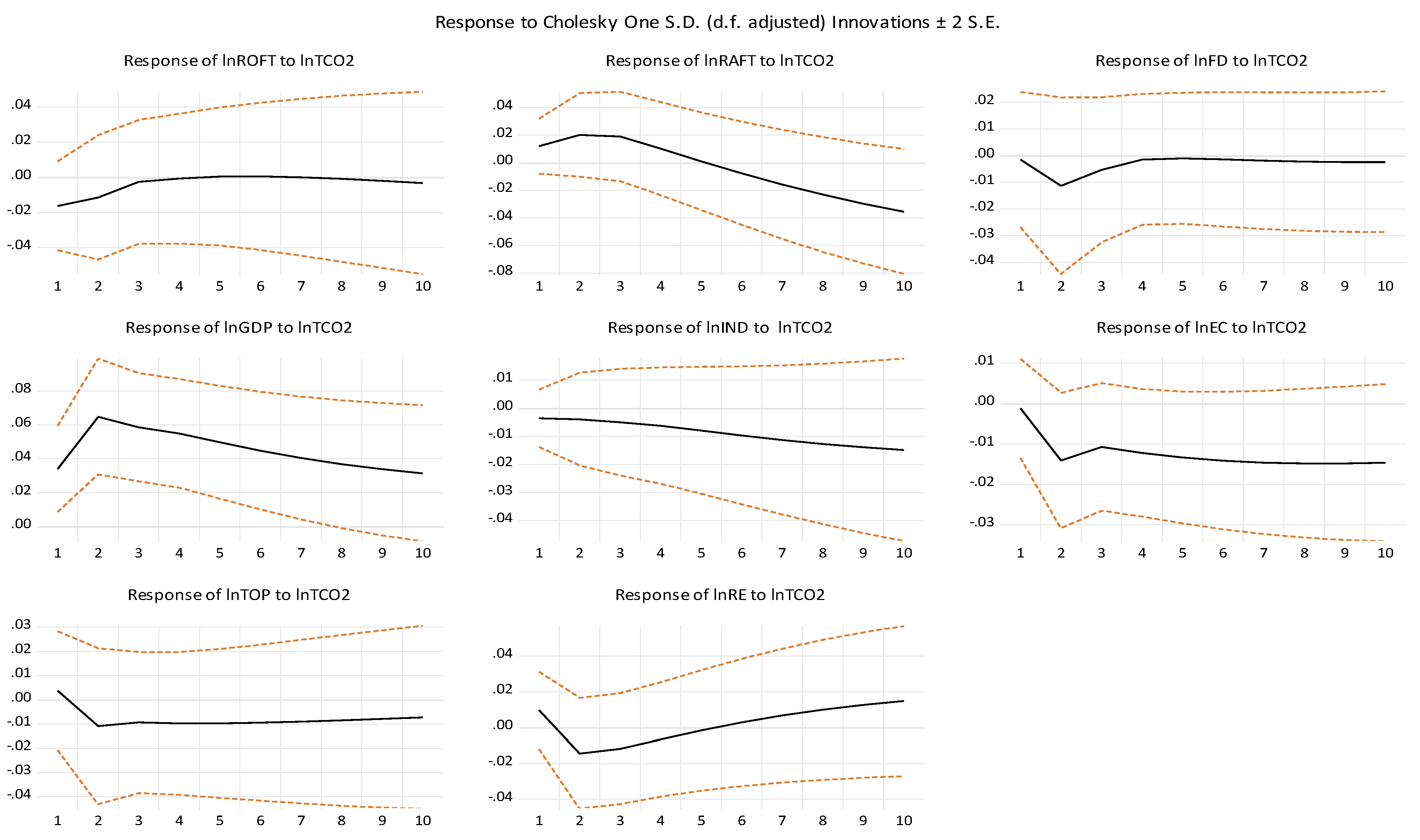
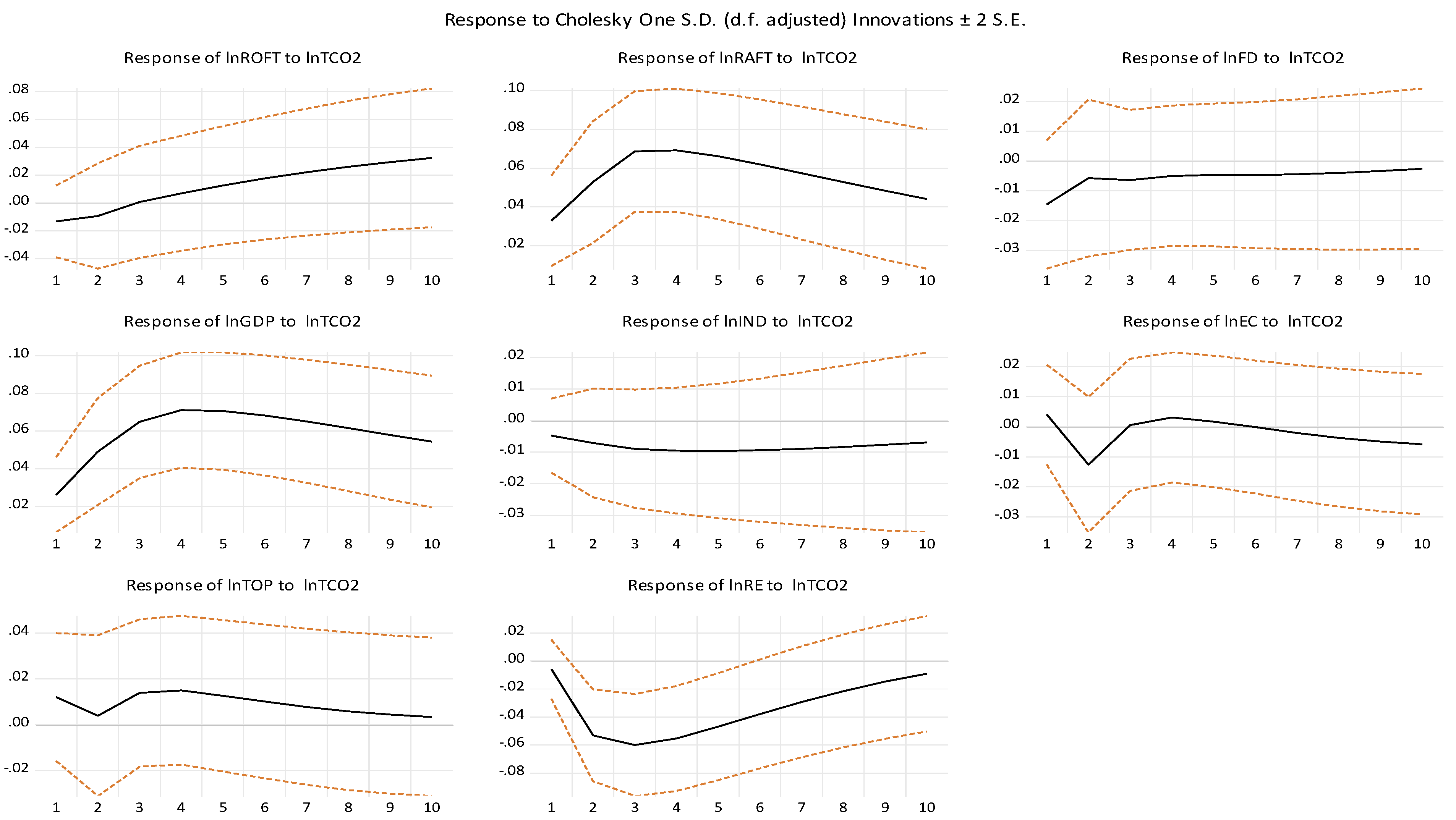
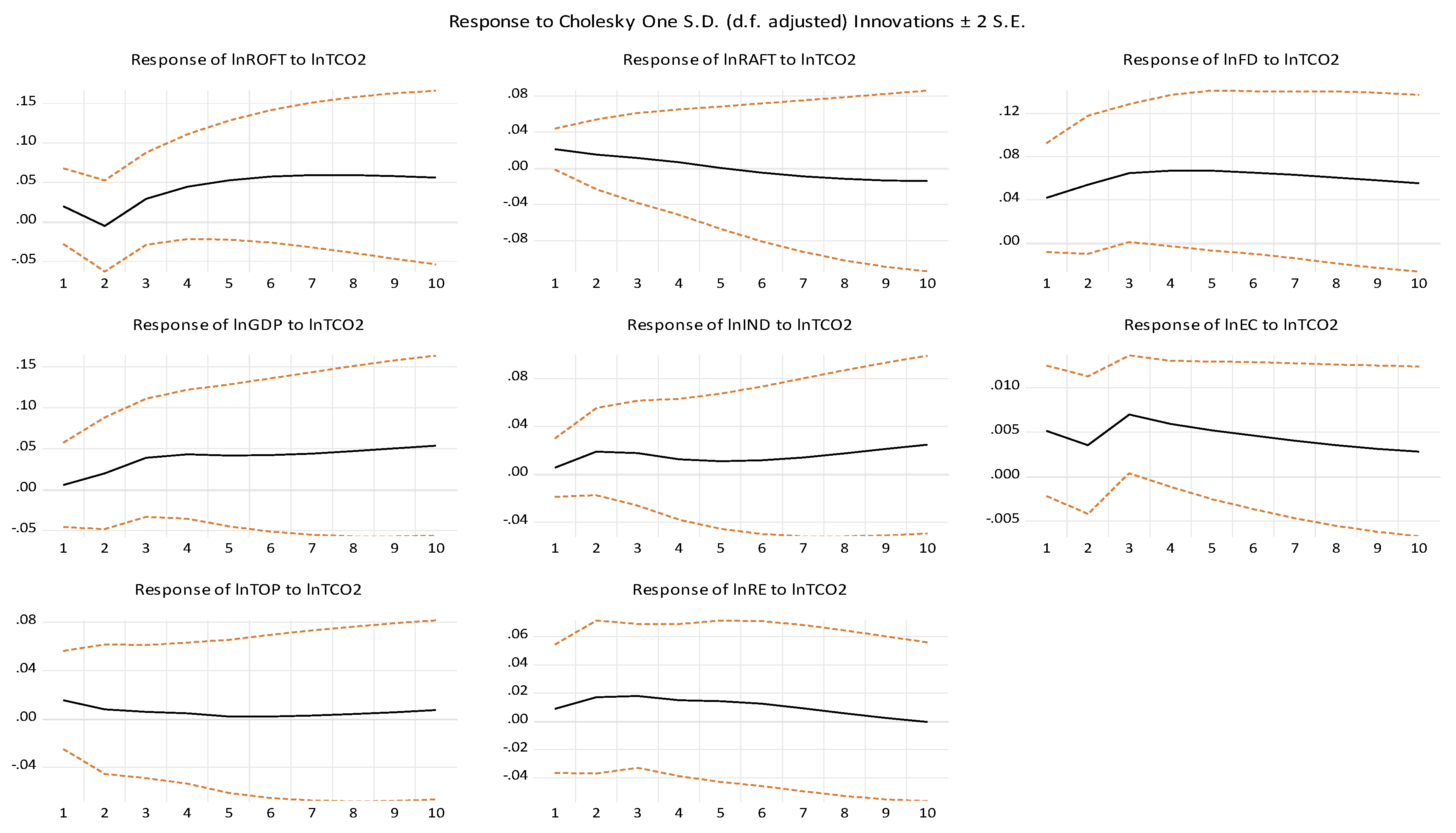
Figure 3.
IRF for all sample-LLc.
Figure 4.
IRF for European-LLc.
Figure 5.
IRF for Asian-LLc.
As reported in Table 10, The variance decomposition analysis of TCO2 reveals a dynamic temporal evolution and pronounced regional disparities that carry important implications for environmental policy. Across all regions, the contribution of TCO2's own shocks to its forecast variance declines significantly from 2023 to 2033, indicating that emissions become increasingly influenced by external factors over time. This trend is most pronounced in Asia, where self-influence falls from 100% to just 60.93%, compared to 90.18% globally and 84.93% in Europe, suggesting a growing complexity in the determinants of emissions. Simultaneously, the rising standard errors underscore heightened forecast uncertainty, further emphasizing the multifactorial nature of emissions. Regionally, the drivers of TCO₂ emissions differ markedly: in Europe, ROFT is the dominant external factor, with moderate contributions from EC and IND, while RE plays a marginal role. In contrast, Asia exhibits a broader and more balanced mix of contributors, with RAFT, GDP, FD, RE, and EC all exerting significant influence, reflecting the region’s diverse development paths and energy structures. The global sample presents an intermediate pattern, where RAFT, RE, FD, and TOP moderately explain emission variance. These findings suggest that effective decarbonization policies must be regionally tailored: Europe should focus on decarbonizing road freight and improving industrial energy efficiency, while Asia requires a multifaceted strategy involving rail modernization, green finance, renewable energy expansion, and economic decoupling. Globally, a coordinated policy mix targeting transport, energy, and financial systems is essential to drive emissions reductions. Overall, the analysis underscores the decreasing dominance of historical emission patterns and the growing role of sectoral and economic dynamics, highlighting the necessity for adaptive, region-specific approaches to climate governance.
5. Conclusion and Policy Implications
The study explores the dynamic impact of logistic operations, financial development, fossil fuel energy consumption, renewable energy consumption and industrialization on transport-based carbon dioxide emissions in landlocked countries across Europe and Asia. Despite a growing body of literature on the causal relationship between transport emissions and indicators for sustainable transportation in recent years, no previous study has explored this specific interrelationship. The aim of this study is to address this research gap by investigating the causal nexus between transport-related CO2 emissions, economic growth, road freight transports, rail freight transport, industry, trade openness, fossil fuel energy consumption, financial development, and renewable energy consumption in 11 landlocked countries from 1990 to 2022.
The findings of the PMG estimation for all sample landlocked countries demonstrate that rail freight transport is highly significant and has a negative relationship with TCO2. The result means that a percentage point increase in rail freight transport will cause TCO2 to decrease by 0.690% in the long-run. Industry, energy consumption, and trade openness variables also reveal a negative relationship with TCO2 in the long-run. This means that a percentage point increase in IND, EC, and TOP will cause TCO2 to decrease by 1.104%, 3.362%, and 0.394%, respectively. There is a positive but insignificant relationship between road freight transports, renewable energy consumption, and TCO2 in the long-run. On conclusion for the finding of the All Sample, economic growth and financial development are the main causes of environmental degradation in the transport sector. More interestingly, rail freight transport, industry, trade openness, and fossil fuel energy consumption have a remarkable negative impact on transport carbon emissions. The findings of the PMG estimation for the European sample of landlocked countries demonstrate that ROFT, IND, and RE significantly increase TCO2 in the long-run. When these variables grow by 1%, transport carbon dioxide emissions increase by 0.874%, 1.327%, and 0.368%, respectively. However, the impact of FD, GDP, and TOP on TCO2 emissions is significantly negative. The findings of the PMG estimation for the Asia sample of landlocked countries demonstrate that all the estimated variable coefficients are significant at the 1% level, except for TOP, which has a positive but insignificant impact on TCO2. Furthermore, the findings reveal that ROFT, FD, GDP, RE, and EC increase TCO2 in the long term; however, RAFT and IND decrease TCO2. Furthermore, the error correction terms for all sample countries, Europe, and Asia are found to be negative and significant. Robustness checks using FMOLS and DOLS confirm the long-term significance of the majority of explanatory variables, highlighting the validity of the PMG findings. All models exhibit negative and statistically significant error correction factors, hence affirming the presence of long-term equilibrium relationships. The table below presents a Summary of PMG, FMOLS, and DOLS. The findings of this paper carry several important implications for policymakers and strategies in LLcs that can be implemented to tackle the challenges faced and improve their logistics connectivity:
• Invest in Rail Infrastructure: Given that rail freight transport substantially decreases total CO₂ emissions over time, landlocked nations should prioritize the expansion and modernization of rail networks to transition freight from road-based transport systems.
• Diversify Energy Sources: While the effects of renewable energy differ by region, sustained investment in renewable infrastructure, like electrified railroads and biofuelcompatible transportation systems, can facilitate sustainable mobility.
• Promote Trade Liberalization and Industrial Efficiency: The inverse correlation between trade openness and TCO₂ indicates that participation in global markets, coupled with effective logistics, might improve environmental outcomes. Advocating for sustainable industrial policies is equally essential.
• Augment Regional Collaboration: Landlocked nations ought to capitalize on regional trade accords and collaborative infrastructure initiatives to enhance connectivity, optimize border processes, and ease access to global markets.
• Advocate for Technology and Innovation: Digital technology for supply chain optimization, real-time tracking, and customs automation can markedly improve logistics efficiency while minimizing emissions.
• Capacity Building and Regulatory Harmonization: Enhancing human capital and aligning customs and transportation rules with worldwide standards will facilitate effective and sustainable logistics systems.
This study possesses specific limitations that require attention in subsequent research. First ,the study excludes landlocked nations in Africa and the Americas due to data availability, hence constraining the worldwide applicability of its conclusions. Subsequent study should endeavor to include these regions to augment the thoroughness of the investigation. Secondly, essential governance-related issues, including political stability, institutional quality, and regulatory frameworks, are overlooked, despite their potential impact on policy execution and environmental results. Third, the study focuses on carbon dioxide emissions, neglecting other crucial environmental indicators such as nitrous oxide, sulfur dioxide, and ecological footprints, which are crucial for a comprehensive evaluation of environmental degradation. The analysis focuses exclusively on road and rail freight transport, disregarding other pertinent modes such as air, inland waterways, and passenger transport, which could substantially influence emissions profiles. The absence of comparison study with coastal states constrains the contextual comprehension of the distinct difficulties and opportunities encountered by landlocked countries. The dependence on annual data may obscure short-term variations and the direct effects of policy actions; hence, subsequent research should utilize higher-frequency or event-driven datasets. Minimizing these limitations will augment the profundity and pertinence of forthcoming studies and facilitate more efficacious, evidence-driven policymaking for sustainable transportation in landlocked countries .
References
- Fan, W.; Hao, Y. An empirical research on the relationship amongst renewable energy consumption, economic growth and foreign direct investment in China. Renewable energy 2020, 146, 598–609. [Google Scholar] [CrossRef]
- Timilsina, G.R.; Shrestha, A. Transport sector CO2 emissions growth in Asia: Underlying factors and policy options. Energy policy 2009, 37, 4523–4539. [Google Scholar] [CrossRef]
- Maryam, J.; Mittal, A.; Sharma, V. (2017). CO2 emissions, energy consumption and economic growth in BRICS: an empirical analysis. [CrossRef]
- Cook, D.; Davíðsdóttir, B. An appraisal of interlinkages between macro-economic indicators of economic well-being and the sustainable development goals. Ecological Economics 2021, 184, 106996. [Google Scholar] [CrossRef]
- Jensen, M.F. (2020). How Could Trade Measures Being Considered to Mitigate Climate Change Affect LDC Exports?. World Bank Policy Research Working Paper No. 9419.
- Nnene, O.A.; Senshaw, D.; Zuidgeest, M.; Mwaura, O.; Yitayih, Y. Developing Low-Carbon Pathways for the Transport Sector in Ethiopia. Climate 2025, 13, 96. [Google Scholar] [CrossRef]
- Ofélia de Queiroz, F.A.; Morte, I.B. B.; Borges, C.L.; Morgado, C.R.; de Medeiros, J.L. Beyond clean and affordable transition pathways: A review of issues and strategies to sustainable energy supply. International Journal of Electrical Power & Energy Systems 2024, 155, 109544. [Google Scholar] [CrossRef]
- Nathaniel, S.; Nwodo, O.; Adediran, A.; Sharma, G.; Shah, M.; Adeleye, N. Ecological footprint, urbanization, and energy consumption in South Africa: including the excluded. Environmental Science and Pollution Research 2019, 26, 27168–27179. [Google Scholar] [CrossRef]
- Raza, S.A.; Shah, N.; Sharif, A. Time frequency relationship between energy consumption, economic growth and environmental degradation in the United States: Evidence from transportation sector. Energy 2019, 173, 706–720. [Google Scholar] [CrossRef]
- Wada, I.; Faizulayev, A.; Bekun, F.V. Exploring the role of conventional energy consumption on environmental quality in Brazil: Evidence from cointegration and conditional causality. Gondwana Research 2021, 98, 244–256. [Google Scholar] [CrossRef]
- Destek, M.A. (2019). Financial development and environmental degradation in emerging economies. Energy and environmental strategies in the era of globalization, 115-132. [CrossRef]
- Ahmad, M.; Ahmed, Z.; Yang, X.; Hussain, N.; Sinha, A. Financial development and environmental degradation: do human capital and institutional quality make a difference? Gondwana Research 2022, 105, 299–310. [Google Scholar] [CrossRef]
- Baloch, M.A.; Zhang, J.; Iqbal, K.; Iqbal, Z. The effect of financial development on ecological footprint in BRI countries: evidence from panel data estimation. Environmental Science and Pollution Research 2019, 26, 6199–6208. [Google Scholar] [CrossRef]
- Al-Mulali, U.; Sab, C.N.B.C. The impact of energy consumption and CO2 emission on the economic growth and financial development in the Sub Saharan African countries. Energy 2012, 39, 180–186. [Google Scholar] [CrossRef]
- Gursoy-Haksevenler, B.H.; Atasoy-Aytis, E.; Dilaver, M.; Yalcinkaya, S.; Findik-Cinar, N.; Kucuk, E. ...& Yetis, U. A strategy for the implementation of water-quality-based discharge limits for the regulation of hazardous substances. Environmental Science and Pollution Research 2021, 28, 24706–24720. [Google Scholar] [CrossRef] [PubMed]
- Vidyarthi, H. An econometric study of energy consumption, carbon emissions and economic growth in South Asia: 1972-2009. World Journal of Science, technology and sustainable Development 2014, 11, 182–195. [Google Scholar] [CrossRef]
- Hassan, K.; Salim, R. Population ageing, income growth and CO2 emission: empirical evidence from high income OECD countries. Journal of Economic Studies 2015, 42, 54–67. [Google Scholar] [CrossRef]
- Ahmad, A.; Zhao, Y.; Shahbaz, M.; Bano, S.; Zhang, Z.; Wang, S.; Liu, Y. Carbon emissions, energy consumption and economic growth: An aggregate and disaggregate analysis of the Indian economy. Energy Policy 2016, 96, 131–143. [Google Scholar] [CrossRef]
- Mohammed, K.S.; Tiwari, S.; Ferraz, D.; Shahzadi, I. Assessing the EKC hypothesis by considering the supply chain disruption and greener energy: findings in the lens of sustainable development goals. Environmental Science and Pollution Research 2023, 30, 18168–18180. [Google Scholar] [CrossRef]
- Bölük, G.; Mert, M. Fossil & renewable energy consumption, GHGs (greenhouse gases) and economic growth: Evidence from a panel of EU (European Union) countries. Energy 2014, 74, 439–446. [Google Scholar] [CrossRef]
- Jebli, M.B.; Youssef, S.B.; Ozturk, I. Testing environmental Kuznets curve hypothesis: The role of renewable and non-renewable energy consumption and trade in OECD countries. Ecological indicators 2016, 60, 824–831. [Google Scholar] [CrossRef]
- Bilgili, F.; Koçak, E.; Bulut, Ü. The dynamic impact of renewable energy consumption on CO2 emissions: a revisited Environmental Kuznets Curve approach. Renewable and Sustainable Energy Reviews 2016, 54, 838–845. [Google Scholar] [CrossRef]
- Zoundi, Z. CO2 emissions, renewable energy, and the Environmental Kuznets Curve, a panel cointegration approach. Renewable Energy 2018, 129, 486–493. [Google Scholar] [CrossRef]
- Hu, H.; Xie, N.; Fang, D.; Zhang, X. The role of renewable energy consumption and commercial services trade in carbon dioxide reduction: Evidence from 25 developing countries. Applied energy 2018, 211, 1229–1244. [Google Scholar] [CrossRef]
- Sharif, A.; Raza, S.A.; Ozturk, I.; Afshan, S. The dynamic relationship of renewable and nonrenewable energy consumption with carbon emission: a global study with the application of heterogeneous panel estimations. Renewable energy 2019, 133, 685–691. [Google Scholar] [CrossRef]
- Raihan, A.; Rashid, M.; Voumik, L.C.; Akter, S.; Esquivias, M.A. The dynamic impacts of economic growth, financial globalization, fossil fuel, renewable energy, and urbanization on load capacity factor in Mexico. Sustainability 2023, 15, 13462. [Google Scholar] [CrossRef]
- Wang, Z.; Pham, T.L. H.; Sun, K.; Wang, B.; Bui, Q.; Hashemizadeh, A. The moderating role of financial development in the renewable energy consumption-CO2 emissions linkage: the case study of Next-11 countries. Energy 2022, 254, 124386. [Google Scholar] [CrossRef]
- Murshed, M.; Rashid, S.; Ulucak, R.; Dagar, V.; Rehman, A.; Alvarado, R.; Nathaniel, S.P. (2022). Mitigating energy production-based carbon dioxide emissions in Argentina: the roles of renewable energy and economic globalization. Environmental Science and Pollution Research, 1-20. [CrossRef]
- Zahoor, A.; Mehr, F.; Mao, G.; Yu, Y.; Sápi, A. (2023). The carbon neutrality feasibility of worldwide and in China's transportation sector by E-car. [CrossRef]
- Fan, W.; Hao, Y. An empirical research on the relationship amongst renewable energy consumption, economic growth and foreign direct investment in China. Renewable energy 2020, 146, 598–609. [Google Scholar] [CrossRef]
- Gu, Z.; Gao, Y.; Li, C. (2013, June). An empirical research on trade liberalization and CO2 emissions in China. In International Conference on Education Technology and Information System (ICETIS 2013) (pp. 243–246). [CrossRef]
- Akın, C.S. The impact of foreign trade, energy consumption and income on CO2 emissions. International Journal of Energy Economics and Policy 2014, 4, 465–475. [Google Scholar]
- Hakimi, A.; Hamdi, H. Trade liberalization, FDI inflows, environmental quality and economic growth: a comparative analysis between Tunisia and Morocco. Renewable and Sustainable Energy Reviews 2016, 58, 1445–1456. [Google Scholar] [CrossRef]
- Ling, T.Y.; Ab-Rahim, R.; Mohd-Kamal, K.A. Trade openness and environmental degradation in asean-5 countries. International Journal of Academic Research in Business and Social Sciences 2020, 10, 691–707. [Google Scholar] [CrossRef]
- Boutabba, M.A. The impact of financial development, income, energy and trade on carbon emissions: evidence from the Indian economy. Economic Modelling 2014, 40, 33–41. [Google Scholar] [CrossRef]
- Naranpanawa, A. (2011). Does Trade Openness Promote Carbon Emissions? Empirical Evidence from Sri Lanka. In The Empirical Economics Letters (Vol. 10, Issue 10) [Journal-article].
- Ertugrul, H.M.; Cetin, M.; Seker, F.; Dogan, E. The impact of trade openness on global carbon dioxide emissions: Evidence from the top ten emitters among developing countries. Ecological Indicators 2016, 67, 543–555. [Google Scholar] [CrossRef]
- Dogan, E.; Turkekul, B. CO 2 emissions, real output, energy consumption, trade, urbanization and financial development: testing the EKC hypothesis for the USA. Environmental Science and Pollution Research 2016, 23, 1203–1213. [Google Scholar] [CrossRef] [PubMed]
- Zamil, A.M.; Furqan, M.; Mahmood, H. Trade openness and CO2 emissions nexus in Oman. Entrepreneurship and Sustainability Issues 2019, 7, 1319. [Google Scholar] [CrossRef] [PubMed]
- Rahman, M.M.; Saidi, K.; Mbarek, M.B. (2020b). Economic growth in South Asia: the role of CO2 emissions, population density and trade openness. Heliyon, 6(5). [CrossRef]
- Yu, C.; Nataliia, D.; Yoo, S.J.; Hwang, Y.S. Does trade openness convey a positive impact for the environmental quality? Evidence from a panel of CIS countries. Eurasian Geography and Economics 2019, 60, 333–356. [Google Scholar] [CrossRef]
- Jun, W.; Mahmood, H.; Zakaria, M. Impact of trade openness on environment in China. Journal of Business Economics and Management 2020, 21, 1185–1202. [Google Scholar] [CrossRef]
- Adams, S.; Klobodu, E.K.M. Financial development, control of corruption and CO2 emissions: Evidence from African countries. Energy Economics 2017, 63, 209–216. [Google Scholar] [CrossRef]
- Achour, H.; Belloumi, M. Investigating the causal relationship between transport infrastructure, transport energy consumption and economic growth in Tunisia. Renewable and Sustainable Energy Reviews 2016, 56, 988–998. [Google Scholar] [CrossRef]
- Neves, S.A.; Marques, A.C.; Fuinhas, J.A. Is energy consumption in the transport sector hampering both economic growth and the reduction of CO2 emissions? A disaggregated energy consumption analysis. Transport policy 2017, 59, 64–70. [Google Scholar] [CrossRef]
- Song, M.; Wu, N.; Wu, K. Energy consumption and energy efficiency of the transportation sector in Shanghai. Sustainability 2014, 6, 702–717. [Google Scholar] [CrossRef]
- Murtishaw, S.; Schipper, L. Disaggregated analysis of US energy consumption in the 1990s: evidence of the effects of the internet and rapid economic growth. Energy Policy 2001, 29, 1335–1356. [Google Scholar] [CrossRef]
- Linton, C.; Grant-Muller, S.; Gale, W.F. Approaches and techniques for modelling CO2 emissions from road transport. Transport Reviews 2015, 35, 533–553. [Google Scholar] [CrossRef]
- Saidi, S.; Hammami, S. Modeling the causal linkages between transport, economic growth and environmental degradation for 75 countries. Transportation Research Part D: Transport and Environment 2017, 53, 415–427. [Google Scholar] [CrossRef]
- Shafique, M.; Azam, A.; Rafiq, M.; Luo, X. Evaluating the relationship between freight transport, economic prosperity, urbanization, and CO2 emissions: Evidence from Hong Kong, Singapore, and South Korea. Sustainability 2020, 12, 10664. [Google Scholar] [CrossRef]
- Carvalho, N.; Chaim, O.; Cazarini, E.; Gerolamo, M. Manufacturing in the fourth industrial revolution: A positive prospect in Sustainable Manufacturing. Procedia Manufacturing 2018, 21, 671–678. [Google Scholar] [CrossRef]
- Wang, F.; Shackman, J.; Liu, X. Carbon emission flow in the power industry and provincial CO2 emissions: Evidence from cross-provincial secondary energy trading in China. Journal of Cleaner Production 2017, 159, 397–409. [Google Scholar] [CrossRef]
- Abou-Ali, H.; Abdelfattah, Y.M.; Adams, J. (2016, April). Population dynamics and carbon emissions in the arab region: An extended stirpat II model. In Economic Research Forum Working Papers (Vol. 988).
- Rafiq, S.; Salim, R.; Apergis, N. Agriculture, trade openness and emissions: an empirical analysis and policy options. Australian Journal of Agricultural and Resource Economics 2016, 60, 348–365. [Google Scholar] [CrossRef]
- Nejat, P.; Jomehzadeh, F.; Taheri, M.M.; Gohari, M.; Majid, M.Z. A. A global review of energy consumption, CO2 emissions and policy in the residential sector (with an overview of the top ten CO2 emitting countries). Renewable and sustainable energy reviews 2015, 43, 843–862. [Google Scholar] [CrossRef]
- Tian, X.; Chang, M.; Shi, F.; Tanikawa, H. How does industrial structure change impact carbon dioxide emissions? A comparative analysis focusing on nine provincial regions in China. Environmental Science & Policy 2014, 37, 243–254. [Google Scholar] [CrossRef]
- Salim, R.A.; Shafiei, S. Urbanization and renewable and non-renewable energy consumption in OECD countries: An empirical analysis. Economic Modelling 2014, 38, 581–591. [Google Scholar] [CrossRef]
- Cherniwchan, J. Economic growth, industrialization, and the environment. Resource and Energy Economics 2012, 34, 442–467. [Google Scholar] [CrossRef]
- Shahbaz, M.; Uddin, G.S.; Rehman, I.U.; Imran, K. Industrialization, electricity consumption and CO2 emissions in Bangladesh. Renewable and Sustainable Energy Reviews 2014, 31, 575–586. [Google Scholar] [CrossRef]
- Asumadu-Sarkodie, S.; Owusu, P.A. Energy use, carbon dioxide emissions, GDP, industrialization, financial development, and population, a causal nexus in Sri Lanka: With a subsequent prediction of energy use using neural network. Energy Sources, Part B: Economics, Planning, and Policy 2016, 11, 889–899. [Google Scholar] [CrossRef]
- Asumadu-Sarkodie, S.; Owusu, P. (2017). Carbon dioxide emissions, GDP per capita, industrialization and population: An evidence from Rwanda. Environmental engineering research, 22(1). [CrossRef]
- Appiah, K.; Du, J.; Yeboah, M.; Appiah, R. Causal relationship between industrialization, energy intensity, economic growth and carbon dioxide emissions: recent evidence from Uganda. International Journal of Energy Economics and Policy 2019, 9, 237–245. [Google Scholar] [CrossRef]
- Anwar, N.; Elfaki, K.E. Examining the Relationship Between Energy Consumption, Economic Growth and Environmental Degradation in Indonesia: Do Capital and Trade Openness Matter? . International Journal of Renewable Energy Development 2021, 10, 769. [Google Scholar] [CrossRef]
- Nasrollahi, Z.; Hashemi, M.S.; Bameri, S.; Mohamad Taghvaee, V. Environmental pollution, economic growth, population, industrialization, and technology in weak and strong sustainability: using STIRPAT model. Environment, Development and Sustainability 2020, 22, 1105–1122. [Google Scholar] [CrossRef]
- International Energy Agency (IEA). (2024). Les émissions de carbone du secteur de l'énergie.
- Pesaran, M.H.; Ullah, A.; Yamagata, T. A bias-adjusted LM test of error cross-section independence. The Econometrics Journal 2008, 11, 105–127. [Google Scholar] [CrossRef]
- Pesaran, M.H. (2007), A simple panel unit root test in the presence of cross-section dependence. Journal of Applied Econometrics 22, 265-312. [CrossRef]
- Swamy, P.A. (1970). Efficient inference in a random coefficient regression model. Econometrica: Journal of the Econometric Society, 311-323. [CrossRef]
- Pedroni, P. (2004), Panel cointegration: A symptotic and finite sample properties of pooled time series tests with an application to the PPP hypothesis. Economic Theory 20, 597-625. [CrossRef]
- Kao, C. Spurious regression and residual-based tests for cointegration in panel data. Journal of econometrics 1999, 90, 1–44. [Google Scholar] [CrossRef]
- Pedroni, P. (2001). Fully modified OLS for heterogeneous cointegrated panels. In Nonstationary panels, panel cointegration, and dynamic panels (pp. 93–130). Emerald Group Publishing Limited. [CrossRef]
- Mark, N.C.; Sul, D. Nominal exchange rates and monetary fundamentals: evidence from a small post-Bretton Woods panel. Journal of international economics 2001, 53, 29–52. [Google Scholar] [CrossRef]
- Álvarez, I.C.; Barbero, J.; Rodríguez-Pose, A.; Zofío, J.L. Does institutional quality matter for trade? Institutional conditions in a sectoral trade framework. World Development 2018, 103, 72–87. [Google Scholar] [CrossRef]
- Dumitrescu, E.I.; Hurlin, C. Testing for Granger non-causality in heterogeneous panels. Economic modelling 2012, 29, 1450–1460. [Google Scholar] [CrossRef]
- Pesaran, M.H.; Ullah, A.; Yamagata, T. (2008), A bias-adjusted LM test of error cross-section independence. The Econometrics Journal, 11, 105-127. [CrossRef]
- Zhen You, Lei Li b, Muhammad Waqas (2024). How do information and communication technology, human capital and renewable energy affect CO2 emission; New insights from BRI countries. 10, e26-481. [CrossRef]
- Hasanov, F.J.; Mukhtarov, S.; Suleymanov, E. The role of renewable energy and total factor productivity in reducing CO2 emissions in Azerbaijan. Fresh insights from a new theoretical framework coupled with Autometrics. Energy Strategy Reviews 2023, 47, 101079. [Google Scholar] [CrossRef]
- Lopez, L.; Weber, S. Testing for Granger causality in panel data. The Stata Journal 2017, 17, 972–984. [Google Scholar] [CrossRef]
- Khan, H.U. R.; Siddique, M.; Zaman, K.; Yousaf, S.U.; Shoukry, A.M.; Gani, S. . & Saleem, H. The impact of air transportation, railways transportation, and port container traffic on energy demand, customs duty, and economic growth: Evidence from a panel of low-, middle-, and high-income countries. Journal of Air Transport Management 2018, 70, 18–35. [Google Scholar] [CrossRef]
- McKinnon, A. (2018). Decarbonizing Logistics: Distributing Goods in a Low Carbon World. Kogan Page Publishers.
- International Energy Agency (IEA). (2021). Transport – Analysis. IEA, Paris.
- European Environment Agency (EEA). Transport emissions of greenhouse gases. EEA, Copenhagen.
- Arbolino, R.; Carlucci, F.; De Simone, L.; Ioppolo, G.; Yigitcanlar, T. (2018). The policy diffusion of environmental performance in the European countries. Ecological Indicators 2019, 89, 130–138. [Google Scholar] [CrossRef]
- Ćosović; E; Mihajlović; I; SpasojevićBrkić, V. (2024). IMPACT OF FUEL CONSUMPTION ON CO2 EMISSIONS IN ROAD TRANSPORT IN EUROPEAN COUNTRIES. In Proceedings of the XIV International Conference-Industrial Engineering and Environmental Protection (IIZS 2024) (pp. 380–387). Zrenjanin: Technical Faculty" Mihajlo Pupin". [CrossRef]
- Saha, R.C.; Sabur, H.M. A.; Saif, T.M. R. Environmental sustainability of inland freight transportation Systems in Bangladesh. International Supply Chain Technology Journal 2023, 9, 1–21. [Google Scholar] [CrossRef]
- Rabbi, M.F.; Abdullah, M. Fossil fuel CO2 emissions and economic growth in the Visegrád region: A study based on the environmental Kuznets curve hypothesis. Climate 2024, 12, 115. [Google Scholar] [CrossRef]
- Holappa, L. A general vision for reduction of energy consumption and CO2 emissions from the steel industry. Metals 2020, 10, 1117. [Google Scholar] [CrossRef]
- Lei, R.; Feng, S.; Lauvaux, T. Country-scale trends in air pollution and fossil fuel CO2 emissions during 2001–2018: confronting the roles of national policies and economic growth. Environmental Research Letters 2020, 16, 014006. [Google Scholar] [CrossRef]
- Vo, N. (2024). Assessing the impact of feed-in tariffs and renewable portfolio standards on the development of solar photovoltaic in Vietnam–opportunities and challenges.
- Hariyani, H.F.; Prasetyo, D.G.; Van Ha, T.T.; Dam, B.H.; Nguyen, T.T. H. Unlocking CO2 emissions in East Asia Pacific-5 countries: Exploring the dynamics relationships among economic growth, foreign direct investment, trade openness, financial development and energy consumption. Journal of Infrastructure Policy and Development 2024, 8, 5639. [Google Scholar] [CrossRef]
- Nasrullah, N.; Husnain, M.I. U.; Khan, M.A. The dynamic impact of renewable energy consumption, trade, and financial development on carbon emissions in low-, middle-, and high-income countries. Environmental Science and Pollution Research 2023, 30, 56759–56773. [Google Scholar] [CrossRef]
Figure 1.
Analytical methodology flowchart
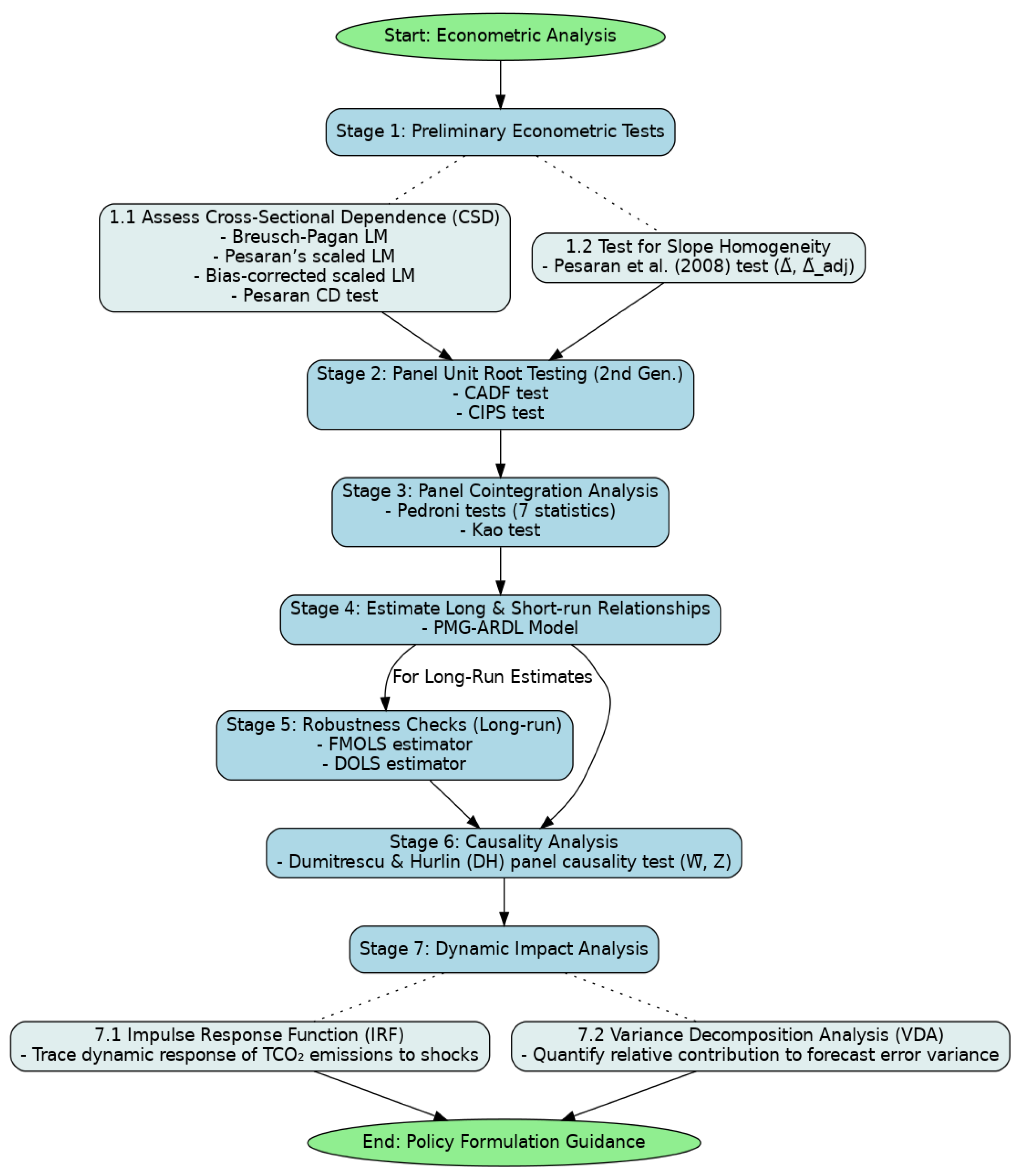
Figure 2.
Summary of causalities betweeen TCO2 and expalantory variables in all sample, European and Asian-LLc.
Figure 2.
Summary of causalities betweeen TCO2 and expalantory variables in all sample, European and Asian-LLc.
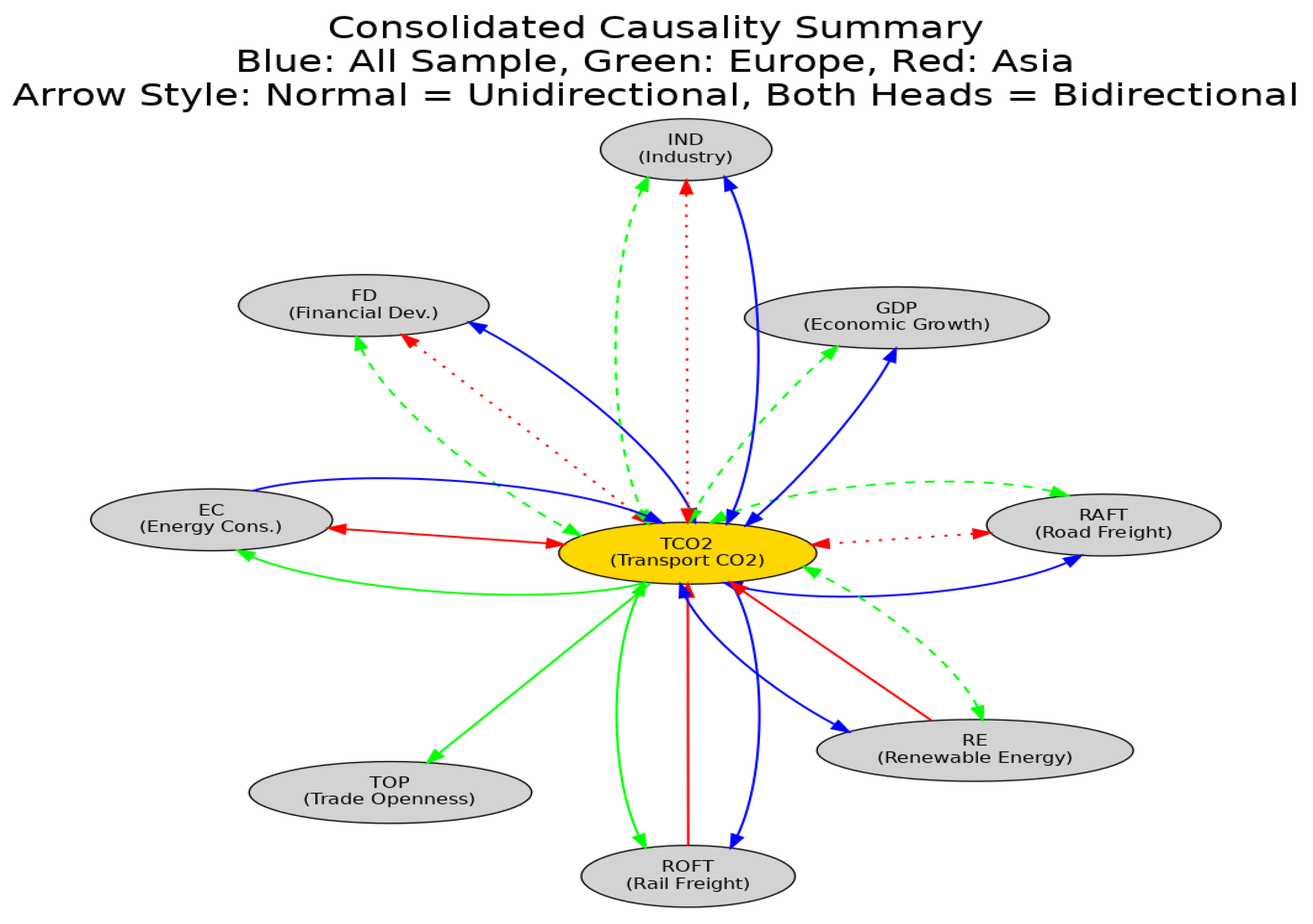
Table 1.
Description of the variables and data sources.
| Variables | Definitions | Measurements | Sources |
| TCO2 | Transport-related carbon dioxide emissions | % of total fuel combustion | IEA (2024)[65] |
| ROFT | road freight transports | millions of metric tons times kilometers traveled | WDI(2024) |
| RAFT | Rail freight transports | millions of metric tons times kilometers traveled | WDI(2024) |
| GDP | Gross Domestic Product | Current US$ | WDI(2024) |
| IND | Industry (including construction) | Current US$ | WDI(2024) |
| EC | Fossil fuel energy consumption | % of total energy consumption | WDI(2024) |
| TOP | Trade openness: Total trade in goods and services | Million US dollars | WDI(2024) |
| RE | Renewable energy consumption | % of total final energy consumption | WDI(2024) |
| FD | Financial development | Domestic credit to private sector (% of GDP) | WDI(2024) |
Source: Authors Elaboration.
Table 2.
Descriptive statistics.
| lnTCO2 | lnROFT | lnRAFT | lnFD | lnGDP | lnIND | lnEC | lnTOP | lnRE | |
| All sample-LLc | |||||||||
| Mean | 2.869 | 9.495 | 9.436 | 3.677 | 8.914 | 21.652 | 5.040 | 11.302 | 1.835 |
| Maximum | 4.224 | 12.115 | 12.648 | 5.194 | 11.803 | 25.988 | 11.833 | 14.105 | 3.951 |
| Minimum | 1.537 | 4.889 | 5.948 | 0.009 | 4.098 | 2.641 | 3.840 | 8.315 | -0.328 |
| Std. Dev. | 0.729 | 1.393 | 1.407 | 1.021 | 1.590 | 6.333 | 1.950 | 1.392 | 1.185 |
| Skewness | -0.008 | -0.924 | 0.249 | -0.901 | -0.065 | -2.515 | 2.657 | -0.157 | 0.001 |
| Kurtosis | 1.910 | 4.034 | 3.497 | 3.650 | 2.231 | 7.662 | 8.246 | 2.218 | 1.699 |
| Jarque-Bera | 16.384 | 61.949 | 6.840 | 50.627 | 8.385 | 648.806 | 769.191 | 9.781 | 23.326 23.326 |
| European-LLc | |||||||||
| Mean | 3.158 | 9.651 | 9.227 | 4.117 | 9.599 | 21.018 | 5.233 | 2.433 | 11.929 |
| Maximum | 4.232 | 11.460 | 11.230 | 5.227 | 11.803 | 26.122 | 11.833 | 3.951 | 14.105 14.105 |
| Minimum | 1.548 | 5.624 | 5.948 | 1.360 | 6.387 | 2.641 | 3.808 | -0.083 | 8.315 |
| Std. Dev. | 0.624 | 1.087 | 0.909 | 0.749 | 1.359 | 7.472 | 2.310 | 0.931 | 1.216 |
| Skewness | -0.231 | -1.304 | -0.662 | -1.135 | -0.265 | -1.949 | 2.045 | -0.520 | -0.759 |
| Kurtosis | 2.333 | 5.268 | 4.510 | 4.233 | 2.071 | 4.972 | 5.287 | 2.457 | 3.533 |
| Jarque-Bera | 6.329 | 114.989 | 38.841 | 64.322 | 10.999 | 183.834 | 211.394 | 13.283 13.283 | 24.925 24.925 |
| Asian-LLC | |||||||||
| Mean | 2.333 333 |
8.814 | 9.375 | 2.778 | 7.499 | 23.005 | 4.512 | 10.063 | 0.938 |
| Maximum | 3.626 | 12.115 | 12.648 | 4.369 | 9.538 | 25.070 | 4.612 | 11.960 11.960 | 2.876 |
| Minimum | 0.641 | 4.889 | 5.777 | 0.009 | 4.098 | 20.448 | 4.054 | 8.344 | -0.328 |
| Std. Dev. | 0.668 | 2.105 | 2.204 | 0.893 | 1.120 | 1.216 | 0.142 | 0.978 | 0.772 |
| Skewness | 0.201 | -0.352 | -0.027 | -0.734 | -0.118 | -0.259 | -1.515 | 0.143 | 0.815 |
| Kurtosis | 2.394 | 2.096 | 1.877 | 3.755 | 2.328 | 2.150 | 3.692 | 1.874 | 2.366 |
| Jarque-Bera | 2.905 | 7.219 | 6.946 | 15.013 | 2.783 | 5.450 | 53.183 | 7.419 | 16.847 16.847 |
Source: Author own calculation by using E-Views 12
Table 4.
Slope homogeneity test for All sample, European and Asian-LLc.
| All sample-LLc | Europeean-LLc | Asian-LLc | ||||
| Statistics | T-statistics | P-value | T-statistics | P-value | T-statistics | P-value |
| 12.255 | 0.0001*** | 17.698 | 0.0000*** | 12.084 | 0.0000*** | |
| 18.053 | 0.000*** | 12.292 | 0.0005*** | 16.115 | 0.0000*** | |
Notes: The Null hypothesis for slope homogeneity test is that slope coefficients are homogenous, *** denotes significant at 1% levels.
Table 5.
Second-generation Panel unit root tests.
| CIPS |
CADF |
|||
| Level | 1st Difference | Level | 1st Difference | |
| All Sample | ||||
| lnTCO2 | -2.273** | -5.774*** | -1.564 | -4.431*** |
| lnGDP | -3.476*** | -5.254*** | -2.557*** | -3.986*** |
| lnRAFT | -1.908 | -5.317*** | -1.935 | -4.101*** |
| lnROFT | -1.816 | -5.337*** | -1.454 | -4.059*** |
| lnFD | -1.788 | -5.175*** | -1.992 | -3.752*** |
| lnIND | -1.798 | -4.312*** | -2.402** | -3.647*** |
| lnTOP | -1.794 | -5.167*** | -1.687 | -4.230*** |
| lnEC | -1.371 | -5.276*** | -1.201 | -3.767*** |
| lnRE | -1.973 | -4.989*** | -2.110 | -3.326*** |
| Europe | ||||
| lnTCO2 | -3.269*** | -5.776*** | -2.469** | -4.315*** |
| lnGDP | -4.193*** | -5.933*** | -1.912 | -4.404*** |
| lnRAFT | -1,747 | -5.018*** | -1.742 | -3.717*** |
| lnROFT | -1.934 | -5.946*** | -2.228 | -4.133*** |
| lnFD | -1.640 | -5.053*** | -1.630 | -3.806*** |
| lnIND | -0.812 | -5.151*** | -1.067 | -4.322*** |
| lnTOP | -1.515 | -5.284*** | -1.651 | -3.478*** |
| lnEC | -2.077 | -5,365*** | -1.822 | -4.130*** |
| lnRE | -2.032 | -5.320*** | -1.536 | -4.119*** |
| Asia | ||||
| lnTCO2 | -2.856*** | -5.442*** | -2.131 | -4.589*** |
| lnGDP | -2.062 | -4.970*** | -2.229 | -4.223*** |
| lnRAFT | -1.832 | -5.696*** | -2.839** | -4.662*** |
| lnROFT | -1.913 | -5.539*** | -1.865 | -4.589*** |
| lnFD | -1.946 | -5.485*** | -2.766** | -4.172*** |
| lnIND | -1.742 | -4.845*** | -2.391* | -3.576*** |
| lnTOP | -1.896 | -5.454*** | -2.087 | -4.252*** |
| lnEC | -2.237* | -6.072*** | -1.690 | -4.757*** |
| lnRE | -2.551** | -5.272*** | -2.562** | -4.280*** |
Source: Author own calculation by using E-Views 12.Note: Null hypothesis indicates that time series are not stationary, *** , ** and * represent 1%, 5% and 10% significance level respectively.CIPS: Cross-sectionally Augmented IPS, CADF: Cross-sectionally Augmented Dicky-Fuller.
Table 6.
Results of cointegrations test for All sample, Europe and Asia.
| All sample-LLc | European-LLc | Asian-LLc | |||||
| Pedroni Residual Cointegration Test | |||||||
| Alternative hypothesis: common AR coefs. (within-dimension) | |||||||
| Statistic | P-value | Statistic | P-value | Statistic | P-value | ||
| Panel v-Statistic | -2.244 | 0.987 | -0.300 | 0.618 | -1.857 | 0.968 | |
| Panel rho-Statistic | 2.480 | 0.993 | 1.182 | 0.881 | 1.826 | 0.966 | |
| Panel PP-Statistic | -0.751 | 0.226 | -2.482 | 0.006*** | 0.321 | 0.626 | |
| Panel ADF-Statistic | -1.004 | 0.157 | -3.543 | 0.000*** | 0.537 | 0.704 | |
| Alternative hypothesis: individual AR coefs. (between-dimension) | |||||||
| Panel rho-Statistic | 2.983 | 0.998 | 2.054 | 0.980 | 2.229 | 0.987 | |
| Panel PP-Statistic | -2.265 | 0.011** | -2.165 | 0.015** | -0.892 | 0.186 | |
| Panel ADF-Statistic | -0.033 | 0.486 | -0.785 | 0.216 | 0.983 | 0.837 | |
| Kao Residual Cointegration Test | |||||||
| t-Statistic | Prob | t-Statistic | Prob | t-Statistic | Prob | ||
| ADF | -1.267 | 0.102 | -3.190 | 0.000*** | -4.745 | 0.000*** | |
Source: Author own calculation by using E-Views 12 . Note: ***, **, and * denote statistical significance level at 1%, 5%, and 10%, level, respectively.
Table 7.
The results of PMG-ARDL for full sample, Europe and Asia.
| All-sample-LLc | European-LLc | Asian-LLc | ||||
| Variables | Coef | p-value | Coef | p-value | Coef | p-value |
| Long run analysis | ||||||
| lnROFT | 0.053 | 0.568 | 0.874 | 0.000*** | 0.251 | 0.000*** |
| lnRAFT | -0.690 | 0.000*** | 0.017 | 0.658 | -0.806 | 0.000*** |
| lnFD | 0.650 | 0.000*** | -1.204 | 0.000*** | 0.535 | 0.000*** |
| lnGDP | 0.720 | 0.000*** | -0.355 | 0.000*** | 0.318 | 0.000*** |
| lnIND | -1.104 | 0.000*** | 1.327 | 0.000*** | -0.525 | 0.000*** |
| lnEC | -3.362 | 0.000*** | 0.303 | 0.318 | 12.595 | 0.000*** |
| lnTOP | -0.394 | 0.001*** | -0.208 | 0.000*** | 0.074 | 0.468 |
| lnRE | 0.176 | 0.129 | 0.368 | 0.000*** | 0.512 | 0.000*** |
| Short run analysis | ||||||
| Coint Eq (-1) | -0.108 | (0.053) ** | -0.121 | 0.024** | -0.410 | 0.025** |
| D (lnROFT) | 0.012 | (0.889) | -0.168 | 0.396 | -0.042 | 0.631 |
| D (lnRAFT) | 0.032 | (0.574) | -0.049 | 0.504 | 0.147 | 0.590 |
| D (lnFD) | -0.213 | (0.293) | 0.594 | 0.443 | 0.298 | 0.469 |
| D (lnGDP) | 0.037 | (0.368) | 0.030 | 0.661 | -0.276 | 0.014** |
| D (lnIND) | 0.062 | (0.635) | -0.062 | 0.712 | -0.125 | 0.675 |
| D (lnEC) | -0.303 | (0.579) | 0.071 | 0.908 | -6.755 | 0.273 |
| D (lnTOP) | 0.078 | (0.012) ** | -0.180 | 0.417 | -0.016 | 0.896 |
| D (lnRE) | 0.054 | (0.423) | 0.166 | 0.268 | -0.037 | 0.663 |
| C | 4.871 | (0.057) ** | -3.352 | 0.265 | -17.395 | 0.025* |
Source: Author own calculation by using E-Views 12 Note: *** and * shows statistical significant at 1%, 5% and 10% respectively. The model selection method used is the Akaike information criterion: Full sample selected model: ARDL(2, 1, 1, 1, 1, 1, 1, 1, 1); Europe selected model: ARDL(1, 2, 2, 2, 2, 2, 2, 2, 2); Asia selected model: ARDL(2, 2, 2, 2, 2, 2, 2, 2, 2). Note: *** and * shows statistical significant at 1%, 5% and 10% respectively. The model selection method used is the Akaike information criterion: Full sample selected model: ARDL(2, 1, 1, 1, 1, 1, 1, 1, 1); Europe selected model: ARDL(1, 2, 2, 2, 2, 2, 2, 2, 2); Asia selected model: ARDL(2, 2, 2, 2, 2, 2, 2, 2, 2).
Table 8.
FMOLS and DOLS estimates for All sample, European and Asian-LLc.
| All-Sample-LLc | European-LLc | Asian-LLc | ||||
| Variables | Coefficient | Coefficient | Coefficient | |||
| Fully Modified Ordinary Least Square (FMOLS) | ||||||
| Ln TCO2 Ln ROFT Ln RAFT Ln FD Ln GDP Ln IND Ln EC Ln TOP Ln RE |
- -0.019 (0.000)*** -0.243 (0.000)*** -0.202 (0.000)*** 0.382 (0.000)*** 0.066 (0.000)*** 0.119 (0.000)*** 0.030 (0.000)*** 0.098 (0.000)*** |
- 3.95E-05 (0.997) 0.027 (0,099)* -0.248 (0.000)*** 0.544 (0.000)*** -0.081 (0.000)*** -0.157 (0.000)*** 0.080 (0.000)*** 0.023 (0.000)*** |
- 0.164 (0.000)*** 0.154 (0.005)*** 0.171 (0.003)*** 0.293 (0.000)*** -0.305 (0.000)*** -0.473 (0.000)*** -0.249 (0.000)*** -0.419 (0.000)*** |
|||
| Dynamic Ordinary Least Square (DOLS) | ||||||
| Ln TCO2 Ln ROFT Ln RAFT Ln FD Ln GDP Ln IND Ln EC Ln TOP Ln RE |
- -0.665 (0.000)*** 1.319 (0.000)*** 2.059 (0.000)*** 0.848 (0.000)*** -0.218 (0.594) 0.423 (0.032)** 0.203(0.112) -2.070 (0.000)*** |
- -0.014 (0.764) 0.135 (0.006)*** -0.326 (0.003)*** 0.527 (0.000)*** -0.086 (0.001)*** -0.195 (0.003)*** 0.086 (0.107) 0.048 (0.429) |
- 0.391 (0.001)*** -0.252 (0.004)*** 0.255 (0.011)* 0.518 (0.000)*** -1.296 (0.000)*** 5.145 (0.000)*** 0.306 (0.025)* 0.289 (0.351) |
|||
Source: Author own calculation by using E-Views 12 Note : ***, **, and * denote statistical significance level at 1%, 5%, and 10%, level, respectively.
Table 9.
Dumitrescu Hurlin (DH) Panel Causality Tests.
| All sample-LLc | European-LLc | Asian-LLc | |||||||
| Null Hypothesis | W-stat | Zbar-stat | Probability | W-stat | Zbar-stat | Probability | W-stat | Zbar-stat | Probability |
| lnRAFT≠lnTCO2 | 5.231 | 2.075 | 0.037** | 17.468 | 3.410 | 0.000*** | 46.386 | 7.159 | 8.E-13*** |
| lnTCO2≠lnRAFT | 7.207 | 4.208 | 3.E-05*** | 25.300 | 6.407 | 1.E-10*** | 26.934 | 5.316 | 1.E-07*** |
| lnROFT≠lnTCO2 | 4.483 | 1.273 | 0.203 | 11.966 | 3.749 | 0.000*** | 24.519 | 2.776 | 0.005*** |
| lnTCO2≠lnROFT | 8.981 | 6.139 | 8.E-10*** | 15.924 | 2.819 | 0.004*** | 10.175 | -0.098 | 0.921 |
| lnFD ≠lnTCO2 | 8.405 | 5.543 | 3.E-08*** | 3.508 | 4.006 | 6.E-05*** | 92.597 | 16.422 | 0.000*** |
| lnTCO2 ≠lnFD | 4.920 | 1.758 | 0.0786* | 3.932 | 4.705 | 3.E-06*** | 34.068 | 4.690 | 3.E-06*** |
| lnGDP ≠lnTCO2 | 6.923 | 3.934 | 8.E-05*** | 4.780 | 2.936 | 0.003*** | 13.145 | 0.496 | 0.619 |
| lnTCO2 ≠lnGDP | 4.853 | 1.686 | 0.0917* | 4.536 | 2.662 | 0.007*** | 9.236 | -0.286 | 0.774 |
| lnIND ≠lnTCO2 | 9.886 | 6.939 | 4.E-12*** | 3.273 | 3.620 | 0.000*** | 23.052 | 10.099 | 0.000*** |
| lnTCO2 ≠lnIND | 6.256 | 3.098 | 0.001*** | 3.858 | 4.582 | 5.E-06*** | 9.759 | 2.884 | 0.003*** |
| lnEC ≠lnTCO2 | 2.568 | 3.062 | 0.002*** | 1.599 | -0.637 | 0.523 | 53.231 | 8.531 | 0.000*** |
| lnTCO2 ≠lnEC | 0.955 | -0.248 | 0.803 | 4.465 | 2.582 | 0.009** | 35.371 | 4.951 | 7.E-07*** |
| lnTOP ≠lnTCO2 | 3.847 | 0.455 | 0.648 | 16.776 | 0.191 | 0.847 | 7.075 | -0.719 | 0.471 |
| lnTCO2 ≠lnTOP | 2.984 | -0.394 | 0.693 | 41.008 | 2.809 | 0.005*** | 15.945 | 1.058 | 0.290 |
| lnRE ≠lnTCO2 | 2.456 | 2.828 | 0.004*** | 24.182 | 3.584 | 0.000*** | 34.954 | 4.868 | 1.E-06*** |
| lnTCO2 ≠lnRE | 2.033 | 1.959 | 0.050** | 27.921 | 4.575 | 5.E-06*** | 15.446 | 0.958 | 0.338 |
|
Summary of causalites : All sample-LLc : RAFT↔ TCO2 ; TCO2 → ROFT ; FD ↔ TCO2 ; GDP ↔ TCO2 ; IND ↔ TCO2 ; EC → TCO2 ; TCO2 ↔ RE European-LLc : ROFT ↔ TCO2 ; RAFT ↔ TCO2 ; FD ↔ TCO2 ; GDP ↔ TCO2 ; IND ↔ TCO2 ; TCO2 → EC ; TCO2→TOP ; RE ↔ TCO2 Asian-LLc : RAFT↔TCO2 ; ROFT→ TCO2 ; FD ↔ TCO2 ; IND ↔ TCO2 ; EC ↔ TCO2 ; RE → TCO2 Note: ***,** and * shows statistical significant at 1%, 5% and 10% level respectively, → indicate unidirectional causality, ↔ indicate bidirectional causality and ≠ denotes that A does not homogeneously cause B. | |||||||||
Source: Author own calculation by using E-Views 12.
Table 10.
Variance decomposition analysis.
| Period | S.E. | lnTCO2 | lnROFT | lnRAFT | lnFD | lnGDP | lnIND | lnEC | lnTOP | lnRE |
| All sample-LLc | ||||||||||
| 2023 | 0.101506 | 100.0000 | 0.000000 | 0.000000 | 0.000000 | 0.000000 | 0.000000 | 0.000000 | 0.000000 | 0.000000 |
| 2028 | 0.193542 | 96.70943 | 1.040579 | 0.348878 | 0.724071 | 0.174985 | 0.324044 | 0.011983 | 0.173929 | 0.492103 |
| 2033 | 0.251320 | 90.17627 | 1.196186 | 3.684687 | 1.324250 | 0.209753 | 0.426638 | 0.047857 | 0.994332 | 1.940026 |
| European-LLc | ||||||||||
| 2023 | 0.081614 | 100.0000 | 0.000000 | 0.000000 | 0.000000 | 0.000000 | 0.000000 | 0.000000 | 0.000000 | 0.000000 |
| 2028 | 0.164400 | 90.58908 | 4.520048 | 1.497820 | 0.089900 | 0.942239 | 1.426338 | 0.853628 | 0.017232 | 0.063720 |
| 2033 | 0.205835 | 84.92786 | 7.788997 | 1.408449 | 0.108510 | 1.238609 | 1.994292 | 2.019309 | 0.436806 | 0.077166 |
| Asian-LLc | ||||||||||
| 2023 | 0.226549 | 100.0000 | 0.000000 | 0.000000 | 0.000000 | 0.000000 | 0.000000 | 0.000000 | 0.000000 | 0.000000 |
| 2028 | 0.461080 | 74.87811 | 1.930243 | 9.988028 | 2.024419 | 3.634298 | 1.518210 | 0.992425 | 0.047586 | 4.986683 |
| 2033 | 0.549368 | 60.92547 | 1.783830 | 13.62304 | 6.345661 | 7.957332 | 1.651150 | 3.163423 | 0.250552 | 4.299539 |
Source: Author own calculation by using E-Views 12.
Disclaimer/Publisher’s Note: The statements, opinions and data contained in all publications are solely those of the individual author(s) and contributor(s) and not of MDPI and/or the editor(s). MDPI and/or the editor(s) disclaim responsibility for any injury to people or property resulting from any ideas, methods, instructions or products referred to in the content. |
© 2025 by the authors. Licensee MDPI, Basel, Switzerland. This article is an open access article distributed under the terms and conditions of the Creative Commons Attribution (CC BY) license (http://creativecommons.org/licenses/by/4.0/).
Copyright: This open access article is published under a Creative Commons CC BY 4.0 license, which permit the free download, distribution, and reuse, provided that the author and preprint are cited in any reuse.


