
Submitted:
11 June 2024
Posted:
11 June 2024
You are already at the latest version
Abstract
: Leveraging the sustainability of the power system market, researchers have developed various ML models for forecasting electricity demand. The LSSVM is well suited to handle complex non-linear power load series. However, the less optimal regularization parameter and the Gaussian kernel function in the LSSVM model have contributed to flawed forecasting accuracy and random generalization ability. Thus, these parameters of LSSVM need to be chosen appropriately using intelligent optimization algorithms. This study proposes a hybrid model based on the LSSVM optimized by the IBFOA for forecasting the daily electricity load in Peninsular Malaysia. The IBFOA for parameter optimization of LSSVM is introduced. The IBFOA based on the sine cosine equation is proposed to adjust the constant step size in the BFOA, which creates an imbalance between the exploration and exploitation during optimization. Finally, the load forecasting model based on LSSVM-IBFOA is constructed using MAPE as the objective function. Comparative analysis demonstrates the model, achieving the highest R2 (0.9880) and significantly reducing error metrics (MAPE, MAE, RMSE, MSE, NRMSE) compared to the baseline LSSVM (average reduction of 27.72% to 47.72%). Additionally, IBFOA exhibits faster convergence and higher accuracy compared to BFOA, highlighting the accuracy of LSSVM-IBFOA for short-term load forecasting.
Keywords:
Electricity load forecasting
; Least square support vector machine (LSSVM)
; Improved Bacterial foraging optimization algorithm (IBFOA)
; hybrid model
; machine learning (ML)
1. Introduction
Energy is a cornerstone of sustainable development for nations worldwide. Over the past decade, there has been an increase in global energy demand. Malaysia, among the most highly developed states of the Southeast Asia region, has projected its total final energy consumption to almost double by 2050, driven by an increasing urban population and economic growth. The energy demand in Malaysia has correlated with gross domestic product (GDP) growth as the economy depends on energy-intensive industries such as manufacturing. However, the previous COVID-19 pandemic’s impact disrupted the energy demand which has lower the GDP growth. In 2020, Malaysia’s GDP experienced a significant decline of 5.54%, leading to a corresponding decrease in electricity generation (2.4%) and total final energy consumption (-0.5%), particularly within the industrial sector compared to 2019. Therefore, the government has planned an economic recovery program to stimulate the economy, with an expected GDP growth of 3.44% per year from 2020 until 2030 [1]. The growth illustrates the increasing energy demand needed to achieve the goal. Malaysia’s energy landscape is projected to undergo a significant transformation, balancing anticipated demand growth with a resolute transition towards renewable energy (RE) and energy efficiency. The Planned Energy Scenario (PES) forecasts a 2.0% annual increase in overall energy demand; however, a strategic integration of RE and efficiency measures is expected to curb final energy consumption by 15-22%. The electricity utility in Peninsular Malaysia has set an ambitious target of achieving 20% RE capacity and attaining net-zero emissions by 2050. This goal will be pursued through a sustainable pathway that aims in reducing the emission intensity and halve coal generation capacity by 2035 [2]. The exponential growth and innovation in RE are actively shaping a more interconnected and environmentally sustainable global energy future. Accurate electricity forecasting serves a pivotal role in accelerating this transition, offering precise insights into future energy demand and facilitating optimized generation strategies that minimize environmental impact and maximize sustainability [3]. As the dominant electricity provider in Malaysia serving millions of customers, Tenaga Nasional Berhad (TNB) oversees the entire electricity power system such as generation, transmission, and distribution. The transmission division manages all aspects of transmission, from planning and evaluating future needs to implementing and maintaining infrastructure. Load forecasting, a crucial element of power system planning, enables TNB to predict and meet electricity demand effectively [4]. To ensure efficient power operation and development, TNB utilizes three forecasting horizons: short-term, medium-term, and long-term. TNB’s forecasting method demonstrated a significant shift in the early 1980s, transitioning from simple judgmental approaches to incorporating data-driven methods like time series and regression analysis. This evolution continued with the inclusion of income elasticity, sectoral trends, and end-use techniques, leading to a more multifaceted and robust forecasting approach [5].
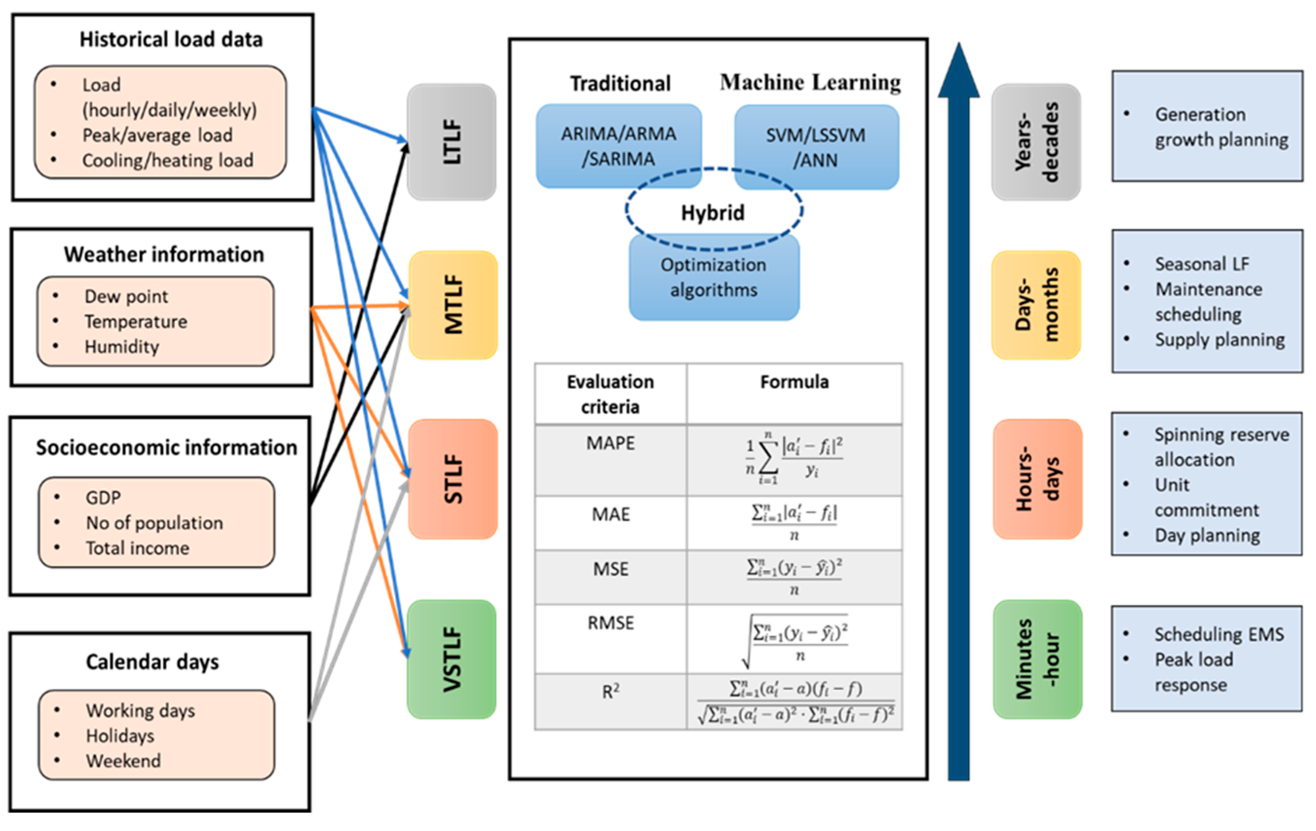
Based on the literature, electricity load forecasting has a different classification of forecasting depending on the time spans, such as very short-term load forecasting (VSTLF), short-term load forecasting (STLF), medium-term load forecasting (MTLF), and long-term load forecasting (LTLF) [6]. VSTLF is known for providing load projections in time intervals of between a few minutes to one or several hours into the future while training the prediction model utilizing historical energy loads measured on the same day [7]. It plays a significant role in scheduling building energy management system (BEMS) operations associated with the energy storage system (ESS), RE, and peak load response [8]. The STLF covers a time frame of hours to days. It plays a pivotal role in power companies’ daily operations by leveraging historical data to predict future electricity demand. This crucial information empowers companies to make informed decisions across various critical areas such as spinning reserve control, optimal unit commitment, scheduling preventive maintenance and evaluation of business contracts between companies [9]. The MTLF encompassing horizons of a few days to a few months. This timeframe proves valuable for anticipating seasonal variations in demand, such as winter or summer. Additionally, the MTLF informs critical decisions related fuel purchase, maintenance, and utility assessments [10]. The LTLF, extending beyond one year and reaching out to two decades, serves as a cornerstone for strategic planning in the power sector. It underpins crucial decisions regarding the construction of new generation capacity, shaping the very landscape of power supply and delivery systems [11].
Thus, to further recover the significant elements of the research contribution in sustaining the power market, the prior art of the literature is intensively written in the next section. Meanwhile the main contribution of the paper is as followings:
- Regarding the Malaysia geographic and environment, the correlation between weather variables and the load consumption that influences the forecasting process is analyzed using Pearson’s correlation coefficient method where the findings will influence the direction of the next generation research.
- A novel Improved Bacterial Foraging Optimization Algorithm (IBFOA) is proposed to optimize the important parameters of the LSSVM model and enhance the forecasting accuracy of the actual electricity load demand in reflecting the sustainable power market in Malaysia.
- A full support validation accuracy measures are incorporated into the proposed model to evaluate performance of the IBFOA while giving such accurate load profile demand for the power network sustainability in Malaysia.
The remainder of this paper is organized as follows. Section 2 presents the previous related work and literature gap analysis. Section 3 describes the methodology used in this study. Section 4 discussed the analysis result. Finally, Section 5 gives the conclusions of the study and future recommendations.
2. Review of Related Work
In regard to STLF, it is an inherently challenging task due to non-linearity, non-stationarity, noise, and multiple seasonality in electricity load time series. These complexities arise from diverse electrical loads influenced by weather, calendar factors, diversity of user behaviour and penetration of renewable energy solutions [12]. Due to their direct influence on the daily electricity dispatching that powers both residents’ lives and social production activities, STLF and VSTLF have emerged as the central research domains within the field of power load forecasting [13]. Additionally, STLF plays a critical role in guaranteeing the reliability of power systems, particularly during periods of scarcity or outage. Consequently, the development of accurate STLF methodologies is essential for effective energy system planning, which in turn contributes to the improvement of the country’s economic growth [14]. Hence, STLF becomes the topic of this study. Moreover, accurately predicting electricity load necessitates careful consideration of diverse influencing factors, as demonstrated from the strong correlations observed between load demand and factors such as historical load data, calendar days, and weather patterns. In this context, STLF can be characterized as a dynamic, non-linear input and output mapping function that incorporates not only historical values but also a multitude of exogenous factors, such as weather conditions [15]. For this purpose, correlation analysis plays a pivotal role in analysing the relationship between different factors and estimating their interdependencies. Pearson’s correlation coefficient (PCC) analysis is a widely used and well-established method for this purpose [16,17]. Substantial research has employed PCC analysis to investigate the interdependency between electrical load and weather variables in load forecasting, as evidenced by studies such as [18,19,20]. The selection of appropriate input variables can significantly expedite model development and enhance its forecasting accuracy [21].
Over the past few decades, the research for accurate electricity load forecasting has spurred the development of diverse methodologies, encompassing traditional statistical, machine learning algorithms, and hybrid approaches. Machine learning (ML) is a core type of artificial intelligence (AI) consisting of a group of techniques that aim to learn from data, such as artificial neural network (ANN), support vector machine (SVM), and deep learning. These types of AI techniques include methods for detecting patterns in data automatically, using these patterns to predict the future, and performing alternative ways of decision-making in an uncertain problem [22]. ANN represent intelligent algorithms inspired by the human brain’s learning mechanisms. This model has proven to be an effective tool for energy consumption forecasting due to their inherent ability to learn complex non-linear relationships from data. However, a stable result cannot be obtained due to historical dependence and overfitting of ANN when dealing with time series problems [23]. ANN have a few disadvantages, including slow convergence speed, local minima issues and disparities in structure selection. These limitations have led to the frequent substitution of ANN with the SVM [24].
On the other hand, SVM is based on the structural risk minimization principle rather than the empirical risk minimization principle and has fewer parameters to tune, thus reducing the chances of encountering problems like overlearning and local minima [25]. Different forecasting methods possess inherent strengths and weaknesses, limiting any individual method’s ability to achieve consistently exceptional performance across diverse scenarios. Motivated by the need to surpass the limitations of established forecasting methodologies, the research in electricity load forecasting models has witnessed a rising trend toward hybrid models. These models integrate popular techniques with modern evolutionary algorithms and expert systems, striving to achieve high prediction accuracy and retain interpretability simultaneously [31].
Different ANN architectures such as back-propagation (BP) neural networks [27,28], multiple layers perceptron (MLP) neural networks [29,30], recurrent neural networks [31,32], and convolutional neural networks [33] has been integrated with other AI algorithms to minimize the error value and improve the accuracy of the forecasting. Author [15] proposed a neural network based on a new modified harmony search technique for STLF. The innovative approach empowers the network to effectively capture the underlying input-output mapping function governing the forecasting process, ultimately leading to enhanced STLF accuracy. Author [34] presents the hybrid model of ANN with a Gravitational Search Algorithm (GSA) and Cuckoo Optimization Algorithm (COA) to predict monthly electricity demand of a city in Vietnam. The simulation results indicate that ANN-COA outperforms both a standalone ANN and ANN-GSA in fitting historical load data, achieving the lowest error value. Author [35] proposed coupling of Long Short Term Memory (LSTM) with sequential pattern mining (SPM) algorithm for STLF in a microgrid energy management system. An SPM algorithm is used for pattern extracting between load and meteorological data, which improves the performance of LSTM in determining the accurate future load amount with the specified relevant pattern. The implementation of forecasting based on optimization models employing Particle Swarm Optimization and Grey Wolf Optimization has enhanced the load forecasting accuracy of ML models in prime energy-consuming sectors in Iran [36]. These hybrid models, evaluated on diverse datasets exhibiting varying characteristics (type, linearity, and non-linearity), consistently outperformed standalone ML models across the forecast period up to 2040. The finding underscores the robustness of such hybrid approaches in handling small datasets with differing complexities, thereby suggesting potential for wider application in energy demand forecasting.
A regional hybrid STLF by utilizing the SVM with grasshopper optimization algorithm (GOA) techniques is proposed in [37], considering the influence factors of climatic requirements in India. Other than temperature, load, and day type, the relative humidity is incorporated in the STLF model via a similar day approach. The SVM method is also applied in STLF, where the author [38] proposed a fusion model of a based model with Rain Forest (RF) and LSTM associated with the data pre-processing method to improve the forecasting accuracy. Since SVM is only suitable for calculations with relatively small sample sizes, the functions of RF and LSTM are integrated to overcome the limitations of the single SVM model. Author [39] established a hybrid SVR for MTLF and LTLF and applied it to industrial electricity load. A hierarchical optimization method based on nested strategy and state transition algorithm (STA) is employed to find the optimal parameters of SVR. The proposed hybrid of SVR-STA has offered significant accuracy improvement compared to ANN, RNN, and SVR in the month and year dataset. The Improved Sparrow Search Algorithm (ISSA) is proposed in [40] to optimize the selection of SVM hyper-parameters and solve the shortcomings of the original SSA that are easily trapped in local optima. The hybrid model of SVM-ISSA is tested on China’s electricity consumption dataset from 2000 to 2019 and takes into account historical data of population and GDP as influencing factors to forecast the mid-long-term forecasting. In the same analysis, the hybrid ISSA-SVM shows superiority over single models. In contrast, the SVM model outperforms the ANN, reflecting the advantages of the SVM model in small samples and non-linear prediction problems. While SVM excels in generalization, its computational complexity remains high due to the quadratic programming involving inequality constraints. In response, Least Square Support Vector Machines (LSSVM) offer an improved solution by transforming these constraints into equalities, simplifying the optimization problem [41]. This significantly reduces the computational burden, making LSSVM a more attractive choice for applications in electricity load forecasting [21,42,43].
Through the summary of the above literature, the hybrid forecasting model consistently outperforms individual models in terms of forecasting accuracy. Furthermore, the inherent influence of randomly selected internal parameters on SVM performance necessitates the exploration of alternative optimization algorithm.
Evolutionary algorithms, inspired by natural selection, hold promise in identifying optimal parameter configurations for SVM, potentially leading to enhanced forecasting accuracy [44]. Among evolutionary algorithms, the Bacterial Foraging Optimization Algorithm (BFOA) garners significant recognition for its unique strengths. It excels in simultaneously exploring a vast search space (encompassing both global and local optima) and leveraging a multi-centre approach [45]. The recent evolution of BFOA has improved its configuration to overcome the shortcomings of standard BFOA in terms of complexity, execution time and convergence curve. The capability of BFOA has yielded promising results when applied to complex optimization challenges within the power system domain, such as load shedding [46,47], electric vehicle charging stations [48], frequency stabilization in hydropower systems [49], control of multi-machine power system [50,51], economic dispatch [52] and power distribution restoration [53]. The hybridization of BFOA with BP neural network [54], multi-layer bidirectional LSTM [55] and ANN [56] in STLF have been found in the literature, which shows excellent performance in improving the forecasting accuracy. However, this paper presents a novel approach by introducing the first application of Improved BFOA hybridized with LSSVM for electricity load forecasting.
Therefore, in this study, BFOA is selected to examine its suitability and performance when combined with LSSVM to forecast the load. Additionally, the bacteria’s constant step size and its movement during chemotaxis are modified using a sine cosine equation to improve BFOA, and the Improved BFOA (IBFOA) is proposed. Further, the IBFOA is used for LSSVM’s parameters optimization. Therefore, the hybrid model for load forecasting based on LSSVM-IBFOA is established. The hybrid of LSSVM-IBFOA is applied for STLF of electricity load in Peninsular Malaysia during the pandemic period. Consequently, the forecasting simulation illustrates the superiority of this hybrid optimization model compared with a single ML model and uses three methods: LSSVM, LSSVM-BFOA, and LSSVM-IBFOA.
Figure 1.
Summary of different horizons with their domain, inputs and outputs of load forecasting.
3. Methodology
The model configuration follows a process illustrated in Figure 2. For the data pre-processing, we considered data interpolation, Pearson correlation analysis, data division and data normalization. The historical load data and weather data were obtained from the local website to analyze the correlation between weather and load. The historical load data is divided into groups based on the five day-type in the week to ensure the forecasting accuracy. As the model forecasting, the LSSVM is used to forecast the load with the integration of IBFOA to optimize its parameters. Finally, the proposed hybrid model is evaluated with different accuracy measures to demonstrate its performance in STLF. Further details on these processes are explained in the next subsection.
3.1. Data Pre-Processing
3.1.1. Data Interpolation
To accurately reflect real-time behaviour within the load time series, missing values were addressed through interpolation. Specifically, the “Means by Nearby Points” method was employed, guided by the following equation:
Where and denote the two preceding values, and and signify the two subsequent values (). This approach effectively eliminates irregularities and yields a smoother load time series.
3.1.2. Pearson Correlation Analysis
This study investigates the influence of weather variables on electricity load. The linear regression model assesses the interdependence between variables using Equation (2). In this equation, Y represents the dependent variable (electricity load), X denotes the independent variable (weather variable), “a” is the y-intercept, and “b” is the slope of the regression line.
To further quantify the strength and direction of the linear relationship between weather variables and electricity demand, Pearson’s correlation coefficient is utilized. Higher absolute values of the correlation coefficient (closer to 1) indicate a stronger, linear relationship, while values closer to 0 suggest a weaker, linear relationship. Mathematically, Pearson’s correlation coefficient (r) is defined as Equation (3).
Where represents the number of data pairs, is the sum of the products of paired scores (p multiplied by w for each data point), is the sum of squared p, and is the sum of squared w.
3.1.3. Data Division
The historical load data in 2021 is collected according to the ratio of 60% as the training set, 20% as the validation set and 20% as the testing set. For forecasting in each day type, only the same day type should be used as historical load data for training, validation, and testing. The details of the dataset for each day-type are provided in Table 2.
3.1.4. Data Normalization
Data standardization is essential to ensure comparability between indicators with potentially diverse numerical ranges. This process normalizes the data by scaling it to a specific, narrower interval. In this study, a uniform mapping to the range [-1, 1] is employed. Standardization offers several benefits: it accelerates model convergence and improves accuracy while also mitigating the risk of gradient explosions.
Equation (4) represents the normalization method, where represents the value to be converted, is the converted result, is the maximum boundaries and is the minimum boundaries of the attribute values.
3.2. Least Square Support Vector Machine (LSSVM)
Unlike traditional SVM, LSSVM achieves dimensionality reduction by converting the original optimization problem with inequality constraints into one with equality constraints. This transformation allows LSSVM to utilize non-linear kernel functions, effectively projecting the input data into a higher-dimensional feature space. In this study, LSSVM is leveraging to construct an error compensation model that minimizes the difference between actual and forecasted energy consumption. Let’s denote the training data as D = {(x₁, y₁), (x₂, y₂), ..., (xₙ, yₙ)}, where xᵢ represents the i-th input vector and yᵢ represents the corresponding output (actual energy consumption). The LSSVM function for this model, mapped to the high-dimensional space, can be expressed as:
Where is the non-linear mapping function that projects the input vector (xᵢ) into a higher-dimensional space, is the bias term that influences the overall prediction, and is the weight vector that determines the influence of each feature in the high-dimensional space. This transformation through the non-linear mapping function allows the LSSVM to capture complex relationships between the input variables and the output, ultimately leading to a function optimization problem that can be expressed as:
This transformation is achieved through the following equality constraint:
Where is non-linear mapping of the k-th input vector (projected to high-dimensional space) while is a slack variable. To solve the LSSVM function optimization problem, a technique called Lagrangian transformation is employed. This method introduces Lagrange multipliers () to convert the equality constraints (Equation (7)) into an unconstrained Lagrangian function (L), defined as in Equation (8):
By applying the Karush-Kuhn-Tucker (KKT) conditions as in Equation (9), the Lagrangian function is minimized to obtain the optimal values of the ω, b, , and . This optimization process ultimately leads to the LSSVM model for error compensation in forecasting.
Equation (10) is obtained after a thorough calculation as follows:
Due to the high dimensionality of the feature space after the non-linear mapping , directly working with it can be computationally expensive. To address this, LSSVM utilizes the kernel trick. This technique leverages a kernel function that operates on the original input space (x) to compute the inner product in the high-dimensional space. The Mercer condition ensures that such a kernel function exists. Mathematically, this relationship is expressed as in Equation (11) and the final regression function of LSSVM is obtained in Equation (12).
Within the LSSVM framework for this study, the Radial Basis Function (RBF) kernel is chosen due to its well-established generalization ability and wide convergence domain. The RBF kernel function is defined as Equation (13):
Where σ (sigma) represents the width of the kernel function. Optimizing the parameters of the RBF kernel, particularly sigma (σ) and gamma (γ), is crucial for achieving optimal performance in the LSSVM model. These parameters significantly influence the model’s ability to learn from the training data and generalize well to unseen data [59]. Therefore, after obtaining the ideal of these two values, the next stage is to optimize them using IBFOA. The structure of the LSSVM model can be visualized as depicted in Figure 3. In this structure, the final output is a linear combination of the values from intermediate nodes. Notably, each intermediate node corresponds to a support vector within the LSSVM model [60].
3.3. Bacterial Foraging Optimization Algorithm
The Bacterial Foraging Optimization Algorithm (BFOA) is a population-based stochastic optimization technique inspired by the foraging behaviour of Escherichia coli (E. coli) bacteria.
Assume that the population of bacteria has S numbers, and that the present chemotactic, reproductive, and elimination-dispersal steps are represented by t, r and e respectively. At the t-th chemotactic step, r-th reproduction, and e-th elimination dispersal, the n-th bacterium’s location in the D-dimensional search space can be represented as follows:
The prominent processes take place in BFOA consisting of chemotaxis, swarming, reproduction, and elimination-dispersal are described briefly below:
- Chemotaxis: It is a process by which bacteria navigate their environment in response to chemical gradients. This behavior allows them to locate favorable conditions, such as nutrient sources. Bacteria achieve chemotaxis through a series of short runs (swims) and tumbles. Flagellar rotation determines their movement: swimming in a defined direction or tumbling to explore new areas. A unit-length random direction vector as described in Equation (15) representing a tumble for the n-th bacterium at the t-th chemotactic step, r-th reproductive step, and e-th elimination dispersal step. This vector describes the direction change after a tumble.
Where represents the n-th bacterium at the t-th chemotactic step, r-th reproductive and e-th elimination dispersal step. is the size of the step taken in the random direction specified by the tumble (the run length unit) and denotes a random direction vector that describes the movement direction of the n-th bacterium.
- Swarming: Swarming is a collective behavior in bacteria that promotes their movement towards areas with higher nutrient concentrations. This phenomenon is modeled by introducing an additional cost function term (Jcc) that influences the overall cost function (J) experienced by each bacterium. The swarming cost (Jcc) considers both the local bacterial density and the distance between individual bacteria. The mathematical representation for swarming process is expressed by Equation (17):
The coefficients associated (, , and ) influence the relative importance of swarming compared to the original cost function (J). These coefficients need to be carefully chosen or tuned to achieve optimal performance in the BFOA.
- Reproduction: Reproduction step happens after following a predefined number of chemotactic steps (Nc). This step promotes the propagation of “fitter” bacteria within the population. Bacteria with higher health values, typically determined by a fitness function have a greater chance of reproducing. Conversely, bacteria with lower health values will be eliminated. This mechanism ensures a constant population size while favoring individuals with better foraging abilities. The health value of the bacterium obtained as below:
- Elimination-dispersal: Elimination-dispersal simulates the dynamic nature of the bacterial environment, where local events can drastically affect bacterial populations. This process can either eliminate all bacteria in a local region or disperse them to new locations, potentially disrupting chemotaxis progress but also aiding in exploration by placing bacteria near potential food sources.
3.4. Proposed Improved Bacterial Foraging Optimization Algorithm
Like many other metaheuristic algorithms, the BFOA exhibits certain limitations, including high computational cost, inherent complexity, and susceptibility to getting trapped in local optima [45]. These shortcomings necessitate further research efforts to enhance the performance of BFOA and address these deficiencies. The improvement of BFOA in the existing literature mainly focuses on the chemotaxis of bacteria, as shown in [61,62,63]. Chemotaxis, the core operation of the BFOA, relies heavily on the “chemotaxis step length” parameter C(i) for effective exploration. However, the classical BFOA employs a fixed value for C(i), leading to potential drawbacks. A large constant step size might hinder bacteria from reaching distant nutrient sources, while a small value could significantly slow their movement towards nearby nutrients [64].
This study introduces an Improved Bacterial Foraging Optimization Algorithm (IBFOA) that modifies the chemotaxis operation using the Sine Cosine Algorithm (SCA) for inspiration. The key improvement lies in adapting the constant step size (C(i)) of bacteria during chemotaxis. The standard BFOA employs a fixed step size for bacterial movement during chemotaxis. The IBFOA proposes an adaptive step size defined by Equation (19):
Where a is a defined constant, and t is a count of the chemotaxis. This adaptation introduces a gradual increase in the step size as the chemotaxis process progresses. Additionally, the IBFOA incorporates a mechanism inspired by the SCA to generate random movement directions for the bacteria during chemotaxis. Equation (20) adopted from SCA generates a random direction vector for each bacterium’s movement:
Where and are the current position of the n-th bacterium and the best solution so far at the t-th chemotactic step, r-th reproduction, and e-th elimination dispersal in the d-th dimension, respectively. Variables of , and are a random number in between 0 and 2, and | | indicates the absolute value similar to SCA. The position of the n-th bacterium after a tumble is given by Equation (21):
If the bacterium encounters a higher nutrient concentration after a tumble (Equation (22)), it continues swimming in the same direction for a predefined number of swim lengths as long as the concentration increases. Conversely, if the concentration decreases, the bacterium performs another tumble to explore a new direction (Equations (19) and (20)). The remainder of the IBFOA follows the standard BFOA process, including reproduction and elimination-dispersal. This improved algorithm aims to achieve better exploration and exploitation capabilities compared to the original BFOA.
3.5. Forecasting Process by Hybrid LSSVM-IBFOA
Figure 4 illustrates the formation of a hybrid model of LSSVM-IBFOA where IBFOA will optimize the parameters of LSSVM to achieve accurate forecasting. The data pre-processing is performed through data separation and normalization of the load profile in Peninsular Malaysia. The LSSVM and IBFOA are merged to perform as a hybrid model and are simulated in MATLAB and will be built separately according to day type for better forecasting performance. The optimization process is initiated with random positions for each bacterium in the predefined dimensions, which represent the LSSVM parameters. The optimized LSSVM parameters are used to train the LSSVM. The trained model is tested on unseen data. The objective function, MAPE, is observed. The modification of IBFOA parameters is performed to optimize the LSSVM parameters, which in turn produces an accurate forecast or lowest MAPE. Table 3 provides the formation step of hybrid LSSVM-IBFOA accordingly.
3.6. Evaluation Metrics
Evaluating the accuracy of the forecasting model is crucial for assessing the effectiveness of the proposed methods. This section discusses the key performance criteria used in this study. The mean absolute error (MAE) and mean absolute percentage error (MAPE) are the most important static metrics used by researchers [65]. In the simulation, MAPE is utilized as an objective function of LSSVM-IBFOA (fitness function value). It is widely adopted performance measure in the electric power industry due to its simplicity and ease of interpretation [66]. The MAPE value was classified into four forecasting capabilities, as provided in Table 4 [67].
A thorough assessment of the model’s performance requires employing a diverse set of accuracy measures. This section details the metrics used in this study along with their interpretations. These accuracy measures include MAE, MSE, RMSE, R2, NRMSE and NMSE, which are obtained by equations in Table 5, where p is the total number of forecasting data, is the actual value, is the forecasted value and is the average value of forecasted value [68]. The best state to evaluate the accuracy of forecasting results using such measures is the maximum value for R2 and the minimum values for forecasting error measures [69].
4. Results and Discussion
4.1. Correlation Analysis
In this analysis, some of the weather variables considered include relative humidity, dew point and temperature. Relative humidity signifies the ratio of water vapor present in the air compared to the maximum amount it can hold at that temperature, expressed as a percentage. Higher humidity during warmer months amplifies the sensation of heat compared to the actual temperature [16]. These weather variables are often included together due to their inherent interdependencies.
Table 6 presents the correlation coefficient between the load consumption and the model inputs. Notably, the previous day’s load exhibits a strong positive correlation with the current day’s load, indicating a significant influence on the forecasted load. The relative humidity and temperature show a moderate correlation, while the dew point shows weak and no correlation with load because the correlation coefficients are less than ±0.6, as mentioned in Table 1. Thus, the simulation model only considered the input from previous load with strong correlation whereas weather variables are neglected.
4.2. Case Study
In this study, the electricity load of Peninsular Malaysia during the COVID-19 pandemic is used as a case study for evaluating the efficiency of the proposed model in disrupted situations. The hourly electricity load demand in megawatts (MW) in 2021 is used as raw input data. Figure 5 depicts the monthly average electricity load demand in 24 hours, illustrating the characteristics of the electricity load pattern. During the year of pandemic (2020 and 2021), the electricity load fluctuated and did not follow the trend of the pre-pandemic (2019). For instance, in March 2020, the electricity load dropped by 23.54% compared to the same month in 2019. This is due to the enforcement of the initial MCO (MCO 1.0) on 18 March which closed non-essential business operations and restricted human daily activities to control the spread of the virus. The MCO 2.0 was enforced in the early months of 2021 but failed to achieve a significant reduction in COVID-19 cases as it was only enforced in certain states. Therefore, the full nationwide lockdown (MCO 3.0) was implemented in June 2021 due to the rising of COVID-19 cases. Consequently, the average electricity consumption in June 2021 was 1109 MW lower than the average consumption for the same month in 2019, which represents a reduction of 7.69%. From October 2021, a recovery in the load demand can be seen with the further easing of some restrictions and allowing some activities to continue.
The COVID-19 pandemic is considered as the crisis event due to the unprecedented measures implemented and the demand pattern during the pandemic is expected to be different than previous periods. Thus, electricity demand needs to be forecasted considering the fluctuated demand pattern. Although the impact of pandemic is obvious, accurate forecasting remains essential for effective market operations and system planning [73]. Therefore, in this paper, the load demand from June until October 2021 is taken as the case study to observe the ability of the LSSVM based model to forecast the future load pattern based on past load behaviour during pandemic.
4.3. Load Forecasting Results
The following section presents an analysis of the performance of LSSVM in conjunction with BFOA and IBFOA based on different evaluation criteria, as listed in Table 5. In this paper, three models, namely LSSVM, LSSVM-BFOA, and LSSVM-IBFOA, were utilized to forecast the daily electricity load in Peninsular Malaysia for short-term analysis. The LSSVM model was trained using the RBF as the kernel function, while IBFOA was employed to optimize the parameters of LSSVM. The input data from historical load data was separated into 5-day types in a week as follows:
Day-type: Monday
Day-type: Tuesday, Wednesday, Thursday (Tuesday-Thursday)
Day-type: Friday
Day-type: Saturday
Day-type: Sunday
Forecasts for Tuesday, Wednesday, and Thursday of each month were aligned due to their similar load curve patterns.
Figure 6a–e compare the forecasted load demand from LSSVM, LSSVM-BFOA, and LSSVM-IBFOA models with the real load demand in Peninsular Malaysia for each day type in the testing dataset for four weeks (28 October-21 November 2021). The load demand fluctuates depending on the time of day, starting from modest levels in the early morning, rising as the day progresses, and slowing down as night approaches. Also, the load demand curve on weekends, especially Sundays, appears different compared to the weekday (Monday to Friday) load demand curve. The Sunday load profile exhibits a distinct pattern with a higher starting demand from 12:00 AM, a gradual decrease until 8:00 AM, and a subsequent rise until 7:00 PM. The data separation highlights the importance of incorporating predefined day types in the forecasting model.
The simulations show that the forecasted load curve by the three models on Monday has the most similar pattern to the actual load curve as depicted in Figure 6a. An analysis of the average absolute differences reveals a clear advantage for the LSSVM-IBFOA model in consistently following the actual load profile across all four days. Particularly, LSSVM-IBFOA, LSSVM-BFOA and LSSVM achieved the average absolute difference across the four days with the value of 1.42%, 1.95% and 3.99% respectively. However, there is a gap between the forecasted load curve and the actual load curve at peak times of the day, especially on Friday and Tuesday-Thursday, which has the largest forecasting error value. The significant discrepancy between the forecasted and actual load, with all forecasting models underestimating demand is observed on Friday load profile as shows in Figure 6c. Examining the average absolute differences across the four days’ reveals that all models exhibited underestimation with the highest on the first day, with LSSVM (highest - 10.27%) showing the greatest deviation, followed by LSSVM-BFOA (9.43%) and LSSVM-IBFOA (lowest - 8.95%). For weekends load profile, while all forecasting models exhibited some level of underestimation, particularly during peak hours, the deviations were generally lower compared to other weekdays (Friday and Tuesday-Thursday).
Table 7 provides a detailed comparison of error metrics for the forecasting models evaluated on the 2021 testing dataset, categorized by day-type (Monday through Sunday). The testing dataset show consistent reductions in error metrics across all day-types for LSSVM-IBFOA compared to both LSSVM and LSSVM-BFOA. Notably, across the five day-type (Monday, Tuesday-Thursday, Friday, Saturday and Sunday), MAPE reductions obtained are 64.21%, 40.86%, 13.54%, 16.00% and 7.24% respectively, signifying significant improvements. Similarly, reductions were observed for MAE (62.45%, 42.70%, 14.35%, 17.35% and 8.51%), RMSE and NRMSE (60.52%, 43.91%, 14.03%, 14.98% and 17.30%), and MSE (84.41%, 68.54%, 26.10%, 27.72%, 31.62%). These reductions highlight the improved ability of LSSVM-IBFOA to minimize forecasting errors compared to the baseline LSSVM model.
Similarly, LSSVM-IBFOA has outperforms LSSVM-BFOA with minimal reductions of MAPE (26.89%, 4.85%, 4.37%, 2.80%, and 0.19%), MAE (27.33%, 9.05%, 4.36%, 3.27% and 2.00%), RMSE and NRMSE (25.10%, 3.99%, 3.42%, 0.17% and 10.02%), and MSE (43.91%, 7.83%, 6.72%, 0.35%, 19.03%). In terms of R², the LSSVM-IBFOA achieves the highest value (0.9880) on Monday and the lowest (0.8901) on Friday. Conversely, LSSVM-BFOA and LSSVM exhibit a wider range of R2, with Mondays reaching 0.9824 and 0.9593, and Sundays dropping to 0.7405 and 0.4719, respectively. This observation suggests that LSSVM-IBFOA maintains a consistently high R² across weekdays, indicating a strong correlation between predicted and actual values. While both LSSVM-IBFOA and LSSVM-BFOA demonstrate effectiveness compared to LSSVM, LSSVM-IBFOA outperforms LSSVM-BFOA on average. These observations on the testing dataset highlight the effectiveness of LSSVM-IBFOA in achieving superior overall forecasting accuracy. The optimization process introduced by the IBFOA algorithm empowers LSSVM to deliver forecasts with consistently lower errors and a strong positive correlation with actual values across different weekdays and weekends. These reductions highlight the effectiveness of LSSVM-IBFOA’s optimization process in generalizing well to unseen data compared to LSSVM-BFOA.
Figure 7 summarizes the visualization results of accuracy measures from three models focusing on the important results. The error values of the models obtained demonstrate that Monday had the best performance with high accuracy compared to other day types. From the above analysis, the electricity load forecasting result of using IBFOA to optimize the LSSVM model demonstrated better results than standard BFOA and stand-alone LSSVM. Thus, the effectiveness of the proposed hybrid model is proved.
4.4. Algorithm Performance
Figure 8a–e depicts the convergence curve for IBFOA and BFOA, which is represented by the fitness value (MAPE) over the iteration. Table 8 represents the convergence time obtained for each day type, which shows that the IBFOA has a shorter convergence time than the BFOA. The IBFOA improves the convergence speed and accuracy of BFOA. SCA has a high speed due to its simple structure. At the same time, the reproduction and elimination dispersal processes give BFOA an advantage in accelerating the exploitation phase and preventing the algorithm from falling into local optima. Therefore, the IBFOA has better performance in terms of convergence speed, accuracy, and local optima avoidance by synergizing the strengths of both algorithms. From the analysis, considering five-day types in a week, the IBFOA converges at 398th, 31st, 92nd, 231th, and 532th iterations, respectively. In contrast, the BFOA converges at the 477th, 111th, 143rd, 301st and 682nd iterations, respectively.
5. Conclusions
Understanding future electricity demand patterns constitutes a critical factor in ensuring the stability and security of energy systems especially in Malaysia power market. This information proves invaluable for government authorities as they make strategic decisions and plan a power system for the sustainable growth of a country. To forecast the electric load accurately, in this paper, a hybrid method based on LSSVM optimized by IBFOA (LSSVM-IBFOA) for daily electricity load forecasting is proposed. The Pearson Correlation is utilized to analyze the correlation of present load with past load and weather. The past weather data incorporating temperature, humidity, and dew point are negligible since they show no until moderate correlation with the load. Thus, the historical load with a strong correlation is taken as the input to the LSSVM. For parameter optimization of LSSVM, an IBFOA is proposed to overcome the shortcomings of fixed constant value in chemotaxis from the original BFOA, thus improving the convergence accuracy and optimization performance of BFOA. The proposed approach, LSSVM-IBFOA, is used to forecast the daily electricity load in peninsular Malaysia during the pandemic based on the historical load data from June 2021 until October 2021, considering the five-day types in a week. The simulation result demonstrates that the hybrid of LSSVM-IBFOA outperforms the LSSVM and LSSM-BFOA with the lowest value of MAPE, MAE, RMSE, MSE and NRMSE as well as the biggest R2 for all day types. On average, the values obtained from the day type were 4.1615%, 617.6613, 730.0336, 646979.9275, 0.0498 and 0.9464 respectively. The recommendations for future directions are included but not limited to:
- a)
- Increasing the size of the dataset to one year or more to see the performance of LSSVM in training the data,
- b)
- Application for LSSVM-IBFOA for load forecasting on a smaller load aggregation such as residential or building,
- c)
- Test different combinations of feature/input sets which represent the primary consumption,
- d)
- Hybridizing the LSSVM model with other newly nature-inspired algorithms, data decomposition techniques, and feature selection methods to improve ML forecasting performance.
Author Contributions
F.A.Z.; methodology, writing-original draft preparation, software, M.F.S.; writing—review and editing, supervision, I.A.W.A.R.; software, methodology, validation, M.L.O.; writing—review and editing, H.M.; visualization and investigation. All authors have read and agreed to the published version of the manuscript.
Funding
This research received no external funding.
Data Availability Statement
The data presented in this study are available on request from the corresponding author due to restrictions privacy.
Acknowledgments
The authors would like to thank Universiti Teknikal Malaysia Melaka (UTeM) for all the support given.
Conflicts of Interest
The authors declare no conflicts of interest. The funders had no role in the design of the study; in the collection, analyses, or interpretation of data; in the writing of the manuscript; or in the decision to publish the results.
References
- Z. Zulkifli, “Malaysia Country Report,” 17 th AsiaConstruct Conf., no. 72, pp. 170–190, 2021.
- IRENA, Malaysia energy transition outlook. International Renewable Energy Agency, Abu Dhabi, 2023. [Online]. Available: www.irena.org.
- L. Aswanuwath, W. Pannakkong, J. Buddhakulsomsiri, and J. Karnjana, “An Improved Hybrid Approach for Daily Electricity Peak Demand Forecasting during Disrupted Situations : A Case Study of COVID-19 Impact in Thailand,” Energies, vol. 17, no. 78, 2023.
- F. Abd. Razak, M. Shitan, A. H. Hashim, and I. Z. Abidin, “Load Forecasting Using Time Series Models,” J. Kejuruter., vol. 21, no. 1, pp. 53–62, 2009. [CrossRef]
- L. Hock-Eam and Y. Chee-Yin, “How accurate is TNB’s electricity demand forecast?,” Malaysian J. Math. Sci., vol. 10, pp. 79–90, 2016.
- A. A. Mir, M. Alghassab, K. Ullah, Z. A. Khan, Y. Lu, and M. Imran, “A review of electricity demand forecasting in low and middle income countries: The demand determinants and horizons,” Sustain., vol. 12, no. 15, 2020. [CrossRef]
- P. Koukaras, N. Bezas, P. Gkaidatzis, D. Ioannidis, D. Tzovaras, and C. Tjortjis, “Introducing a novel approach in one-step ahead energy load forecasting,” Sustain. Comput. Informatics Syst., vol. 32, no. August, p. 100616, 2021. [CrossRef]
- J. Moon, S. Jung, J. Rew, S. Rho, and E. Hwang, “Combination of short-term load forecasting models based on a stacking ensemble approach,” Energy Build., vol. 216, p. 109921, 2020. [CrossRef]
- B. U. Islam, M. Rasheed, and S. F. Ahmed, “Review of Short-Term Load Forecasting for Smart Grids Using Deep Neural Networks and Metaheuristic Methods,” Math. Probl. Eng., vol. 2022, 2022. [CrossRef]
- I. K. Nti, M. Teimeh, O. Nyarko-Boateng, and A. F. Adekoya, “Electricity load forecasting: a systematic review,” J. Electr. Syst. Inf. Technol., vol. 7, no. 1, Dec. 2020. [CrossRef]
- M. A. Hammad, B. Jereb, B. Rosi, and D. Dragan, “Methods and Models for Electric Load Forecasting: A Comprehensive Review,” Logist. Sustain. Transp., vol. 11, no. 1, pp. 51–76, 2020. [CrossRef]
- S. Pelekis et al., “A comparative assessment of deep learning models for day-ahead load forecasting: Investigating key accuracy drivers,” Sustain. Energy, Grids Networks, vol. 36, p. 101171, 2023. [CrossRef]
- H. Luo, H. Zhang, and J. Wang, “Ensemble power load forecasting based on competitive-inhibition selection strategy and deep learning,” Sustain. Energy Technol. Assessments, vol. 51, no. June 2021, p. 101940, 2022. [CrossRef]
- C. Tarmanini, N. Sarma, C. Gezegin, and O. Ozgonenel, “Short term load forecasting based on ARIMA and ANN approaches,” Energy Reports, vol. 9, pp. 550–557, 2023. [CrossRef]
- N. Amjady and F. Keynia, “A new neural network approach to short term load forecasting of electrical power systems,” Energies, vol. 4, no. 3, pp. 488–503, 2011. [CrossRef]
- M. Jawad et al., “Machine Learning Based Cost Effective Electricity Load Forecasting Model Using Correlated Meteorological Parameters,” IEEE Access, vol. 8, pp. 146847–146864, 2020. [CrossRef]
- G.-T. L. F. of the G. E. S. Stamatellos and T. Stamatelos, “Short-Term Load Forecasting of the Greek Electricity System,” Appl. Sci., vol. 13, no. 4, 2023. [CrossRef]
- T. Ahmed, D. H. Vu, K. M. Muttaqi, and A. P. Agalgaonkar, “Load forecasting under changing climatic conditions for the city of Sydney, Australia,” Energy, vol. 142, pp. 911–919, 2018. [CrossRef]
- T. Ahmad, H. Chen, J. Shair, and C. Xu, “Deployment of data-mining short and medium-term horizon cooling load forecasting models for building energy optimization and management,” Int. J. Refrig., vol. 98, pp. 399–409, 2019. [CrossRef]
- Y. Wang et al., “Short-term load forecasting for industrial customers based on TCN-LightGBM,” IEEE Trans. Power Syst., vol. 36, no. 3, pp. 1984–1997, 2021. [CrossRef]
- A. Yang, W. Li, and X. Yang, “Short-term electricity load forecasting based on feature selection and Least Squares Support Vector Machines,” Knowledge-Based Syst., vol. 163, pp. 159–173, Jan. 2019. [CrossRef]
- I. Antonopoulos et al., “Artificial intelligence and machine learning approaches to energy demand-side response: A systematic review,” Renewable and Sustainable Energy Reviews, vol. 130. Elsevier Ltd., Sep. 01, 2020. [CrossRef]
- Y. Dai, X. Yang, and M. Leng, “Forecasting power load: A hybrid forecasting method with intelligent data processing and optimized artificial intelligence,” Technol. Forecast. Soc. Change, vol. 182, no. July, p. 121858, 2022. [CrossRef]
- I. A. W. A. Razak, W. S. W. Abdullah, and M. F. Sulaima, “Enhanced Short-term System Marginal Price (SMP) Forecast Modelling Using a Hybrid Model Combining Least Squares Support Vector Machines and the Genetic Algorithm in Peninsula Malaysia,” Int. J. Intell. Syst. Appl. Eng., vol. 11, no. 4, pp. 289–298, 2023.
- C. Zhang, J. Zhou, C. Li, W. Fu, and T. Peng, “A compound structure of ELM based on feature selection and parameter optimization using hybrid backtracking search algorithm for wind speed forecasting,” Energy Convers. Manag., vol. 143, pp. 360–376, 2017. [CrossRef]
- S. Li et al., “Short-term electrical load forecasting using hybrid model of manta ray foraging optimization and support vector regression,” J. Clean. Prod., vol. 388, p. 135856, 2023. [CrossRef]
- Y. Yang, Y. Chen, Y. Wang, C. Li, and L. Li, “Modelling a combined method based on ANFIS and neural network improved by DE algorithm: A case study for short-term electricity demand forecasting,” Applied Soft Computing Journal, vol. 49. Elsevier Ltd., pp. 663–675, Dec. 01, 2016. [CrossRef]
- W. Aribowo, “Optimizing Feed Forward Backpropagation Neural Network Based on Teaching-Learning-Based Optimization Algorithm for Long-Term Electricity Forecasting,” Int. J. Intell. Eng. Syst., vol. 15, no. 1, pp. 11–20, 2022. [CrossRef]
- R. Liang, T. Le-Hung, and T. Nguyen-Thoi, “Energy consumption prediction of air-conditioning systems in eco-buildings using hunger games search optimization-based artificial neural network model,” J. Build. Eng., vol. 59, no. August, p. 105087, 2022. [CrossRef]
- M. Askari and F. Keynia, “Mid-term electricity load forecasting by a new composite method based on optimal learning MLP algorithm,” IET Gener. Transm. Distrib., vol. 14, no. 5, pp. 845–852, Mar. 2020. [CrossRef]
- N. Bacanin et al., “Multivariate energy forecasting via metaheuristic tuned long-short term memory and gated recurrent unit neural networks,” Inf. Sci. (Ny)., vol. 642, no. January, p. 119122, 2023. [CrossRef]
- R. Kottath and P. Singh, “Influencer buddy optimization: Algorithm and its application to electricity load and price forecasting problem,” Energy, vol. 263, Jan. 2023. [CrossRef]
- H. J. Sadaei, P. C. de Lima e Silva, F. G. Guimarães, and M. H. Lee, “Short-term load forecasting by using a combined method of convolutional neural networks and fuzzy time series,” Energy, vol. 175, pp. 365–377, 2019. [CrossRef]
- J. F. Chen, S. K. Lo, and Q. H. Do, “Forecasting monthly electricity demands: An application of neural networks trained by heuristic algorithms,” Inf., vol. 8, no. 1, 2017. [CrossRef]
- A. Jahani, K. Zare, and L. Mohammad Khanli, “Short-term load forecasting for microgrid energy management system using hybrid SPM-LSTM,” Sustain. Cities Soc., vol. 98, no. July, p. 104775, 2023. [CrossRef]
- M. Emami Javanmard and S. F. Ghaderi, “Energy demand forecasting in seven sectors by an optimization model based on machine learning algorithms,” Sustain. Cities Soc., vol. 95, no. October 2022, p. 104623, 2023. [CrossRef]
- M. Barman, N. B. Dev Choudhury, and S. Sutradhar, “A regional hybrid GOA-SVM model based on similar day approach for short-term load forecasting in Assam, India,” Energy, vol. 145, pp. 710–720, 2018. [CrossRef]
- W. Guo, L. Che, M. Shahidehpour, and X. Wan, “Machine-Learning based methods in short-term load forecasting,” Electr. J., vol. 34, no. 1, Jan. 2021. [CrossRef]
- Z. Wang, X. Zhou, J. Tian, and T. Huang, “Hierarchical parameter optimization based support vector regression for power load forecasting,” Sustain. Cities Soc., vol. 71, no. April, p. 102937, 2021. [CrossRef]
- J. Li, Y. Lei, and S. Yang, “Mid-long term load forecasting model based on support vector machine optimized by improved sparrow search algorithm,” Energy Reports, vol. 8, pp. 491–497, 2022. [CrossRef]
- L. Yang, S. Yang, S. Li, R. Zhang, F. Liu, and L. Jiao, “Coupled compressed sensing inspired sparse spatial-spectral LSSVM for hyperspectral image classification,” Knowledge-Based Syst., vol. 79, pp. 80–89, 2015. [CrossRef]
- Q. Ge et al., “Industrial Power Load Forecasting Method Based on Reinforcement Learning and PSO-LSSVM,” IEEE Trans. Cybern., vol. 52, no. 2, pp. 1112–1124, 2022. [CrossRef]
- G. Wang, X. Wang, Z. Wang, C. Ma, and Z. Song, “A VMD-CISSA-LSSVM Based Electricity Load Forecasting Model,” Mathematics, vol. 10, no. 1, 2022. [CrossRef]
- S. Zhang, N. Zhang, Z. Zhang, and Y. Chen, “Electric Power Load Forecasting Method Based on a Support Vector Machine Optimized by the Improved Seagull Optimization Algorithm,” Energies, vol. 15, no. 23, 2022. [CrossRef]
- B. Khan, K. Redae, E. Gidey, O. P. Mahela, I. B. M. Taha, and M. G. Hussien, “Optimal integration of DSTATCOM using improved bacterial search algorithm for distribution network optimization,” Alexandria Eng. J., vol. 61, no. 7, pp. 5539–5555, 2022. [CrossRef]
- H. Awad and A. Hafez, “Optimal operation of under-frequency load shedding relays by hybrid optimization of particle swarm and bacterial foraging algorithms,” Alexandria Eng. J., vol. 61, no. 1, pp. 763–774, 2022. [CrossRef]
- H. M. V. Nguyen, T. T. Phung, T. N. Le, N. A. Nguyen, Q. T. Nguyen, and P. N. Nguyen, “Using an improved Neural Network with Bacterial Foraging Optimization algorithm for Load Shedding,” Proc. 2023 Int. Conf. Syst. Sci. Eng. ICSSE 2023, pp. 281–286, 2023. [CrossRef]
- W. S. Tounsi Fokui, M. J. Saulo, and L. Ngoo, “Optimal Placement of Electric Vehicle Charging Stations in a Distribution Network with Randomly Distributed Rooftop Photovoltaic Systems,” IEEE Access, vol. 9, pp. 132397–132411, 2021. [CrossRef]
- A. Panwar, G. Sharma, I. Nasiruddin, and R. C. Bansal, “Frequency stabilization of hydro–hydro power system using hybrid bacteria foraging PSO with UPFC and HAE,” Electr. Power Syst. Res., vol. 161, pp. 74–85, 2018. [CrossRef]
- R. Kumar, S. Diwania, R. Singh, H. Ashfaq, P. Khetrapal, and S. Singh, “An intelligent Hybrid Wind–PV farm as a static compensator for overall stability and control of multimachine power system,” ISA Trans., vol. 123, pp. 286–302, 2022. [CrossRef]
- M. Zadehbagheri, T. Sutikno, M. J. Kiani, and M. Yousefi, “Designing a power system stabilizer using a hybrid algorithm by genetics and bacteria for the multi-machine power system,” Bull. Electr. Eng. Informatics, vol. 12, no. 3, pp. 1318–1331, 2023. [CrossRef]
- Y. Zhang, Y. Lv, and Y. Zhou, “Research on Economic Optimal Dispatching of Microgrid Based on an Improved Bacteria Foraging Optimization,” Biomimetics, vol. 8, no. 2, p. 150, 2023. [CrossRef]
- C. I. de A. C. Carlos Henrique Valério de Moraes, Jonas Lopes de Vilas Boas, Germano Lambert-Torres, Gilberto Capistrano Cunha de Andrade, “Intelligent Power Distribution Restoration Based on a Multi-Objective Bacterial Foraging Optimization Algorithm,” Energies, vol. 15(4), p. 1445, 2022. [CrossRef]
- Y. Han, H. Xiong, and D. Wei, “Short-term load forecasting of BP network based on bacterial foraging optimization,” IOP Conf. Ser. Mater. Sci. Eng., vol. 569, no. 5, 2019. [CrossRef]
- Z. Zhou, G. Wu, and X. Zhang, “Short-term Load Forecasting Model Based on IBFO-BILSTM,” IOP Conf. Ser. Earth Environ. Sci., vol. 440, no. 3, 2020. [CrossRef]
- Y. Zhang, L. Wu, and S. Wang, “Bacterial foraging optimization based neural network for short-term load forecasting,” J. Comput. Inf. Syst., vol. 6, no. 7, pp. 2099–2105, 2010.
- Y. Jiang et al., “Medium-long term load forecasting method considering industry correlation for power management,” Energy Reports, vol. 7, pp. 1231–1238, 2021. [CrossRef]
- X. Zhi, S. Yuexin, M. Jin, Z. Lujie, and D. Zijian, “Research on the Pearson correlation coefficient evaluation method of analog signal in the process of unit peak load regulation,” ICEMI 2017 - Proc. IEEE 13th Int. Conf. Electron. Meas. Instruments, vol. 2018-Janua, pp. 522–527, 2017. [CrossRef]
- K. Gao, X. Xu, and S. Jiao, “Prediction and visualization analysis of drilling energy consumption based on mechanism and data hybrid drive,” Energy, vol. 261, no. PA, p. 125227, 2022. [CrossRef]
- X. Yuan, C. Chen, Y. Yuan, Y. Huang, and Q. Tan, “Short-term wind power prediction based on LSSVM-GSA model,” Energy Convers. Manag., vol. 101, pp. 393–401, 2015. [CrossRef]
- Y. Zhang and Y. Lv, “Research on electrical load distribution using an improved bacterial foraging algorithm,” Front. Energy Res., vol. 11, no. February, pp. 1–12, 2023. [CrossRef]
- C. Y. Lee et al., “Hybrid algorithm based on simulated annealing and bacterial foraging optimization for mining imbalanced data,” Sensors Mater., vol. 33, no. 42, pp. 1297–1312, 2021. [CrossRef]
- A. Sharma, “Adaptive bacterial foraging optimization based task scheduling in cloud computing,” J. Green Eng., vol. 10, no. 11, pp. 10189–10202, 2020.
- S. Mohammad et al., “Sine based Bacterial Foraging Algorithm for a Dynamic Modelling of a Twin Rotor System,” Int. Conf. Control. Autom. Syst., vol. 2019-Octob, no. Iccas 2019, pp. 131–136, 2019. [CrossRef]
- N. Ahmad, Y. Ghadi, M. Adnan, and M. Ali, “Load Forecasting Techniques for Power System: Research Challenges and Survey,” IEEE Access, vol. 10, pp. 71054–71090, 2022. [CrossRef]
- T. Hong and S. Fan, “Probabilistic electric load forecasting: A tutorial review,” Int. J. Forecast., vol. 32, no. 3, pp. 914–938, 2016. [CrossRef]
- E. Vivas, H. Allende-Cid, and R. Salas, “A systematic review of statistical and machine learning methods for electrical power forecasting with reported mape score,” Entropy, vol. 22, no. 12, pp. 1–24, 2020. [CrossRef]
- C. Sekhar and R. Dahiya, “Robust framework based on hybrid deep learning approach for short term load forecasting of building electricity demand,” Energy, vol. 268, no. September 2022, p. 126660, 2023. [CrossRef]
- A. Moradzadeh, S. Zakeri, M. Shoaran, B. Mohammadi-Ivatloo, and F. Mohammadi, “Short-term load forecasting of microgrid via hybrid support vector regression and long short-term memory algorithms,” Sustain., vol. 12, no. 17, 2020. [CrossRef]
- G. F. Fan, L. Z. Zhang, M. Yu, W. C. Hong, and S. Q. Dong, “Applications of random forest in multivariable response surface for short-term load forecasting,” Int. J. Electr. Power Energy Syst., vol. 139, no. May 2021, p. 108073, 2022. [CrossRef]
- N. Tsalikidis, A. Mystakidis, C. Tjortjis, P. Koukaras, and D. Ioannidis, “Energy load forecasting: one-step ahead hybrid model utilizing ensembling,” Computing, no. 0123456789, 2023. [CrossRef]
- A. Groß, A. Lenders, F. Schwenker, D. A. Braun, and D. Fischer, “Comparison of short-term electrical load forecasting methods for different building types,” Energy Informatics, vol. 4, no. Suppl 3, 2021. [CrossRef]
- A. Kök, E. Yükseltan, M. Hekimoğlu, E. A. Aktunc, A. Yücekaya, and A. Bilge, “Forecasting Hourly Electricity Demand Under COVID-19 Restrictions,” Int. J. Energy Econ. Policy, vol. 12, no. 1, pp. 73–85, 2022. [CrossRef]
Figure 2.
Framework for electricity load forecasting.
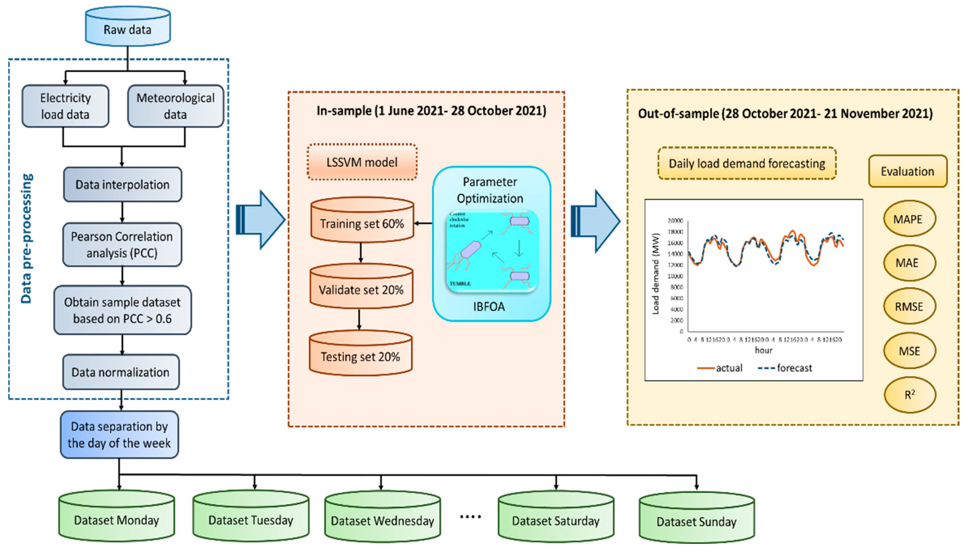
Figure 3.
Structures of LSSVM.
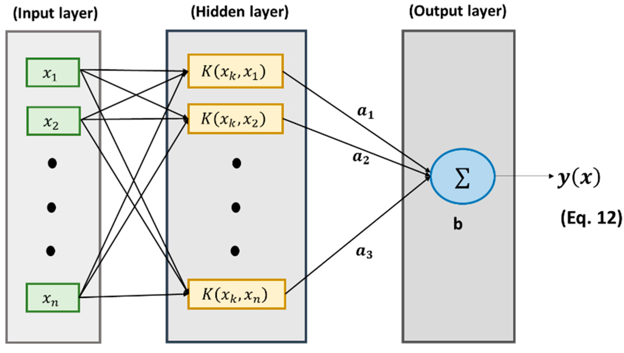
Figure 4.
The flowchart of LSSVM-IBFOA.
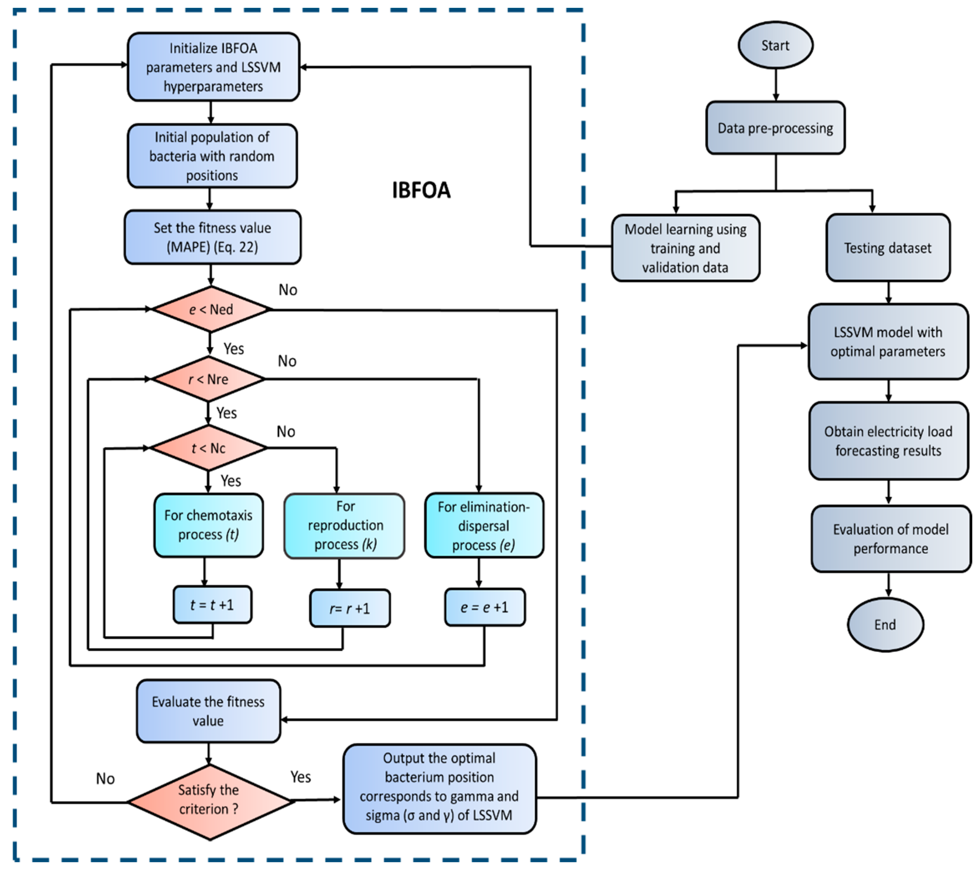
Figure 5.
Monthly average electricity load profile in 24 hours (2019-2021).
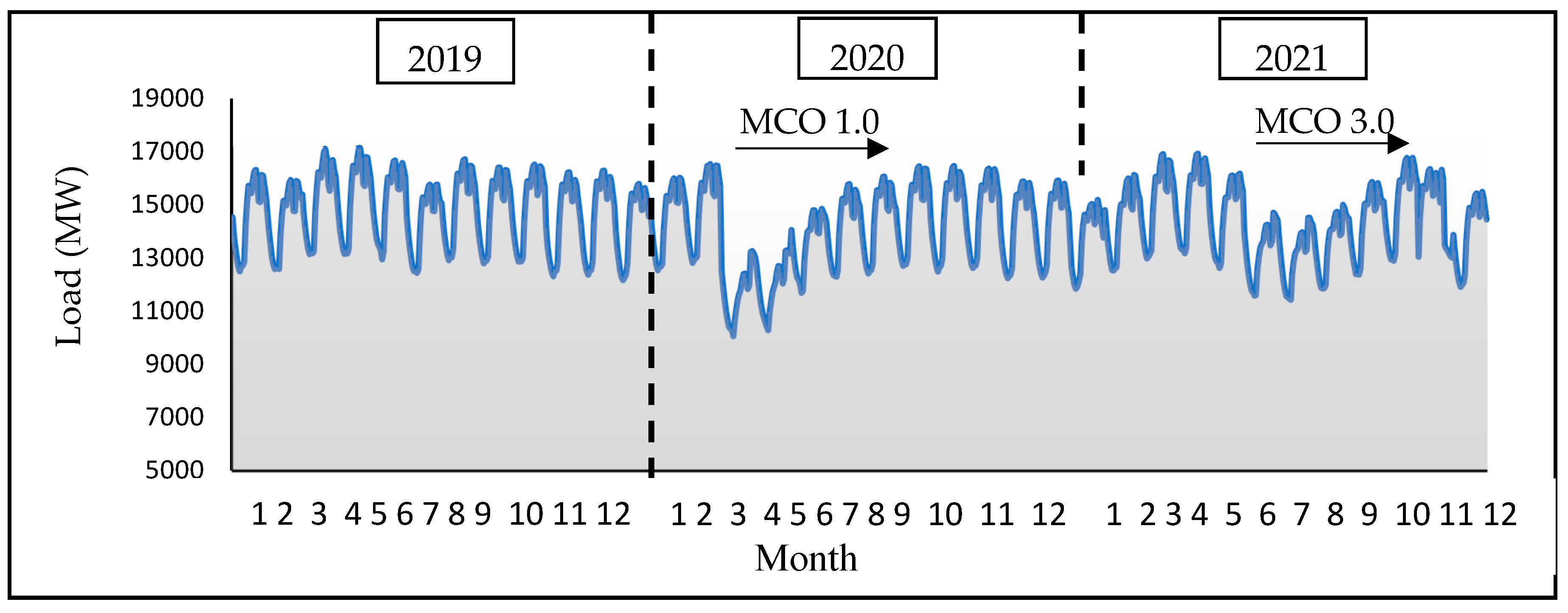
Figure 6.
Visualization of forecasting result for the LSSVM, LSSVM-BFOA, LSSVM-IBFOA for: (a) Monday; (b) Tuesday-Thursday; (c) Friday; (d) Saturday and (e) Sunday.
Figure 6.
Visualization of forecasting result for the LSSVM, LSSVM-BFOA, LSSVM-IBFOA for: (a) Monday; (b) Tuesday-Thursday; (c) Friday; (d) Saturday and (e) Sunday.
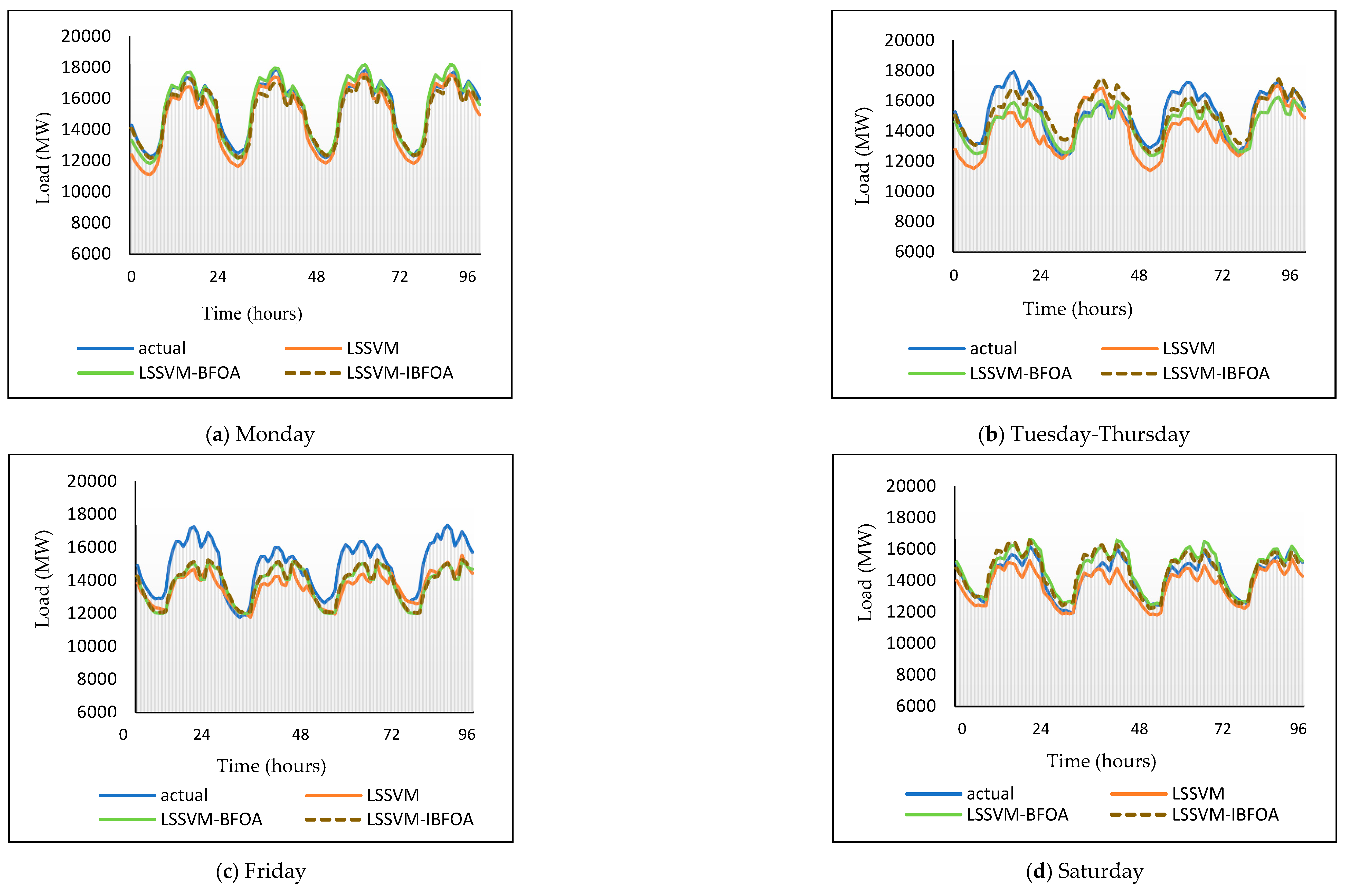
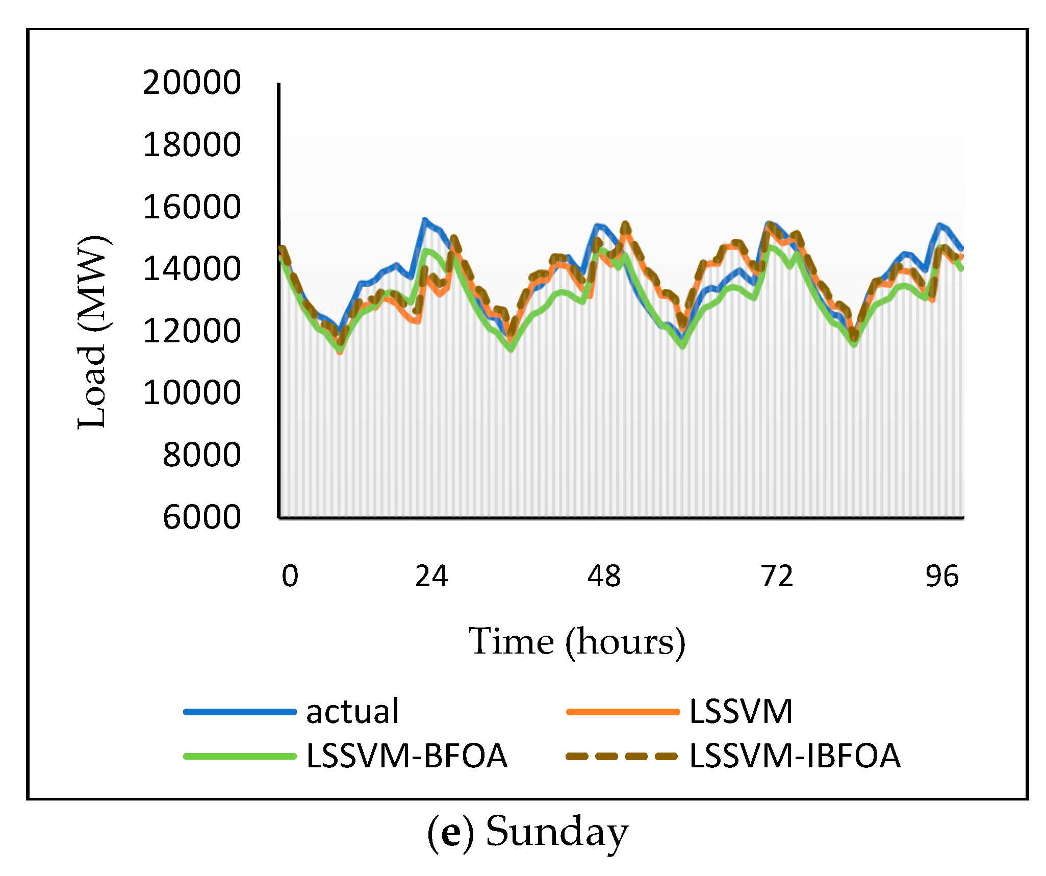
Figure 7.
Illustrations of plots for MAPE and MAE.
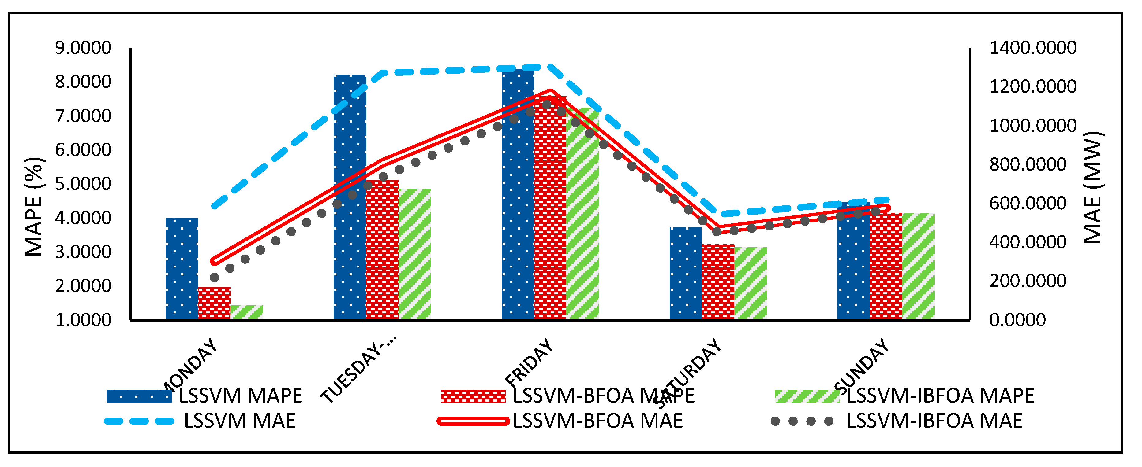
Figure 8.
Convergence curve of BFOA and IBFOA for: (a) Monday; (b) Tuesday-Thursday; (c) Friday; (d) Saturday; and (e) Sunday.
Figure 8.
Convergence curve of BFOA and IBFOA for: (a) Monday; (b) Tuesday-Thursday; (c) Friday; (d) Saturday; and (e) Sunday.
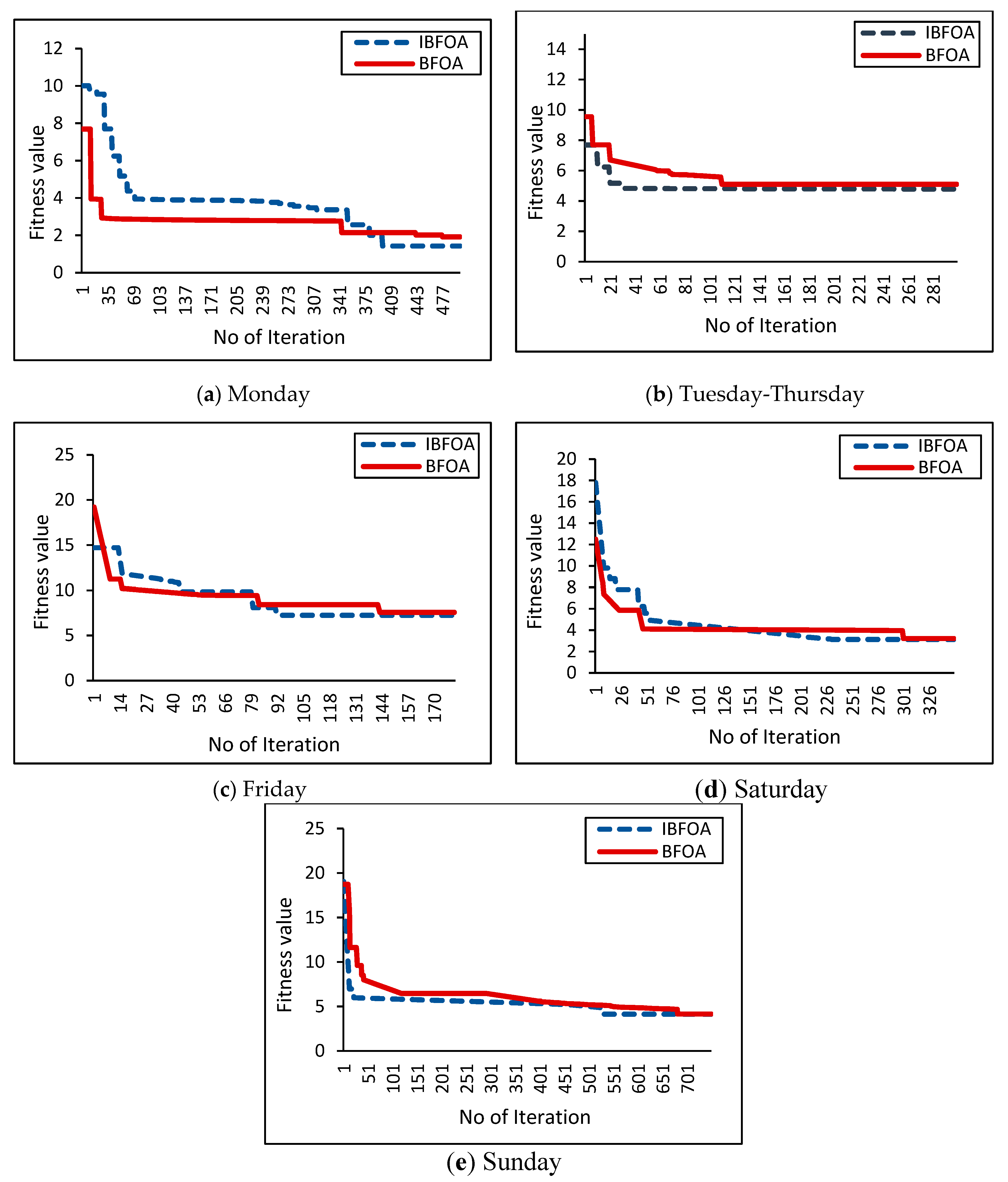

Table 1.
Descriptive condition based on the person correlation coefficient.
| Condition | Description |
|---|---|
| = +1 | linear and perfect positive correlation |
| < 1.0 | very strong linear correlation |
| < 0.8 | strong linear correlation |
| < 0.6 | moderate linear correlation |
| < 0.4 | weak linear correlation |
| = 0 | no correlation exists between the two variables |
| = -1 | linear and perfect negative correlation |
Table 2.
Forecasting dataset information.
| Dataset | Period (Year 2021) | Total days |
|---|---|---|
| Training set | week 1 of June – week 4 of August | 192 days |
| Validation set | week 1 of September – week 4 of September | 64 days |
| Testing set | week 1 of October – week 4 of October | 64 days |
Table 3.
Formation step of hybrid LSSVM-IBFOA.
| Number of Steps | Description |
|---|---|
| Step 1 | Collecting the historical power load data for the analysis and stored in a MATLAB file format (.mat). The load function in MATLAB is then employed to import this data into the workspace |
| Step 2 | The power load forecasting dataset is divided into training data, validation data and testing data according to the ratio 60:20:20, and the data is normalized. |
| Step 3 | Parameters setting: p, n, S, Nc, Ns, Nre, Ned, Ped Where p is the number of parameters to be optimized, S is the number of bacteria, Ns is the swimming length, Nc is the maximum number of iterations in chemotaxis, Nre is the maximum number of reproduction, Ned is the maximum number of elimination dispersal, Ped is the probability of elimination-dispersal |
| Step 4 | Generate the initial population of bacteria with random positions |
| Step 4.1 | Create an initial population of bacteria with random positions where each bacterium’s positions encode the LSSVM parameters. |
| Step 5 | Set the fitness function |
| Step 5.1 | For each bacterium, train an LSSVM model with the corresponding parameters on historical load data. Evaluate the fitness of each bacterium based on the Mean Absolute Percentage Error (MAPE) value: Fitness = MAPE = (23) Where is the actual value of data, is the forecasting value obtained, , and n is the total number of sample sets. |
| Step 6 | Elimination-Dispersal: e= e+1 |
| Step 7 | Reproduction loop: r= r+1 |
| Step 8 | Chemotaxis loop: t=t+1 |
| Step 8.1 | Update the positions of bacteria based on BFOA’s chemotaxis mechanism (Equation (20)) |
| Step 9 | Go to step 8 if t < Nc |
| Step 10 | Perform reproduction |
| Step 10.1 | Select bacteria for reproduction based on their fitness value |
| Step 10.2 | Go to step 7 if r < Nre |
| Step 11 | Perform elimination-dispersal |
| Step 11.1 | Eliminate and disperse each bacterium with probability of Ped. Go to step 6 if e < Ned |
| Step 12 | Evaluate fitness and selection |
| Step 12.1 | Train LSSVM models using the updated positions of bacteria. Evaluate the fitness of the updated bacteria by using Equation (23) |
| Step 13 | Use the LSSVM-IBFOA to forecast the test data and select MAPE as the objective function for forecasting (23) |
| Step 14 | Inverse normalize the forecasting results |
| Step 15 | Output the accuracy measures for evaluation |
Table 4.
Forecasting capability based on the MAPE value.
| MAPE (%) | Forecasting Capability |
|---|---|
| <10 | Highly accurate forecasting |
| 10-20 | Good forecasting |
| 20-50 | Reasonable forecasting |
| >50 | Inaccurate forecasting |
Table 5.
Descriptive of accuracy measures for performance evaluation.
| Measures | Criteria | Description | Equation | No of equation |
|---|---|---|---|---|
| MAPE | Mean absolute percentage error |
Reflects the degree of data dispersion and accurately captures the actual forecasted data [70]. | 24 | |
| Measures | Criteria | Description | Equation | No of equation |
| MAE | Mean absolute error | Shows the mean distance between the actual and forecasted values | 25 | |
| MSE | Mean square error |
Reflects the degree of dispersion of the dataset [70]. | 26 | |
| RMSE | Root mean square error | Captures the average error between the forecasted value and the actual value [70]. | 27 | |
| R2 | Determination coefficient | Determines the proportion of the variance in the dependent variable that is predictable from the independent variables [71]. | 28 | |
| NRMSE | Normalized root mean square error | Normalizes the RMSE by dividing it by the average of the actual values. Prone to the influence of large outliers [72]. | 29 |
Table 6.
Correlation coefficients between the load and the model inputs (variables).
| No | Variables | Pearson correlation coefficient (r),(load and model inputs) | |
|---|---|---|---|
| 1 | Last day relative humidity (%) | -0.4351 | |
| 2 | Last two days’ relative humidity (% | -0.4965 | |
| No | Variables | Pearson correlation coefficient (r), (load and model inputs) |
|
| 3 | Last week relative humidity (%) | -0.5302 | |
| 4 | Last day temperature (℃) | 0.4874 | |
| 5 | Last two days’ temperature (℃) | 0.5653 | |
| 6 | Last week temperature (℃) | 0.5676 | |
| 7 | Last day dew point (℃) | -0.0945 | |
| 8 | Last two days’ dew point (℃) | -0.2429 | |
| 9 | Last week’s dew point (℃) | -0.0421 | |
| 10 | Last day load (MW) | 0.7762 | |
| 11 | Last two days’ load (MW) | 0.7256 | |
| 12 | Last week load (MW) | 0.6457 | |
Table 7.
Forecasting accuracy of hybrid LSSVM-IBFOA and compared models.
| Model | MAPE(%) | MAE (MW) | RMSE (MW) | MSE (MW) | NRMSE | R2 | |
|---|---|---|---|---|---|---|---|
| Monday | |||||||
| LSSVM | 4.0025 | 586.6865 | 710.5824 | 504927.3971 | 0.0464 | 0.9593 | |
| LSSVM-BFOA | 1.9592 | 303.1394 | 374.5812 | 140311.0720 | 0.0244 | 0.9824 | |
| LSSVM-IBFOA | 1.4324 | 220.2668 | 280.5340 | 78699.33177 | 0.0183 | 0.9880 | |
| Tuesday-Thursday | |||||||
| LSSVM | 8.2086 | 1270.5557 | 1536.8228 | 2361824.3854 | 0.1013 | 0.5614 | |
| LSSVM-BFOA | 5.1020 | 809.2579 | 897.7997 | 806044.3621 | 0.0591 | 0.8357 | |
| LSSVM-IBFOA | 4.8542 | 735.9945 | 861.9280 | 742919.9222 | 0.0568 | 0.9451 | |
| Friday | |||||||
| LSSVM | 8.3786 | 1303.5522 | 1503.8283 | 2261499.7912 | 0.1010 | 0.8292 | |
| LSSVM-BFOA | 7.5746 | 1167.3021 | 1338.5298 | 1791662.0492 | 0.0899 | 0.8834 | |
| LSSVM-IBFOA | 7.2436 | 1116.3861 | 1292.7109 | 1671101.5480 | 0.0868 | 0.8901 | |
| Saturday | |||||||
| LSSVM | 3.7320 | 543.9430 | 661.4871 | 437565.1258 | 0.0462 | 0.8876 | |
| LSSVM-BFOA | 3.2253 | 464.7921 | 563.3847 | 317402.3313 | 0.0393 | 0.9295 | |
| LSSVM-IBFOA | 3.1348 | 449.5594 | 562.3752 | 316265.9746 | 0.0393 | 0.9606 | |
| Sunday | |||||||
| LSSVM | 4.4664 | 618.7235 | 789.2292 | 622882.7987 | 0.0577 | 0.4719 | |
| LSSVM-BFOA | 4.1507 | 577.6956 | 725.2978 | 526056.9152 | 0.0530 | 0.7405 | |
| LSSVM-IBFOA | 4.1427 | 566.0997 | 652.6199 | 425912.8607 | 0.0477 | 0.9479 | |
| Average | |||||||
| LSSVM | 5.7576 | 864.6922 | 1040.3900 | 1237739.8996 | 0.0705 | 0.7419 | |
| LSSVM-BFOA | 4.4024 | 664.4374 | 779.986 | 716295.3460 | 0.0532 | 0.8743 | |
| LSSVM-IBFOA | 4.1615 | 617.6613 | 730.0336 | 646979.9275 | 0.0498 | 0.9464 | |
Table 8.
Summary of the best convergence time for BFOA and IBFOA.
| Day-type | Algorithm | Convergence time (minutes) |
|---|---|---|
| Monday | BFOA | 44.6826 |
| IBFOA | 38.1281 | |
| T Tuesday-Thursday | BFOA | 31.2697 |
| IBFOA | 26.9290 | |
| Friday | BFOA | 25.8514 |
| IBFOA | 16.5285 | |
| Saturday | BFOA | 35.5887 |
| IBFOA | 21.7109 | |
| Sunday | BFOA | 33.8185 |
| IBFOA | 31.6932 |
Disclaimer/Publisher’s Note: The statements, opinions and data contained in all publications are solely those of the individual author(s) and contributor(s) and not of MDPI and/or the editor(s). MDPI and/or the editor(s) disclaim responsibility for any injury to people or property resulting from any ideas, methods, instructions or products referred to in the content. |
© 2024 by the authors. Licensee MDPI, Basel, Switzerland. This article is an open access article distributed under the terms and conditions of the Creative Commons Attribution (CC BY) license (http://creativecommons.org/licenses/by/4.0/).
Copyright: This open access article is published under a Creative Commons CC BY 4.0 license, which permit the free download, distribution, and reuse, provided that the author and preprint are cited in any reuse.


