
Submitted:
10 June 2024
Posted:
11 June 2024
You are already at the latest version
Abstract
In this paper, an extendable fuzzy robust speed controller suitable for induction motor drive system was proposed. Firstly, the two-degrees-of-freedom (2DOF) robust control technology with feedforward control and disturbance elimination method was adopted. Upon parameter variation and load disturbance, the motor drive system could utilize a robust controller to generate compensation signals and reduce the impact on controlling performance of the motor drive system. The magnitude of the compensation signal was adjusted via the weighting factor. However, should a fixed weighting factor be adopted, system instability might be generated easily when time delay and saturation of control force occur. Based on the above, the smart method of extendable fuzzy theory (EFT) was adopted in this paper to adjust adequate weighting factors, where the controlling performance of the induction motor drive system could be improved accordingly. The method divided the speed difference between motor speed command and actual speed of the induction motor, and the variation rate for such speed difference into 20 regional categories. The correlation degree between the speed difference of actual feedback, variation rate for speed difference and each regional category was then calculated, where more suitable weighting factor was selected. Therefore, the proposed extendable fuzzy robust 2DOF controller with variable weighting factor designed will allow better performance for response in speed tracking and load regulation. Lastly, the simulation software Matlab/Simulink was applied to simulate the utilization of the controlling method proposed for the induction motor drive system. For both the response in speed tracking and load regulation, the simulation results proved that the extendable fuzzy robust speed controller proposed provided better controlling performance than the conventional robust controller.
Keywords:
induction motor drive system
; two-degrees-of-freedom controller
; robust controller
; extendable fuzzy theory
; weighting factor
1. Introduction
The design for a high-performance motor drive shall be equipped with numerous critical characters including fast speed tracking with zero overshoot, minimum speed drop and recovery time under load variation, zero steady-state error in speed tracking and load regulation, as well as the controlling performances not influenced by parameter variations. In terms of performance, the conventional proportional-plus-integral (P-I) controller [1] cannot execute tracking and load regulation at the same time, while the two-degree-of-freedom (2DOF) controller integrating feedforward controller and P-I controller [2] can improve the overall control performance. However, the parameters of the 2DOF controller are difficult to design and often obtainable with the trial and error method, which is time-consuming and inefficient. Therefore, the parameters of the 2DOF speed controller could be quantitatively designed by adopting the method proposed in [3] for quantitative design of the controller. To solve the impact of parameter uncertainty on control performance, the robust control technology with disturbance elimination method could be introduced at the same time [4]. Upon variation of system parameters or load disturbance, the robust controller could generate compensation signals to eliminate the impact on motor controlling performance and improve robustness of the control system. The magnitude of compensation signals could be adjusted by the weighting factor w, which could offset the influence of disturbance signal when w = 1 under ideal circumstances [4]. In practice, however, the greater the w, the greater the controlling force required. Thus, system instability could be induced easily. Therefore, the smart method of extendable fuzzy theory (EFT) was adopted in this paper [5]. Under different working conditions, such a method could automatically select suitable weighting factors and improve the controller performance of the induction motor drive system. The extendable fuzzy robust speed controller proposed was characterized by the speed difference between motor speed command and actual speed, as well as the variation rate for such speed difference, where a suitable weighting factor w was selected with EFT. Firstly, the range of two characteristic values, i.e., the speed difference and the variation rate for such speed difference was divided into 20 categories for establishing the classical domain and neighborhood domain of EFT model, where the weighting values of these two characteristics were set. The correlation degree between each speed difference and variation rate for such speed difference in 20 categories could be derived after calculation. The weighting factor corresponding to the category with the maximum correlation degree was exported for adjusting the compensation signals of the controller. This method would provide good response performance in terms of speed tracking and load regulation for the induction motor drive system. In this paper, the simulation results were utilized to compare the extendable fuzzy robust speed controller proposed with the conventional robust controller on response performance in terms of speed tracking and load regulation.
2. The Field Oriented Architecture of Induction Motor System
The core principle of field oriented control (FOC) [6] was to convert the induction motor voltage and flux equation via coordinate conversion [7] from a three-phase rotating coordinate system to a two-axis synchronous coordinate system, which served to simplify the mathematical model of the induction motor [8,9] and reduce the complexity of controller design further. Through feedback of parameters such as motor speed, voltage and current, the system achieved the purpose of command tracking and steady-state error elimination with speed controller. The space vector pulse width modulation (SVPWM) [10] technology was then applied to control the on-off function of the power semiconductor of the inverter [11].
2.1. Dynamic Equation of FOC
The purpose of FOC was to realize the control of induction motor as per an excited DC motor [12], which could control the magnetic field and torque independently. The dynamic equations of the squirrel cage induction motor under synchronous rotational reference frame could be expressed as Equations (1)~(4) respectively [8,9].
Equations (1)~(4) were the voltage equations for the stator and rotor of the induction motor, where , , , , , and were stator resistance, rotor resistance, stator inductance, rotor inductance, mutual inductance of motor winding, synchronous angular velocity and electrical angular velocity of rotor respectively, while and were the axial current d and q of stator with synchronous coordinates, and were the axial flux d and q of the rotor with synchronous coordinates, and was the leakage inductance.
The electromagnetic torque and mechanical equation for motor could be expressed as Equation (5).
In Equation (5), was the load torque, was the moment of inertia for motor, was the viscosity coefficient for motor. The relationship formula electrical angular velocity and mechanical angular velocity was while, was the motor pole number.
Should axis d under synchronous rotation coordinates be aligned with the rotor flux links, all the rotor fluxes fall on axis d , i.e., , flux of axis q would then be zero. Thus Equations (1)~(4) could be modified as Equations (6)~(9) [9].
In the Equations (6)~(9) of , stator leakage inductance was , leakage inductance coefficient was and slip speed was . Since , with substitution into the electromagnetic torque Equation (5), it could be modified as Equation (10). Thus the stator current command for axis q could be derived as per Equation (11).
From the relationship between torque and current in Equation (11), the torque constant could be derived as per Equation (12) [8,9].
The flux command was the nominal flux for the motor, but since the actual motor rotor flux could not be measured directly, the values would be derived from estimation. The estimated flux would be derived by conducting Laplace transform in Equation (8), which was shown as per Equation (13) [8,9].
Among them, was the estimated flux, and s was the Laplace operator.
Equations (6) and (7) included the ordinary differential equation (ODE) and nonlinear coupling for axial current d and q. After Laplace transform [13] on ODE, the transfer function for current of axis d and q could be derived. Among them, the command for axial current q was in Equation (11). After introducing the P-I controller for current control, the systematic block diagram for the control loop of axial current d and q could be constructed. Regarding the control loop for rotor flux, the error from subtracting rotor flux and rotor flux command estimated with Equation (13) would be utilized to achieve flux control by forming control loop through the P-I controller. In speed control loop, the motor mechanical equation in Equation (5) was acquired via Laplace transform , where the speed control could be realized through the P-I controller. Summing up the above, the block diagram of an induction motor with FOC consisting of current, flux, and speed control loops was shown as per Figure 1 [8].
2.2. Sensorless FOC System for Induction Motors
Figure 1 displayed the fundamental architecture of FOC for the induction motor drive system [8]. However, the actual system still required coordinate conversion, feedforward compensation of decoupling [14] and pulse width modulation (PWM) of the inverter. Moreover, since the sensorless direct FOC strategy was adopted in this paper, the present flux and speed should be acquired via the flux estimator [15] and speed estimator [16]. Summing up the above, the complete architecture of sensorless FOC for induction motor drive system was shown as per Figure 2 [8].
3. The Design of Robust 2DOF Controller with EFT Proposed
If the speed loop controller in FOC only adopted the use of a P-I controller, accommodating both speed tracking and load regulation performance would be difficult. Therefore, the 2DOF controller architecture was adopted in this paper [17]. The control architecture integrated a feedforward controller and robust control technology to offset interference through compensation signals. The weight factor was then dynamically adjusted with EFT to determine the magnitude of the compensation signal. This effectively reduced the impact caused by system parameter variation and load disturbances, as well as improving the overall control performance further.
3.1. Quantitative Design of 2DOF Speed Controller
Figure 3 displayed the block diagram for 2DOF speed controlling architecture of the induction motor drive system [17]. A feedforward controller was adopted to achieve the effect of 2DOF control, and the transfer function of feedforward controller was shown as per Equation (14).
Furthermore, the transfer function of P-I controller could be expressed with Equation (15).
The transfer function of the mechanical equation for motor could be expressed with Equation (16).
Among them, and . The torque constant in Equation (12) was integrated with the speed controller in Equation (15) and became Equation (17).
Among them, and .
Since there was lower correlation between the feedforward controller and the load variation, this controller was suitable for completing speed command tracking, while the speed controller was used for load regulation. The design for the feedforward controller kept the numerator of the original transfer function and offset the numerator of the transfer function in against [17], which enabled characteristic of well speed command following.
The performance of the motor drive system was crucial in the controller design, which was not only relevant to the performance of the system’s stability and accuracy of speed command tracking, but also directly impacted the characteristics of dynamic response for the system. In view of this, to ensure rationality and validity of the controller design, it was necessary to specify performance requirements of the motor drive system precisely. The four critical performance metrics of the motor drive system are listed below, which serve as the foundation of quantitative design controller [3,17] to improve the overall control performance of the system.
- (1)
- The steady-state error of step response for speed command and load disturbance was zero.
- (2)
- There was no overshoot in step response for speed command.
- (3)
- The response time for the step command following was defined as the time required = 0.15s for the response to rise from zero to final value.
- (4)
- The maximum speed drop caused by variation of unit step load was = 30rpm.
Summing up the four performance metrics above, four nonlinear equations could be established. Then nonlinear equations could be solved with Matlab software, the parameters and variables of the feedforward controller and the speed controller could then be derived, which realized the compliance of performance required for controller design [3,17].
3.2. Robust 2DOF Controller with Fixed Weighting Factor
Based on the 2DOF speed controller designed in Section 3.1, although it provided good capability in speed command tracking and load regulation, the original control performance could not be maintained if there were variations in system parameters. To improve such problem, the robust controller architecture for disturbance elimination as shown in Figure 4 [17] was adopted in this paper. In case of zero variation in system parameters, the compensation signal of the robust controller was zero. Therefore, there was no impact on the system. Once the system parameters or load varied, the robust controller would generate a corresponding compensation signal to reduce the impact from disturbance against the system. This maintained control performance and stability of the system. The magnitude of compensation signal was determined by the weighting factor. Ideally, the disturbance could be offset completely when w=1. However, ideal results may not be achieved in actual situations due to factors such as excessive controlling force. The control performance of such robust controller would be verified through simulation results below.
Firstly, the moment of inertia and viscosity coefficient were defined respectively, which were shown as per Equations (18) and (19). Among them, and represented the moment of inertia and viscosity coefficient under normal conditions, while and were the corresponding changes respectively. Moreover, it was assumed that the torque constant was not affected by parameter variation, thus .
According to the system architecture shown in Figure 4, Mason’s gain formula could be utilized to derive transfer functions and [17] of the speed command tracking and load regulation, which were shown in Equations (20) and (21) respectively.
By substituting Equations (18) and (19) into Equations (20) and (21), the simplified and equivalent block diagram of transfer function could be derived as shown in Figure 5 [17].
The setting range of weighting factor was between 0 and 1. In theory, when the weighting factor was set at 1, the amount of disturbance , and the load variation in the block diagram as per Figure 5 would be compensated fully. The control performance of the induction motor drive system would be the same as the 2DOF speed control system of original design, but not affected by variation in parameter and load of the motor. However, if complete suppression of disturbance was intended and the weighting factor was set at 1, once nonlinear factors such as delay or control force limiter existed in the system, the control force required would be extremely large, which may easily cause system instability. In view of this, it was advised not to set the weighting factor too high. Instead, the trade-off between control performance and control force should be considered comprehensively to reduce the impact on the system. In the content below, the impact of different weighting factors on control performance of the system when the moment of inertia varied would be explored first. The simulation results would then serve as basis of reference for adjusting weighting factors with EFT. Figure 6 displayed the waveform obtained from the simulation for response of motor speed command tracking and current with different weighting factors when , where control force saturation and system delay conditions were considered under variation of speed step command = 100rpm. Figure 7 displayed the waveform obtained from simulation for response of motor drive system with different weighting factors when and load variation was , where control force saturation and system delay conditions were considered.
As reflected from simulation results in Figure 6 and Figure 7, under the situation of variation in moment of inertia while control force saturation and delay existed in the system, instability and excessive current would be presented in the system when the weighting factor w = 0.93. Thus, the increase of the weighting factor w could improve the response of speed command tracking and the performance of load regulation. However, there is a possibility of system instability. As a result, to ensure system stability, there should be a balance between the control performance and control force, hence the adequate adjustment of weighting factor w to optimize the overall control performance. To solve the problems mentioned above, an adjustment of weighting factors with EFT for a robust 2DOF controller was proposed in this paper. The block diagram of the system architecture was shown in Figure 8 [18]. Among them, the reference model was the transfer function between speed command input and speed output .
3.3. Extendable Fuzzy Theory (EFT)
In the Cantor set, an element either belongs to or does not belong to a set. Therefore, the range of the Cantor set {0, 1} can be used to solve a two-valued problem. In contrast to the standard set, the fuzzy set allows for describing concepts in which the boundary is not explicit. It concerns not only whether an element belongs to the set but also to what degree it belongs. The range of a fuzzy set is [0,1]. However, the extendable fuzzy set extends the fuzzy set from [0, 1] to (). As a result, it allows us to define a set including any data in the domain [19]. The purpose of EFT was to explore the extension capability in matters, where analysis and discussion could be conducted from a qualitative and quantitative perspective to solve the problem of contradictions in matters. Such theory was based on two foundations, namely the matter-element theory and extension mathematics. The former focused on the possibility of variation in matters, together with properties of matter-element conversion and matter-element transformation; the latter applied extension set and correlation function as the computational core [19]. Specifically, EFT represented the message from matters via matter-element model, stipulated the matter relationships between quality and quantity via matter-element conversion. Through identification of correlation functions, the impact from quality and quantity on matters was analyzed, where the level of correlation between matter characteristics was clarified. Comparisons of the standard sets, fuzzy sets and extendable fuzzy sets are shown in Table 1.
3.3.1. Extendable Fuzzy Matter-Element Model
EFT processed with problems based on the matter-element model. Should the structure of the matter-element model be represented with a mathematical function, it could be expressed as per Equation (22) [20].
Among them, R was the basic element to describe matters (i.e., matter-element), while N, C and V were the three elements that constituting matter-element. N represented the name of matter, C represented the characteristic of matter, and V represented the characteristic value of matter.
When matter N provided numerous characteristics points, it could be expressed through n characteristics , ,…, and the corresponding characteristic value , ,…, , thus the matter-element model could represented as per Equation (23).
3.3.2. Definition for Classical Domain and Neighborhood Domain of EFT
In case where the characteristic value was a range, such range could be referred to as the classical domainand contained in the neighborhood domain, i.e., , where point f was any point on interval F. The corresponding matter-element for could be expressed as in Equation (24).
In Equation (24), ci was the characteristic of , was the characteristic value of , i.e., the classical domain. However, the corresponding matter-element could be expressed as in Equation (25). Among them, was the characteristic of F, and was the characteristic value of , i.e., the neighborhood domain.
3.3.3. Distance and Rank Value
In classical mathematics, the calculation of distance is based on the absolute value of difference between points. In EFT, however, the relationship between certain point f and the interval in the real domain is presented in function format, which is expressed as Equation (26).
Other than the consideration on correlation between points and intervals, the point-interval or interval-interval relationships also required consideration. Therefore, and were set as two intervals in the real domain, respectively, and interval was within interval. The location values of point f, intervaland intervalcould be expressed as Equation (27).
3.3.4. Correlation Function
The correlation function was composed by dividing the distance from Equation (26) by the location value from Equation (27), which can be expressed as Equation (28).
Among them, the correlation function contained maximum value when, which was referred to as the elementary correlation function and illustrated as shown in Figure 9. In addition, represented that point f was out of the interval F and represented that point f was within the interval , while represented that the point fell in the extension domain.
3.4. Selection of Variable Weighting Factor Characteristics for Induction Motor Drive System
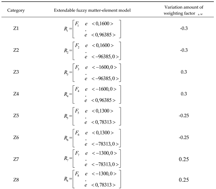
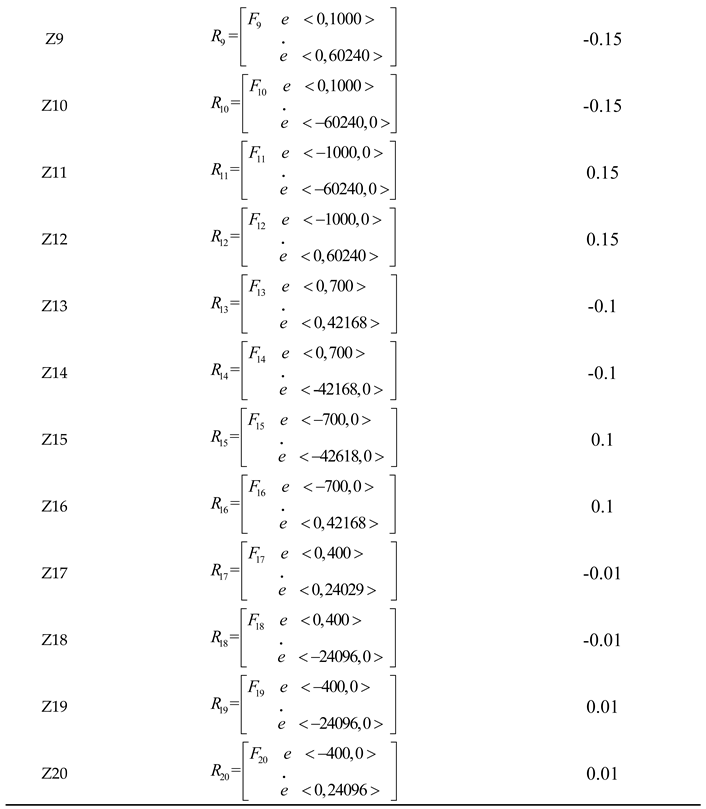
In Section 3.2, the simulation results indicated that upon the existence of nonlinear factors and parameter variation in the system, the fixed weighting factors could cause system instability and oscillation easily. To allow the weight factor of the 2DOF controller for the induction motor drive system to be adjusted along with speed variation, where the balance between control performance and control force could be obtained for better effect in control, the EFT-based smart control strategy was adopted in this paper for dynamic adjustment of the weighting factors. Such control strategy divided the speed difference between the induction motor speed within the actual speed range (0rpm to 1680rpm) and its speed command , and the variation rate for such speed difference into 20 categories. From Figure 10, it can be observed that the command error in speed difference was greater in categories Z1~Z4, hence the greater oscillation in amplitude. The command error in speed difference was less in categories Z17~Z20, hence the less oscillation in amplitude. Taking the Z1 category for example, although the speed error continued to increase, the rate of speed change reduced progressively till such rate became zero at point M (i.e., ), yet the speed error reached the maximum value. Upon then, therefore, the weighting factor should increase for enhancing the compensation amount, which reduced the impact from parameter variation. The analysis for other categories was implemented in similar manner. Summing the above with results from dynamic analysis as per Figure 10, the matter-element models of classical domains in 20 categories were established according to extendable matter-element theory. The corresponding variation amount of weighting factor was shown in Table 2. The neighborhood domain established with the maximum and minimum value of the classical domain for each characteristic was shown as in Equation (29).
3.5. Procedures of EFT-Based Dynamic Adjustment on Weighting Factors
To achieve the purpose of dynamically adjusting the weighting factor of the robust speed controller for the induction motor drive system, the speed difference between the motor speed command and the actual speed, as well as the variation rate for such an speed difference, served as the two characteristics in this paper. Through the distance and rank value in EFT, the correlation degree with each category was calculated. The greatest correlation was selected and classified as the corresponding characteristic category for determining a suitable weighting factor. The procedures of determining weighting factors with EFT were described in details below.
Step 1: Construct the corresponding category of the matter-element model against the category of speed error and its variation rate .
Step 2: Enter the speed difference and its variation rate to be classified, where a matter-element model was established.
Step 3: Calculate the speed difference and its variation rate based on Equation (26), where the correlation function with each category was derived accordingly.
Step 4: Set the weights and of each characteristic to express the significance of each characteristic. With consideration that each characteristic contained equivalent significance in the system, the weights and were both set to 0.5, and .
Step 5: Calculate the correlation degree with each category.
Step 6: For convenience of classification, the correlation degree of each category classified was normalized with Equation (33), which set the correlation degree between <-1,1>.
where and are the maximum value and minimum value of the correlation degrees for each category classified respectively.
Step 7: With the maximum correlation degree derived from calculation, the belonging category for speed difference and its variation rate to be classified was identified. Based on the belonging category, the variation amount of weighting factor was determined, and the new weighting factor was calculated again, i.e.,
Among them, was the weighting factor corresponding to the category with the maximum correlation degree derived from calculation in the previous period.
4. Simulation Results
In this paper, Matlab/simulink was applied to simulate and verify the speed control of induction motor drive system. Considering variation for moment of inertia at , system delay at 0.02 seconds, and limited control force, the speed control of the motor drive system was simulated using two methods proposed in this paper. These methods are the robust controller with a weighting factor adjusted using EFT and the robust controller adopting a fixed weighting factor. Figure 11 displayed the responses of speed command tracking and current derived from simulation, where different weighting factors were adopted when speed increased from 1000rpm to 1100rpm. From Figure 11a, it could be observed that for waveform a derived from simulation at 0.1 seconds to 0.13 seconds with an extendable fuzzy robust controller adopted, the rising curve was close to the simulated waveform d with a fixed weighting factor of zero (w = 0). Thus, it could be known that the initial adjustment of the weighting factor of the extendable fuzzy robust controller was zero, where the increase or decrease of the weighting factor was determined through the speed difference and its variation rate afterwards. Therefore, during tracking, the speed response of the extendable fuzzy robust controller presented minor oscillation of the transient response. From this, it could be observed that the weighting factor was in balance between fast response and oscillation of suppression. Therefore, it was proved that the adoption of the extendable fuzzy robust controller could effectively select the suitable weighting factor, which prevented large oscillation caused when the fixed weighting factor of 0.93 was adopted for simulation waveform g. Moreover, the time of the steady-state response for the extendable fuzzy robust controller proposed to reach the final speed was even shorter than the speed response of simulation waveform f with a fixed weighting factor of 0.8 adopted. Figure 12 presents the speed response and current response loaded with . From Figure 12a, it can be observed that, compared to the simulation waveform d, e, f and g with a fixed weighting factor adopted, the recovery time required for load regulation of the simulation waveform a with the weighting factor adjusted in an extension manner was distinctively shorter, and the speed drop was also smaller. Summing up the above, both the speed command tracking and control performance of load regulation derived from simulation for the induction motor drive system with the extendable fuzzy robust 2DOF speed controller proposed in this paper were better than the robust 2DOF controller adopting fixed weighting factors.
5. Conclusions
To improve the control performance of a robust speed controller with a fixed weighting factor for an induction motor drive system, the extendable fuzzy robust speed controller was proposed in this paper. The proposed controller could automatically adjust the weighting factors for the robust speed controller under variations of parameters, speed commands, and load disturbances of the drive system. Despite these adjustments, the controller performance of induction motor drive systems could still be maintained. The simulation results indicated that under circumstances of parameter variation in the drive system, delay characteristics and saturated control force provided in the system, the robust controller adopting fixed weighting factor could cause oscillation in speed response easily, and affect the system stability. Based on the characteristic of speed difference and its variation rate, the robust controller adopted in this paper could dynamically adjust the weighting factor to a better value. Therefore, such controller could not only improve the response performance of speed command tracking and load regulation, but also suppress the system oscillation effectively, which reduced the impact caused by parameter variation on the system, and enhanced the system stability, hence the robustness.
Author Contributions
K.-H.C. plans the project and writes, edits and reviews it. C.-L.C. is responsible for the design of robust controller for induction motor drive. K.-H.C. manages the project. All authors have read and agreed to the published version of the manuscript.
Funding
The authors gratefully acknowledge the support and funding of this project by Industrial Technology Research Institute, Taiwan, under the Grant Number NCUT23TCE021 and NCUT23TCE009 .
Institutional Review Board Statement
Not applicable.
Informed Consent Statement
Not applicable.
Data Availability Statement
This study did not report any data.
Conflicts of Interest
The authors of the manuscript declare no conflicts of interest.
References
- Yuze, W.; Wei, Z.; Chengliu, A.; Kai, W.; Haifeng, W. The Cooperative Control of Speed of Underwater Driving Motor Based on Fuzzy PI Control. In Proceedings of the 23rd International Conference on Electrical Machines and Systems (ICEMS), Hamamatsu, Japan, 24–27 November 2020; pp. 647–651. [Google Scholar]
- Zhou, S.; Li, Y.; Shi, L.; Fan, M.; Kong, G.; Liu, J. Robust Two-Degree-of-Freedom Sliding Mode Speed Control for Segmented Linear Motors. In Proceedings of the 26th International Conference on Electrical Machines and Systems (ICEMS), Zhuhai, China, 05–08 November 2023; pp. 280–285. [Google Scholar]
- Chao, K.-H.; Li, J.-Y. An Intelligent Controller Based on Extension Theory for Batteries Charging and Discharging Control. Sustainability 2023, 15, 15664. [Google Scholar] [CrossRef]
- Falconi, F.; Capitaneanu, S.; Guillard, H.; Raïssi, T. A Novel Robust Control Strategy for Industrial Systems with Time Delay. In Proceedings of the 5th International Conference on Control and Fault-Tolerant Systems (SysTol), Saint-Raphael, France, 29 September–01 October 2021; pp. 372–377. [Google Scholar]
- Chao, K.-H.; Chang, L.-Y.; Hung, C.-Y. Design and Control of Brushless DC Motor Drives for Refrigerated Cabinets. Energies 2022, 15, 3453. [Google Scholar] [CrossRef]
- Paul, O.E.; Kucher, E.S. Synthesis of Induction Motor Adaptive Field-Oriented Control System with the Method of Signal-Adaptive Inverse Model. In Proceedings of the 21st International Conference of Young Specialists on Micro/Nanotechnologies and Electron Devices (EDM), Chemal, Russia, 29 June–03 July 2020; pp. 470–474. [Google Scholar]
- O’Rourke, C.J.; Qasim, M.M.; Overlin, M.R.; Kirtley, J.L. A Geometric Interpretation of Reference Frames and Transformations: dq0, Clarke, and Park. IEEE Trans. Energy Conv. 2019, 34, 2070–2083. [Google Scholar] [CrossRef]
- Liu, C.-H. AC Motor Control: The Principles of Vector Control and Direct Torque Control, 4th ed., Tonghua Books Co. Ltd., Taipei, Taiwan, 2007; pp. 33–217.
- Ye, C.-C. AC Motor Control and Simulation Technology: A Guidance on Mastering the Core Algorithms of Electric Vehicles and Variable Frequency Technology, 1st ed., Wunan Books, Taipei, Taiwan, 2023; pp. 11–151.
- Gupta, S.; George, S. ; Awate,V. In PI Controller Design and Application for SVPWM Switching Technique Based FOC of PMSM, In Proceedings of the Second International Conference on Trends in Electrical, Electronics, Bangalore, India, 23–24 August 2023, and Computer Engineering (TEECCON); pp. 172–177.
- Vemparala, R.R.B.; Titus, J. Performance Evaluation of an Si+SiC Based Hybrid VSI Using a Modified Space Vector Switching Pattern in a Grid Connected Inverter Application. In Proceedings of the 48th Annual Conference of the IEEE Industrial Electronics Society, Brussels, Belgium, 17–20 October 2022; pp. 1–6. [Google Scholar]
- Tapia-Olvera, R.; Beltran-Carbajal, F.; Aguilar-Mejia, O.; Valderrabano-Gonzalez, A. An Adaptive Speed Control Approach for DC Shunt Motors. Energies 2016, 9, 961. [Google Scholar] [CrossRef]
- Georgiev, Z.; Trushev, I.; Chervenkov, A. Laplace Transform Method to Transient Analysis in Magnetically Coupled Electrical Circuits. In Proceedings of the International Scientific Conference on Computer Science (COMSCI), Sozopol, Bulgaria, 18–20 September 2023; pp. 1–4. [Google Scholar]
- Lin, S.; Cao, Y.; Wang, Z.; Yan, Y.; Shi, T.; Xia, C. Speed Controller Design for Electric Drives Based on Decoupling Two-Degree-of-Freedom Control Structure. IEEE Trans. Power Electron. 2023, 38, 15996–16009. [Google Scholar] [CrossRef]
- Jo, G.-J.; Choi, J.-W. Rotor Flux Estimator Design with Offset Extractor for Sensorless-driven Induction Motors. IEEE Trans. Power Electron. 2022, 37, 4497–4510. [Google Scholar] [CrossRef]
- Indriawati, K.; Widjiantoro, B.L.; Rachman, N.R. Disturbance Observer-based Speed Estimator for Controlling Speed Sensorless Induction Motor. In Proceedings of the 3rd International Seminar on Research of Information Technology and Intelligent Systems (ISRITI), Yogyakarta, Indonesia, 10–11 December 2020; pp. 301–305. [Google Scholar]
- Guo, R.-S. A Variable Weighting Robust 2DOF Speed Controller for Induction Motor, National Tsinghua University, Taiwan, Master thesis, 1999.
- Chao, K.-H.; Liaw, C.-M. Fuzzy Robust Speed Controller for Detuned Field-orientated Induction Motor Drive. IEE Proceedings - Electric Power Appl. 2000, 147, 27–36. [Google Scholar] [CrossRef]
- Xu, H.; Li, Q.; Su, J.; Yan, L. Integration of Information Models for Industrial Intemet Based on Extenics. In Proceedings of the 5th IEEE International Symposium on Smart and Wireless Systems within the Conferences on Intelligent Data Acquisition and Advanced Computing Systems (IDAACS-SWS), Dortmund, Germany, 18–20 June 2021; pp. 1–6. [Google Scholar]
- Ma, Z.; Lang, K.; Zhang, Y.; Xing, S. Comprehensive Evaluation of Emergency Situation after Collisions at Sea Based on Extenics. In Proceedings of the 4th IEEE Advanced Information Management, Communicates, Chongqing, China, 18–20 June 2021, Electronic and Automation Control Conference (IMCEC); pp. 2042–2048.
Figure 1.
Block diagram of induction motor with FOC system.
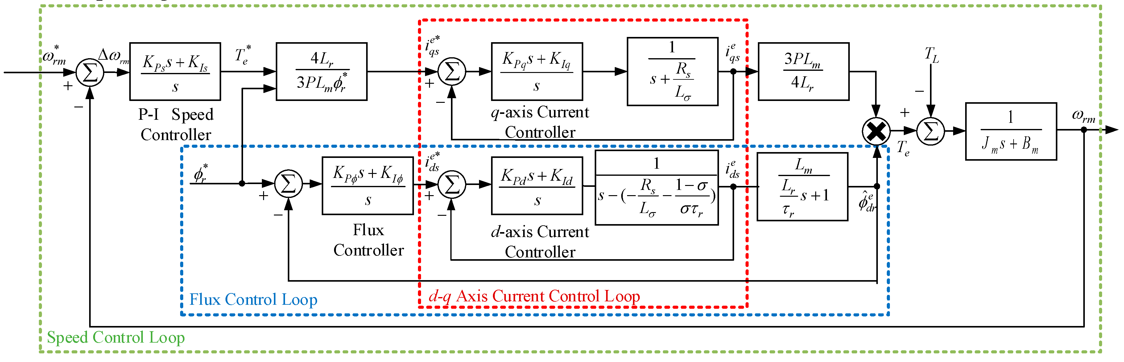
Figure 2.
Block diagram of sensorless FOC system for induction motors.
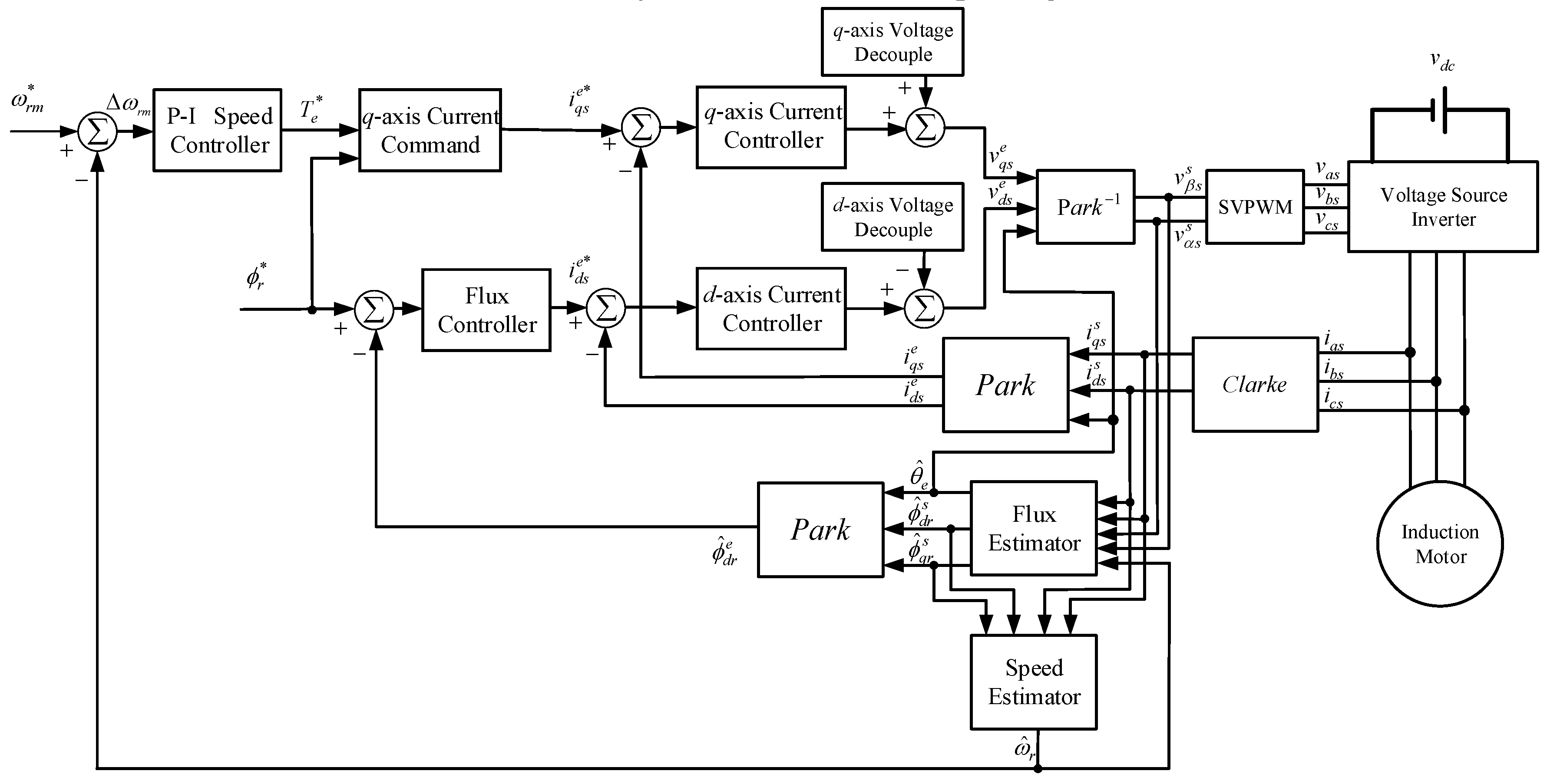
Figure 3.
Block diagram of speed control for 2DOF induction motor drive system.
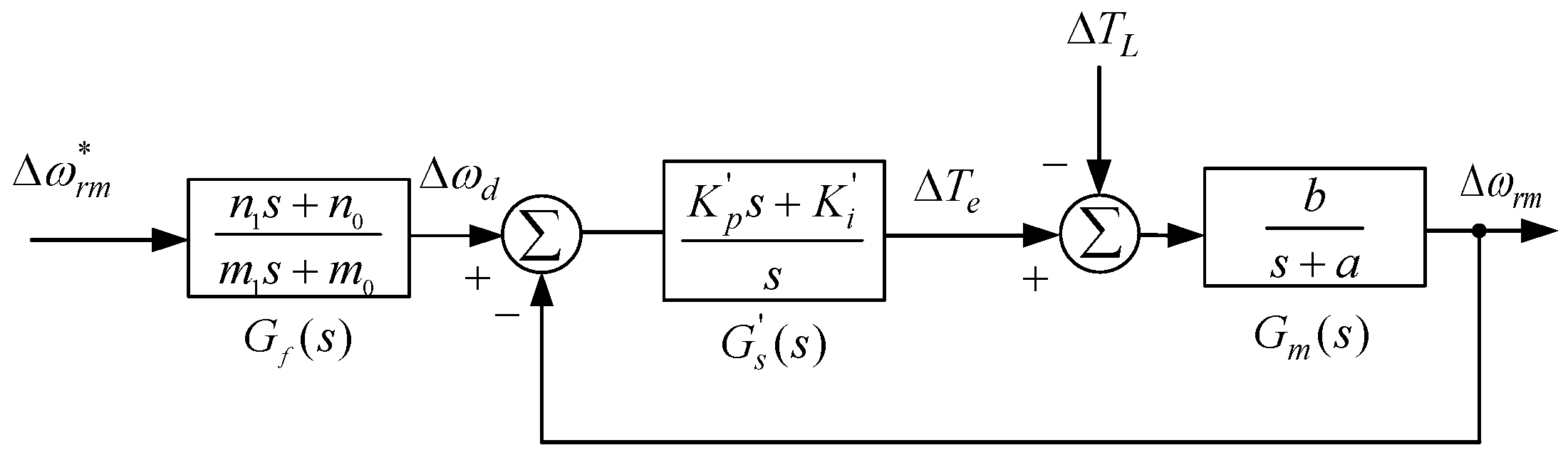
Figure 4.
Architecture of the robust 2DOF speed controller.
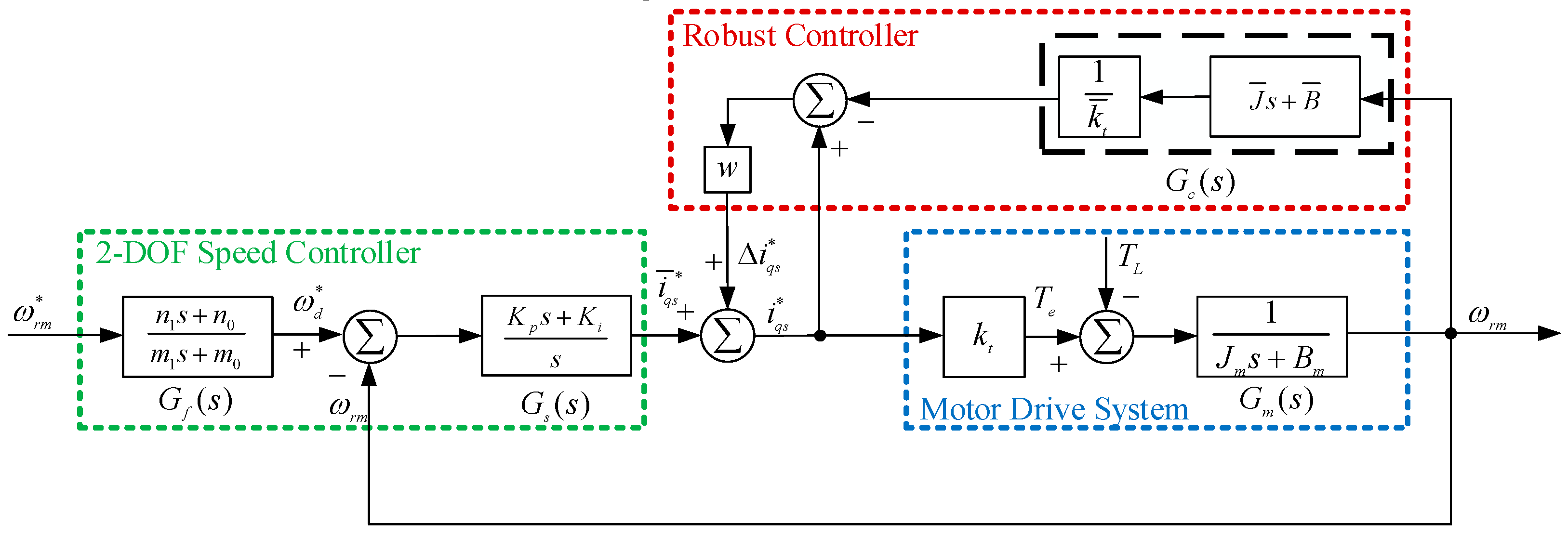
Figure 5.
The simplified block diagram of the system from Figure 4.
Figure 5.
The simplified block diagram of the system from Figure 4.
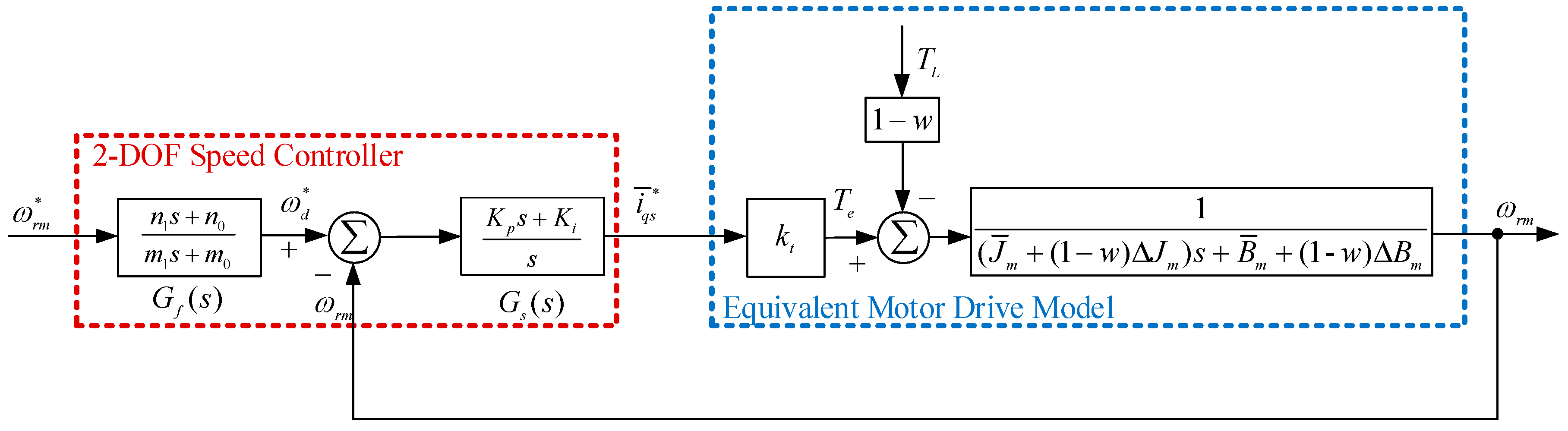
Figure 6.
Response obtained from simulation under variation of speed step command (,), where control force saturation and system delay conditions were considered: (a) Speed response; (b) Current response.
Figure 6.
Response obtained from simulation under variation of speed step command (,), where control force saturation and system delay conditions were considered: (a) Speed response; (b) Current response.
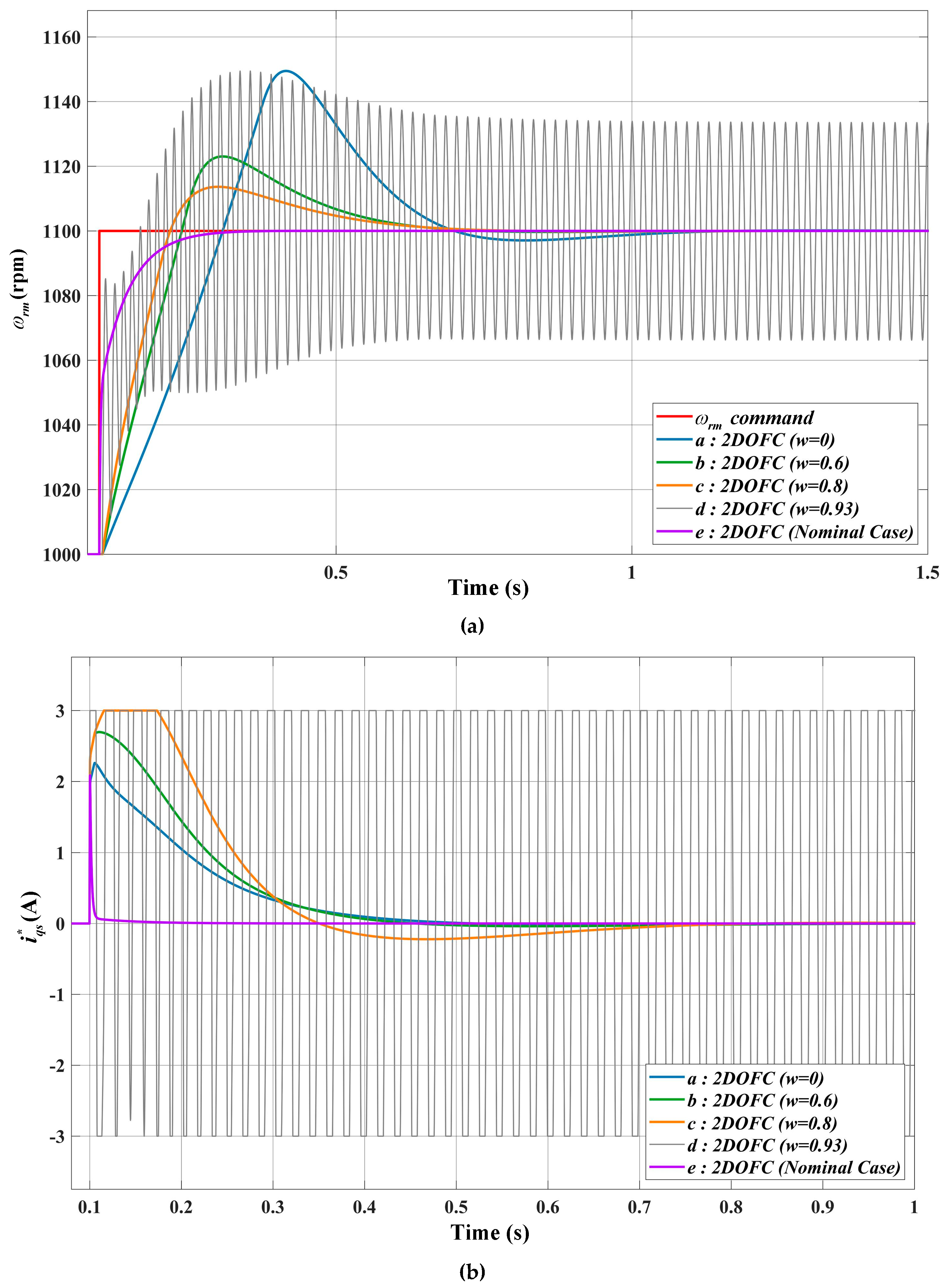
Figure 7.
Response of load regulation obtained from simulation (, ), where control force saturation and system delay conditions were considered: (a) Speed response; (b) Current response.
Figure 7.
Response of load regulation obtained from simulation (, ), where control force saturation and system delay conditions were considered: (a) Speed response; (b) Current response.
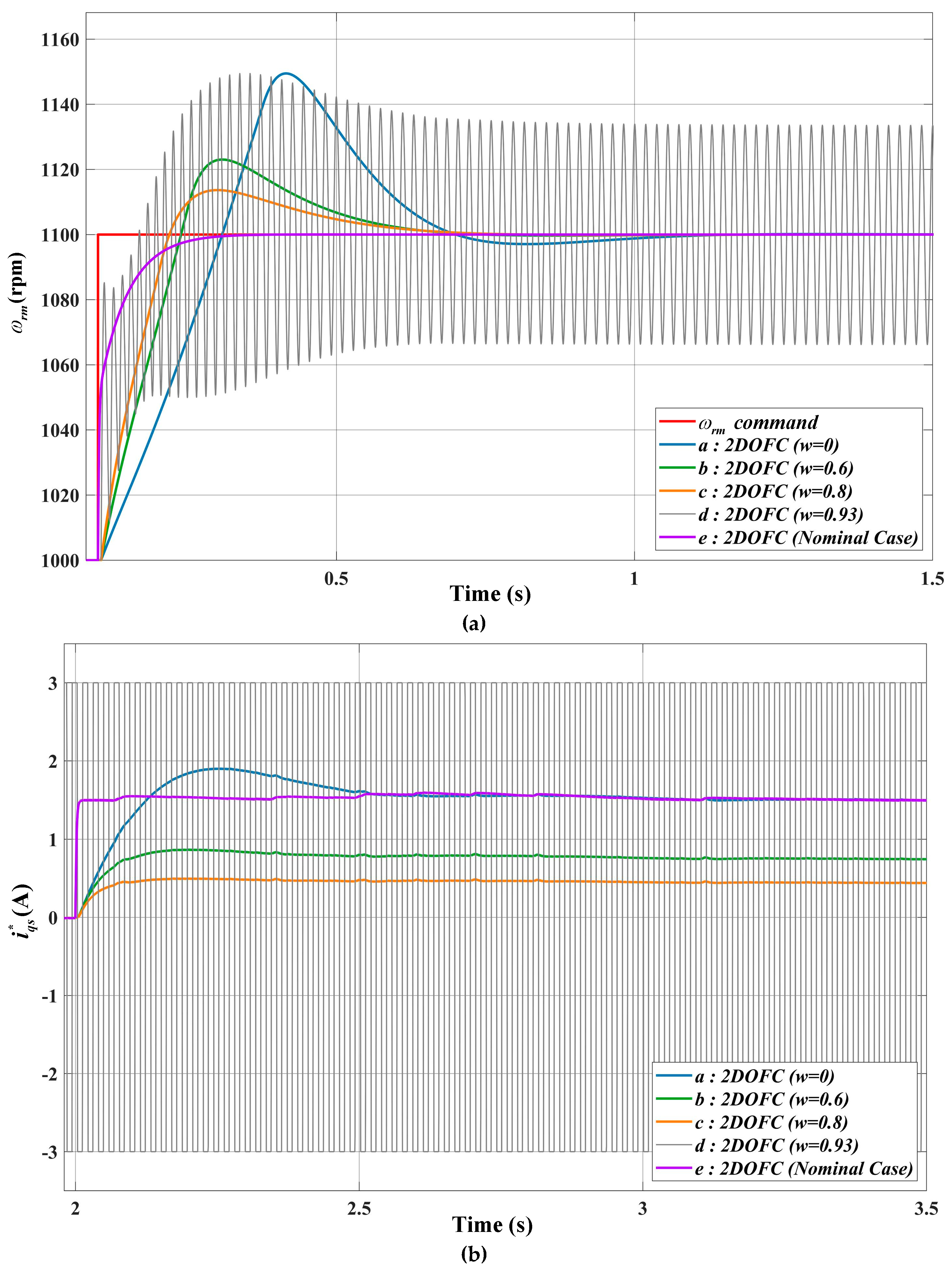
Figure 8.
System block diagram for 2DOF controller of weighting factors adjusted with EFT.
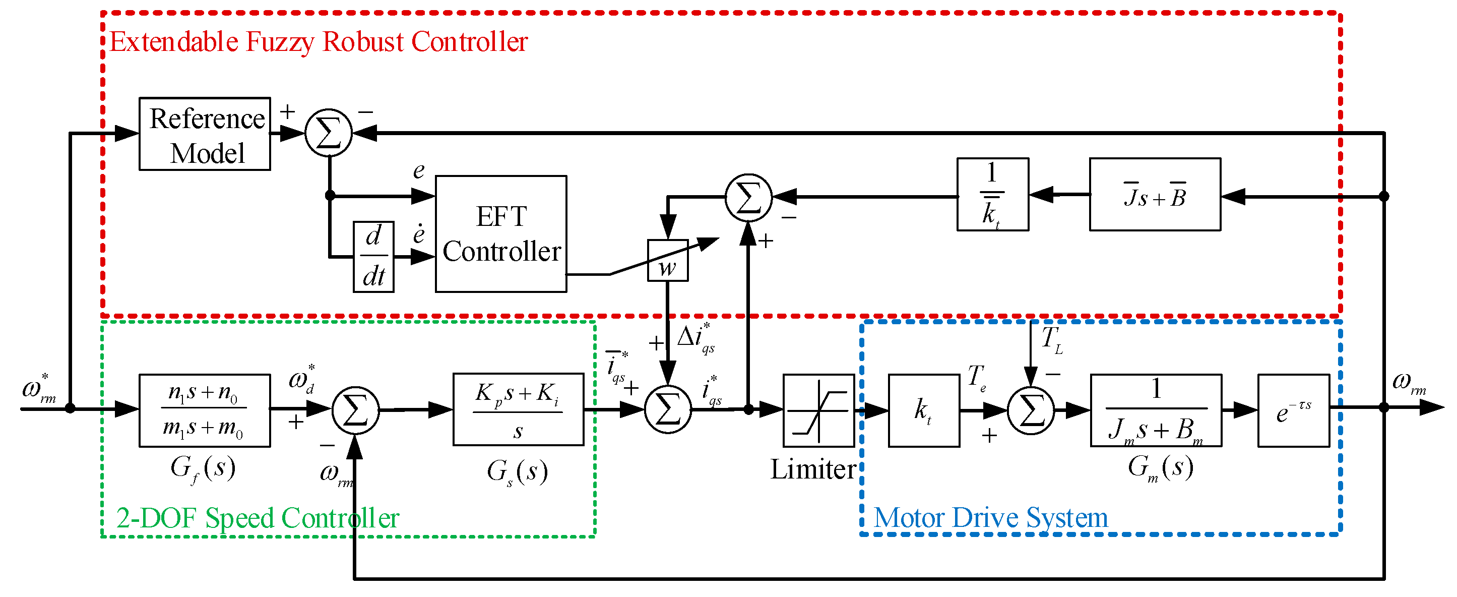
Figure 9.
Schematic of the elementary correlation function.
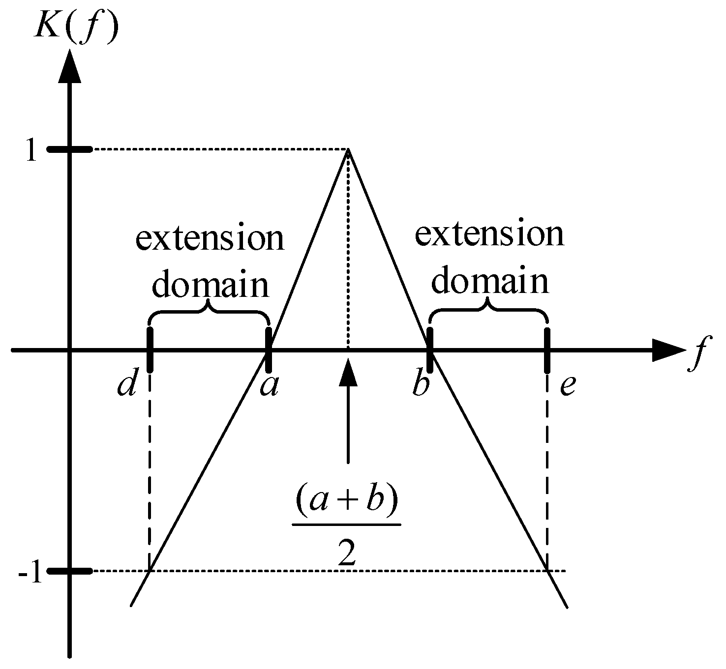
Figure 10.
Dynamic analysis of speed difference and its variation rate for induction motor.
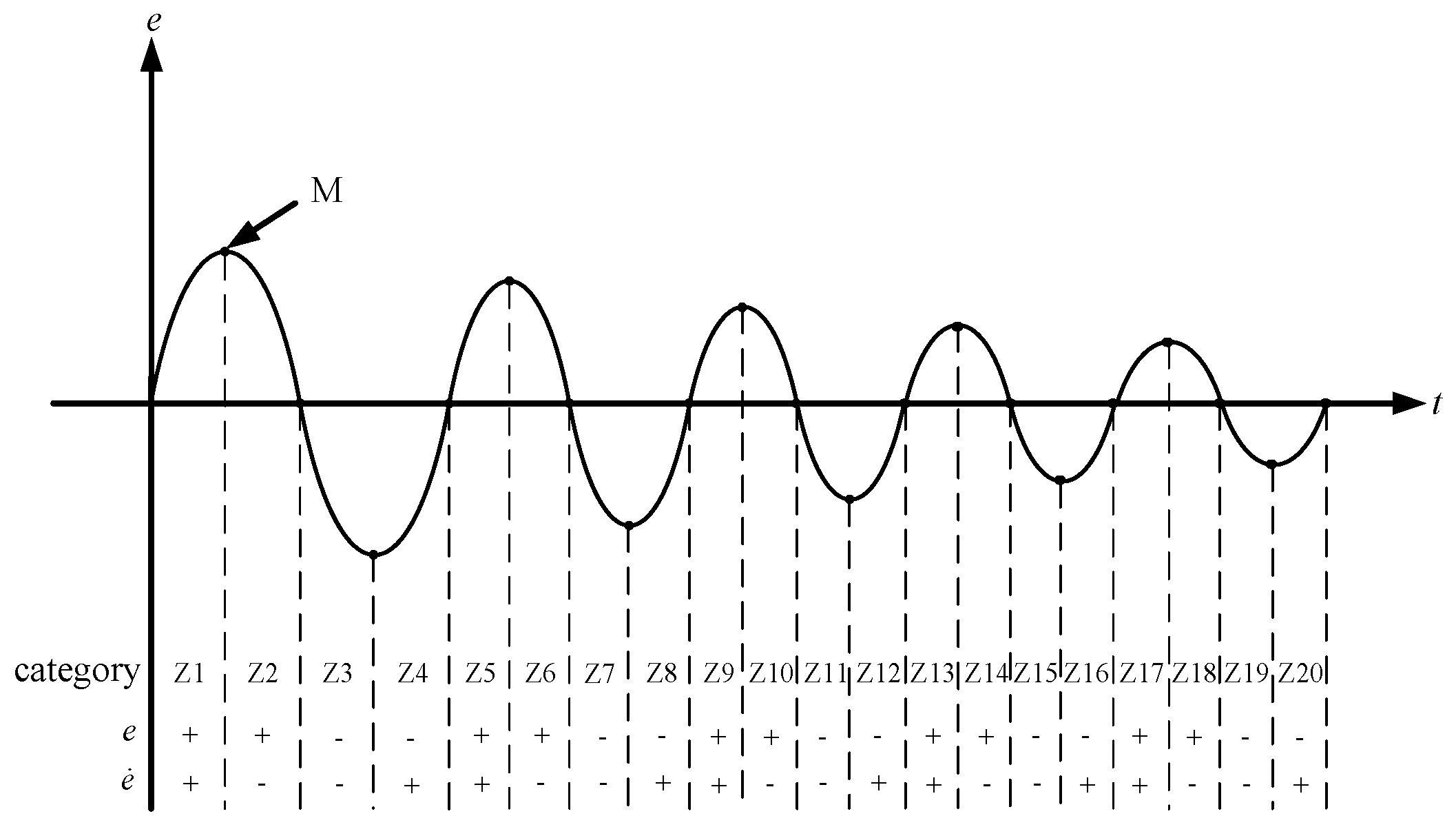
Figure 11.
Comparison of simulation results between the extendable fuzzy robust 2DOF controller proposed and robust 2DOF controller with fixed weighting factor (step command variation ): (a) Speed response; (b) Current response.
Figure 11.
Comparison of simulation results between the extendable fuzzy robust 2DOF controller proposed and robust 2DOF controller with fixed weighting factor (step command variation ): (a) Speed response; (b) Current response.
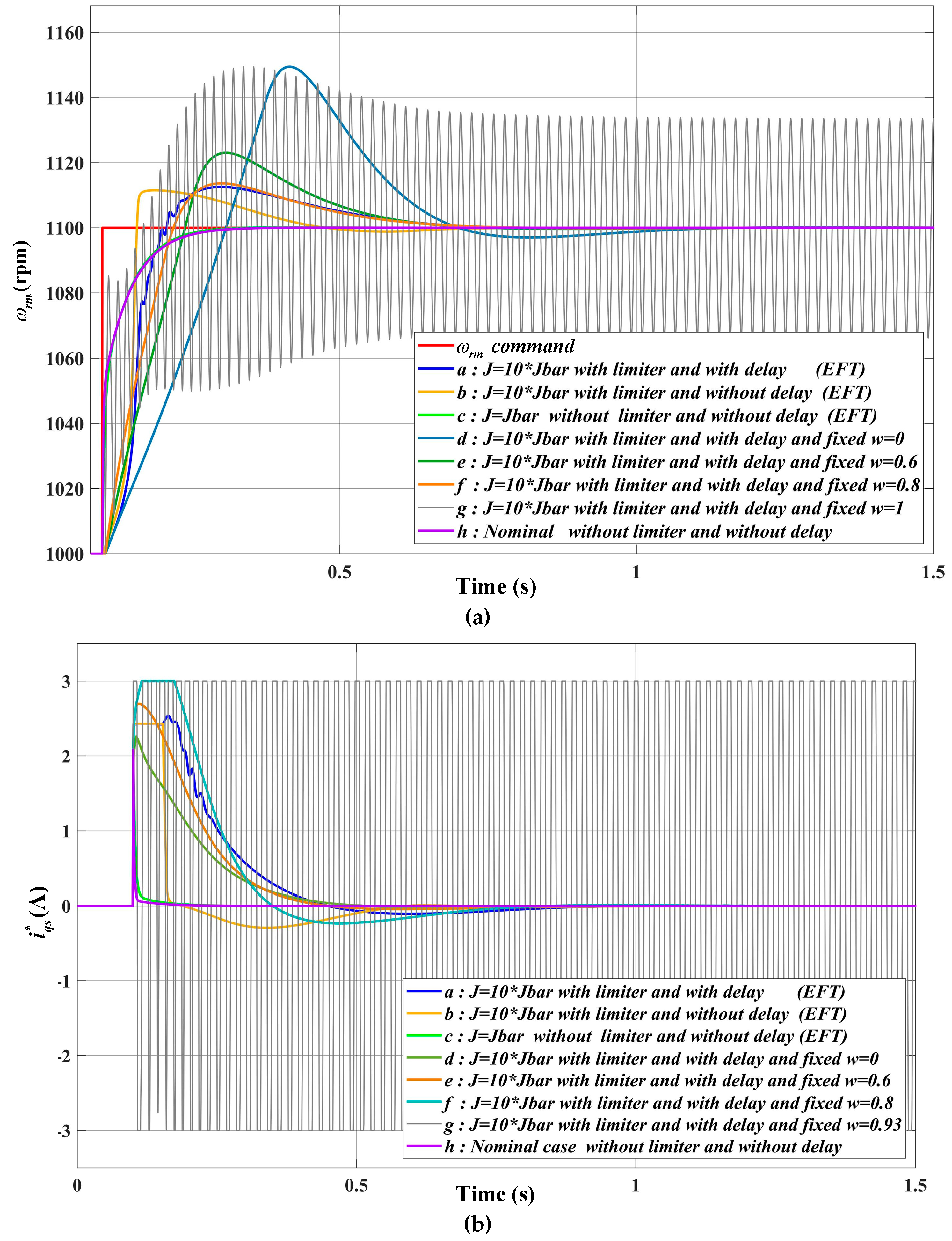
Figure 12.
Comparison of simulation results between the extendable fuzzy robust 2DOF controller proposed and robust 2DOF controller with fixed weighting factor (load disturbance ): (a) Speed response; (b) Current response.
Figure 12.
Comparison of simulation results between the extendable fuzzy robust 2DOF controller proposed and robust 2DOF controller with fixed weighting factor (load disturbance ): (a) Speed response; (b) Current response.
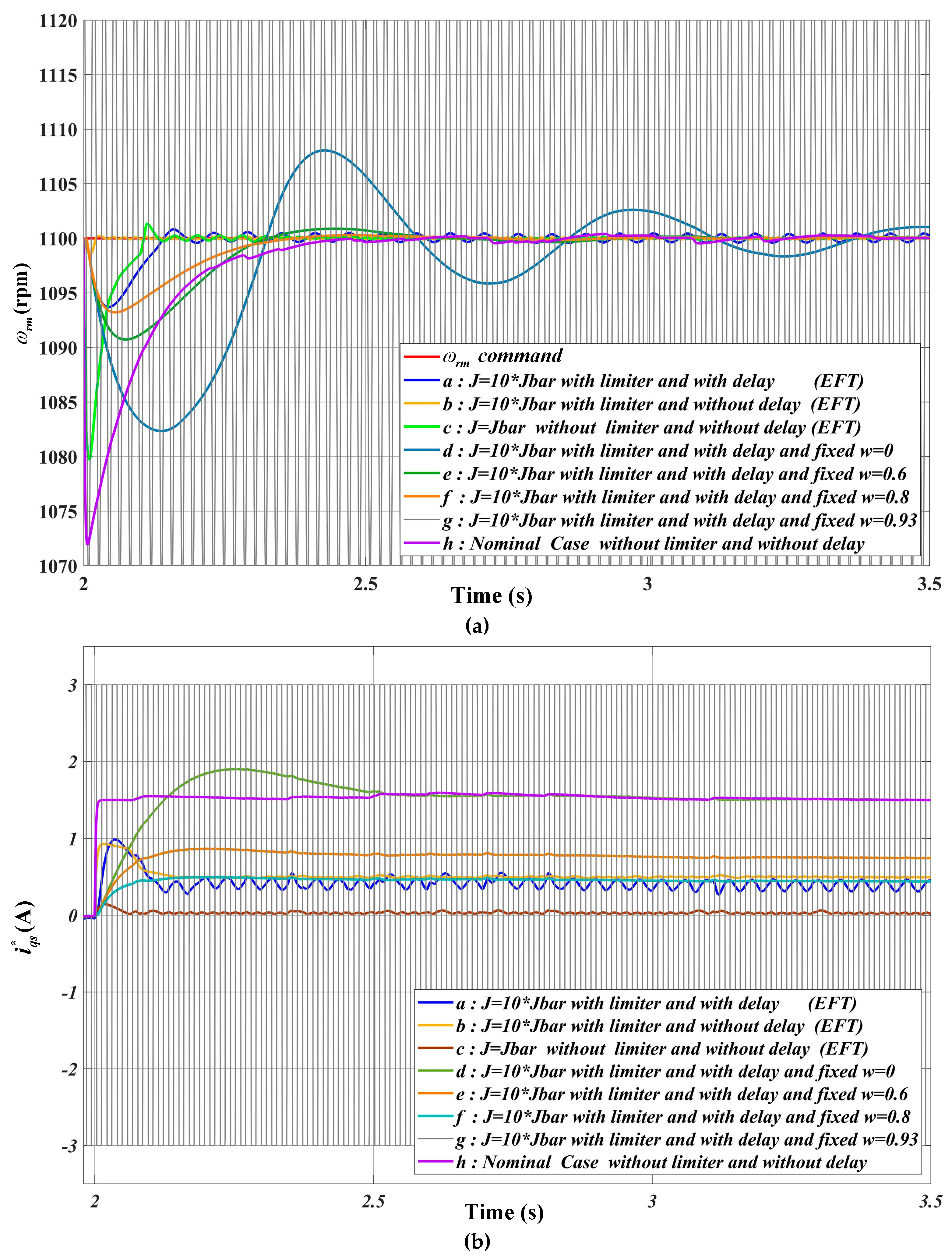

Table 1.
Three different sorts of mathematical sets.
| Compared item | Cantor set | Fuzzy set | Extendable fuzzy set |
| Research objects | Data variables | Linguistic variables | Contradictory problems |
| Model | Mathematics model | Fuzzy mathematics model | Matter-element model |
| Descriptive function | Transfer function | Membership function | Correlation function |
| Descriptive property | Precision | Ambiguity | Extension |
| Range of set | {0,1} | [0,1] | (-∞, ∞) |
Table 2.
Extendable fuzzy matter-element models in 20 categories and variation amount of corresponding weight factor.
Table 2.
Extendable fuzzy matter-element models in 20 categories and variation amount of corresponding weight factor.
Disclaimer/Publisher’s Note: The statements, opinions and data contained in all publications are solely those of the individual author(s) and contributor(s) and not of MDPI and/or the editor(s). MDPI and/or the editor(s) disclaim responsibility for any injury to people or property resulting from any ideas, methods, instructions or products referred to in the content. |
© 2024 by the authors. Licensee MDPI, Basel, Switzerland. This article is an open access article distributed under the terms and conditions of the Creative Commons Attribution (CC BY) license (http://creativecommons.org/licenses/by/4.0/).
Copyright: This open access article is published under a Creative Commons CC BY 4.0 license, which permit the free download, distribution, and reuse, provided that the author and preprint are cited in any reuse.


