Submitted:
31 May 2024
Posted:
07 June 2024
Read the latest preprint version here
Abstract
We developed a set of novel machine learning algorithms with the goal of producing transparent models (i.e. understandable-by-humans) while also flexibly accounting for nonlinearity and interactions. Our methods are based on ranked sparsity, and allow for flexibility and user-control in varying the shade of the opacity of black-box machine learning methods. In this work, we put our new ranked sparsity algorithms (as implemented in our new open-source R package, sparseR) to the test in a predictive model bakeoff on a diverse set of simulated and real-world data sets from the Penn Machine Learning Benchmarks database, including both regression and classification problems. We evaluate the extent to which our new human-centered algorithms can attain predictive accuracy that rivals popular black-box approaches such as neural networks, random forests, and SVMs, while also producing more interpretable models. Using out-of-bag error as a meta-outcome, we describe the properties of data sets in which human-centered approaches can perform as well as or better than black-box approaches. We find, interpretable approaches predicted optimally or within 5% of the optimal method in most real-world data sets. We provide a strong rationale for including human-centered transparent algorithms such as ours in predictive modeling applications.
Keywords:
model selection
; feature selection
; lasso
; explainable machine learning
1. Introduction
Since Breiman’s 2001 tale of two cultures [1], the dichotomy between black-box prediction and “transparent” statistical models has been the topic of much debate in data science. Black-box models are thought to mirror the truly ethereal data generating mechanisms present in nature; Box’s “all models are wrong” aphorism incarnated into the modeling algorithm itself. These opaque approaches are not traditionally interpretable. Transparent models, on the other hand, we define as traditional statistical models expressed as a linear combination of a maximally parsimonious set of meaningful features. Transparency is reduced with more features, features that are difficult to interpret (like interactions and polynomials), complex transformations, and of course moreso by any mix of these. Under this definition, transparency is a spectrum where the most transparent model is the “null” model (where new predictions are all set to the expected outcome in the population), followed by single-predictor models which are often called “descriptive’ models. Our definition resembles that for typical applications of Occam’s Razor in model selection where the number of parameters in the model translates directly to its simplicity, except that we consider some parameters (interactions, for instance) less transparent than others.
If accurate prediction is the goal, it is commonly thought, a model need not be traditionally interpretable. On the contrary, if it helps prediction, the predictors should be allowed to interact freely and nonlinearly in unfathomable ways; who are we humans to impart our will that the inner-workings of a model be understandable?
This paper challenges the notion that less transparency actually leads to improvements in predictive accuracy. We have developed an algorithm called the sparsity-ranked lasso (SRL) which prefers transparent statistical models [2], and shown that it outperforms other methods for sifting through derived variables like polynomials and interactions (both when such relationships truly have signal and moreso when they do not). In this work we will benchmark the performance of the SRL on X data sets from the Penn Machine Learning Benchmarking (PMLB) Database [3], Olson et al. [4], and measuring the extent to which a model’s predictive performance suffers (if it does at all). We hypothesize that in many cases, transparent modeling algorithms actually produce better models, and in most cases, they perform comparably to black-box alternatives.
Our paper is organized as follows. We first provide a brief overview of the SRL and related methodologies as well as a description of the black-box methods we will use for comparison. We then describe the benefits of transparent approaches over black-box approaches from a variety of perspectives. In our results section, we describe the data set characteristics and present our model performance both overall and then diving deeper in several illustrative case studies. We conclude with a discussion of our findings in context, describing limitations and suggestions for future work.
2. Materials and Methods
2.1. Sparsity-Ranked Lasso
Opening Pandora’s box of derived variables, also known as feature engineering, can turn any medium-dimensional problem into an exceptionally high dimensional one. Even if we restrict these derived variables to include only pairwise interactions or polynomials of existing features, the number of candidate variables grows combinatorically with the number of features, p. Therefore, we developed a high-dimensional solution to this problem: the sparsity ranked lasso.
The SRL was developed as an algorithm based on the Bayesian interpretation of the lasso [5] to favor transparent models (i.e., models with fewer interactions and polynomials). The SRL initially resembles the adaptive lasso [6], wherein we optimize the function Q for the parameters of interest which measure the associations between the outcome y and the columns of a covariate matrix X. The hyperparameter represents the extent of overall shrinkage towards zero, and the nature of the discontinuity renders some estimated coefficients exactly zero, inherently deselecting them from the model. The lasso and the SRL are both typically tuned using model selection criteria or cross-validation.
The SRL uses penalty weights to increase the skepticism for columns of X corresponding to interactions and polynomials, which (if selected) would render the model more opaque. We have shown that setting for all j, where represents the size of the set of covariates, sets the prior information contributed by interactions to be equal to that of main effects, while also naturally inducing skepticism (higher penalties) on interactions without having to tune additional hyperparameters. The SRL is currently implemented in the sparseR R package available on the Comprehensive R Archive Network (CRAN). The SRL can successfully sift through a large, high-dimensional set of possible interactions and polynomials while still preferring transparency, in contrast to alternative methods which tend to over-select interactions and higher-order polynomials [2]. The binomial loss function replaces the least-squares term in the above equation when the outcome is binary.
2.2. Black-Box Algorithms
In this work we primarily utilize the (arguably) black-box supervised learning algorithms briefly described in this section. Random forest algorithms [7] are an ensemble-based learning method for continuous and categorical endpoints. They operate by constructing many candidate decision trees using bootstrapped & sub-sampled training data, predicting the outcome as the mode of the classes (classification) or mean prediction (regression) of the individual trees. Whereas individual trees (weak learners) may over- or under-fit the training data, using an ensemble improves predictions by averaging multiple decision trees. Support Vector Machines (SVMs) [8] work by finding the hyperplane that best separates observations in the feature space. SVMs are effective in high-dimensional spaces and are particularly useful for cases where the number of dimensions exceeds the number of samples. Extreme Gradient Boosting (XGBoost) [9] is an efficient implementation of the gradient boosting framework. Similarly to random forests, XGboost builds an ensemble of trees, except it does so in a sequential manner, where each tree tries to correct the errors of the previous one. XGBoost also incorporates regularization to prevent overfitting. Neural networks [10,11] are a set of algorithms inspired by the structure and function of the human brain, designed to recognize patterns. They consist of layers of nodes (neurons) that process input data and pass it through successive layers. Each node assigns weights to its inputs and passes them through an activation function to determine the output. This extremely flexible set-up makes neural networks capable of modeling complex, non-linear relationships. They work particularly well at text, image, and speech recognition.
2.3. Issues with Black-Box Algorithms
In classical statistical modeling, the overarching objective is often delineated as either descriptive or predictive. Descriptive modeling focuses on providing a succinct, interpretable characterization of how a set of explanatory variables is jointly associated with the outcome, with the primary inferential goal centered on the estimation and inference of effects (i.e., regression parameters). Predictive modeling focuses on the accurate approximation of new outcomes. A commonly held perspective is that transparency is only an important consideration with descriptive modeling. With large samples, predictive accuracy generally improves as more nuanced and subtle effects are added to the model, leading to a less parsimonious and less interpretable model structure. Black-box algorithms are built upon the philosophy that reality is too complex to succinctly encapsulate with a transparent model structure, and that optimal prediction is best accomplished by sacrificing interpretability in order to mirror the intricacies and sophistication of reality.
However, in many modeling applications, even if prediction is the primary goal, description is still an important secondary objective. Investigators are generally not only concerned with the quality of the predictors, but also with the manner in which they are derived. The lack of transparency of black-box algorithms can be problematic in critical applications such as healthcare, finance, and insurance, where decisions should be justifiable and explainable, as well as in the development of modern technological innovations, such as autonomous vehicles, smart devices, and large language models (LLMs). For example, in criminal justice, the General Data Protection Regulation (GDPR) provides a legal framework that sets guidelines for the collection and processing of personal information from individuals who live in and outside of the EU. Adherence to such guidelines may be difficult to achieve by opaque algorithms, which suffer from algorithmic bias and tend to propagate systematic discrimination or disparities. Because of this, rather than building trust in science, OMs tend to either erode trust for some while producing excessive trust in others.
Due to their complexity, black-box algorithms can also be difficult to debug or troubleshoot. A related problem is that black-box models may degrade over time due to changes in the data distribution (“concept drift”). Detecting and adapting to the evolution of the data-generating mechanism can be challenging if one is unaware as to which model structures are impacted by the resulting changes.
Additionally, black-box algorithms are prone to overfitting, and may therefore perform much more effectively in predicting training data than validation data. Moreover, if the features used to build the algorithm are extracted through an automated search as opposed to scientific knowledge, features that are spuriously associated with the outcome may naturally enter the model. Such features may degrade the quality of the prediction if conditions lead to a disconnection in the association. For instance, since the flu season generally coincides with the college basketball season, the number of college basketball games played in a given week during the flu season is typically highly correlated with flu incidence during the same week. However, during atypical flu seasons, such as the 2009 H1N1 pandemic, this association will disappear.
Our philosophy is that a certain degree of complexity is often warranted for high quality prediction. Yet a model that is primarily based on meaningful, pronounced features, and only incorporates more nuanced and subtle features if the evidence provided by the data is sufficiently compelling to warrant their inclusion, will often be transparent and interpretable. Moreover, such a model will generally perform as well as or better than black-box methods that disregard the principle of parsimony and potentially violate Occam’s Razor.
2.4. PMLB Processing Steps
PMLB data sets were loaded using the pmlbr R package [12]. Metadata including predictor types, endpoint types, and feature counts were extracted from the PLMB GitHub (https://github.com/EpistasisLab/pmlb) repository using GitHub’s API. We restricted analysis data sets to those with binary or continuous endpoints (categorical endpoint sets were discarded), with fewer than 10,000 observations, with 50 or fewer predictors, and fewer than 100,000 total predictor cells (predictor columns times observations). Friedman simulated data sets were also removed. For categorical variables, all classes that appeared in less than 10% of observations were combined into a single class. Prior to modeling, all data sets were split into training and test sets where approximately 20% of observations were set aside in the test set. For each data set, all models were fit and evaluated using the same training and test sets.
2.5. Modeling Procedures
All random forest, SVM, neural network, and XGBoost models were fit using 10-fold cross-validation (CV) and grid search to tune hyper-parameters. For random forests, values between 2 and p, where p is the number of predictors for a given data set, were evaluated as candidates for the count of random predictors to be used for each split. SVM models were fit using a cost of constraints violation of 1. For neural networks, hidden layer sizes from 1 to 5 and weight decays from 0 to 0.1 were considered during grid search. For XGBoost, grid search considered maximum tree depths of 1 to 3, learning rate from 0.3 to 0.4, subsampled column ratios of 0.6 to 0.8, boosting iterations from 50 to 150, and training subsample ratios of 0.50 to 1.
For continuous endpoints, CV R-squared, test R-squared, and test root mean squared error (RMSE) were calculated for each combination of algorithm and PMLB data set. For binary endpoints, test area under the receiver operating characteristic curve (AUC) was calculated for each combination of algorithm and PMLB data set. In some cases, R-squared was unable to be calculated for neural networks, in those instances R-squared was set to zero.
3. Results
3.1. Data Set Characteristics
Descriptive statistics for our sampled PMLB data sets are presented in Table 1 for the overall sample and stratified by endpoint type. The size of data sets (number of samples vs number of features) is visualized in Figure 1, showing a fairly uniform distribution along our studied range of features and sample sizes for both categorical and continuous endpoint types. On average, data sets had 5 categorical features (SD: 7), and 5 continuous features (SD: 6).
3.2. Overall Model Performance
Descriptive results for model performances are shown in Table 2. For continuous endpoints, the lasso and SRL had the best-performing model for test data in 15.4% and 23.1% of data sets (totaling 38.4%), and the SRL was within 5% out-of-sample predictive accuracy of the best performing model in two thirds of data sets. For binary endpoints, the lasso and SRL performed best in 22.7% and 34.8% of data sets (totaling 57.5%), and the SRL was within 5% of the best model in 69.7% of data sets. The and SRL were generally faster than black-box methods.
Inferential results comparing models in terms of CV-based R-squared, out-of-sample R-squared, and out-of-sample AUC are displayed in Table 3 and summarized in Figure 2. The SRL generally performed slightly better than the lasso (though this difference was only significant for binary endpoints, where SRL had test-set AUCs 0.04 points higher (95% CI: 0.01-0.06; p = 0.018). Similarly, the SRL generally performed better than neural networks, though this difference was only significant for the out-of-sample R-squared for continuous endpoints, where SRL had R2 values 0.07 points higher (95% CI: 0.01-0.13; p = 0.016). Random forests and XG-boosting performed generally better than SRL in terms of CV-based R-squared, however both comparisons becomes insignificant in out-of-sample endpoints. Finally, the SRL performed significantly better than SVMs for binary endpoints, with AUCs on average 0.13 units higher (95% CI: 0.10-0.16; p < 0.001).
Figure 3 displays a comparison of random forests to the SRL in terms of out-of-sample performance for all data sets. Here we note that random forests and SRL perform similarly on the majority of data sets. There are a handful of cases in which random forests highly outperform the SRL. A subset of data sets denoted in Figure 3 as red points will be investigated in the next section as illustrative case studies.
3.3. Case Studies
Here we present 7 case studies, starting with two exemplars of the pattern evident in Figure 3 where SRL and random forest models perform similarly, and concluding with 5 outliers where SRL seems to be underperforming relative to random forests.
3.3.1. Exemplars
For the 503_wind data set, performance was similar between SRL and other methods, but SRL outperformed all other methods in terms of test R-squared and test RMSE with a notably faster run time than random forest, SVM, and neural network. Results for the 503_wind data set are provided in Table 4.
Not only did SRL have the best performance among the comparison set, it also produces parameter estimates which are interpretable. In Figure 4, we present effect of three types of significant relationships found by SRL in the 503_wind data: linear, linear with an interaction effect, and a non-linear effect.
For the hungarian data set, SRL was the fourth best performing model in terms of ROC AUC, however the performance of the top four models was extremely close with each having an AUC with 0.032 of one another. Results for the hungarian data set are provided in Table 5.
While SRL did not outperform random forest for this data set, it does provide interpretable parameter estimates relative to random forest for only a marginal reduction in performance. In Figure 5, we present effect of two types of significant nonlinear relationships found by SRL in the hungarian data: an interaction effect and a quadratic effect.
3.3.2. SRL Underperforming RF
In this section we delve more deeply into examples where SRL appears to be performing worse than alternative methods (case studies highlighted in Figure 3).
…
4. Discussion
We are not the first to suggest that transparent modeling methods perform comparably to black-box methods; Christodoulou et al. [13] found that when aggregating across biomedical data sets from 71 real studies, logistic regression performed on average exactly the same as black-box alternatives.
Data sets are growing increasingly large and diverse, and the subset of data set examples we explored in the PMLB, while larger than any previous study comparing such methods, is limited in generalizability to data sets with similar outcomes, number of features, signal-to-noise ratios, and variable distributions. In particular, we cannot generalize these findings to especially high-dimensional data sets (p > 40), or massive data sets (n > 10,000 or n*p > 100,000) as these were not included in our analysis. This comparison and extension would be welcome future work, as black-box models are said to be data hungry, performing best in these massive data settings [14]. However, this extension would require improved scalability of various methods as currently implemented.
We did not investigate the implementation of stacking or other ensemble-based approaches [cite]. Under our definition of transparency, such approaches are not transparent. Therefore, if a transparent model fits the data best, it will improve the performance of black-box ensembles, but at (in our view) a high cost of reduced interpretability. Still, in practice it is advisable to fit such an ensemble and compare its performance to transparent methods alone. One can compare the relative weight of transparent methods against black-box alternatives to map the data-set-specific tradeoff between predictive accuracy and transparency, and then make decisions regarding whether an observed improvement in performance (if it exists) is worth the opacity and its potential issues regarding trust, fairness, stability, etc.
5. Conclusions
Our transparent algorithms sometimes predict better than black-box counterparts and most of the time perform comparably At least for comparable data sets, e.g., not necessarily huge data sets. We stress modelers to always at least consider a transparent model.
Data Availability Statement
All code & data used are available upon request from the authors.
Acknowledgments
No funding is declared for this work.
Conflicts of Interest
The authors declare no conflict of interest.
Abbreviations
The following abbreviations are used in this manuscript:
| MDPI | Multidisciplinary Digital Publishing Institute |
| DOAJ | Directory of open access journals |
| SRL | Sparsity-ranked lasso |
References
- Breiman, L. Statistical Modeling: The Two Cultures (with comments and a rejoinder by the author). Statistical Science 2001, 16, 199–231. [Google Scholar] [CrossRef]
- Peterson, R.A.; Cavanaugh, J.E. Ranked Sparsity: A Cogent Regularization Framework for Selecting and Estimating Feature Interactions and Polynomials. AStA Advances in Statistical Analysis 2022, 106, 427–454. [Google Scholar] [CrossRef]
- Romano, J.D.; Le, T.T.; La Cava, W.; Gregg, J.T.; Goldberg, D.J.; Chakraborty, P.; Ray, N.L.; Himmelstein, D.; Fu, W.; Moore, J.H. PMLB v1.0: An open source dataset collection for benchmarking machine learning methods. arXiv preprint arXiv:2012.00058v2, arXiv:2012.00058v2 2021.
- Olson, R.S.; La Cava, W.; Orzechowski, P.; Urbanowicz, R.J.; Moore, J.H. PMLB: A large benchmark suite for machine learning evaluation and comparison. BioData Mining 2017, 10, 1–13. [Google Scholar] [CrossRef] [PubMed]
- Tibshirani, R. Regression Shrinkage and Selection via the Lasso. Journal of the Royal Statistical Society: Series B 1996, 58, 267–288. [Google Scholar] [CrossRef]
- Zou, H. The adaptive lasso and its oracle properties. Journal of the American statistical association 2006, 101, 1418–1429. [Google Scholar] [CrossRef]
- Breiman, L. Random forests. Machine learning 2001, 45, 5–32. [Google Scholar] [CrossRef]
- Cortes, C.; Vapnik, V. Support-vector networks. Machine learning 1995, 20, 273–297. [Google Scholar] [CrossRef]
- Chen, T.; Guestrin, C. Xgboost: A scalable tree boosting system. Proceedings of the 22nd acm sigkdd international conference on knowledge discovery and data mining, 2016, pp. 785–794.
- Liaw, A.; Wiener, M. Classification and Regression by randomForest. R News 2002, 2, 18–22. [Google Scholar]
- Goodfellow, I.; Bengio, Y.; Courville, A. Deep Learning; MIT Press, 2016. http://www.deeplearningbook.org.
- Le, T. ; makeyourownmaker.; Moore, J. pmlbr: Interface to the Penn Machine Learning Benchmarks Data Repository, 2023. [Google Scholar]
- Christodoulou, E.; Ma, J.; Collins, G.S.; Steyerberg, E.W.; Verbakel, J.Y.; Van Calster, B. A systematic review shows no performance benefit of machine learning over logistic regression for clinical prediction models. Journal of Clinical Epidemiology 2019, 110, 12–22. [Google Scholar] [CrossRef] [PubMed]
- van der Ploeg, T.; Austin, P.; Steyerberg, E. Modern modelling techniques are data hungry: A simulation study for predicting dichotomous endpoints. BMC Med Res Methodol 2014, 14, 137. [Google Scholar] [CrossRef] [PubMed]
Figure 1.
PMLB Data Set Size.
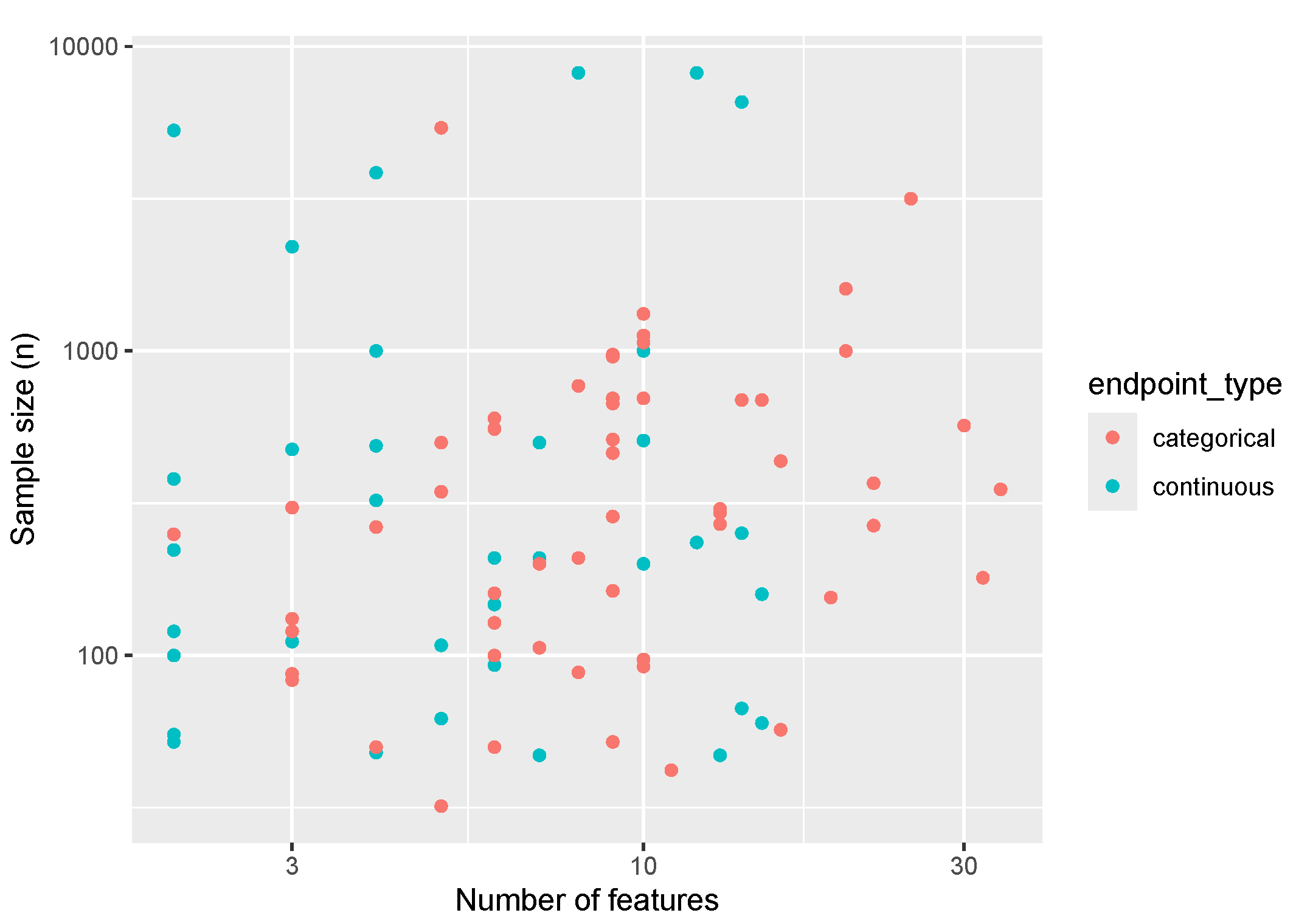
Figure 2.
LMM contrasts for predictive accuracy compared to SRL.
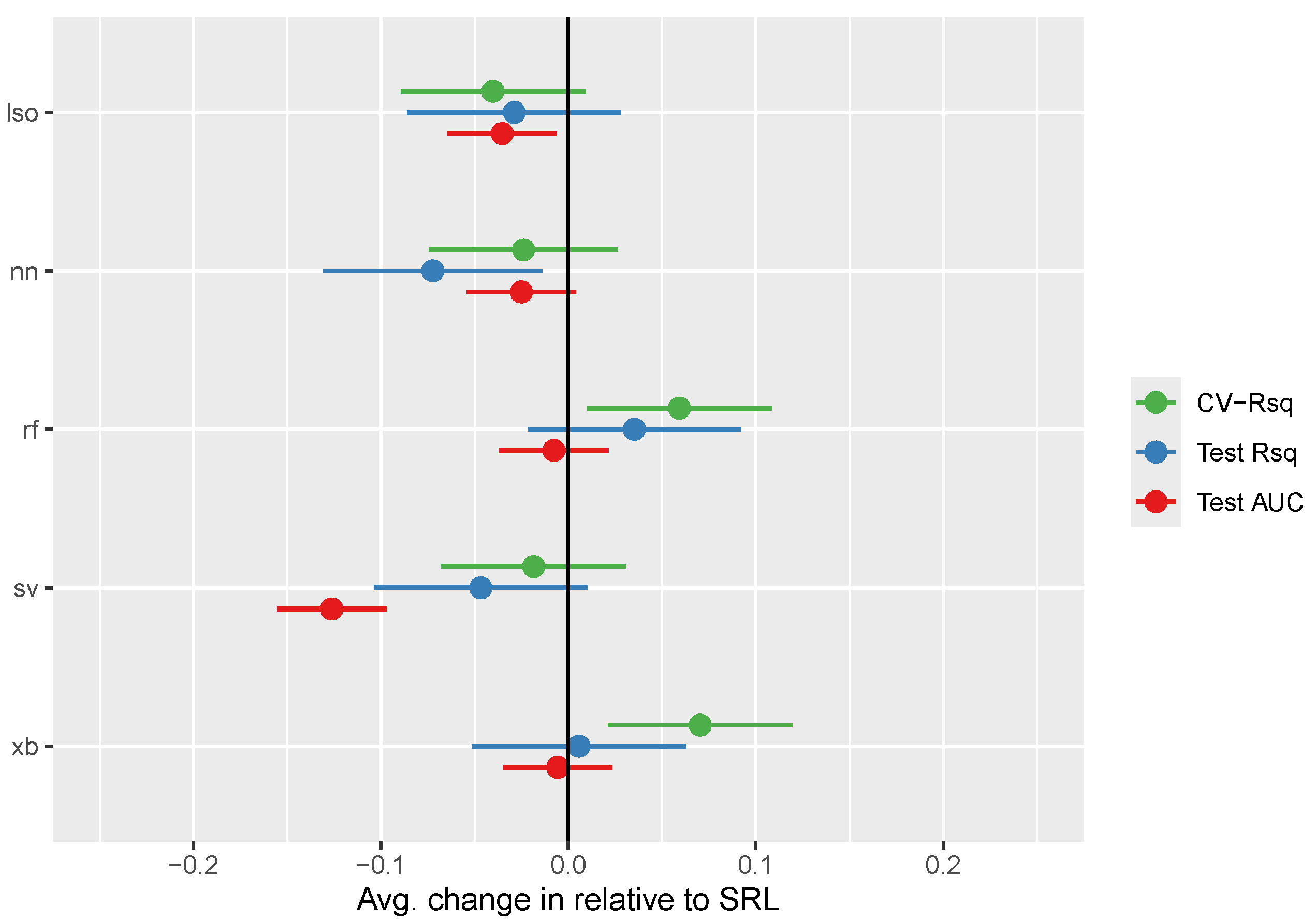
Figure 3.
Comparing random forests to SRL. Each point represents a data set.
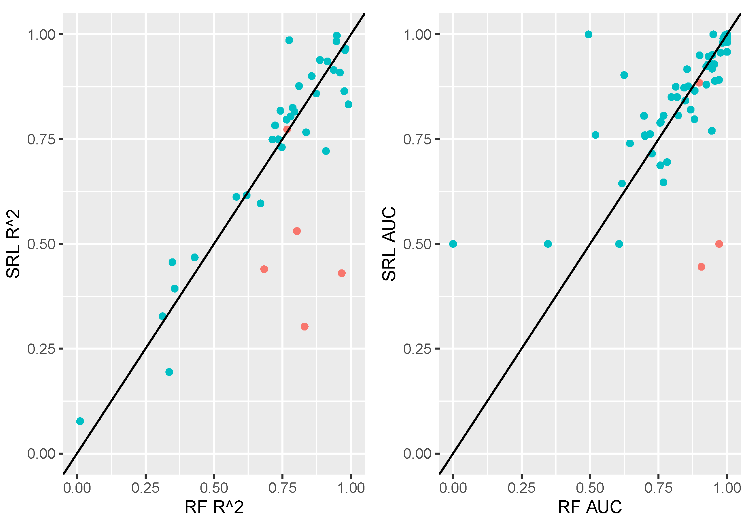
Figure 4.
For the 503 wind data set, SRL discovered significant and interpretable linear relationships (left), interaction effects (center), and non-linear relationships (right)
Figure 4.
For the 503 wind data set, SRL discovered significant and interpretable linear relationships (left), interaction effects (center), and non-linear relationships (right)
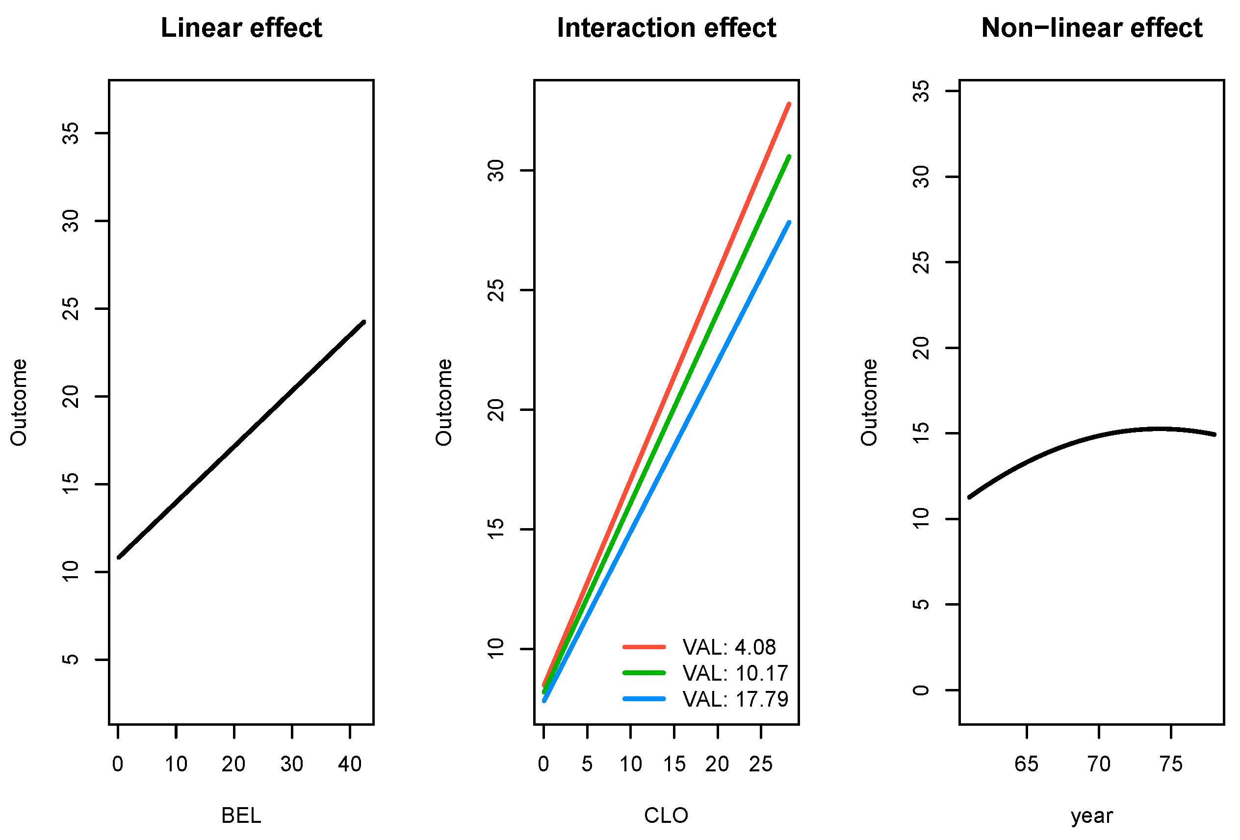
Figure 5.
For the hungarian data set, SRL discovered significant and interaction relationships (left), and a quadratic relationship (right)
Figure 5.
For the hungarian data set, SRL discovered significant and interaction relationships (left), and a quadratic relationship (right)
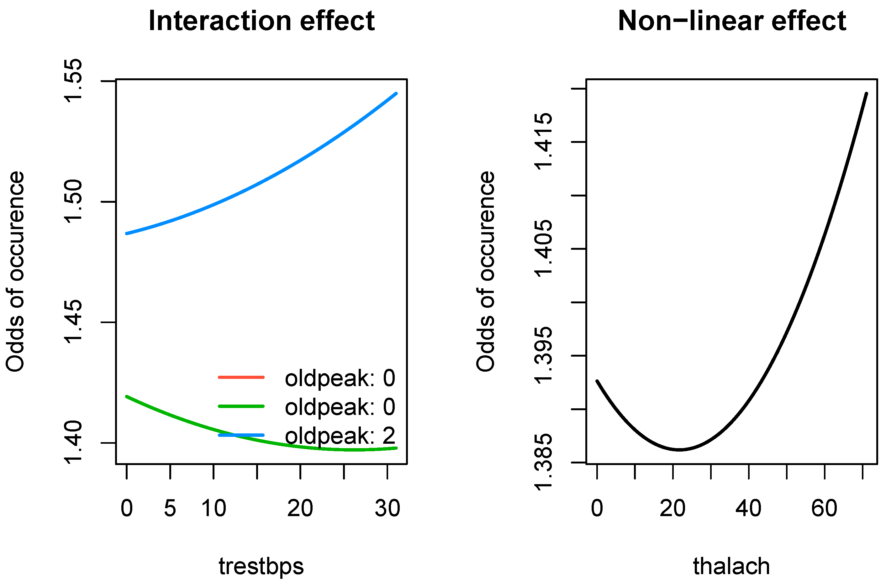

Table 1.
Sample Characteristics
| Characteristic | Overall, N = 110 | categorical, N = 69 | continuous, N = 41 |
| n_instances | 856.21 (1,619.0) | 611.93 (795.8) | 1,267.32 (2,406.2) |
| n_features | 10.15 (7.0) | 12.07 (7.6) | 6.93 (4.4) |
| n_categorical_features | 5.02 (7.0) | 7.97 (7.4) | 0.05 (0.3) |
| n_continuous_features | 5.14 (6.0) | 4.10 (6.5) | 6.88 (4.5) |
| n_classes | 148.57 (858.0) | 2.00 (0.0) | 395.24 (1,380.8) |
| imbalance | 0.08 (0.1) | 0.11 (0.2) | 0.04 (0.1) |
| 1 Mean (SD) | |||
Table 2.
Performance across all data sets.
| LSO | NN | RF | SRL | SV | XB | |
| Continuous | ||||||
| CV Rsq; mean (SD) | 65.4 (22) | 41.8 (40) | 75.4 (18) | 69.4 (23) | 67.6 (22) | 76.5 (18) |
| Test Rsq; mean (SD) | 68.1 (23) | 58.3 (29) | 74.6 (23) | 71 (24) | 66.4 (24) | 71.6 (23) |
| Best performance (%) | 15.4 | 15.4 | 33.3 | 23.1 | 2.6 | 10.3 |
| Within 5% of best (%) | 46.2 | 35.9 | 66.7 | 66.7 | 43.6 | 51.3 |
| Run time (s?); mean (SD) | 3.2 (2) | 8.1 (8) | 15.8 (17) | 4.9 (3) | 10.3 (12) | 15.1 (5) |
| Binary | ||||||
| Test AUC; mean (SD) | 82.4 (17) | 83.4 (16) | 85.1 (18) | 85.9 (15) | 73.3 (18) | 85.3 (16) |
| Best performance (%) | 22.7 | 27.3 | 37.9 | 34.8 | 6.1 | 39.4 |
| Within 5% of best (%) | 65.2 | 56.1 | 69.7 | 78.8 | 18.2 | 71.2 |
| Run time (s?); mean (SD) | 7.2 (8) | 12.7 (10) | 13.9 (14) | 11.6 (11) | 8.3 (8) | 14.9 (3) |
Table 3.
Linear Mixed (Meta) Models
| CV Rsq | Test Rsq | AUC | ||||
| Term | Estimate (CI) | p | Estimate (CI) | p | Estimate (CI) | p |
| Intercept | 69.4 (63, 76) | < 0.001 | 71 (64, 79) | < 0.001 | 85.9 (82, 90) | < 0.001 |
| LSO | -4 (-9, 1) | 0.11 | -2.9 (-9, 3) | 0.32 | -3.5 (-6, -1) | 0.018 |
| NN | -2.4 (-7, 3) | 0.35 | -7.2 (-13, -1) | 0.016 | -2.5 (-5, 0) | 0.092 |
| RF | 5.9 (1, 11) | 0.019 | 3.5 (-2, 9) | 0.22 | -0.8 (-4, 2) | 0.60 |
| SV | -1.8 (-7, 3) | 0.46 | -4.7 (-10, 1) | 0.11 | -12.6 (-16, -10) | < 0.001 |
| XB | 7 (2, 12) | 0.005 | 0.6 (-5, 6) | 0.85 | -0.6 (-3, 2) | 0.70 |
Table 4.
Comparison of performance for the 503 wind data set
| Model | Test R-squared | Test RMSE | Runtime (s) |
| SRL | 0.773 | 3.12 | 13.2 |
| LSO | 0.741 | 3.34 | 9.0 |
| RF | 0.767 | 3.17 | 47.5 |
| SV | 0.744 | 3.32 | 34.5 |
| NN | 0.673 | 3.78 | 17.1 |
| XB | 0.770 | 3.14 | 4.1 |
Table 5.
Comparison of performance for the hungarian data set
| Model | ROC AUC | Runtime (s) |
| SRL | 0.885 | 5.8 |
| LSO | 0.894 | 2.5 |
| RF | 0.899 | 7.9 |
| SV | 0.821 | 9.6 |
| NN | 0.917 | 10.5 |
| XB | 0.811 | 18.1 |
Disclaimer/Publisher’s Note: The statements, opinions and data contained in all publications are solely those of the individual author(s) and contributor(s) and not of MDPI and/or the editor(s). MDPI and/or the editor(s) disclaim responsibility for any injury to people or property resulting from any ideas, methods, instructions or products referred to in the content. |
© 2024 by the authors. Licensee MDPI, Basel, Switzerland. This article is an open access article distributed under the terms and conditions of the Creative Commons Attribution (CC BY) license (http://creativecommons.org/licenses/by/4.0/).
Copyright: This open access article is published under a Creative Commons CC BY 4.0 license, which permit the free download, distribution, and reuse, provided that the author and preprint are cited in any reuse.


