
Submitted:
25 September 2025
Posted:
26 September 2025
You are already at the latest version
Abstract
In machine learning, the Bayes classifier represents the theoretical optimum for minimizing classifica-tion errors. Since estimating high-dimensional probability densities is impractical, simplified approxima-tions such as naïve Bayes and k-nearest neighbor are widely used as baseline classifiers. Despite their simplicity, these methods require design choices—such as the distance measures in kNN, or the feature independence in naïve Bayes. In particular, naïve Bayes relies on implicit assumptions by using Gaussi-an mixtures or univariate kernel density estimators. Such design choices, however, often fail to capture heterogeneous distributional structures across features. We propose a flexible naïve Bayes classifier that leverages Pareto Density Estimation (PDE), a parame-ter-free, non-parametric approach shown to outperform standard kernel methods in exploratory statis-tics (Thrun et al., 2020). PDE avoids prior distributional assumptions and supports interpretability through visualization of class-conditional likelihoods. In addition, we address a recently described pit-fall of Bayes’ theorem: the misclassification of observations with low evidence. Building on the con-cept of plausible Bayes (Ultsch & Lötsch, 2022), we introduce a safeguard to handle uncertain cases more reliably. While not aiming to surpass state-of-the-art classifiers, our results show that PDE-flexible naïve Bayes with uncertainty handling provides a robust, scalable, and interpretable baseline that can be applied across diverse data scenarios.
Keywords:
naïve Bayes
; classification
; kernel density estimation
; interpretable machine learning
; supervised machine learning
1. Introduction
In supervised classification the primary objective is to learn a decision rule that minimizes classification error. The Bayes classifier is the theoretical optimum for this criterion when the true class–conditional distributions are known [Fukunaga/Kessell, 1973; Loizou/Maybank, 1987; Devroye et al., 2013]. In practice, however, estimating a nonparametric, potentially high-dimensional joint density is often infeasible [Bellman, 1961; Bernard W Silverman, 1998] and building a fully parameterized model to represent the joint distribution can be impractical [Duda et al., 2001].
Consequently, a variety of classifiers have been developed to address classification challenges in practical scenarios. Consequently, a wide range of pragmatic approximations has been developed. One class of methods is nonparametric instance-based learning: k-nearest neighbors (kNN) is conceptually simple and, with a suitable choice of k, is a consistent approximation to the Bayes rule as the sample size grows [Cover/Hart, 1967]. Another popular approach is the naïve Bayes classifier, which drastically reduces estimation complexity by assuming feature independence and often performs well despite this strong simplification [John/Langley, 1995; Duda et al., 2001]. Both kNN and naïve Bayes offer fast and straightforward alternatives to the more intricate Bayes classifier, though they may not always achieve the same level of performance.
Therefore, the naïve Bayes and k-nearest neighbor (kNN) classifiers are commonly used as baseline algorithms for classification. However, in the case of naïve Bayes, the user must determine the most suitable strategy for model fitting based on the specific use case. Available strategies include fitting a mixture of Gaussian distributions or employing a non-parametric approach using kernel density estimation. However, these methods usually do not account for varying distributions across different features (e.g., see Figure 2 and supplementary C Figure C1 &C2 for varying feature distributions). Moreover, analyzing the distributions of all features to select the optimal strategy for a naïve Bayes classifier is a complex task. Similarly, for kNN, the user must choose an appropriate distance measure, which poses a similar complex decision [Thrun, 2021] as well as the number k of nearest neighbors.
Although this feature independence is quite constraining, naïve Bayes classifiers have been reported to achieve high performance in many cases [Domingos/Pazzani, 1997; Rish, 2001; Zaidi et al., 2013]. Interestingly, it has been observed that a naïve Bayes classifier might perform well even when dependencies exist among features [Rish, 2001] though correlation does not necessarily imply dependence [van den Heuvel/Zhan, 2022]. The impact of feature correlation on performance depends on both the degree of correlation and the specific measure used to evaluate it. Such performance-dependence relation can be effectively demonstrated by applying multiple correlation measures (see Table 1). Likewise, the choice of class assignments to cases within a dataset also influences performance, which can be illustrated using a correlated dataset evaluated on two different classifications.
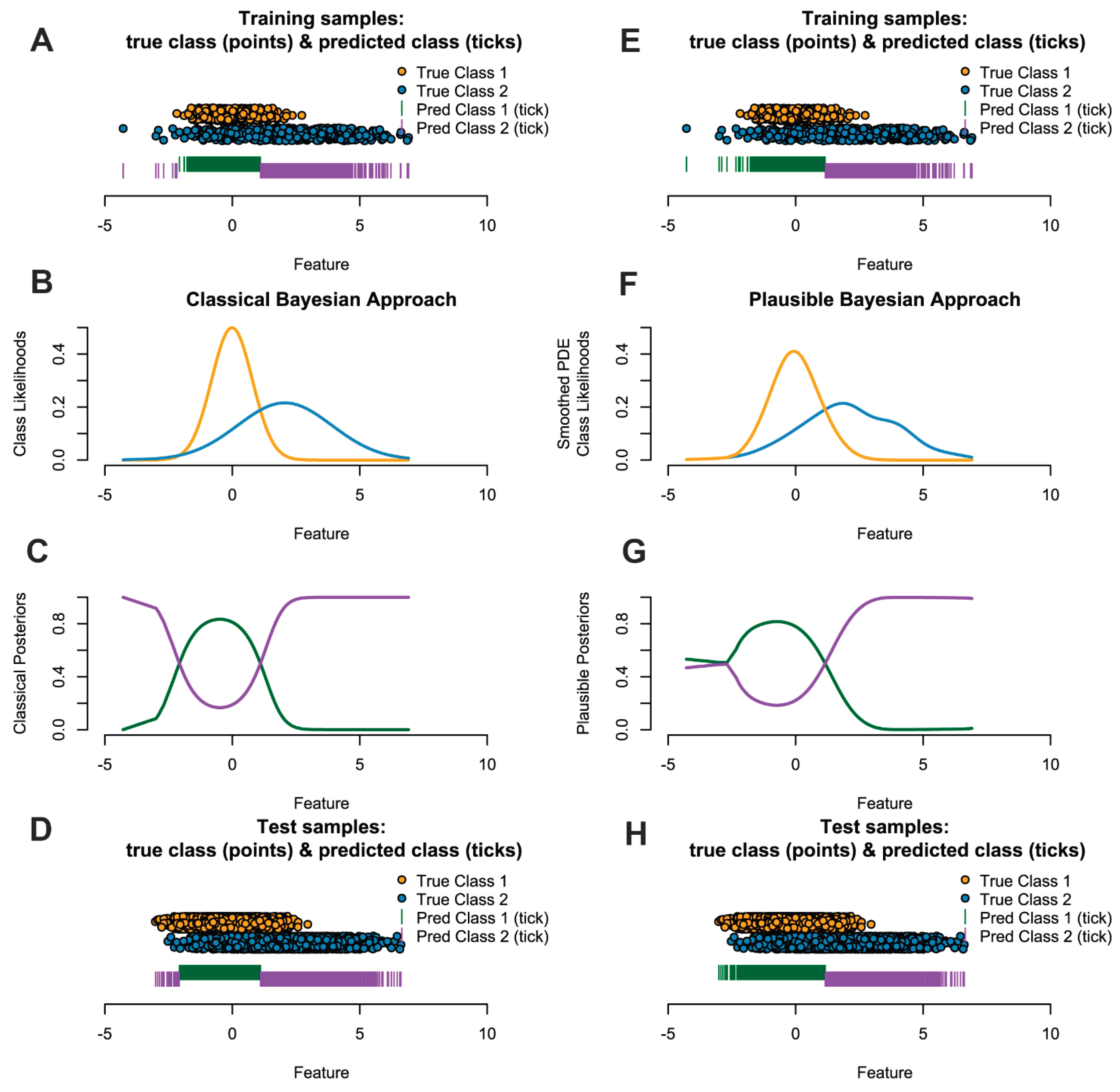
A pitfall in Bayesian theory occurs if observations with low evidence are assigned to a class with higher likelihood than another without considering that the probabilities of a probability density with higher variance decays slower than one with lower variance creating the situation that a class assignment chooses a far distant class with high variance over a closer class with smaller variance [Ultsch/Lötsch, 2022b]. An example for that would be the size of humans according to gender, where the females (Gaussian) distribution has higher variance than the males (Gaussian) distribution and the females mean is left of that of males. In that case, the classical Bayes theorem would assign a giant’s size to the class of females, since the likelihood of the males’ distribution would decay faster than that of the females. Instead, the closest mode could be chosen, if facing observations with low evidence (the giant size). As a consequence, the non-interpretable choice is to classify all giants as female. Figure 1 outlines this situation for univariate on the left side and sketches influence of the flexible approach of smoothed Pareto density estimation (PDE) in combination with plausibility correction.
Figure 1.
Left (A-D) and right (E-H) panels show results on artificial data for the classical and plausible PDE-based naïve Bayes classifier, respectively. Each panel contains four rows: N=500 sampled points with predicted labels (A, H), class-conditional densities estimated from the training data (B, F), the posterior probability P(C1∣x) computed from the fitted model (C, G), and the test set of N=5000 points with its predictions (D, H). Because class 1 (dark green) has a smaller variance, its posterior decays in both tails and the MAP rule assigns extreme observations to class 2 in C; We argue to use the smoothed PDE to estimate the class likelihoods and the concept of Ultsch & Lötsch (2022) to correct assignments in regions of very low likelihood are not plausible in F. The right panel shows that the fine structure of disributions should be accounted for in the class likelihoods (F). Without prior knowledge, applying the left model C to the test data produces misclassifications relative to the true boundary and is less interpretable in comparison to G and H.
We are proposing a new methodology for the naïve Bayes classifier overcoming these challenges and improving performance. Our approach does not make any prior assumption about density distribution, creating an algorithm free of assumptions about the data distribution. Furthermore, we dispose any parameters to be optimized [Ultsch, 2005]. We use a model of density estimation based on information theory defined by a data-driven kernel radius without intrinsic assumptions about the data that outperforms typical density estimation approaches empirically [Thrun et al., 2020]. The main contribution of our work is:
- Solution of the above-mentioned pitfall of the Bayes theorem within a Naïve Bayes classifier framework.
- Empirical benchmark showing a robust classification performance of the plausible naïve Bayes classifier using the Pareto Density Estimation (PDE).
- Visualization of the class-conditional likelihoods and posteriors to support model interpretability.
The aim of our work is to provide a classifier that can serve as a baseline. Hence, we will show that the performance of naïve Bayes is hard to associate with dependency measures and the design decisions are fluid across the degree of correlation and the choice of the correlation measure.
2. Materials and Methods
Let a classification } be a partition of a Dataset D consisting of N=|G| data points into k∈ℕ non-empty, disjoint subsets (classes) [Bock, 1974, p. 22]. Each class contains a subset of datapoints and each datapoint is assigned is a class label ∈{1,…,k} via the hypothesis function ℎ: D→{1,…,k}. The task of a classifier is to learn the mapping function h given training data and labels .
2.1. Bayes Classification
Assume a set of continuous input variables , with vector . In Bayesian classification, the prior is the initial belief (“knowledge) about class membership.
The Bayesian classifier picks the class whose posterior has the highest probability
The posterior probability captures what is known about , now that we have incorporated . The posterior probability is obtained with the Bayes Theorem
Here is the conditional probability of given class called class likelihood and the denominator is the evidence. Let H be the hypothesis space and being a MAP hypothesis, the (not necessarily i.i.d.) data set. A Bayes optimal classifier [Mitchell, 1997] is defined by
Equation 3 yields the optimal posterior probability to classify a data point in the sense that it minimizes the average probability error [Duda et al., 2001].
The general approach to Bayesian modeling is to set up the full probability model, i.e., the joint distribution of all entities in accordance with all that is known about the problem [Fukunaga/Kessell, 1971]. In praxis, given sufficient knowledge about the problem, distributions can be assumed for the and priors with hyperparameters θ that are estimated.
For the goal of this work of using a Bayesian classifier to measure a baseline of performance we make the assumption that the classification of the data point can be computed by the marginal class likelihoods with
which is called the naive assumption because it assumes i.d.d. given the classification set G. In some domains the performance of a naive bayes classifier has been shown to be comparable to neural networks and decisions trees [Mitchell, 1997]. We will show in the results that for typical datasets, even if this assumption does not hold true, an acceptable baseline performance can be computed.
Our objective is to exploit the empirical information in the training set to derive, in a fully data-driven manner and under as few assumptions as possible, an estimate of each feature’s distribution within every class , and then to evaluate classifier performance on unseen test samples. To this end, we adopt a frequentist strategy: we estimate the class-conditional densities directly from the observed data, and we compute the class priors as the relative frequencies of each in the training sample—assuming that the sample faithfully represents the underlying population. Because our decision rule is given by Equation (4), which compares unnormalized scores across classes, the global evidence term (the denominator in Bayes’ theorem) may be treated as a constant and hence omitted.
The challenge is to estimate the likelihoods given the samples of the training data. However, by using the naive assumption, the challenge of estimating the -dimensional density is simplified to estimating one-dimensional densities. In prior works, the first naive bayes classifier using density estimation was introduced as flexible bayes [John/Langley, 1995]. This work improves significantly on the task of parameter-free univariate density estimation without making implicit assumptions about the data (c.f. [Thrun et al., 2020]).
2.2. Density Estimation
The task of density estimation can be achieved in two general ways. First, parametric statistics, meaning the fitting of parametrized functions as a superposition where the fitting can be done according to some quality measure or some sort of statistical testing. The drawback here is the rich possibility of available assumptions. A default approach could be the use of Gaussian distributions fitted on the data [Michal Majka, 2024]. Second, nonparametric statistics, meaning local parametrized approximations using neighboring data around each available datapoint. It varies in the use of fixed or variable kernels (global or local estimated radius). The drawback is the complexity in tuning bandwidths for optimal kernel estimation, which is a computational hard task [Devroye/Lugosi, 2000]. A default approach to solve this problem can be a Gaussian kernel where the bandwidth is selected according to the Silverman’s rule of thumb [Bernard W Silverman, 1998].
In this work, we want to solve the density estimation with the data-driven approach called Pareto Density Estimation (PDE) taken from [Ultsch, 2005]. In this way, any prior model assumption is dropped. The PDE is a nonparametric estimation method with variable kernel radius. For each available datapoint in the dataset, the PDE estimates a radius for estimating the density at this point. It uses a rule from information theory: The PDE maximizes the information content (reward) while minimizing the hypersphere radius (effort). Since this rule is historically known as Pareto rule (or 80-20-rule, reward/effort-trade-off), the method is called Pareto Density Estimation.
2.3. Pareto Density Estimation
Let a subset of data points have a relative size is . If there is an equal probability that an arbitrary point x is observed, then content is . The optimal set size is the Euclidean distance of S from the ideal point, which is the empty set with 100% information [Ultsch, 2005]. The unrealized potential is . Minimizing the yields the optimal set size . This set retrieves 88% of the maximum information [Ultsch, 2005]. For the purpose of univariate density estimation, the computation of the univariate Euclidean distance is required. Under the MMI assumption the squared Euclidian distances are χ-quadrat distributed [Ultsch, 2003] leading to
where is the Chi-square cumulative distribution function for d degrees of freedom [Ultsch, 2005]. The pareto Radius is approximated by for .
The PDE is an adaptive technique for estimating the density at a datapoint following the Pareto rule (80-20-rule). The PDE is maximizing the information content using a minimum neighborhood size. It is well suited to estimating univariate feature distributions from sufficiently large samples and to highlighting non-normal characteristics (multimodality, skew, clipped ranges) that standard, default-parameter density estimators often miss. In an empirical study, Thrun et al. (2020) demonstrate that PDE visualizations (mirrored-density plots, short MD plot) more faithfully reveal fine-scale distributional features than standard visualization defaults (histograms, violin plots, and bean plots) when evaluated across multiple density-estimation approaches. Accordingly, PDE frequently yields superior empirical performance relative to commonly used, default-parameter density estimators. [Thrun et al., 2020].
Given the pareto radius R, the raw PDE can be estimated as discrete function solely at given kernel points with
where 1 is an indicator function that is 1 if the condition holds and 0 otherwise, A normalizes , and a quantized function that is proportional to the number of samples falling within the interval [-R, +R].
For the mirrored-density (MD) plots used in Thrun et al. (2020), we previously applied piecewise-linear interpolation of the discrete PDE to fill gaps between kernel grid points and obtain a continuous visual approximation of a feature’s pdf While linear interpolation produces a visually faithful representation and is adequate for exploratory plots as it preserves continuity and is trivial to compute, it inherits the small-scale irregularities of the underlying discrete PDE estimate. If linearly interpolated densities are used directly as class-conditional likelihoods in Bayes’ theorem, that high-frequency noise propagates into the posteriors and can produce unstable or incorrect classifications.
Accordingly, in this work we therefore proceed as follows. After obtaining the raw and discrete conditional PDE ,we replace linear interpolation by several smoothing steps in the next section that produce a class likelihood which (i) preserves genuine distributional structure (modes, skewness, tails) and (ii) suppresses spurious high-frequency fluctuations that would destabilize posterior estimates.
2.4. Smoothed Pareto Density Estimation
Although the PDE of class likelihoods captures the overall shape of the distribution, it can be somewhat rough or piecewise-constant due to the uniform kernel and finite sampling. This is disadvantageous as irregular or noisy estimates yield fluctuating posteriors and unstable decisions. Therefore, smoothing the class likelihoods acts as a form of regularization: it suppresses sample-level noise and prevents high-frequency fluctuations like erratic spikes or dips in the likelihoods that lead to brittle posterior assignments. Balancing the fidelity to the PDE’s “true” features with removal of artificial high-frequency components results in more accurate approximations of the true underlying distributions leading to more reliable posterior estimates because they are less influenced by random sample noise.
For smoothing we exploit the insight, that the kernel estimate is a convolution of the data with the kernel by using fast Fourier transforms [Bernard W Silverman, 1998] p.61. To produce a smooth continuous density estimate, we convolve the PDE output with a Gaussian kernel using the Pareto radius as the bandwidth. Hence, the Gaussian smoothing kernel is defined as
where R is the pareto radius. We use the Fast Fourier Transform (FFT), leveraging the convolution theorem in order to implement this convolution efficiently as follows.
First, we evaluate the Gaussian kernel on the same grid as the PDE in which is the number of grid points. Let be the grid spacing, then the Gaussian kernel vector
yields a normalized kernel vector aligned with the PDE grid and we use the mean of adjacent differences to avoid numerical instabilities in spacing.
To perform a linear convolution without wrap-around artifacts, we zero-pad both the density and kernel vectors before FFT [Blackman/Tukey, 1958] (part1, p.260ff). We choose the padding length as the next power of two. This length ensures that circular convolution via FFT corresponds to the linear convolution of the original sequences, and using a power of two leverages FFT efficiency [Jones/Lotwick, 1984]. We create padded vectors (the with zero-pad) and ( with zeros zero-pad), each of length L. This padding avoids overlap of the signal with itself during convolution.
Next, we compute the FFT of both padded vectors, multiply them element-wise in the frequency domain, and then apply the inverse FFT. By the convolution theorem, the inverse FFT of the product
yields the linear convolution on the padded length. We divide by L in equation 9 when taking the inverse FFT, as per normalization convention.
The central elements correspond to the convolved density over the original grid. This middle segment is the smoothed density vector , aligned with the original kernel grid. The approach is motivated by the idea of [Bernhard W Silverman, 1982].
Finally, the montone Hermite spline approximation of [Fritsch/Carlson, 1980] yields the likelihood function . and allows for a functional fast computation of new points.
In sum, the empirical class PDE in a dimension can be rough due to the data being noisy. If used for visualization task, the roughness was inconsequential [Thrun et al., 2020]. In order to not influence the posteriors by data noise, we propose as a solution a combination of filtering by convolution (c.f. [Scott, 2015]) and monotonous spline approximation (c.f.[Bernard W Silverman, 1984]) yielding .
2.5. Plausible Naïve Bayes classification
Ultsch and Lötsch showed that misclassification can occur when only low evidence is used in the Bayes’ theorem, i.e., the cases lie below a certain threshold ε. They define cases below ε as uncertain and provide two solutions [Ultsch/Lötsch, 2022b]: reasonable Bayes (i.e. suspending a decision) and plausible Bayes (a correction of equation 4). To derive ε they propose the use of the computed ABC-analysis [Ultsch/Lötsch, 2015]. The algorithm allows to compute precise thresholds that partition a dataset into interpretable subsets.
Closely related to the Lorenz curve, the ABC curve graphically represents the cumulative distribution function. Using this curve, the algorithm determines optimal cutoffs by leveraging the distributional properties of the data. Positive-valued data are divided into three disjoint subsets: A (the most profitable or largest values, representing the 'important few'), B (values where yield matches effort), and C (the least profitable or smallest values, representing the 'trivial many').
Let be a set of n observations which for the purpose of defining the plausible Naïve Bayes likelihoods in dimension are indexed in non-decreasing order in the respective dimension, i.e., , let , the is defined by [Gastwirth, 1971] as
For all other p in [0,1] with p ≠ pi, L(p) is calculated using some linear, spline or other suitable interpolations on [Gastwirth/Glauberman, 1976].
Let L(p) be the Lorenz curve in equation 11 then the ABC curve is formally defined as
Then the break-even point satisfies and the submarginal point is located by minimizing the distance from the ABC curve to the maximal-yield point at (1,1) after passing the break-even point with . The break-even point yields the BC limit, and, hence, the threshold ε with
Equation 12 defines the BC-Limit.
Inspired by their idea, we reformulate the computation of epsilon from posterior to joint likelihood as follows. An observation is considered uncertain in featurewhenever the joint likelihood every class falls below the confidence threshold ε, i.e.
where denotes the marginal of the distribution in dimension . We will apply the threshold ε to identify low-evidence regions where the plausibility correction (Eq. 15) may be considered. Such uncertain cases might be classified against human intuition to a class with a probability density center quite far away despite closer available class centers [Ultsch/Lötsch, 2022b]. Then a “reasonable” assignment might be to assign the case to the class whose probability centroid is closest which can be calculated using Voronoi cells for d>1. For the one-dimensional case they propose the closest mode could be determined for classifying such cases.
We estimate the univariate location of each class likelihood’s mode on a per-feature basis using the half-sample mode [Bickel/Frühwirth, 2006]. For small sample sizes (n < 100) we use the estimator recommended by [Ekblom, 1972]. As a safeguard mechanism, estimated modes are only considered for resolving uncertain cases if they as well-separated, i.e., have a distance from each other of at least the 10th percentile within the training data
This mechanism is motivated by the potential presence of inaccurately estimated modes or overlapping (non-separable) classes.
When the class likelihood for an observation x is uncertain in feature (Eq. 13 holds true) and there is a class whose mode is well-separated from the highest-likelihood class (Eq. 14), we perform a conservative, local two-class correction of that feature class likelihoods as follows:
Let be the index of the uncorrected class likelihood with the largest value and the index of the class likelihood with closest mode to for which equation (14) hold true for and .
Then we update the two involved class likelihoods by replacing the values of the class likelihood with the (former) top class likelihood . In addition, the operation subtracts δ from the prior top likelihood and adds δ to the runner-up , the relative advantage of the runner-up versus the former top increases by 2δ, which is sufficient to resolve many marginal posterior ties or implausibilities (as shown in the example in figure 1) while remaining conservative. All other class likelihoods for this feature remain in Eq. 15 unchanged:
Equation 4 is then used with the locally corrected class likelihoods . Note that as the correction vanishes and the method reduces to the reasonable-Bayes rule; the transfer introduces a conservative “plausible-Bayes” adjustment, with controlling the strength of the plausibility correction.
2.6. Practical Considerations
In order to avoid numerical overflow, equation (4) with uncorrected or the with the locally corrected class likelihoods can be computed in log scale
to select the label of the class that with the highest probability.
In praxis, before this function can be computed, it must be determined if there are enough samples to yield a proper PDE. Based on empirical benchmarks [Thrun et al., 2020], if there are more than 50 samples and at least 12 uniquely defined samples, then then can be estimated, otherwise the estimations might deviate. In case of too few samples, the density estimation defaults to simple histogram binning with bin width defined by Scott`s rule [Keating/Scott, 1999].
Let be a small constant, then to ensure numerical stability in equation 16, the likelihoods are clipped to the range of . The reason is, that density after smoothing may result in values slightly below zero due to the convolution (c.f. [Bernard W Silverman, 1998]). In addition, density estimation can have spikes above 1. Moreover, we ensure numerical safety if we clip the corrected likelihoods to be non-negative after applying equation (15).
There is also a possibility that equation 4 may not allow a decision as two or more posteriors equal each other after the priors are considered. In such a case, the class assignment is randomly decided.
Equation (15) foundation is the assumption that modes can be estimated correctly in the data per class which could fail in praxis. As a safeguard, we provide for the user the following option. We compute the classification assignments as defined in Equation (4), transformed according to Equation (16), and likewise without correction , both using the training data.
Assuming the priors are not excessively imbalanced, we evaluate the Shannon entropy of each classification result and choose the configuration that yields the highest entropy. The Shannon entropy H of with priors for is defined as
with the normalization factor .
A higher entropy indicates a potentially more informative classification.
Finally, due to the assumption leading to equation (4) and subsequent equations, we provide a scalable multicore implementation of the plausible bayes classifier by computing every feature separately proceeding as follows: For each feature dimension we estimate a single Pareto radius independent of class as defined in Equation (5) rather than separately for each feature-class combination. Empirical evaluations indicate that this approximation is sufficiently accurate for practical applications. For each class in each dimension we compute the class-wise PDE on an evenly spaced kernel grid to compute the raw conditional PDE covering the range of the data. Then, we compute the smoothed likelihood functions per feature dimension from the discrete conditional PDE . We call this approach the Plausible Pareto Density Estimation based flexible Naïve Bayes classifier (PDENB).
2.7. Interpretability of PDENB
The one-dimensional density estimation required for the Naïve Bayes Classifier to compute the class-conditional likelihood of a feature as one of three parts of the Bayes theorem yielding the final Posterior. This class-conditional likelihood allows a two-dimensional visualization as a line plot for a single feature. The plot gives insight into the class-wise distribution of the feature. Scaling the likelihoods with the weight of the prior obtained from the frequentist approach [Duda et al., 2001] yields the correct probabilistic proportions between the class-conditional likelihoods which can be represented by different colors. Rotating the plots by 90 degrees and mirroring similar than for violin and mirrored density plots [Thrun et al., 2020] allows the lineup of the likelihoods for multiple features at once. Such visualization allows interpretation based on the class-wise distribution of features. Most likely, the colored class conditional likelihoods are overlapping and non-separable by solely one feature. However, in case of a high performing Naïve Bayes Classifier, overlaps do not indicate non-separability, but rather first of all a class tendency for each feature and second the existence of certain combinations and a disqualifier for other combinations in question. These visual implications can be the starting point for a domain expert to find relations between features and classes resulting in explanations.
Additionally, we provide a visualization of one class versus all decision boundaries in 2D as follows. Given a two-dimensional slice , the Voronoi cell associated with a point g is the region of the plane consisting of all points that are closer to g than to any other point v in the slice is defined by
That is, contains all points such that the Euclidean distance from any y to g is less than or equal to the distance to any other v. Each Voronoi cell according to the binned posterior probability , thereby mapping regions of the plane to their inferred class likelihoods by colors. The binning can be either performed equally sized using Scotts rule as bin width [Keating/Scott, 1999] or less efficiently by the DDCAL clustering algorithm [Lux/Rinderle-Ma, 2023]. The user can visualize the set of slices of interest. This approach is motivated by human pattern recognition and subsequent disease classification of identified patterns in two-dimensional slices of data [Shapiro, 2005] that apparently is sufficient for a large variety of multivariate data distributions.
2.8. Benchmark Datasets and Conventional Naïve Bayes Algorithms
For the benchmark we selected 14 datasets: 13 from the UCI repository and a fourteenth dataset (“Cell populations”) containing manually identified cell populations [Plank et al., 2021]. Full dataset descriptions of the UCI datasets, attribute definitions and links to original sources are available on the repository pages for each dataset [Dua/Graff, 2019], for example or example, Iris: https://archive.ics.uci.edu/ml/datasets/iris). The Cell populations dataset is an extended version of the data used by Plank, Dorn & Krause (2021); the set of populations provided here is larger than in that publication because the authors labeled populations at finer granularity. A detailed description of the cell populations dataset is given in Plank et al. (2021).
The datasets were preprocessed priorly using methods rotation [Pearson, 1901; Hotelling, 1933] drawing [Karlis et al., 2003; Harmeling et al., 2004] as implemented in “ProjectionBasedClustering” available on CRAN [Thrun/Ultsch, 2020]. In it should be noted that although to the cell populations the signed log transformation for better interpretability was applied, no Euclidean optimized variance scaling was used[Ultsch/Lötsch, 2022a]. Thereafter, correlations of features were computed. Important properties and meta information, and correlations of the processed datasets are stated in table 1. The measure of correlation depends on the choice of algorithm. Here, the Pearson, Spearman’s rank, Kendall’s rank and the Xi correlation coefficient [Chatterjee, 2021] are summarized using the minimum and maximum value to characterize the correlations of the datasets. The values of the Pearson and Spearman correlation coefficient tend to be higher than the Xi correlation coefficient by around 0.3. Similarly, Kendall’s Tau values tend to be higher than the Xi correlation coefficients but not as high as the Pearson’s or Spearman’s correlation coefficients. Important attributes are the number of classes, the distribution of cases per class to judge class imbalance and various dependency measures related to the independent feature assumption of the naïve Bayes classifier are presented in table 1.
The performance is evaluated for the Plausible Pareto Density Estimation based flexible Naïve Bayes classifier (PDENB) in comparison to a Gaussian naïve Bayes classifier (GNB) and a nonparametric naïve bayes classifier (NPNB) from the R package “naivebayes” available on CRAN [Michal Majka, 2024]), a fast implementation of k-nearest neighbor classifier (kNN) from the R package “FNN” available on CRAN [Li, 2024]), a Gaussian naïve Bayes from the python package “sklearn” [Buitinck et al., 2011], a Gaussian and non-parametric naïve Bayes approach from the R package “klaR” available on CRAN [Roever et al., 2023], and last but not least a Gaussian naïve Bayes from the R package “e1071” available on CRAN [Meyer et al., 2024]. The algorithms for the naïve bayes methods were applied in their default settings differencing between “Gaussian” and “nonparametric” versions, while the parameter k for the kNN classifier is set to 7.
3. Results
The first subsection presents the classification performance in detail. Subsection 2 presents visualizations that support model interpretability and subsection 3 provides an application.
3.1. Classification Performance
Table 1 presents the benchmark across 14 datasets. Following the work of [Breiman, 2001; Hall/Frank, 2008] small datasets with up to 10.000 samples are evaluated with 100 times repeated hold-out set using the 80-20 rule. Datasets with higher sample sizes are evaluated once with a hold-out set (80-20-rule) and 100 mean samples are obtained with a resampling technique. The performance in each trial is evaluated with the Matthews correlation coefficient (MCC) [Chicco/Jurman, 2020] [Chicco et al., 2021]. The results are summarized in tables using the means of the 100 evaluated trials in table 2. The distributions are shown using Mirrored-Density-plots (MD-plots) in the supplementary A, see Figure 1-14. “NA” values indicate a failure of the classification algorithm. For the case of MiceProtein, several classifiers failed due to missing values in the dataset. The remaining cases of “NA” values can be observed for klaRGNB: for the datasets Dermatology, Spam and Covertype, errors due to the estimation of variance are reported. The reason for that are the discrete features within the datasets, which cannot be estimated properly by the implementation. The results show that high correlation values are not necessarily an indicator for low performance of the naïve bayes classifiers (compare Table 1 to Table 2).
We find that no single algorithm consistently outperforms all others, in line with the no-free-lunch theorem (Wolpert, 1996). However, it is still possible to rank algorithms based on their mean performance, considering their best-performing variants across trials, while allowing for ties. To this end, we apply the permutation test [Good, 2013] pairwise to each evaluation (see table B1 in the supplementary). This statistical test determines whether performance differences are significant or not, enabling rankings with possible ties. From these results, we obtain a ranking of classifiers for all datasets (see table B2). Finally, we compute the mean of these ranks to derive an overall score for each algorithm, presented in Table 3.
3.2. Interpretable Naïve Bayes Classifier
One advantage of the PDE-based, flexible naïve Bayes classifier is that it relies on one-dimensional density estimates, which we use to visualize class-dependent fine structure of distributions for each feature. Inspecting all class-conditional likelihoods for a feature at once can reveal interesting relations or patterns when the number of dimensions allows such an overview; otherwise, a targeted feature selection is required. Figure 2, Figure 3, Figure 4, Figure 5, Figure 6, Figure 7 and Figure 8 show class-conditional likelihoods for four representative datasets: Satellite, Iris, Penguin, and the Cell populations dataset on the training data for one arbitrary cross-validation trial.
Figure 2.
A The figure shows the class-conditional PDE likelihoods for the first two feature of dataset “Cell populations”. The colors depict different classes and are mapped to the cell populations. The legend presents the name of the cell population classes and applies also for the following sub figures B-D. B The figure shows the class-conditional PDE likelihoods for the next four features dataset “Cell populations”. The colors depict different classes as mapped to the legend in figure 2. The values are transformed to the signed log scale as provided in the package “DataVisualizations” on CRAN [Thrun/Ultsch, 2018]. C The figure shows the class-conditional PDE likelihoods for the next four features of dataset “Cell populations”. The colors depict different classes as mapped to the legend in figure 2. The values are transformed to the signed log scale as provided in the package “DataVisualizations” on CRAN [Thrun/Ultsch, 2018]. D The figure shows the class-conditional PDE likelihoods for the last three features of the “Cell populations” datasets. For comparison FS_TOF in a different range is shown again. The colors depict different classes as mapped to the legend in figure 2. The values are transformed to the signed log scale as provided in the package “DataVisualizations” on CRAN [Thrun/Ultsch, 2018].
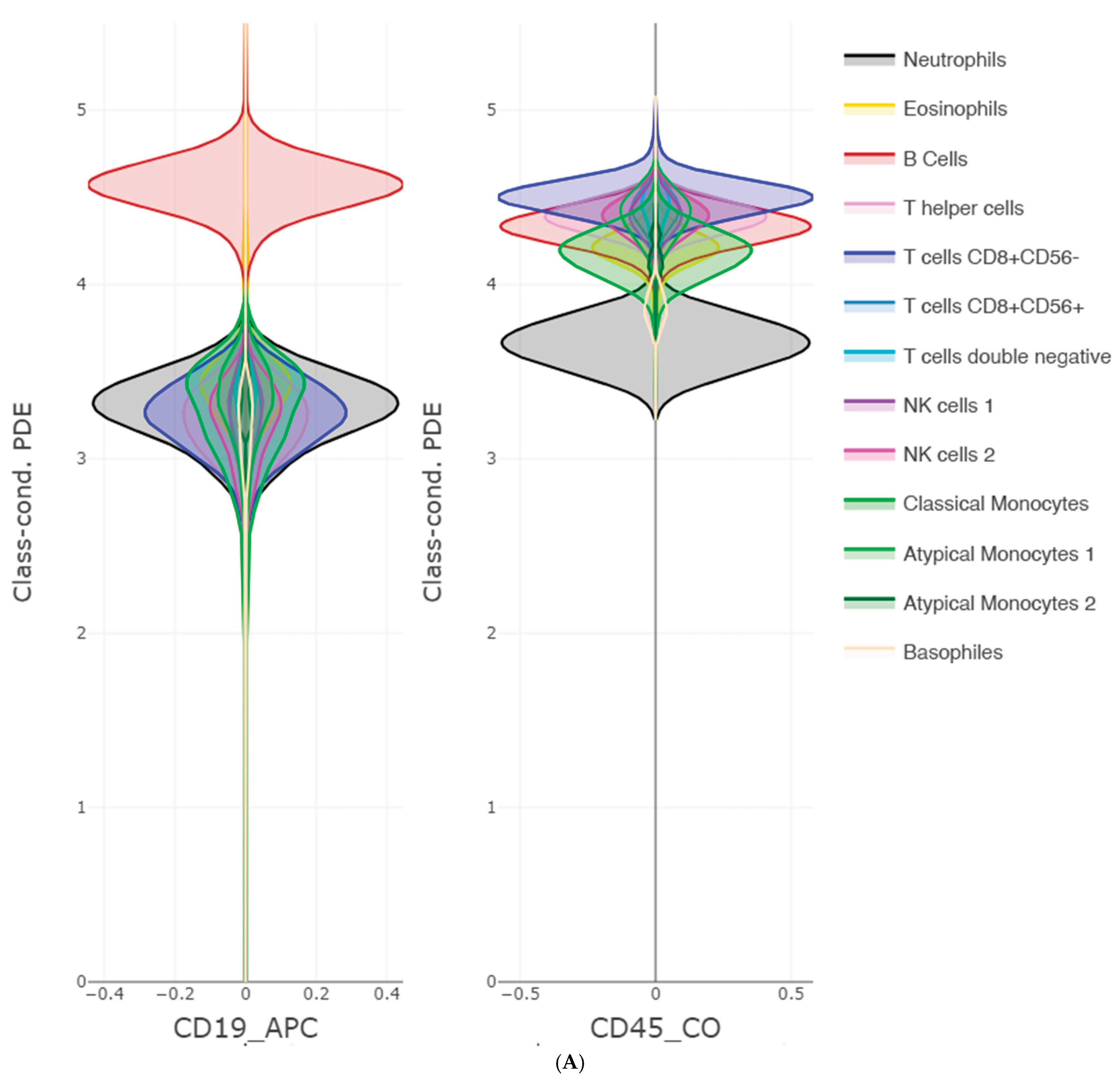
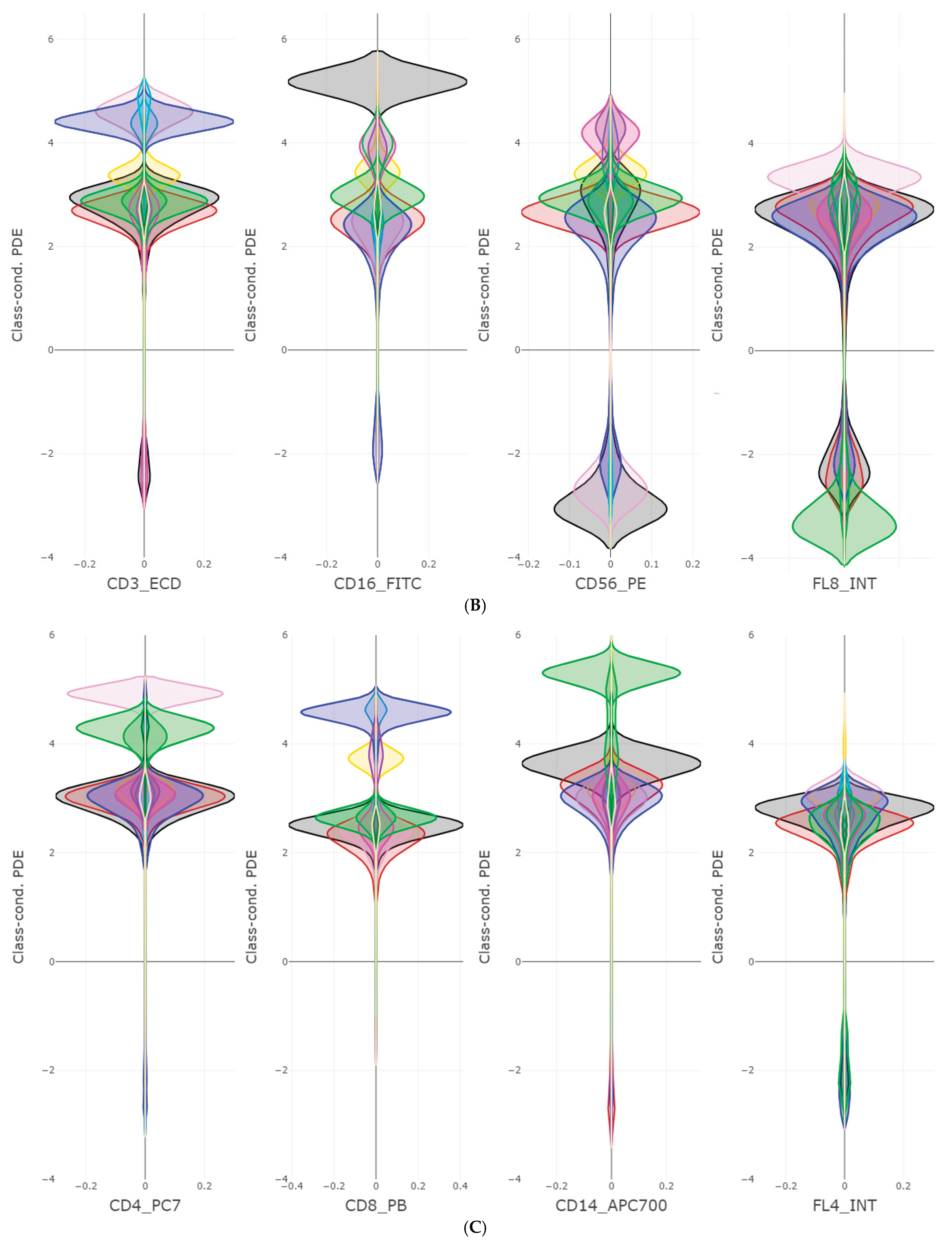
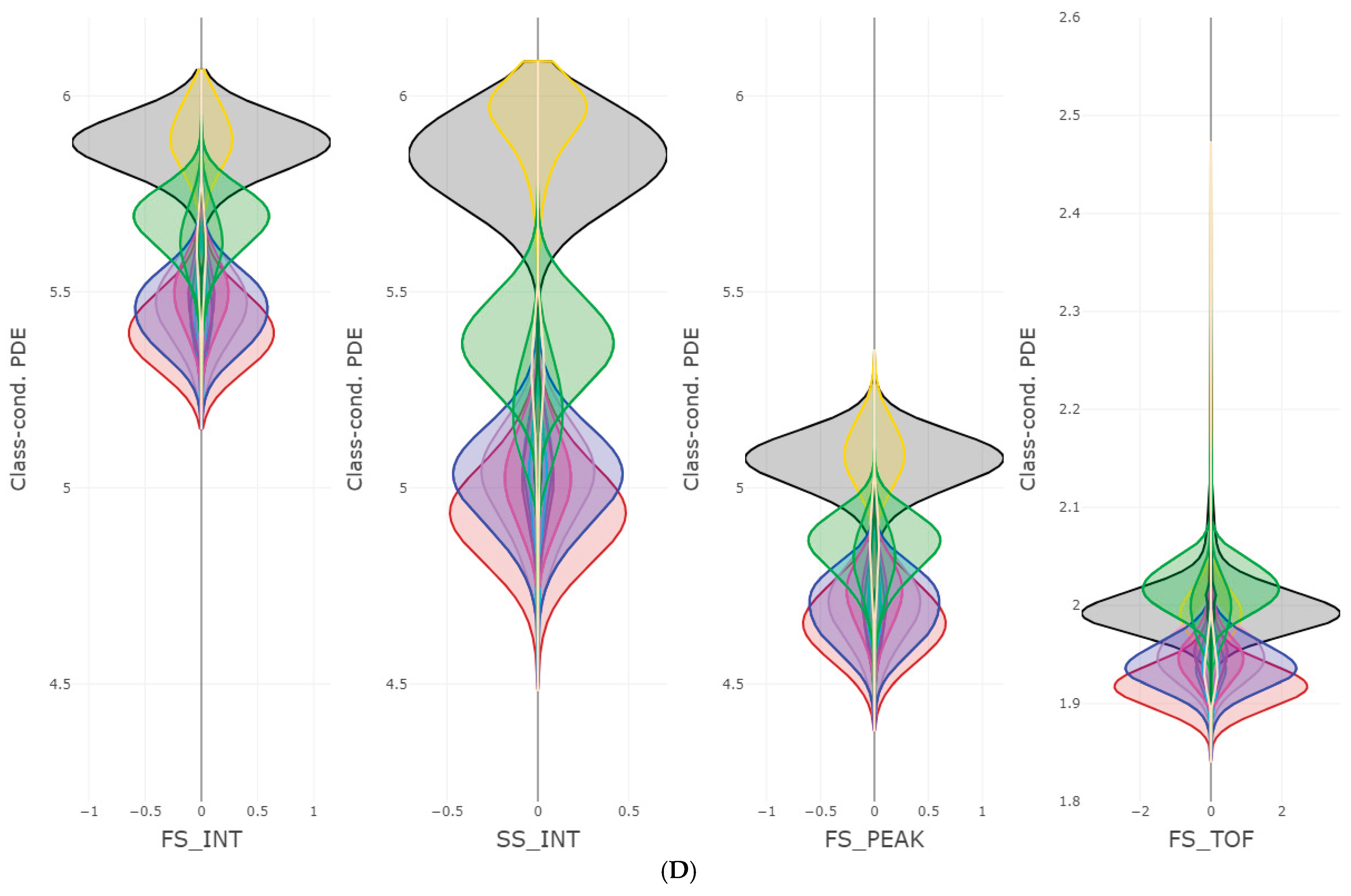
Figure 3.
The figure visualizes the fine distribution structure of the class-conditional PDE likelihoods for a selected subset of features from the Satellite dataset, highlighting differences in skewness, tails and multimodality across classes. The colors depict different classes. Each feature contains varying non-classic distributions with different characteristics such as long and fat tails, multimodal and skewed distributions which can be assessed visually.
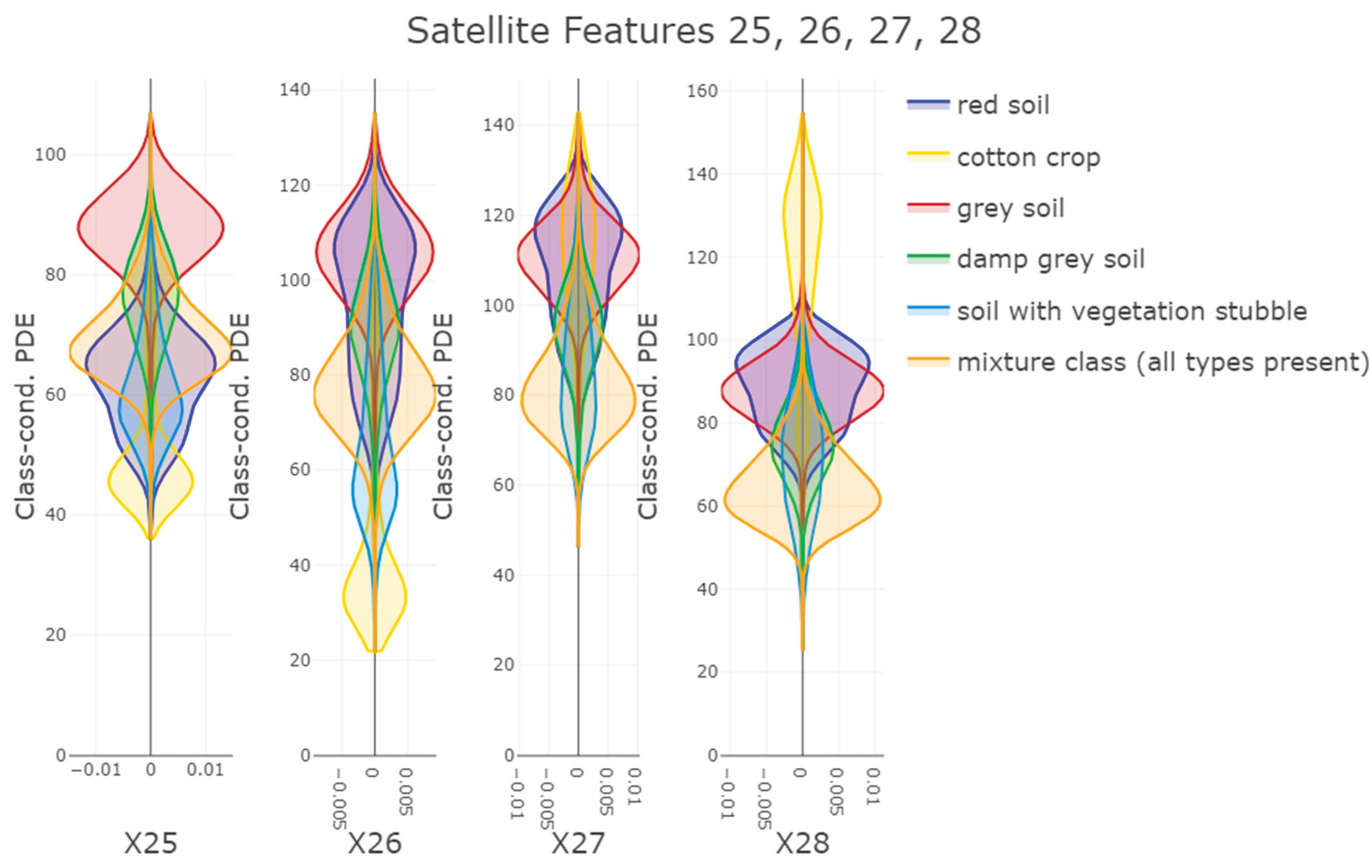
Figure 4.
The figure shows the class-conditional PDE likelihoods for the 4 features of dataset “Iris”. The colors depict different classes.
Figure 4.
The figure shows the class-conditional PDE likelihoods for the 4 features of dataset “Iris”. The colors depict different classes.
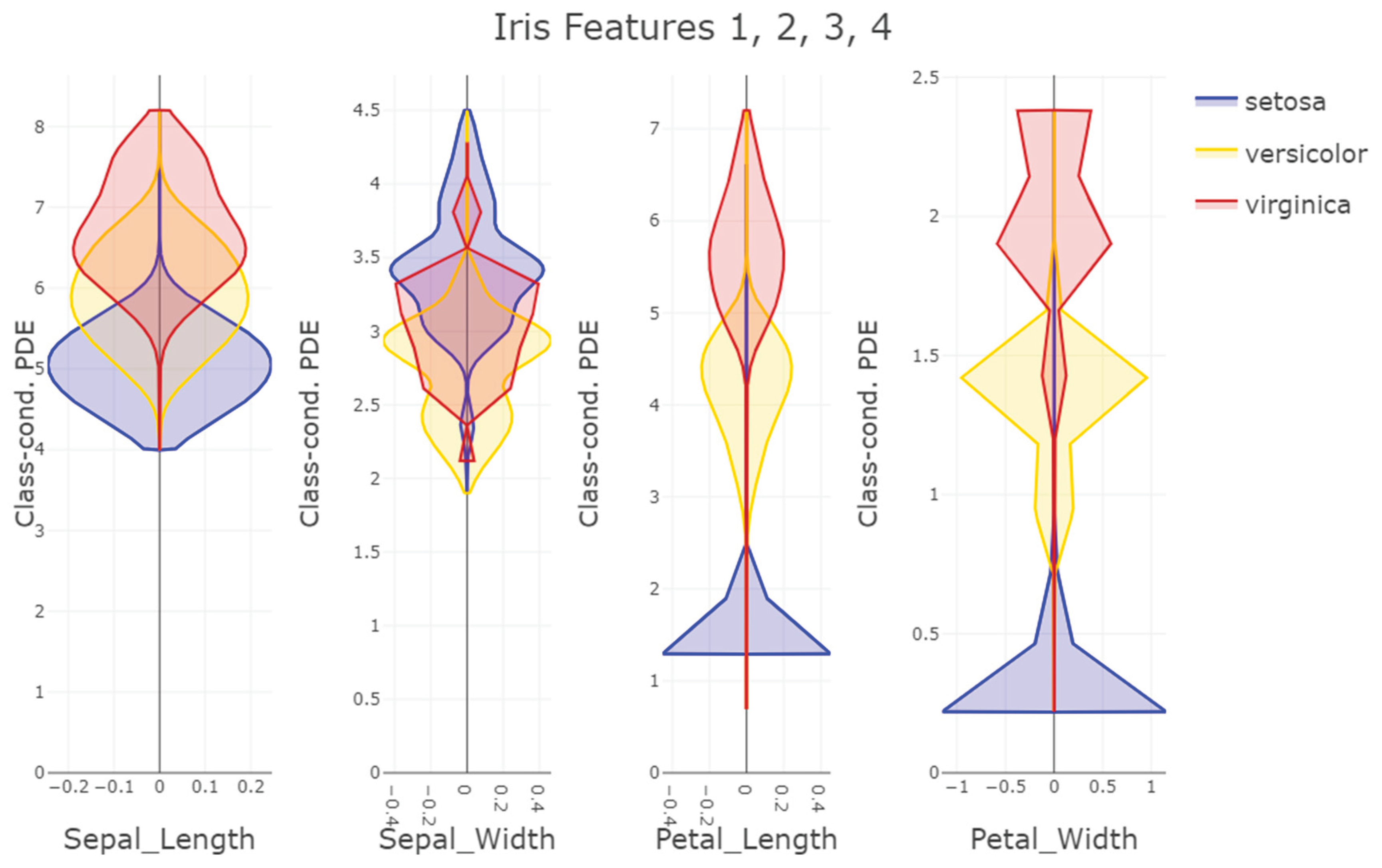
Figure 5.
The figure shows the class-conditional PDE likelihoods for the 4 features of dataset “Penguins” obtained by an ICA transformation. The colors depict different classes. Features C1–C4 were derived by applying independent component analysis (ICA) to the original variables[Comon, 1992]. Hence, the resulting components are used as rotated features for downstream analysis [Thrun, 2018].
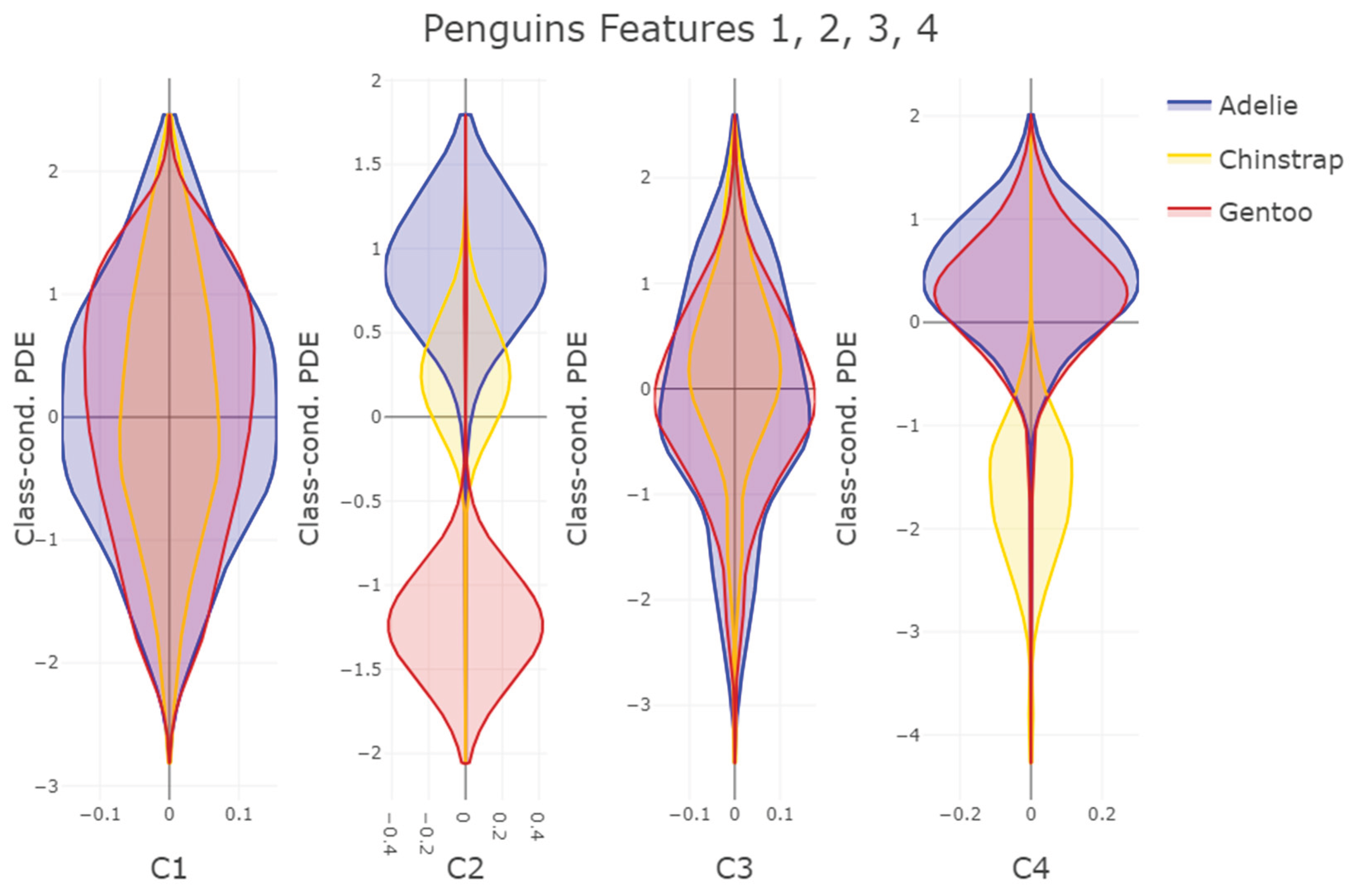
Figure 6.
The figure shows a customized 2D Voronoi tessellation based on the two ICA components C2 and C4 from dataset Penguins. The posterior for the three classes Adelie Gentoo and Chinstrap are highlighted form left to right. A compact area consisting mainly of dark red color can be detected, indicating a specific location of high posterior values for each class in the relationship between the two features. See Figure 5 for comparison to class likelihoods.
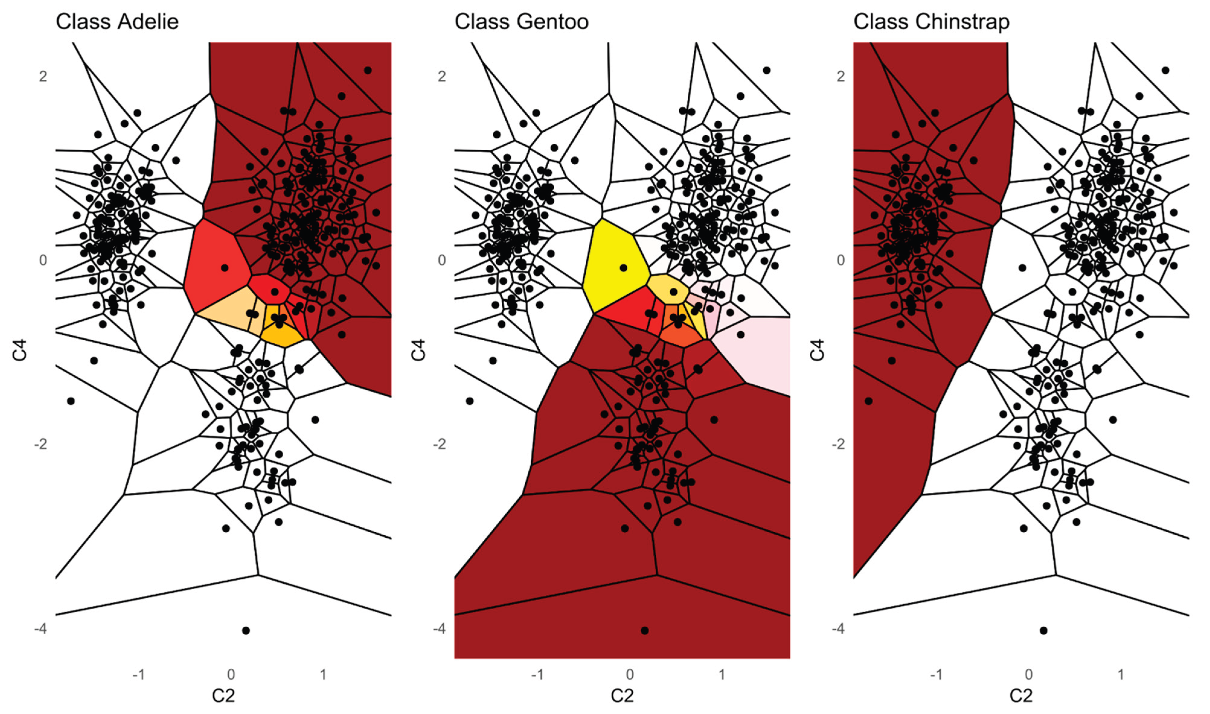
Figure 7.
The figure shows a customized 2D Voronoi tessellation based on the two features CD16_FITC and CD14_APC700 from dataset Cell populations. The posterior for the class of atypical monocytes 1 is highlighted. A compact area consisting mainly of dark red color can be detected, indicating a specific location of high posterior values for this class in the relationship between the two features. Both features are typically used to detect atypical monocytes in FlowCytometry.
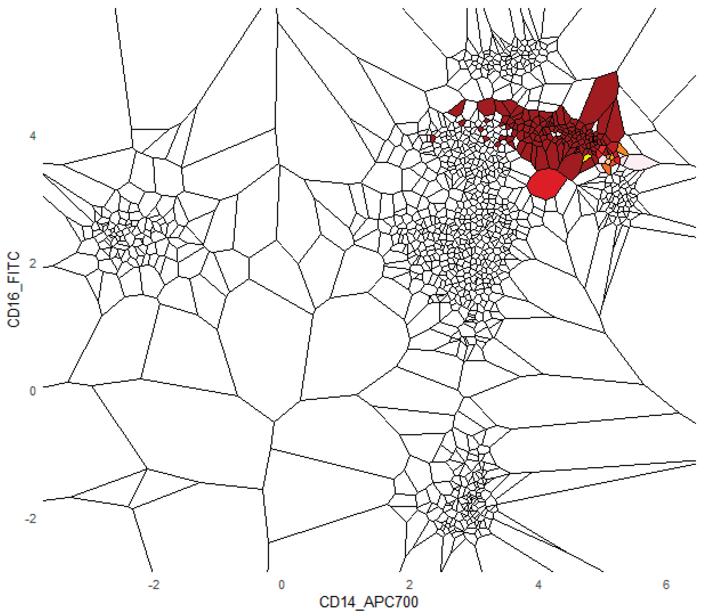
Figure 8.
The figure shows a customized 2D Voronoi tessellation based on the two features CD16_FITC and CD14_APC700 from dataset Cell populations. The posterior for class of classical monocytes is highlighted. A compact area consisting mainly of dark red color can be detected, indicating a specific location of high posterior values for class 10 in the relationship between the two features. Both features are typically used to detect classical monocyte cells in FlowCytometry.
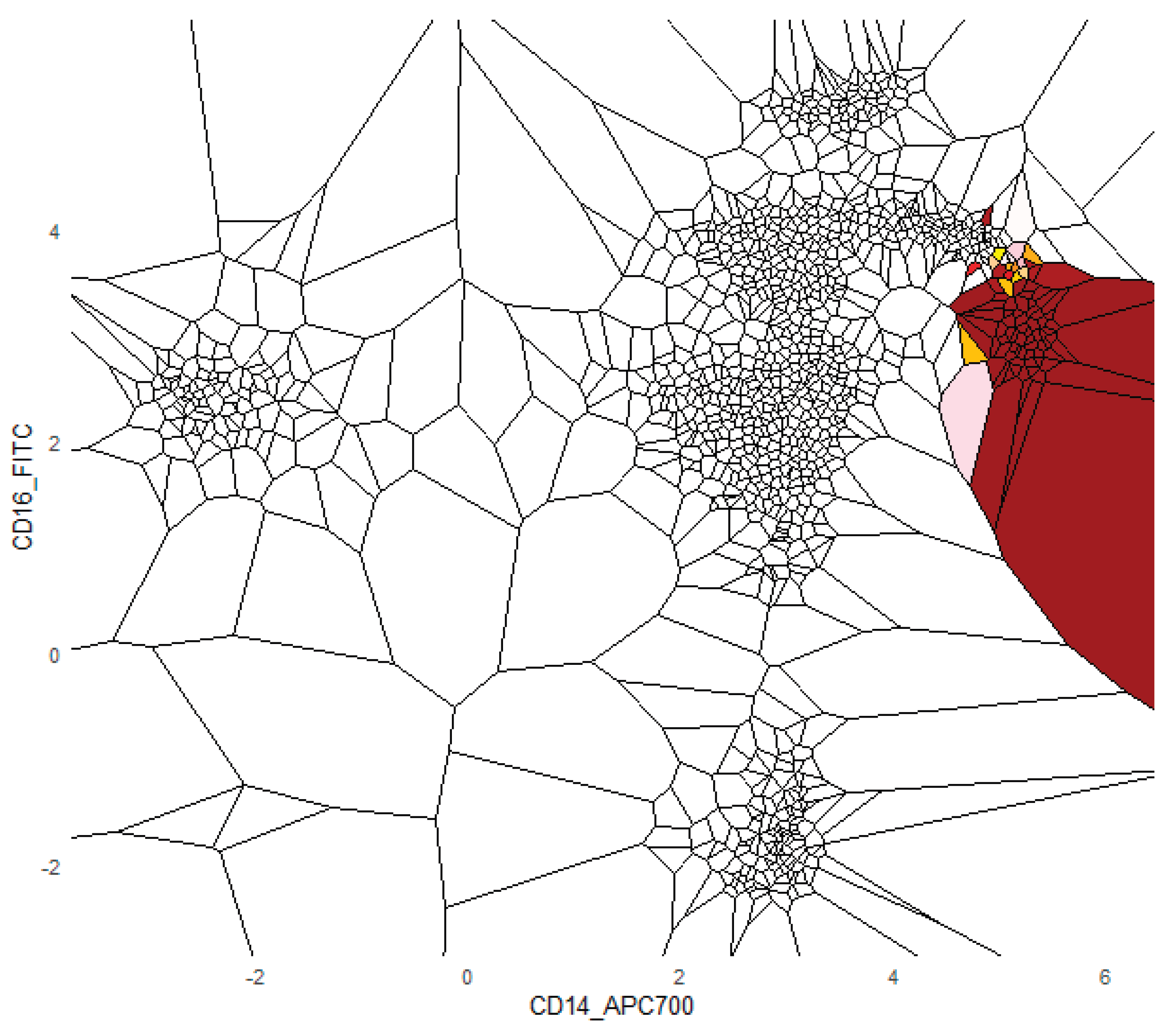
Figure 2 A-D presents the features of the annotated biological populations in the Flowcytometry dataset called Cell populations. Normally, the cells populations were manually distinguished in sequential two-dimensional dot plots. In Figure 2 A, CD45 is a pan-leukocyte antigen whose fluorescence intensity separates broad white-blood-cell compartments (lymphocytes, monocytes, granulocytes) together with side scatter and help distinguish hematopoietic from non-hematopoietic events. Within the lymphocytes CD19 is a B-lineage surface marker used to identify and quantify B cells. In Figure 2B, CD3 separates T-cells, and NK-cells can be separated because they are CD3 negative and positive for CD16 and/or CD56. FS_INT (forward-scatter integral) is a proxy for cell size and SS_INT (side scatter intergral) for granularity in Figure 2D.
Figures B–C depict two features labeled FL4_INT and FL8_INT. These channels correspond to detectors that did not match any used fluorochrome and therefore primarily record detector noise and light spillover of other detectors, see [Novo, 2022] for details. It is clearly visible that no class is distinguishable in FL4_INT in comparison to “CD16_FITC”and “CD4_PC7”. In FL8_INT, we have a spillover effect from another detector (possibly “CD14_APC700”) to FL8_INT allowing to distinguish the red class. Without medical knowledge, FL4_INT would be disregarded based on Figure C and FL8_INT would be questioned because it only distinguishes the green class (Monocytes) with negative log light measures based on Figure B which could be a light spillover of CD14 presented Figure 2 B. Based on Figure 2D, for the classification task it seems like FS_Int and FS_PEAK contain the same information w.r.t. class likelihoods with aligns with domain knowledge.
Figure 3 presents class-conditional likelihoods for the Satellite dataset and motivates the need for an assumption-free distribution estimator. The plot illustrates a variety of distributional shapes across classes and features: for example, the “mixture” class in feature 26 is skewed, the “grey soil” class exhibits increased kurtosis, and the “cotton crop” class shows long tails in several features.
Figure 4 shows the well-known Iris dataset, where clear per-class tendencies are evident; the strong performance of naïve Bayes in this example illustrates how informative one-dimensional patterns can be for classification.
Figure 5 displays the Penguin dataset: although class tendencies are visible, substantial class overlap is present. The good performance of naïve Bayes here implies that separability is achieved by combining the information of feature C2 with C4 after the ICA rotation is applied and Features C1 and C3 could be disregared
Across the visualized datasets PDENB achieved excellent performance (MCC ≥ 0.95). The per-feature PDE visualizations frequently reveal regions of class overlap at the single-feature level—not as a shortcoming, but as an exploratory strength: these plots make the limits of one-dimensional separation explicit and point to which features are complementary. By inspecting class-conditional shapes (modes, tails, skewness) across features we can identify feature combinations that produce clear separation in higher dimensions, guide feature selection, and maybe even generate meaningful explanations for the classifier’s decisions.
See Figure 6 for comparison to posteriors.Another take on visualizing patterns detected by the naïve bayes classifier would be to visualize the posterior computed in high dimensions in a two-dimensional plot. An informative plot in two dimensions can be derived from a 2D scatter plot. Given the two-dimensional coordinates, a Voronoi tessellation can be used to partition the area defined by the coordinates, as it is done in Figure 6, Figure 7, Figure 8 and Figure 9 for the training data. This representation allows a coloration of decision areas based on the posterior. High posterior values are colored as dark red, zero values as white and intermediate values as a gradient in between the range of these two colors with yellow as color for values in the middle. Within the 2D Voronoi visualization of the posterior decision boundaries, the recognition of a single compact area with high posterior values for a certain class suggests a decision pattern. For example, the hypothesis derived from Figure 8 is clearly visible in the high posterior values depending on the class in Figure 9.
Figure 7-8 present the posteriors computed for the classes of atypical monocytes, classical monocytes and B-cells on feature CD 14 vs CD16. CD14 vs CD16 is a standard plot for innate-cell phenotyping: it cleanly separates atypical monocyte subsets (classical CD14+ CD16- CD4+ and atypical CD14+/- CD16+ CD4 and CD14+/- CD16- CD4+. However, CD16 is not specific to classical monocytes (also on neutrophils and some monocytes), so classical monocytes should be confirmed with CD56 and exclusion of CD3/CD14. B cells are not identifiable on CD14 vs CD16 in Figure 9, because they are typically CD14⁻CD16⁻ and overlap with many other CD14⁻CD16⁻ populations; a positive B-cell marker (e.g., CD19 or CD20) is required for reliable detection.
In sum, the proposed visualization is meaningful in such way, that decision boundaries derived from the combination of two features possess predictive and explanatory properties.
3.3. A Baseline for the distinction of Blood vs. Bone marrow biological population frequencies
Distinguishing bone-marrow (BM) from peripheral blood (pB) is a routine but clinically important task in diagnostic hematology. BM and pB differ in their cellular composition and in the relative frequencies of hematopoietic progenitors, immature myeloid and lymphoid populations, and other subpopulations; these differences are routinely exploited by clinicians in flow-cytometric two-dimensional scatter plots to identify diagnostically relevant populations. Accurate separation of BM from pB is also important for downstream tasks such as assessing Minimal Residual Disease (MRD), because inadvertent dilution of BM aspirates with peripheral blood can bias clinical interpretation. For background on aspiration and dilution effects see [Hoffmann et al., 2022].
We used the Dresden cohort from the public Flow Cytometry collection [Thrun et al., 2022]. The Dresden data comprise N = 44 sample files measured on a BD FACSCanto II instrument: 22 bone-marrow and 22 peripheral-blood samples. Each sample is a high-event file (≈130k–880k single-cell events) with 10 measured channels per event (forward and side scatter plus eight antigen channels: CD34, CD13, CD7, CD56, CD33, CD117, HLA-DR, CD45). All files are anonymized, instrument-compensated and log-scaled into the range [0,6] for analysis. We follow the patient-level evaluation used in the dataset’s original benchmarking by identifying cell populations frequencies through ALPODS [Ultsch et al., 2024]. This yields one label per sample file (BM vs pB) and permits direct comparison with previously reported results [Ultsch et al., 2024]. Contrary to Ultsch et al 2024, we do not identify meaningful cell populations with ALPODS but use all generated cell population frequencies as a baseline.
Using the PDENB and 80/20% cross validation of 100 trials, PDENB achieves a classification accuracy of 99.3+-0.03% accuracy (98.8+-0.5 MCC) on the Dresden dataset (sample-level decision). This outperforms the previously reported accuracy of 96.8+-0.09% for the ALPODS explainable-AI pipeline on the same dataset. Figure 12 presents selected posterior decision boundaries in 2D. It is visible that low cell population frequencies of C0024 (CD45 < 2.0735 & CD13 >= 3.0485 & CD34 >= 3.4125), C0013 (CD45 < 2.0735 & CD13 >= 2.4105 & CD13 < 2.8655 & CD7 < 3.377 & FS < 5.464 & CD34 < 5.871 & CD33 >= 3.3745 & CD56 >= 1.91 & CD117 < 3.4675 & CD117 >= 3.3245 & HLA_DR >= 2.2005) and C0014 (CD45 < 2.0735 & CD13 >= 2.4105 & CD13 < 2.8655 & CD7 < 3.377 & FS < 5.464 & CD34 < 5.871 & CD33 >= 3.3745 & CD56 >= 1.91 & CD117 >= 3.4675) depict peripheral blood and high cell population frequencies bone marrow.
The improvement demonstrates that robust, nonparametric, PDE-based likelihood estimation combined with conservative smoothing and plausibility correction can yield a stronger baseline for this task and highly accurate, classification is achievable on high-event flow-cytometry samples without bespoke gating rules.
4. Discussion
We introduced PDENB, a Pareto Density–based Plausible Naïve Bayes classifier that combines assumption-free, neighborhood-based density estimation with smoothing and visualization tools to produce robust, interpretable classification. Our empirical benchmark across 14 datasets and the dedicated application to multicolor flow-cytometry demonstrate several consistent advantages of this approach.
First, PDENB is competitive with — and frequently superior to — established Naïve Bayes implementations and non-parametric variants. Using repeated 80/20 hold-out evaluations (or resampling for very large datasets) and Matthews Correlation Coefficient (MCC) as the performance measure, PDENB attains top average ranks (Table 3) and achieves very high per-dataset performance on several problems (e.g., MCC 0.95 for Iris, Penguins, Wine, Dermatology, and the Cell populations dataset). The permutation tests (with multiple-comparison correction) aggregated in Table 3 indicate that these improvements are not merely random fluctuations: they translate into statistically detectable differences for many dataset–classifier pairs (see also supplementary B1–B2). Note that we did not apply variance-optimized feature scaling for the benchmark; because k-nearest neighbors’ decisions are distance-based, kNN is therefore not expected to attain its best possible performance under our preprocessing. Choice of a scaling and distance is often empirical and context-dependent and there is no single universally “correct” recipe.
Second, PDENB’s core strength is its flexibility in modeling complex, non-Gaussian feature distributions without parametric assumptions. The Satellite dataset illustrates this point: feature distributions (see supplementary C) and class-conditional distributions there display long tails, multimodality and skewness that violate Gaussian assumptions. In that setting PDENB captures the fine structure that classical Gaussian Naïve Bayes misses, yielding substantially better discriminative performance. This example underscores the value of highly adaptive density estimation methods when confronted with complex, non-Gaussian data structures. This pattern — non-parametric methods outperforming Gaussian approximations when data depart from normality — is borne out across the benchmark: non-parametric Naïve Bayes variants tend to outrank their Gaussian counterparts (see Table 2).
Third, PDENB directly supports interpretability through visualization. The class conditional mirrored-density (MD) plots and the customized 2D Voronoi posterior maps provide intuitive, feature-level and case-level explanations as outlined using Figure 2-5: users can inspect class-conditional likelihood shapes (modes, skewness, overlaps) and identify the feature combinations that produce compact, high-posterior decision areas. These visual diagnostics do not replace formal model evaluation, but they materially aid exploratory analysis and hypothesis generation, and they help explain why a particular prediction was made in cases where two or more features jointly determine a compact posterior region (see Figure 6, Figure 7, Figure 8, Figure 9 and Figure 10).
The FlowCytometry application of distinguishing blood vs bone marrow illustrates a practical use case where PDENB’s combination of sensitivity to distributional fine structure, feature selection, and interpretability is valuable. In such features of cell population frequencies, absolute counts, and percentages classical Gaussian assumptions are violated (see supplementary C Figure 2 and 3). PDENB achieved 98.8 MCC under cross-validation. The improved baseline performance is practically meaningful because higher sample-level accuracy reduces the risk of mislabeling the origin of aspirates of bone marrow vs peripheral blood, which in turn can reduce downstream diagnostic errors. This result is a first indication that PDENB could potentially support clinically relevant classification tasks even with modest sample sizes, provided that careful feature selection and validation are applied.
The influence of dependency was tracked with four different measures in Table 1 after preprocessing. High correlation values (>0.8) using all four measures are depicted in Table1 for all datasets except for the three: CoverType, Swiss, and Wine (Crabs and Penguin had low correlations due to rotation by ICA or PCA). Although naïve Bayes theoretically assumes feature independence. In practice correlated features did not necessarily imply a low performance (<0.8). For example, the Cell populations dataset retained high performance despite correlated features above 0.9. Plain removal of correlated features did not necessarily improve performance. Still, correlations can affect interpretability and sometimes classifier reliability; feature decorrelation, conditional modeling, or methods that explicitly capture dependencies may further improve performance in specific domains. In our benchmark, we observed that high feature correlation does not uniformly impair PDENB.
Our benchmark covers a diverse but limited set of datasets; broader evaluations — especially in high-dimensional, noisy, or highly imbalanced settings — would strengthen generality claims although benchmarking against all families of classifier is a controversial topic [Fernández Delgado et al., 2014; Wainberg et al., 2016]. We emphasize several methodological points and caveats. PDENB’s robust performance hinges on three design choices: (i) estimating a single, class-independent Pareto radius per feature; (ii) applying smoothing to the raw class-conditional PDE output prior to using it as a likelihood; and (iii) applying a plausibility correction to the class likelihoods. While these design choices increase estimator stability and interpretability, they come at the cost of greater computational demand. To mitigate the computational cost, we provide a multicore, shared-memory[Thrun/Märte, 2025] implementation for large-scale applications. Finally, embedding PDENB visualizations within formal explainable-AI workflows (e.g., counterfactual analyses, local-explanation wrappers) would enhance their utility for decision-makers.
The advantage of the PDENB is clearly the assumption-free modeling of the data and its robust performance. PDENB can be applied to data and leverage fine details of the distributions. Its assumption-free smoothed density estimation, combined a plausibility correction of the Bayes theorem, yields reliable and robust posterior estimates. Patterns made of multiplicative combinations of different features can be recognized by the user and serve as an explanation for relations between the input data and its classification.
5. Conclusions
This work presented a novel way of solving the naïve Bayes classification considering critical decision details. An assumption-free density estimation allows an adaptive modeling of continuous one-dimensional features. The result is a robust classifier achieving results in line with the state-of-the-art. The advantage of the proposed classifier is the robust and adaptive modeling. Furthermore, the resulting class-conditional likelihoods can be visualized with the Mirrored-Density plots, enabling an interpretable and explorative approach to machine learning. Interpretable visualizations allow swift hypothesis exploration. Future work will tackle the challenge of identifying the most important visualizations of likelihoods and posteriors. The robust results allow for references in benchmarks against other methods. The algorithm as accessible via https://github.com/Mthrun/PDEbayes.
Supplementary Materials
The following supporting information can be downloaded at the website of this paper posted on Preprints.org.
Author Contributions
Conceptualization: Michael C. Thrun; Methodology: Michael C. Thrun and Quirin Stier; Formal analysis and investigation: Quirin Stier and Michael C. Thrun; Writing - original draft preparation: Quirin Stier and Michael C. Thrun; Writing - review and editing: Quirin Stier, Joerg Hoffmann and Michael C. Thrun; Application Data: Joerg Hoffmann, Resources: Michael C. Thrun and Jörg Hoffmann; Supervision: Michael C. Thrun.
Data Availability
The FCS dataset was manually curated by Prof. Stefan W. Krause, Medizinische Klinik 5 - Hämatologie/Onkologie Uniklinikum Erlangen . UCI [Dua/Graff, 2019] is an open-access platform.
Acknowledgements
We thank Krause, Uniklinikum Erlangen, for providing the FCS dataset used in this work.
Conflict of interest
There are no conflicts of interest.
References
- [Bellman, 1961] Bellman, R. E.: Adaptive control processes: a guided tour, Princeton university press, ISBN: 1400874661, 1961.
- [Bickel/Frühwirth, 2006] Bickel, D. R., & Frühwirth, R.: On a fast, robust estimator of the mode: Comparisons to other robust estimators with applications, Computational Statistics & Data Analysis, Vol. 50(12), pp. 3500-3530, 2006.
- [Blackman/Tukey, 1958] Blackman, R. B., & Tukey, J. W.: The measurement of power spectra from the point of view of communications engineering—Part I, Bell System Technical Journal, Vol. 37(1), pp. 185-282, 1958.
- [Breiman, 2001] Breiman, L.: Random forests, Machine Learning, Vol. 45(1), pp. 5-32, 2001.
- [Buitinck; et al. , 2011] Buitinck, L., Louppe, G., Blondel, M., Pedregosa, F., Mueller, A., Grisel, O.,... Varoquaux, G.: Scikit-learn: Machine Learning in Python, Journal of Machine Learning Research, Vol. 12, pp. 2825--2830, 2011.
- [Chatterjee, 2021] Chatterjee, S.: A new coefficient of correlation, Journal of the American Statistical Association, Vol. 116(536), pp. 2009-2022, 2021.
- [Chicco/Jurman, 2020] Chicco, D., & Jurman, G.: The advantages of the Matthews correlation coefficient (MCC) over F1 score and accuracy in binary classification evaluation, BMC Genomics, Vol. 21(1), pp. 1-13, 2020.
- [Chicco; et al. , 2021] Chicco, D., Tötsch, N., & Jurman, G.: The Matthews correlation coefficient (MCC) is more reliable than balanced accuracy, bookmaker informedness, and markedness in two-class confusion matrix evaluation, BioData mining, Vol. 14, pp. 1-22, 2021.
- [Comon, 1992] Comon, P.: Independent Component Analysis, In Lacoume, J. L. (Ed.), Higher-Order Statistics, pp. 29-38, France, Elsevier, doi https://hal.archives-ouvertes.fr/hal-00346684, 1992.
- [Cover/Hart, 1967] Cover, T. M., & Hart, P. E.: Nearest neighbor pattern classification, IEEE transactions on information theory, Vol. 13(1), pp. 21-27, 1967.
- [Devroye; et al. , 2013] Devroye, L., Györfi, L., & Lugosi, G.: A probabilistic theory of pattern recognition, (Vol. 31), Springer Science & Business Media, ISBN: 1461207118, 2013.
- [Devroye/Lugosi, 2000] Devroye, L., & Lugosi, G.: Variable kernel estimates: on the impossibility of tuning the parameters, Springer, ISBN: 1461271118, 2000.
- [Domingos/Pazzani, 1997] Domingos, P., & Pazzani, M.: On the optimality of the simple Bayesian classifier under zero-one loss, Machine Learning, Vol. 29, pp. 103-130, 1997.
- [Dua/Graff, 2019] Dua, D., & Graff, C. (2019). UCI machine learning repository. Retrieved from: http://archive.ics.uci.edu/ml.
- [Duda; et al. , 2001] Duda, R. O., Hart, P. E., & Stork, D. G.: Pattern Classification, (Second Edition ed.), New York, USA, John Wiley & Sons, ISBN: 0-471-05669-3, 2001.
- [Ekblom, 1972] Ekblom, H.: A Monte Carlo investigation of mode estimators in small samples, Journal of the Royal Statistical Society: Series C (Applied Statistics), Vol. 21(2), pp. 177-184, 1972.
- [Fernández, Delgado; et al. , 2014] Fernández Delgado, M., Cernadas García, E., Barro Ameneiro, S., & Amorim, D. G.: Do we need hundreds of classifiers to solve real world classification problems?, Journal of Machine Learning Research, Vol. 15, pp., 2014.
- [Fritsch/Carlson, 1980] Fritsch, F. N., & Carlson, R. E.: Monotone piecewise cubic interpolation, SIAM Journal on Numerical Analysis, Vol. 17(2), pp. 238-246, 1980.
- [Fukunaga/Kessell, 1973] Fukunaga, K., & Kessell, D.: Nonparametric Bayes error estimation using unclassified samples, IEEE transactions on information theory, Vol. 19(4), pp. 434-440, 1973.
- [Fukunaga/Kessell, 1971] Fukunaga, K., & Kessell, D. L.: Estimation of classification error, IEEE Transactions on computers, Vol. 100(12), pp. 1521-1527, 1971.
- [Gastwirth, 1971] Gastwirth, J. L.: A general definition of the Lorenz curve, Econometrica: Journal of the Econometric Society, Vol., pp. 1037-1039, 1971.
- [Gastwirth/Glauberman, 1976] Gastwirth, J. L., & Glauberman, M.: The interpolation of the Lorenz curve and Gini index from grouped data, Econometrica: Journal of the Econometric Society, Vol., pp. 479-483, 1976.
- [Good, 2013] Good, P.: Permutation tests: a practical guide to resampling methods for testing hypotheses, Springer Science & Business Media, ISBN: 147573235X, 2013.
- [Hall/Frank, 2008] Hall, M. A., & Frank, E.: Combining naive bayes and decision tables, Vol. 21, Proc. FLAIRS, pp. 318-319, 2008.
- [Harmeling; et al. , 2004] Harmeling, S., Meinecke, F., & Müller, K.-R.: Injecting noise for analysing the stability of ICA components, Signal processing, Vol. 84(2), pp. 255-266, 2004.
- [Hoffmann; et al. , 2022] Hoffmann, J., Thrun, M. C., Röhnert, M., Von Bonin, M., Oelschlägel, U., Neubauer, A.,... Brendel, C.: Identification of critical hemodilution by artificial intelligence in bone marrow assessed for minimal residual disease analysis in acute myeloid leukemia: the Cinderella method., Cytometry: Part A, Vol. 103(4), pp. 304–312, doi 10.1002/cyto.a.24686, 2022.
- [Hotelling, 1933] Hotelling, H.: Analysis of a complex of statistical variables into principal components, Journal of educational psychology, Vol. 24(6), pp. 417, 1933.
- [John/Langley, 1995] John, G. H., & Langley, P.: Estimating continuous distributions in Bayesian classifiers, Proceedings of the Eleventh Conference on Uncertainty in Artificial Intelligence, 10.48550/arXiv.1302.4964, Morgan and Kaufman, San Mateo, 1995.
- [Jones/Lotwick, 1984] Jones, M., & Lotwick, H.: Remark AS R50: a remark on algorithm AS 176. Kernal density estimation using the fast Fourier transform, Journal of the Royal Statistical Society. Series C (Applied Statistics), Vol. 33(1), pp. 120-122, 1984.
- [Karlis; et al. , 2003] Karlis, D., Saporta, G., & Spinakis, A.: A simple rule for the selection of principal components, Communications in Statistics-Theory and Methods, Vol. 32(3), pp. 643-666, 2003.
- [Keating/Scott, 1999] Keating, J. P., & Scott, D. W.: A primer on density estimation for the great homerun race of 1998, Stats, Vol. 25, pp. 16-22, 1999.
- [Li, 2024] Li, S.: FNN: Fast Nearest Neighbor Search Algorithms and Applications (Version 1.1.4.1). Retrieved from https://CRAN.R-project.org/package=FNN, 2024.
- [Loizou/Maybank, 1987] Loizou, G., & Maybank, S. J.: The nearest neighbor and the bayes error rates, Ieee Transactions on Pattern Analysis and Machine Intelligence, Vol. (2), pp. 254-262, 1987.
- [Lux/Rinderle-Ma, 2023] Lux, M., & Rinderle-Ma, S.: DDCAL: Evenly Distributing Data into Low Variance Clusters Based on Iterative Feature Scaling, Journal of Classification, Vol., 10.1007/s00357-022-09428-6, pp., doi 10.1007/s00357-022-09428-6, 2023.
- [Meyer; et al. , 2024] Meyer, D., Dimitriadou, E., Hornik, K., Weingessel, A., Leisch, F., Chang, C.-C., & Lin, C.-C.: e1071: Misc Functions of the Department of Statistics, Probability Theory Group (Formerly: E1071), TU Wien (Version 1.7-16). Retrieved from https://CRAN.R-project.org/package=e1071, 2024.
- [Michal Majka, 2024] Michal Majka, R. C. T.: naivebayes: High Performance Implementation of the Naive Bayes Algorithm (Version 1.0.0), CRAN. Retrieved from https://CRAN.R-project.org/package=naivebayes, 2024.
- [Mitchell, 1997] Mitchell, T. M.: Machine Learning, (24th ed.), India, McGraw-Hill Education, ISBN: 978-1-25-909695-2, 1997.
- [Novo, 2022] Novo, D.: A comparison of spectral unmixing to conventional compensation for the calculation of fluorochrome abundances from flow cytometric data, Cytometry Part A, Vol. 101(11), pp. 885-891, 2022.
- [Pearson, 1901] Pearson, K.: LIII. On lines and planes of closest fit to systems of points in space, The London, Edinburgh, and Dublin Philosophical Magazine and Journal of Science, Vol. 2(11), pp. 559-572, 1901.
- [Plank; et al. , 2021] Plank, K., Dorn, C., & Krause, S. W.: The effect of erythrocyte lysing reagents on enumeration of leukocyte subpopulations compared with a no-lyse-no-wash protocol, International Journal of Laboratory Hematology, Vol. 43(5), pp. 939-947, 2021.
- [Rish, 2001] Rish, I.: An empirical study of the naive Bayes classifier, Vol. 3, Citeseer, Proc. IJCAI 2001 workshop on empirical methods in artificial intelligence, pp. 41-46, 2001.
- [Roever; et al. , 2023] Roever, C., Raabe, N., Luebke, K., Ligges, U., Szepannek, G., Zentgraf, M., & Meyer, D.: klaR: Classification and Visualization (Version 1.7-3), CRAN. Retrieved from https://CRAN.R-project.org/package=klaR 2023.
- [Scott, 2015] Scott, D. W.: Multivariate density estimation: theory, practice, and visualization, John Wiley & Sons, ISBN: 0471697559, 2015.
- [Shapiro, 2005] Shapiro, H. M.: Practical flow cytometry, John Wiley & Sons, ISBN: 0471434035, 2005.
- [Silverman, 1982] Silverman, B. W.: Algorithm AS 176: Kernel density estimation using the fast Fourier transform, Journal of the Royal Statistical Society. Series C (Applied Statistics), Vol. 31(1), pp. 93-99, 1982.
- [Silverman, 1984] Silverman, B. W.: Spline smoothing: the equivalent variable kernel method, The annals of Statistics, Vol., pp. 898-916, 1984.
- [Silverman, 1998] Silverman, B. W.: Density estimation for statistics and data analysis, London, Chapman and Hall, ISBN: 0-412-24620-1, 1998.
- [Thrun, 2018] Thrun, M. C.: Projection Based Clustering through Self-Organization and Swarm Intelligence, (Ultsch, A. & Hüllermeier, E. Eds. , 9: Extended doctoral dissertation, Heidelberg, Springer, ISBN: 978-3658205393, 2018.
- [Thrun, 2021] Thrun, M. C.: The Exploitation of Distance Distributions for Clustering, International Journal of Computational Intelligence and Applications Vol. 20(3), pp. 2150016, doi 10.1142/S1469026821500164, 2021.
- [Thrun; et al. , 2020] Thrun, M. C., Gehlert, T., & Ultsch, A.: Analyzing the Fine Structure of Distributions, PloS one, Vol. 15(10), pp. e0238835, doi 10.1371/journal.pone.0238835 2020.
- [Thrun; et al. , 2022] Thrun, M. C., Hoffman, J., Röhnert, M., Von Bonin, M., Oelschlägel, U., Brendel, C., & Ultsch, A.: Flow Cytometry datasets consisting of peripheral blood and bone marrow samples for the evaluation of explainable artificial intelligence methods, Data in Brief, Vol. 43, pp. 108382, doi 10.1016/j.dib.2022.108382, 2022.
- [Thrun/Märte, 2025] Thrun, M. C., & Märte, J.: Memshare: Memory Sharing for Multicore Computation in R with an Application to Feature Selection by Mutual Information using PDE, arXiv:2509.08632 (preprint), Vol., 10.48550/arXiv.2509.08632 pp., doi 10.48550/arXiv.2509.08632, 2025.
- [Thrun/Ultsch, 2018] Thrun, M. C., & Ultsch, A.: Effects of the payout system of income taxes to municipalities in Germany, in Papież, M. & Śmiech, S. (eds.), 12th Professor Aleksander Zelias International Conference on Modelling and Forecasting of Socio-Economic Phenomena, pp. 533-542, Cracow: Foundation of the Cracow University of Economics, Cracow, Poland, 2018.
- [Thrun/Ultsch, 2020] Thrun, M. C., & Ultsch, A.: Using Projection based Clustering to Find Distance and Density based Clusters in High-Dimensional Data, Journal of Classification, Vol. 38(2), pp. 280-312, doi 10.1007/s00357-020-09373-2, 2020.
- [Ultsch, 2003] Ultsch, A.Optimal density estimation in data containing clusters of unknown structure, technical report, 34,University of Marburg, Department of Mathematics and Computer Science, Report No., 2003.
- [Ultsch, 2005] Ultsch, A.: Pareto density estimation: A density estimation for knowledge discovery, In Baier, D. & Werrnecke, K. D. (Eds.), Innovations in classification, data science, and information systems, pp. 91-100, Berlin, Germany, Springer, doi, 2005.
- [Ultsch; et al. , 2024] Ultsch, A., Hoffman, J., Röhnert, M., Von Bonin, M., Oelschlägel, U., Brendel, C., & Thrun, M. C.: An Explainable AI System for the Diagnosis of High Dimensional Biomedical Data, BioMedInformatics, Vol. 4, pp. 197-218, doi 10.3390/biomedinformatics4010013, 2024.
- [Ultsch/Lötsch, 2015] Ultsch, A., & Lötsch, J.: Computed ABC Analysis for Rational Selection of Most Informative Variables in Multivariate Data, PloS one, Vol. 10(6), pp. e0129767, doi 10.1371/journal.pone.0129767, 2015.
- [Ultsch/Lötsch, 2022a] Ultsch, A., & Lötsch, J.: Euclidean distance-optimized data transformation for cluster analysis in biomedical data (EDOtrans), BMC bioinformatics, Vol. 23(1), pp. 233, 2022a.
- [Ultsch/Lötsch, 2022b] Ultsch, A., & Lötsch, J.: Robust classification using posterior probability threshold computation followed by Voronoi cell based class assignment circumventing pitfalls of Bayesian analysis of biomedical data, International Journal of Molecular Sciences, Vol. 23(22), pp. 14081, 2022b.
- [van den Heuvel/Zhan, 2022] van den Heuvel, E., & Zhan, Z.: Myths about linear and monotonic associations: Pearson’sr, Spearman’s ρ, and Kendall’s τ, The American Statistician, Vol. 76(1), pp. 44-52, 2022.
- [Wainberg et al., 2016] Wainberg, M., Alipanahi, B., & Frey, B. J.: Are random forests truly the best classifiers?, The Journal of Machine Learning Research, Vol. 17(1), pp. 3837-3841, 2016.
- [Zaidi et al., 2013] Zaidi, N. A., Cerquides, J., Carman, M. J., & Webb, G. I.: Alleviating naive Bayes attribute independence assumption by attribute weighting, Journal of Machine Learning Research, Vol. 14(Jul), pp. 1947-1988, 2013.
Figure 9.
The figure shows a customized 2D Voronoi tessellation based on the two features CD16_FITC and CD14_APC700 from dataset Cell populations. It serves as a negative example, because B-ells cannot be detected reliable in CD16 and CD14. The posterior for B-cell class is highlighted. Dark red areas can be detected at various non-connected locations.
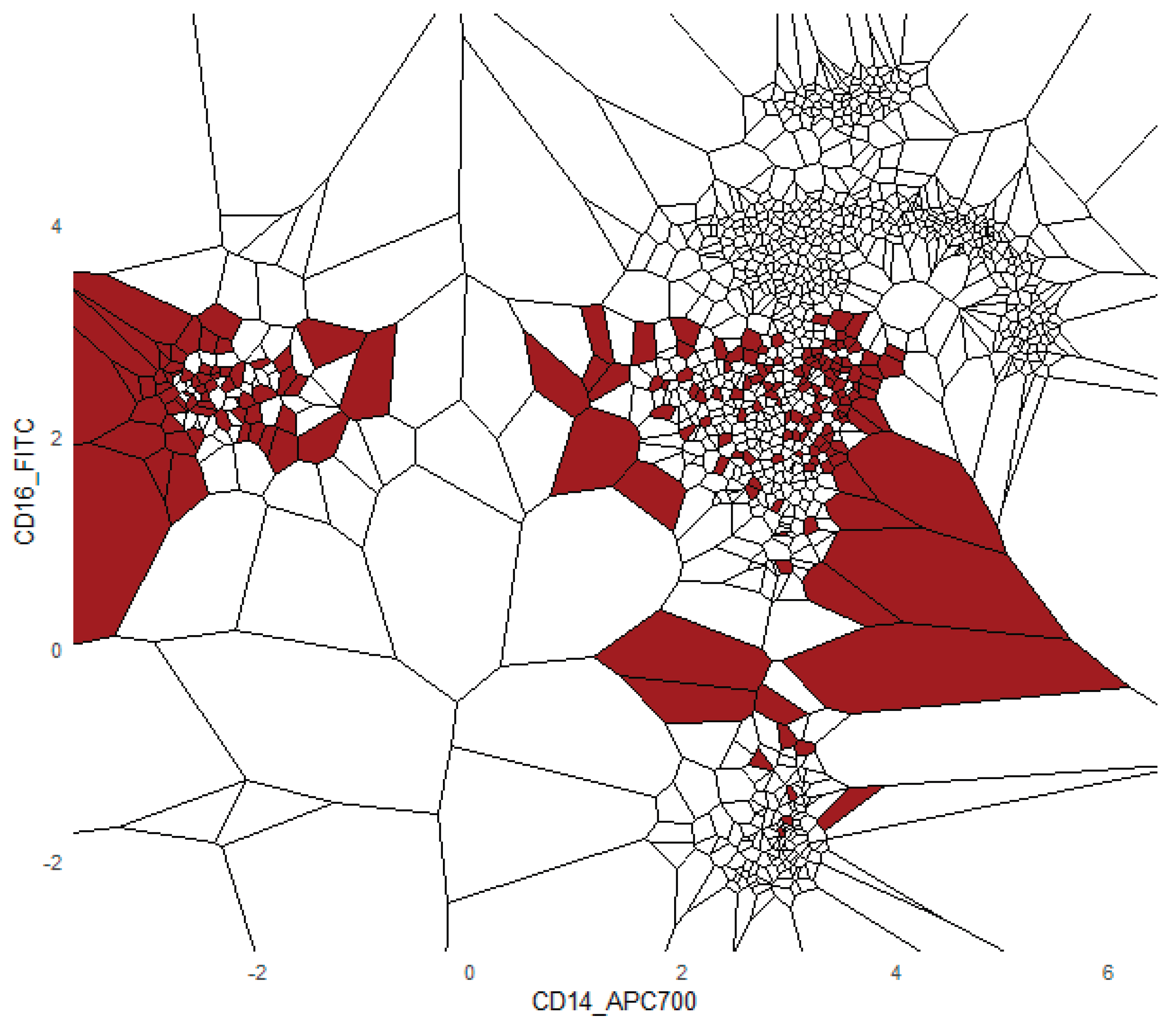
Figure 10.
The figure shows three customized 2D Voronoi per tessellation per class based on three population frequencies from the Dresden dataset. A depicts class bone marrow, and B depicts class blood. The low posterior values are in white. Dark red areas present high posterior values.
Figure 10.
The figure shows three customized 2D Voronoi per tessellation per class based on three population frequencies from the Dresden dataset. A depicts class bone marrow, and B depicts class blood. The low posterior values are in white. Dark red areas present high posterior values.
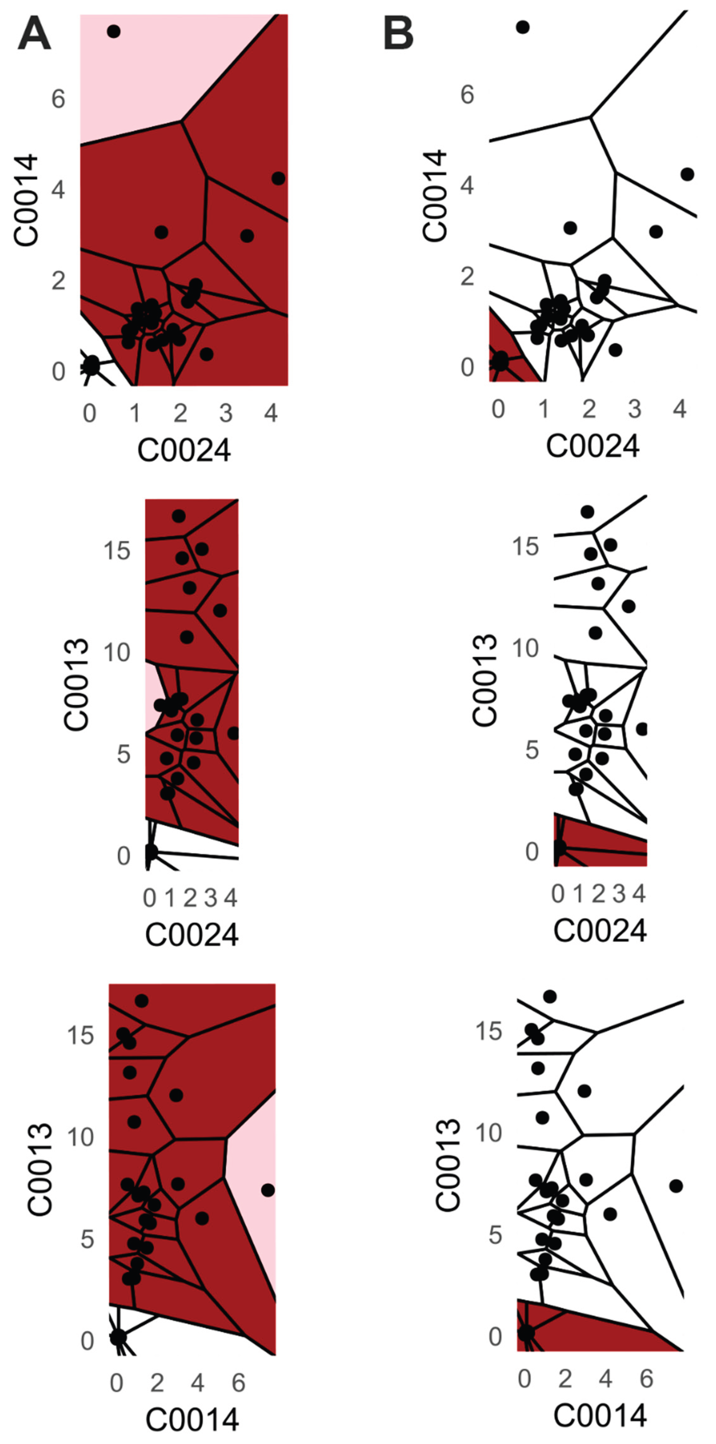

Table 1.
The table presents relevant meta information of the datasets used in the classification benchmark in the subsequent section. “N” states the number of cases, “DIM” the number of features, Class No. the number of classes, the number of cases per class, and the last four columns denote four different measures of dependency, namely Pearson’s correlation coefficient, Spearman’s Rank Correlation Coefficient, Kendall’s Tau, and Xi correlation coefficient. NA = not computable.
| N | DIM | Class No. | Cases per class | Pearson | Spearman | Kendall | XICOR | |
| Cell populations | 5121 | 14 | 13 | 1128, 312, 829, 525, 768, 122, 76, 135, 283, 630, 229, 31, 53 | 0-0.99 | 0-0.98 | 0-0.9 | 0-0.85 |
| Crabs (Sex) | 200 | 5 | 2 | 100, 100 | 0 | 0-0.07 | 0-0.03 | 0.01-0.24 |
| Crabs (SP) | 200 | 5 | 2 | 100, 100 | 0 | 0-0.07 | 0-0.03 | 0.01-0.24 |
| Dermatology | 358 | 34 | 6 | 111, 60, 71, 48, 48, 20 | 0-0.94 | 0-0.98 | 0-0.94 | 0-0.85 |
| Iris | 150 | 4 | 3 | 50, 50, 50 | 0.12-0.96 | 0.17-0.94 | 0.08-0.81 | 0.08-0.72 |
| MiceProtein | 1080 | 77 | 8 | 150, 150, 135, 135, 135, 135, 105, 135 | 0-1 | 0-1 | 0-1 | 0-0.99 |
| Penguins | 344 | 4 | 3 | 152, 68, 124 | 0 | 0-0.19 | 0-0.12 | 0-0.25 |
| Satellite | 6435 | 36 | 6 | 1533, 703, 1358, 626, 707, 1508 | 0-0.96 | 0-0.96 | 0.02-0.85 | 0.02-0.76 |
| Spam | 4601 | 57 | 2 | 2788, 1813 | 0-1 | 0-0.94 | 0-0.94 | 0-0.93 |
| Swiss | 200 | 6 | 2 | 100, 100 | 0.06-0.74 | 0.05-0.75 | 0.03-0.59 | 0.01-0.43 |
| Wine | 178 | 13 | 3 | 59, 71, 48 | 0-0.86 | 0.01-0.88 | 0.01-0.7 | 0-0.6 |
| WCBCD | 569 | 30 | 2 | 212, 357 | 0-1 | 0-1 | 0-0.99 | 0-0.97 |
| CoverType | 581012 | 55 | 7 | 211840, 283301, 35754, 2747, 9493, 17367, 20510 | 0-0.79 | 0-0.82 | NA | NA |
| LetterRecognition | 20000 | 16 | 26 | 796, 755, 805, 783, 773, 748, 766, 789, 747, 792, 787, 753, 758, 775, 736, 734, 752, 761, 803, 768, 764, 786, 783, 813, 739, 734 | 0-0.85 | 0-0.87 | NA | NA |
Table 2.
The table presents the final results of the classifiers performance evaluation. 14 datasets were evaluated (rows) and 8 classification algorithms were applied. The performance was evaluated with the Matthews Correlation Coefficient (MCC) and the mean (denoted as ) + AMAD (Adjust Mean Absolute Deviation) (denoted as ) is used to determine the overall performance.
| PDENB | GNB | NPNB | 7NN | PyGNB | klaRGNB | klaRNPNB | e1071GNB | |||||||||
| Cell populations | 0.98 | 0 | 0.97 | 0 | 0.98 | 0 | 0.16 | 0 | 0.97 | 0 | 0.97 | 0 | 0.98 | 0 | 0.97 | 0 |
| CoverType | 0.44 | 0 | 0.22 | 0 | 0.41 | 0 | 0.86 | 0 | 0.22 | 0 | 0.22 | 0 | 0.41 | 0 | 0.22 | 0 |
| Crabs (Sex) | 0.91 | 0.1 | 0.92 | 0.1 | 0.92 | 0.1 | 0.81 | 0.1 | 0.92 | 0.1 | 0.92 | 0.1 | 0.92 | 0 | 0.92 | 0.1 |
| Crabs (SP) | 0.99 | 0 | 0.99 | 0 | 0.97 | 0 | 0.88 | 0.1 | 0.99 | 0 | 0.99 | 0 | 0.97 | 0 | 0.99 | 0 |
| Dermatology | 0.95 | 0 | 0.82 | 0 | 0.9 | 0.1 | 0.81 | 0.1 | 0.85 | 0 | NA | NA | 0.9 | 0.1 | 0.82 | 0 |
| Iris | 0.95 | 0.1 | 0.94 | 0.1 | 0.94 | 0.1 | 0.95 | 0 | 0.94 | 0.1 | 0.94 | 0.1 | 0.94 | 0.1 | 0.94 | 0.1 |
| LetterRecognition | 0.72 | 0.1 | 0.66 | 0.1 | 0.72 | 0.1 | 0.18 | 0.1 | 0.66 | 0.1 | 0.66 | 0.1 | 0.72 | 0.1 | 0.66 | 0.1 |
| MiceProtein | 0.84 | 0 | 0.75 | 0 | 0.84 | 0 | NA | NA | NA | NA | NA | NA | NA | NA | 0.75 | 0 |
| Penguins | 0.98 | 0 | 0.98 | 0 | 0.97 | 0 | 0.97 | 0 | 0.98 | 0 | 0.98 | 0 | 0.97 | 0 | 0.98 | 0 |
| Spam | 0.68 | 0.1 | 0.52 | 0 | 0.38 | 0 | 0.58 | 0 | 0.68 | 0 | NA | NA | 0.37 | 0 | 0.52 | 0 |
| Satellite | 0.77 | 0 | 0.6 | 0 | 0.62 | 0 | 0.69 | 0 | 0.75 | 0 | 0.6 | 0 | 0.62 | 0 | 0.6 | 0 |
| Swiss | 0.98 | 0 | 0.99 | 0 | 0.99 | 0 | 0.98 | 0 | 0.99 | 0 | 0.99 | 0 | 0.99 | 0 | 0.99 | 0 |
| WCBCD | 0.89 | 0 | 0.89 | 0.1 | 0.87 | 0 | 0.93 | 0 | 0.89 | 0.1 | 0.89 | 0.1 | 0.88 | 0 | 0.89 | 0.1 |
| Wine | 0.97 | 0.1 | 0.96 | 0.1 | 0.96 | 0.1 | 0.95 | 0.1 | 0.96 | 0.1 | 0.96 | 0.1 | 0.96 | 0.1 | 0.96 | 0.1 |
Table 3.
The table presents the grades computed as the mean of the ranks. Ranks were obtained in the supplementary B based on the mean values of the study, where equal ranks are allowed and determined with a Permutation-Test.
Table 3.
The table presents the grades computed as the mean of the ranks. Ranks were obtained in the supplementary B based on the mean values of the study, where equal ranks are allowed and determined with a Permutation-Test.
| PDENB | PyGNB | NPNB | klaRNPNB | e1071GNB | GNB | kNN7 | klaRGNB | |
| Grade | 2.46 | 4 | 4.21 | 4.46 | 4.86 | 4.93 | 5.54 | 5.54 |
Disclaimer/Publisher’s Note: The statements, opinions and data contained in all publications are solely those of the individual author(s) and contributor(s) and not of MDPI and/or the editor(s). MDPI and/or the editor(s) disclaim responsibility for any injury to people or property resulting from any ideas, methods, instructions or products referred to in the content. |
© 2025 by the authors. Licensee MDPI, Basel, Switzerland. This article is an open access article distributed under the terms and conditions of the Creative Commons Attribution (CC BY) license (http://creativecommons.org/licenses/by/4.0/).
Copyright: This open access article is published under a Creative Commons CC BY 4.0 license, which permit the free download, distribution, and reuse, provided that the author and preprint are cited in any reuse.


