
Submitted:
05 June 2024
Posted:
06 June 2024
You are already at the latest version
Abstract
In metal additive manufacturing (AM), precise temperature field prediction is crucial for process monitoring, automation, control, and optimization. Traditional methods, primarily offline and data-driven, struggle with adapting to real-time changes and new process scenarios, which limits their applicability for effective AM process control. To address these challenges, this paper introduces the first physics-informed (PI) online learning framework specifically designed for temperature prediction in metal AM. Utilizing a physics-informed neural network (PINN), this framework integrates a neural network architecture with physics-informed inputs and loss functions.
Pretrained on a known process to establish a baseline, the PINN transitions to an online learning phase, dynamically updating its weights in response to new, unseen data. This adaptation allows the model to continuously refine its predictions in real-time. By integrating physics-informed components, the PINN leverages prior knowledge about the manufacturing processes, enabling rapid adjustments to process parameters, geometries, deposition patterns, and materials.
Empirical results confirm the robust performance of this PI online learning framework in accurately predicting temperature fields for unseen processes across various conditions. It notably surpasses traditional data-driven models, especially in critical areas like the Heat Affected Zone (HAZ) and melt pool. The PINN’s use of physical laws and prior knowledge not only provides a significant advantage over conventional models but also ensures more accurate predictions under diverse conditions. Furthermore, our analysis of key hyper-parameters—learning rate and batch size of the online learning phase—highlights their roles in optimizing the learning process and enhancing the framework’s overall effectiveness. This approach demonstrates significant potential to improve the online control and optimization of metal AM processes.
Keywords:
Physics-informed neural networks
; Metal additive manufacturing
; Online learning
; Real-time modeling
; Temperature field prediction
1. Introduction
Metal additive manufacturing (AM) introduces a paradigm shift in the field of manufacturing technologies, significantly enhancing adaptability across a range of sectors such as aerospace, biomedical engineering, and defense [1]. The capacity of this technology to construct detailed, tailor-made 3D configurations through sequential layer deposition not only enables the realization of mass customization but also facilitates the fabrication of components with reduced mass, optimized material consumption, and expedited prototype development [2].
Central to understanding and optimizing metal AM processes is the Parameter-Signature-Quality (PSQ) model, which explains the complex relations between the settings of the manufacturing process (Parameters), the observable effects during the process (Signatures), and the characteristics of the final product (Qualities). The PSP model serves as a critical framework, clarifying how variations in process parameters influence the physical and mechanical properties of the final product through changes in process signatures [3,4,5]. This relationship is key to ensuring that the manufacturing process yields parts that conform to predefined quality and performance standards, allowing for precise control over the variables to achieve the desired outcomes [6].
Temperature emerges as a vital signature in this framework, with its management and prediction being fundamental to the integrity and quality of AM parts [7,8]. In metal AM, the rapid heating and cooling cycles lead to significant temperature fluctuations within the substrate and deposited layers, affecting part quality and integrity through stress, distortion, and microstructural changes [9,10]. In addressing these challenges, real-time or near-real-time temperature prediction models are essential. They enable the dynamic adjustment of process parameters based on thermal feedback, thus enhancing thermal management and reducing defects for improved precision and quality of the final product [11].
Therefore, the capability to monitor and control temperature directly influences PSP dynamics, impacting thermal signatures and, consequently, the structural and material properties of manufactured components. By improving control over the AM process, these developments not only fulfill specific application requirements but also push the limits of manufacturing efficiency and product innovation in AM.
There has been extensive study on offline, data-driven approaches for thermal modeling in metal AM. Offline, or batch learning, is a method where models are trained on a complete dataset before deployment, without updating or learning from new data during operation. These studies have explored various methodologies for predicting temperature distributions and their effects on the final product’s quality, relying on historical data and computational simulations to inform their predictions. For instance, research by Pham et al. [12] developed a feed-forward neural network surrogate model to accurately predict temperature evolution and melting pool sizes in metal bulk samples made by the directed energy deposition (DED) process. In another work, Mozaffar et al. [13] developed a recurrent neural network (RNN)-based model to predict the thermal history of manufactured parts. Utilizing a considerable amount of data produced by the Finite Element Method (FEM), this model is adept at forecasting temperature fields both on the surface and within the interior of fabricated parts. Moreover, in [14], Le et al. used FEM data from five processes with different currents and voltages to train a neural network for temperature prediction at mesh points, using coordinates, travel speed, and current as inputs. The model, demonstrating over 99% accuracy, can predict temperature histories in new cases.
Adding to these conventional approaches, Physics-Informed Neural Networks (PINNs), as introduced by Raissi et al. [15], have emerged as a novel machine learning paradigm by integrating physical laws, typically described by partial differential equations (PDEs), directly into the neural network architecture. Notable implementations include the study by Zhu et al. [16], which utilized PINNs for temperature and melt pool dynamics in Laser Powder Bed Fusion (LPBF), and the research by Xie et al. [17], focusing on temperature prediction in DED. Additionally, Jiang et al. [18] demonstrated the effectiveness of PINNs in melt pool temperature predictions with limited training data. These instances underscore the potential of PINNs to improve predictive accuracy and computational efficiency in metal AM by employing physical principles, especially when faced with sparse data.
However, both traditional offline models and PINNs face shortcomings that limit their practicality within the evolving domain of metal AM. A shared challenge is their limited adaptability to real-time manufacturing variations, frequently leading to discrepancies between predicted outcomes and the dynamics of actual processes. These approaches struggle to generalize across the diverse AM processes characterized by different materials, geometries, and process parameters. Additionally, data-driven models require large training datasets, which are often not available in manufacturing. Meanwhile, PINNs, despite leveraging physical laws for prediction, typically focus on narrow segments of the AM process, which curtails their overall utility. Lastly, these models often require extensive computational resources and processing time for training, which can impede swift decision-making critical for optimizing AM processes in real time. For example, the processing time reported in [13] reached 40 hours, rendering it impractical for scenarios requiring real-time control.
Online learning, a branch of machine learning, updates model parameters dynamically with the arrival of new data, presenting a flexible alternative to conventional offline approaches. This method ensures the model stays relevant and accurate through real-time adaptation and is more efficient due to its reduced memory storage needs [19]. Unlike batch learning, which requires access to the entire dataset for training, online learning processes data incrementally, removing the need for substantial data storage. The benefits of online learning are evident across various fields. For example, Yang et al. [20] designed an Online Deep-Learning model for continuous monitoring of train traction motor temperatures, adjusting the model’s structure in response to new data. Wang et al. [21] proposed a combined method that leverages offline learning’s predictive capabilities with online learning’s adaptability for real-time control of deformable objects.
In the realm of metal AM, the application of online learning is emerging. Ouidadi et al. [22] applied online learning for real-time defect detection in Laser Metal Deposition (LMD), using transfer learning and adaptive models like K-means and self-organizing maps to enhance quality control by updating predictions with incoming data. Mu et al. [23] developed an online simulation model for Wire Arc Additive Manufacturing (WAAM) that employs neural network techniques to adapt predictions based on live data, showcasing an improvement over conventional models. Despite these advances, a significant gap exists in the specific application of online learning for thermal modeling within metal AM. To the authors’ best knowledge, this study is the first to explore physics-informed online learning for thermal modeling in metal AM, marking a pioneering step into this research area.
To this end, this paper introduces a framework that integrates a PINN with transfer learning and online learning to address the challenges of thermal modeling in metal AM. At its core, this methodology leverages real-time temperature field data alongside heat boundary conditions to accurately predict 2D temperature fields at future timestamps for processes previously unseen and for which no prior data is available before training. This novel approach is distinguished from prior methods by its dynamic adaptability to a wide array of AM scenarios, including variations in geometries, deposition patterns, and process parameters. This adaptability significantly improves the precision and utility of thermal field modeling in metal AM.
The key contributions of this study are as follows:
- Online Learning and Prediction: This study is potentially the first attempt to apply online learning for the real-time modeling and prediction of temperature fields in previously unseen AM processes. This pioneering effort represents an advancement towards adaptable manufacturing technologies.
- Physics-informed Integration: We have incorporated heat boundary conditions into our framework as physics-informed loss function, and heat input characteristics as physics-informed input within the neural network. This integration significantly increases the prediction accuracy and reliability.
- Framework Generality: Our methodology proves highly versatile, demonstrating effectiveness across a diverse range of AM conditions. It can accommodate changes in process parameters, materials, geometries, and deposition patterns, showcasing an essential step towards a universally adaptable AM framework.
- Improvement in Predictive Accuracy and Process Adaptability: By integrating real-time data with PINNs, this research enhances the predictive accuracy and adaptability of thermal models in metal AM. The framework’s dynamic adaptation to new data and varying conditions ensures precise temperature predictions, improving quality and consistency in AM processes. This advancement over existing methods enables more accurate and reliable thermal modeling, supporting the development of adaptable and efficient AM technologies.
The organization of the paper is as follows: Section 2 introduces the physics-informed online learning framework tailored for real-time temperature field prediction. Section 3 outlines the data generation and model implementation strategies. Section 4 discusses the results, emphasizing the framework’s capabilities and exploring potential limitations. Finally, Section 5 concludes the study, summarizing the contributions and suggesting future directions for enhancing the adaptability and precision of thermal modeling in metal AM.
2. Methodology
In this section, we delve into the development of the proposed physics-informed online learning framework aimed at the prediction of 2D temperature field in metal AM processes. The framework consists of two distinct phases. Initially, an offline learning phase where a PINN, incorporating a neural network with physics-informed modifications, is trained on a dataset from a previously conducted metal AM process. This initial phase enables the PINN to grasp the fundamental patterns and dynamics inherent in AM thermal processes, creating a robust foundation of knowledge for subsequent real-time data exposure.
In the online learning phase, this pre-trained PINN serves as the base model for dynamic adaptation to an unseen process, for which data is acquired in real time. The integration of Synaptic Intelligence (SI) [24] and an adaptive learning rate helps maintain and apply previously acquired knowledge as the PINN adapts to new data from different AM processes. This setup enables the PINN to dynamically update its weights through online gradient descent [25] in response to new information, demonstrating its flexibility and prompt response to temperature changes in the new process.
The PINN’s architecture consists of three core components: the neural network, physics-informed (PI) input, and a PI loss function. It employs a series of thermal images to predict the 2D temperature field at future time steps, which capture the 2D temperature fields of the currently deposited layer of the manufactured part, along with a PI input that includes heat input characteristics. More precisely, the model inputs a sequence of w thermal images spanning from timestamps to and the process’ heat input characteristics. It uses this data to forecast the thermal image (i.e., 2D temperature field) at the timestamp (. Here, w represents the window size of input data, capturing a specific range of thermal imaging, and i denotes the hyperparameter indicating the future timestamp targeted for prediction, focusing on the evolving thermal conditions of the currently deposited layer.
Figure 1 presents an overview of the proposed framework. We will further elaborate on this framework in the following sections: Section 2.1 delves into the components of the PINN; Section 2.2 discusses the pretraining phase, highlighting how the model is prepared using historical AM data. Finally, Section 2.3 covers the online learning phase, detailing the adaptation of the pre-trained PINN to new, real-time AM processes.
2.1. Proposed Physics-Informed Neural Network
The PINN used in our framework, detailed further in our previous paper [26], is a specialized neural network that incorporates Convolutional Long Short-Term Memory (ConvLSTM) layers and convolutional layers into the model’s architecture. It also includes an auxiliary input for process heat flux information, represented as a 2D matrix (i.e., PI input), and integrates a boundary condition (BC) loss term into the overall loss function (i.e., PI loss). Each component is essential for accurately predicting the thermal field by leveraging both data-driven insights and physics-informed constraints. In Figure 2, the proposed PINN, which comprises three key components: the neural network, PI loss, and PI input, is presented.
2.1.1. Neural Network Architecture
The architecture of the neural network is designed to capture the complexities of thermal field prediction within the domain of metal additive manufacturing. Central to this architecture are the Convolutional Long Short-Term Memory (ConvLSTM) layers, which can simultaneously process spatial and temporal information, making them an ideal choice for tasks addressed in this paper, where 2D thermal images serve as inputs, and the goal is to predict a 2D temperature distribution evolving over time. Complementing the ConvLSTM layers, the architecture also includes traditional convolutional layers. These layers specialize in extracting spatial features from each thermal image, identifying intricate patterns and temperature distributions essential for constructing an accurate predictive model. Together, these neural network components form a powerful and efficient architecture designed to tackle the challenges of predicting thermal fields in the dynamic environment of metal AM processes.
2.1.2. Physics-Informed Input
In our framework, the Physics-Informed (PI) input is incorporated to infuse the model with physics-based information regarding the heat input of the manufacturing process, thereby enabling the model to capture the intricate relationship between process parameters and the resultant temperature field. This addition ensures that the neural network can access a richer set of data that reflects the underlying physical processes, enhancing its ability to make better predictions. We choose the laser heat flux as the PI input. This parameter serves as a quantifiable measure of the energy intensity and distribution as the laser interacts with the material, which is vital for understanding the thermal dynamics involved in the process. The laser heat flux represents a critical factor that influences key thermal phenomena, including the melting and solidification processes and the creation of thermal gradients within the layer currently under fabrication.
The process of accurately estimating the laser heat flux is a cornerstone in enhancing our model’s predictive accuracy. Utilizing a Gaussian surface heat flux model [27] facilitates a nuanced representation of how the laser’s energy is dispersed across the material layer. This model incorporates critical factors such as laser power (P), the radius of the laser beam (), and the material’s absorptivity () to create a comprehensive picture of the energy input:
This equation calculates the heat flux (i.e., ) at each point on the material’s surface, based on the distance d from the laser center, effectively mapping out the spatial energy profile imposed by the laser. The precision in capturing this energy distribution is critical for simulating the thermal dynamics during the additive manufacturing process accurately. It allows our model to predict the resulting temperature fields with sufficient fidelity, considering how variations in laser settings or material properties could impact the thermal environment within the layer being printed. Figure 3 illustrates an instance of laser application on a surface, modeled using the Gaussian surface heat flux, along with its corresponding matrix.
2.1.3. Physics-Informed Loss
In our PINN, the PI loss function is essential to reflect the physical laws governing the system. The PI loss is designed to specifically enforce boundary conditions, which are critical for accurately modeling thermal processes in metal additive manufacturing.
Boundary conditions dictate how surfaces of a part interact with their environment, influencing heat transfer mechanisms such as conduction, convection, and radiation, crucial for predicting temperature fields during manufacturing. The PI loss minimizes the residual of the physical equations at these boundaries, improving the network’s adherence to physical constraints and ensuring predictions are both statistically accurate and physically plausible.
By penalizing deviations from these physical laws, our model’s reliability is bolstered. For the problem of predicting the 2D temperature field of the currently deposited layer, the specific boundary condition for the top surface is mathematically expressed as follows:
In this equation, T denotes the matrix of the 2D temperature fields, representing the temperature distribution during the manufacturing process captured by thermal images. This equation encompasses several heat transfer mechanisms: The term calculates the conductive heat flux through the surface, with denoting the normal direction outward from the surface. is the convective heat transfer coefficient, modeling heat loss due to air or fluid motion over the surface. Radiative heat loss is given by , where is the Stefan-Boltzmann constant and is the emissivity, indicating energy lost as radiation based on the fourth power of the temperature difference between the surface and ambient air. represents the heat input from the laser, crucial for the melting and fusing of material layers.
Given the boundary condition, the residual for the boundary condition can be defined as:
The PI loss, , is computed as the mean squared error of the residuals across N thermal images:
The total loss function for the PINN, which includes both the data-based loss () and the physics-informed loss (), is weighted to balance the contribution from each component. The weights for each loss term, for and for , are established during the training process. This involves observing and adjusting the impact of each loss term to ensure they contribute equally to the overall loss. The combined loss function is expressed as follows:
Here, and denote the weights assigned to the PI loss and data loss, respectively. These weights are proportionally set to balance the scale between two terms in the loss function, contributing to improved training robustness of the model.
2.2. Offline Learning Stage
In the offline learning stage, our framework trains a PINN on data from a completed metal AM process. This training integrates physics-based inputs and loss functions tailored to the specific material properties and heat input characteristics of the process, equipping the model with an understanding of the underlying thermal dynamics. This comprehensive preparation sets a solid foundation for the model’s subsequent application in the online learning stage.
The PI loss function in our framework incorporates material properties—thermal conductivity (k) and convection heat transfer coefficient (), determined by the materials used in the process. These properties are crucial for enforcing realistic boundary behaviors for accurate thermal modeling. Additionally, heat input parameters such as laser power (P), beam radius (), and material absorptivity (), are integrated into a physics-informed input that characterizes the laser heat flux.
As the model transitions to the online learning phase, it requires careful management of model updates to ensure that new data does not drastically alter the neural network’s established weight configurations. It is essential to maintain the network’s fundamental knowledge from the offline learning phase, enabling it to adjust to new data while preserving its accuracy and ability to predict temperature fields as taught by historical data. Synaptic Intelligence addresses this by evaluating the significance of each weight relative to the tasks mastered previously. This evaluation is captured mathematically by omega values (), which highlight weights that are key to the model’s prior tasks and should therefore be conservatively adjusted with incoming data.
Here, is the omega value for weight i, is the gradient of the loss with respect to weight i at time t, is the change in weight i at time t, and is the total change in weight i over the training period. To streamline computation and avoid potential issues like division by zero, an approximation is used:
This approach posits that the importance of weight is indicated by the sum of its gradients’ magnitudes over time, implying that weights with consistently significant gradients are more important for the model’s function than otherwise.
Incorporating these omega values into the online learning phase allows the model to adjust weight importance flexibly, integrating new data while maintaining the core insights gained previously. The careful balance between incorporating new information and preserving valuable existing knowledge improves the model’s adaptability and performance across varied additive manufacturing scenarios.
2.3. Online Learning Stage
In the online learning phase, the primary objective is to predict the temperature field for a new, previously unseen metal AM process that may exhibit characteristics different from the process used during the offline learning stage. This phase is crucial for allowing the model to transition smoothly from utilizing foundational knowledge to integrating new insights, thus maintaining accuracy and adaptability during the dynamic conditions of AM processes. A critical aspect of this phase involves updating the PI input and PI loss function to incorporate new process characteristics as they are encountered. For instance, modifications in laser power, material properties, or beam radius require adjustments to the PI input that captures the laser heat flux and the PI loss terms that enforce adherence to new boundary conditions and material behaviors. By dynamically adapting these PI components to reflect new process characteristics, the model effectively incorporates updated knowledge, enhancing its accuracy and adaptability across different AM setups.
In this phase, the PINN, previously trained during the offline learning stage, serves as the initial model. Its weights are updated in real time as new data from the ongoing process is received. The PINN employs online gradient descent (OGD) to dynamically adapt to new data. This method allows for immediate adjustments to the model’s parameters, enhancing its ability to refine predictions continuously as new information becomes available. The mathematical expression for updating the weights through OGD is shown below:
where and represent the weights before and after processing the new data point, respectively. The learning rate, , determines the step size for the update, and is the gradient of the loss function relative to the weights for the current data point and its target value .
The loss function used during this phase includes components for data loss (), PI loss (), and Synaptic Intelligence (SI) loss () :
where , is specifically formulated as follows:
Here, , , and are the weights that are determined during the training process to maintain a balanced scale among the various terms in the loss function. quantifies the importance of each weight i in the neural network, reflecting its role in prior tasks learned by the model. The term measures the change in weight i due to new data, and squaring this change aims to minimize large shifts in critical weights, thus preserving essential knowledge and mitigating catastrophic forgetting. This strategic formulation ensures that the model not only adapts to new data but also retains accuracy and stability in predictions by balancing novel learning with the preservation of previously acquired knowledge.
Additionally, we adjust the learning rate dynamically, starting with a lower value to prevent drastic parameter shifts when limited data is available. This conservative approach maintains model stability. As more data is integrated and the model adapts, we increase the learning rate to accelerate learning and enhance adaptability, ensuring the model remains responsive to new information while preserving its accuracy.
3. Data Generation and Model Implementation
In this section, we outline the dataset generation using simulation, emphasizing the distinct characteristics of these simulations. We utilized finite element simulations with ANSYS software, specifically the Workbench AM DED 2022 R2 module, to create the training and testing datasets for our online learning framework. We conducted a total of five simulations, varying materials, geometries, deposition patterns, and process parameters to evaluate the framework’s generalizability under diverse conditions.
These simulations standardized the pass width and layer thickness at a consistent 1 mm. Materials such as 17–4PH stainless steel and Inconel 625 were chosen for their prevalent use and unique properties pertinent to our study. Geometrically, cylinders and cubes were explored for their common industrial applications, and three distinct deposition patterns were investigated to further assess the framework’s flexibility.
For process parameters, we defined two distinct scenarios: one with a deposition speed of 10 mm/s and a higher laser power, and another at 6 mm/s with a lower laser power. Our thermal analysis incorporated factors such as thermal conductivity, convection, and radiation, maintaining substrate and ambient temperatures at a constant 23°C. Activation temperatures were set at 2000°C for the lower laser power and 2400°C for the higher laser power, noting that the simulation abstracts from directly modeling the laser’s heat flux. An overview of different simulated processes A-D is illustrated in Table 1.
Each simulation produced datasets capturing transient temperature values at each timestamp, from which approximately 16,000 input-output pairs per simulation were extracted for training and validation. These pairs consisted of sequences of the 2D temperature field for the currently deposited layer as inputs, with the outputs representing the 2D temperature field of the same layer for the subsequent timestamp.
The model is implemented in TensorFlow. We constructed a neural network with six ConvLSTM layers and four convolutional layers, each utilizing 20 filters. This network was pre-trained using data from the simulated processes, with a learning rate set to . The pretraining phase employed three previous timestamps () to predict the temperature field five seconds ahead (). Upon completing pretraining, both the model’s parameters and the omegas for each parameter were saved. These omegas indicate the importance of the weights in retaining learned knowledge, vital for the subsequent online learning phase.
In the online learning stage, the architecture remains unchanged, and the pre-trained model, equipped with the saved weights, is introduced to streaming data from a new process simulation.
Based on the insights from Section 4, the learning rate is dynamically adjusted throughout the phase, starting at and incrementally increasing to to better accommodate learning from the dynamic, real-time data. While setting to 1, the regularization parameter is set to to balance the scales of the data loss () and the Synaptic Intelligence loss (), ensuring harmony between adapting to new information and preserving essential insights from previous learning. Similarly, is set to to align the Physics-Informed loss () with the other terms in the loss function, maintaining consistency across the model’s evaluation criteria. This calibration supports the neural network to be effectively trained on the fly with the new process data, ensuring the model’s continuous adaptation and robustness in predicting temperature fields across varied additive manufacturing scenarios.
4. Results and Discussion
To evaluate the real-time adaptability of our online learning framework to new data, we carried out a sequence of experiments. We designated Process A (Table 1) as the baseline dataset for the offline learning phase, creating a foundational knowledge base for the model to understand the standard thermal patterns of metal AM processes. We then transitioned to the online learning phase, progressively introducing datasets from Processes B, C, and D (Table 1). Each dataset represented a unique scenario and varied incrementally from the parameters of Process A.
The experimental processes were strategically designed to evaluate the performance of the online learning framework under various scenarios: Process B mirrored Process A, differing only in specific operational parameters to test the model’s sensitivity to such changes under controlled conditions. Process C presented a greater challenge by varying not only the process parameters but also the deposition patterns, assessing the model’s adaptability to both thermal and process changes. Process D, introducing a change in geometry and material, represented the most significant departure from the initial setup, testing the model’s ability to adapt predictions to new structural contexts.
To evaluate the model’s performance, we used Mean Absolute Error (MAE) and Mean Absolute Percentage Error (MAPE). The mathematical representations for the metrics are as follows:
In these equations, and denote the actual and predicted temperature values for each element in the 2D temperature field, respectively, with n and m representing the number of rows and columns in the temperature matrix. The individual errors calculated by these metrics provide insights into the precision at each data point, while the overall error for the validation dataset, obtained by averaging these individual errors, offers an evaluation across the entire dataset.
4.1. Performance of Physics-Informed Online Learning
The performance evaluation of the Physics-Informed (PI) model during the online learning phase involves a structured training procedure. The dataset from each process—B, C, and D—is split such that the first 80% is used incrementally as the training set, allowing the model to continuously update and refine its predictions. The remaining 20% of the data serves as the validation set, used to assess the model’s predictive accuracy and to validate its generalization capability on unseen data.
The model’s ability to process new batches of data swiftly is a significant advantage, particularly in real-time applications. On average, updating the model with a new batch of data takes just 0.21 seconds on Compute Canada’s infrastructure using a single NVIDIA Tesla T4 GPU. This demonstrates the framework’s efficiency and practical utility in scenarios where rapid data processing and immediate decision-making are crucial.
In Figure 4, the MAPE and MAE are illustrated, providing clear visual indicators of the model’s performance across various stages of the learning process. These metrics are plotted against the percentage of process data that has been incrementally introduced to the model, which is represented on the x-axis. The y-axis, meanwhile, displays the values of MAPE or MAE, indicating the model’s error rate at each stage of data integration.
For Process B, the initial spike in MAPE suggests an adjustment period as the model adapts to changes in process parameters. As more data is processed, a steady decrease in error is observed, highlighting the framework’s capacity to learn and refine its predictions based on closely related baseline conditions. In contrast, Process C, with its introduction of new deposition patterns in addition to varied process parameters, starts with a higher MAPE. This underscores the complexity introduced by the new material properties and deposition strategies. However, the subsequent decline in MAPE indicates effective model adaptation to these complexities, showcasing its ability to manage multi-faceted changes in AM processes.
Process D shows an initially high MAPE, reflecting the challenge of accommodating a new material and geometric configuration, but this quickly improves as the model assimilates more data and fine-tunes its predictions to the altered geometry. Despite Process B’s closer resemblance to Process A, the modeling for Process D results in lower errors than for Process B. This could be attributed to the circular deposition patterns in Processes A and B, which may complicate thermal management due to surface curvature affecting heat conduction and convection, thereby posing greater modeling challenges than the uniform cubic geometry of Process D.
4.2. Comparison of Proposed Framework with Machine Learning Framework
In this section, we conduct a comparative analysis between the physics-informed (PI) online learning framework and a data-driven approach. As outlined in Section 2.1, the PINN model that is used in the PI framework incorporates three main components: the neural network architecture, physics-informed (PI) inputs, and physics-informed (PI) loss function. In contrast, the data-driven model used for comparison utilizes the same neural architecture but excludes the PI components, focusing solely on data-centric learning methods.
To ensure a comprehensive evaluation, we assess the performance of both the PI and data-driven frameworks across two critical areas: the entire temperature field of the layer being deposited, and specifically within the Heat Affected Zone (HAZ) and melt pool area. The HAZ is a crucial region in metal AM processes, characterized by the surrounding material of the weld or melt pool that experiences thermal cycling without melting. This zone is drastically influential in microstructural changes due to thermal exposure, which can significantly impact the mechanical properties and integrity of the final product [28]. Accurate identification and management of the HAZ and melt pool are essential for ensuring the quality of manufactured components.
The literature indicates that identification of the HAZ in AM processes typically involves sophisticated methods such as thermal imaging, metallurgical analysis, and computational modeling. In our study, the HAZ is defined as the region where the temperature exceeds a specific threshold that modifies the microstructure. For materials like 17–4PH stainless steel and Inconel 625, the HAZ temperature thresholds are set at 1050°C [29] and 960°C [30], respectively, reflecting their unique thermal characteristics. These established thresholds facilitate the analysis of both the HAZ and melt pool, crucial for the comparative evaluation of the frameworks in our study.
Figure 5 presents the MAPE of both PI and data-driven frameworks as they predict temperature fields across the entire deposited layer (upper row), the melt pool, and the surrounding HAZ (lower row). In Process B, the PI framework consistently outperforms the data-driven model, exhibiting lower errors when predicting the temperature field for future timestamps as it continuously integrates new data. However, for Processes C and D, despite the PI model initially showing lower error rates—thanks to the incorporation of physics-based knowledge during training—the data-driven model achieves slightly lower MAPE in the latter half of the process. This shift can be attributed to the additional requirements imposed by the physics-informed constraints in the PI model, which slightly decelerates error reduction.
Regarding the specific areas of the HAZ and melt pool, the PI framework maintains superior performance throughout the online learning process, consistently presenting lower error rates compared to its data-driven counterpart. Notably, the disparity between the PI and data-driven models is more noticeable at the beginning of the online learning phase when less data is available. This underscores the significant advantage of incorporating prior physical knowledge into the neural network, which enhances initial model guidance and prediction accuracy at the early stages. It is important to note that the error rates for both models are generally higher in the HAZ and melt pool areas. This increased error is due to the more complex thermal behavior in these zones, influenced by phenomena such as steep thermal gradients, rapid solidification rates, and varied material properties at high temperatures. These factors complicate the thermal dynamics, making accurate predictions more challenging [16].
The comparative analysis between the PI and the data-driven frameworks is further elucidated by examining their respective outputs against the ground truth provided by simulations. Figure 6 illustrate the predicted temperature fields for both the PINN and data-driven models alongside the simulated "true" temperature distributions for process C.
In the provided examples, both the PI and data-driven frameworks align variably with the simulation results, with most predicted temperatures differing by less than 20°C from the simulated temperature. Near the melt pool, discrepancies increase, though the PI model generally approximates simulated values more closely, especially around critical areas like the HAZ and melt pool itself. This precision is indicative of the PINN’s ability to incorporate physical laws into its predictions of complex phenomena in metal AM processes.
The figure also displays the absolute difference panels, which quantify the discrepancies between the predictions and the simulations. These discrepancies highlight areas where the models struggle to capture the exact thermal behaviors, potentially due to the intricate dynamics within the melt pool and HAZ that are challenging to model precisely with data-driven approaches alone.
The “HAZ + Melt Pool MAPE” images further provide a focused view of the error distribution within the HAZ, emphasizing the regions where the predictions deviate most significantly from the observed data. This detailed error analysis is critical for refining the models and for understanding the specific conditions under which each model may require further tuning or additional data to enhance accuracy.
In these comparisons, the PI framework consistently outperforms the data-driven framework, particularly in critical areas such as the HAZ and melt pool, where precise temperature knowledge is crucial for ensuring the quality and integrity of the manufactured parts. This superiority of the PI framework is especially significant when considering that the provided examples are outputs at a stage where only 80% of the data from the new process has been integrated into the models, as indicated in Figure 5. It is noteworthy that the PI framework’s performance advantage becomes even more pronounced when less data is available, underscoring its robust capability to effectively utilize physical laws to predict complex phenomena with limited input data. This makes the PI model particularly valuable in the early stages of new process integration, where data scarcity can often hinder accurate modeling.
4.3. Effect of Varying Learning Rates
This section evaluates the impact of different learning rate strategies on the performance of the PI framework during its online learning stage. As the model transitions from pretraining on a previous process’s data to incremental data from a new process, selecting an optimal learning rate strategy becomes critical for managing adaptability and accuracy.
We explore three main learning rate strategies: constant, linear increasing, and decreasing. A constant learning rate strategy provides a stable update mechanism throughout the learning process, suitable for environments where data properties do not vary significantly. A linear increasing learning rate strategy allows the model to start with cautious adjustments and progressively increase its responsiveness as it adapts to the new data. Conversely, a linear decreasing learning rate strategy enables the model to initially make broad updates and gradually refine these adjustments to focus on detailed patterns.
Figure 7 illustrates the MAPE for these strategies, showcasing how each one impacts model accuracy over the training period.
The constant learning rate was set at , a value carried over from the offline learning stage to provide a baseline of stability. In the increasing learning rate strategy, the learning rate began at a much lower value, , intentionally chosen to demonstrate the effect of gradually adapting the learning rate on the model’s performance. This strategy proved particularly beneficial as it allowed the model to adjust more significantly as its confidence in the new data increased, leading to a consistent reduction in error rates throughout the training process. By gradually increasing the learning rate, this approach helps prevent stagnation, ensuring that the model remains dynamic and responsive as it encounters new and increasingly complex data. This calibration of learning rate adjustments fosters a more gradual adaptation to new data, enabling the model to evolve its learning strategy in sync with the unfolding complexities of the process. On the other hand, the decreasing learning rate started at , aiming to quickly assimilate broad patterns before reducing the rate to . However, this approach occasionally resulted in higher error rates in training, indicating that a high initial rate might compromise the model’s ability to adapt to new complexities as they arise.
The analysis indicates that the choice of learning rate strategy and its initial setting plays an important role in the model’s ability to adapt to new data. Among the strategies examined, the increasing learning rate strategy not only facilitated better initial learning with minimal risk of error escalation but also allowed for enhanced adaptability and precision as the complexity of the data increased. This strategy’s success underscores the importance of a dynamic learning rate adjustment in environments where data characteristics are expected to evolve substantially, such as in metal AM.
4.4. Effect of Varying Batch Sizes
In this section, we explore the impact of varying batch sizes of new online data on the performance of PI online learning framework, specifically focusing on batch sizes of 2, 4, 8, 16, and 32. The batch size is a critical hyperparameter in machine learning that determines the number of training examples used in one iteration to calculate the gradient during the model training process. This parameter significantly influences both the computational efficiency and the convergence behavior of the training algorithm.
The Figure 8 illustrates the MAPE for different batch sizes across Processes B, C, and D. This visualization helps assess how the batch size impacts model accuracy and learning dynamics during the online training phase. The results reveal that as the batch size increases, there is a noticeable stabilization in error reduction throughout the online learning process. Larger batch sizes tend to smooth out the learning updates due to the averaging of gradients across more data points. This aggregation diminishes the influence of outliers and reduces the variability of weight updates, leading to a more consistent and gradual decrease in error rates.
Moreover, larger batch sizes offer computational advantages, particularly for real-time applications. Processing larger batches can utilize computational resources more efficiently, potentially speeding up the training process since fewer updates are required per epoch. However, this comes with the caveat that the model must wait for the entire batch of data to be collected and processed before proceeding with an update. This requirement can introduce delays in scenarios where data is being gathered incrementally, such as in real-time monitoring or streaming applications. Hence, there is a trade-off between computational speed and update latency that needs to be carefully managed to optimize real-time performance.
In conclusion, the choice of the batch size is a decision that balances several factors, including error stability, computational efficiency, and responsiveness to new data. Larger batches may be preferable for scenarios where computational speed is crucial and data is abundant, but they require careful consideration of the delay in model updates.
5. Conclusion
In this paper, we introduce the first physics-informed (PI) online learning framework specifically designed for temperature field prediction in metal additive manufacturing (AM), utilizing a physics-informed neural network (PINN). This innovative framework integrates a PINN, which includes three main components—neural network architecture, physics-informed inputs, and physics-informed loss functions. Initially, the PINN is pretrained on a known process during the offline learning stage to establish a foundational model. It then transitions to the online learning stage where it continuously adapts to new, unseen process data by dynamically updating its weights.
The integration of physics-informed components enables the model to effectively utilize prior knowledge about the processes involved, significantly enhancing its performance right from the outset of the online learning phase. This is particularly beneficial for rapidly adapting to new conditions and variations in process parameters, geometries, deposition patterns, and materials without extensive retraining.
Our results demonstrate the robust performance of the PI online learning framework in predicting temperature fields for unseen processes, effectively handling various manufacturing conditions. Particularly notable is its superior performance over data-driven counterparts in predicting temperatures in critical areas such as the Heat Affected Zone (HAZ) and melt pool. These regions are vital for the overall quality and structural integrity of the manufactured parts, highlighting the importance of precise temperature predictions in these areas. The PINN’s integration of physical laws and prior knowledge provides a distinct advantage, enabling more accurate predictions under diverse conditions. Additionally, our analysis of key operational parameters—including learning rate and batch size of the online learning process—reveals their roles in optimizing the learning process, further enhancing the framework’s effectiveness.
In conclusion, this study represents a pioneering effort in applying physics-informed online learning to metal AM, offering significant improvements in predictive accuracy and operational efficiency. Looking ahead, experimental data from actual metal AM processes can be integrated to enhance the physics-informed machine learning framework. The incorporation of real-world data is expected to improve the accuracy of the model’s predictions by capturing the complex and nuanced behaviors of AM environments.
Acknowledgments
This work was supported by the Natural Sciences and Engineering Research Council (NSERC) of Canada, under Grant No. RGPIN-2019-06601. Additionally, we acknowledge the use of generative AI tools, specifically ChatGPT, for light editing assistance, including spelling and grammar corrections.
References
- Ford, S.; Despeisse, M. Additive manufacturing and sustainability: an exploratory study of the advantages and challenges. Journal of cleaner Production 2016, 137, 1573–1587. [Google Scholar] [CrossRef]
- Cooke, S.; Ahmadi, K.; Willerth, S.; Herring, R. Metal additive manufacturing: Technology, metallurgy and modelling. Journal of Manufacturing Processes 2020, 57, 978–1003. [Google Scholar] [CrossRef]
- Shrestha, R.; Shamsaei, N.; Seifi, M.; Phan, N. An investigation into specimen property to part performance relationships for laser beam powder bed fusion additive manufacturing. Additive Manufacturing 2019, 29, 100807. [Google Scholar] [CrossRef]
- Sames, W.J.; List, F.; Pannala, S.; Dehoff, R.R.; Babu, S.S. The metallurgy and processing science of metal additive manufacturing. International materials reviews 2016, 61, 315–360. [Google Scholar] [CrossRef]
- Mani, M.; Lane, B.M.; Donmez, M.A.; Feng, S.C.; Moylan, S.P. A review on measurement science needs for real-time control of additive manufacturing metal powder bed fusion processes. International Journal of Production Research 2017, 55, 1400–1418. [Google Scholar] [CrossRef]
- Dehaghani, M.R.; Sahraeidolatkhaneh, A.; Nilsen, M.; Sikström, F.; Sajadi, P.; Tang, Y.; Wang, G.G. System identification and closed-loop control of laser hot-wire directed energy deposition using the parameter-signature-quality modeling scheme. Journal of Manufacturing Processes 2024, 112, 1–13. [Google Scholar] [CrossRef]
- Thompson, S.M.; Bian, L.; Shamsaei, N.; Yadollahi, A. An overview of Direct Laser Deposition for additive manufacturing; Part I: Transport phenomena, modeling and diagnostics. Additive Manufacturing 2015, 8, 36–62. [Google Scholar] [CrossRef]
- Masoomi, M.; Pegues, J.W.; Thompson, S.M.; Shamsaei, N. A numerical and experimental investigation of convective heat transfer during laser-powder bed fusion. Additive Manufacturing 2018, 22, 729–745. [Google Scholar] [CrossRef]
- Bontha, S.; Klingbeil, N.W.; Kobryn, P.A.; Fraser, H.L. Thermal process maps for predicting solidification microstructure in laser fabrication of thin-wall structures. Journal of materials processing technology 2006, 178, 135–142. [Google Scholar] [CrossRef]
- Barua, S.; Liou, F.; Newkirk, J.; Sparks, T. Vision-based defect detection in laser metal deposition process. Rapid Prototyping Journal 2014, 20, 77–85. [Google Scholar] [CrossRef]
- Yan, Z.; Liu, W.; Tang, Z.; Liu, X.; Zhang, N.; Li, M.; Zhang, H. Review on thermal analysis in laser-based additive manufacturing. Optics & Laser Technology 2018, 106, 427–441. [Google Scholar]
- Pham, T.Q.D.; Hoang, T.V.; Van Tran, X.; Pham, Q.T.; Fetni, S.; Duchêne, L.; Tran, H.S.; Habraken, A.M. Fast and accurate prediction of temperature evolutions in additive manufacturing process using deep learning. Journal of Intelligent Manufacturing 2023, 34, 1701–1719. [Google Scholar] [CrossRef]
- Mozaffar, M.; Paul, A.; Al-Bahrani, R.; Wolff, S.; Choudhary, A.; Agrawal, A.; Ehmann, K.; Cao, J. Data-driven prediction of the high-dimensional thermal history in directed energy deposition processes via recurrent neural networks. Manufacturing letters 2018, 18, 35–39. [Google Scholar] [CrossRef]
- Le, V.T.; Bui, M.C.; Pham, T.Q.D.; Tran, H.S.; Van Tran, X. Efficient prediction of thermal history in wire and arc additive manufacturing combining machine learning and numerical simulation. The International Journal of Advanced Manufacturing Technology 2023, 126, 4651–4663. [Google Scholar] [CrossRef]
- Raissi, M.; Perdikaris, P.; Karniadakis, G.E. Physics-informed neural networks: A deep learning framework for solving forward and inverse problems involving nonlinear partial differential equations. Journal of Computational physics 2019, 378, 686–707. [Google Scholar] [CrossRef]
- Zhu, Q.; Liu, Z.; Yan, J. Machine learning for metal additive manufacturing: predicting temperature and melt pool fluid dynamics using physics-informed neural networks. Computational Mechanics 2021, 67, 619–635. [Google Scholar] [CrossRef]
- Xie, J.; Chai, Z.; Xu, L.; Ren, X.; Liu, S.; Chen, X. 3D temperature field prediction in direct energy deposition of metals using physics informed neural network. The International Journal of Advanced Manufacturing Technology 2022, 119, 3449–3468. [Google Scholar] [CrossRef]
- Jiang, F.; Xia, M.; Hu, Y. Physics-Informed Machine Learning for Accurate Prediction of Temperature and Melt Pool Dimension in Metal Additive Manufacturing. 3D Printing and Additive Manufacturing 2023. [Google Scholar] [CrossRef]
- Hoi, S.C.; Sahoo, D.; Lu, J.; Zhao, P. Online learning: A comprehensive survey. Neurocomputing 2021, 459, 249–289. [Google Scholar] [CrossRef]
- Yang, Z.; Dong, H.; Man, J.; Jia, L.; Qin, Y.; Bi, J. Online Deep Learning for High-Speed Train Traction Motor Temperature Prediction. IEEE Transactions on Transportation Electrification 2023. [Google Scholar] [CrossRef]
- Wang, C.; Zhang, Y.; Zhang, X.; Wu, Z.; Zhu, X.; Jin, S.; Tang, T.; Tomizuka, M. Offline-online learning of deformation model for cable manipulation with graph neural networks. IEEE Robotics and Automation Letters 2022, 7, 5544–5551. [Google Scholar] [CrossRef]
- Ouidadi, H.; Guo, S.; Zamiela, C.; Bian, L. Real-time defect detection using online learning for laser metal deposition. Journal of Manufacturing Processes 2023, 99, 898–910. [Google Scholar] [CrossRef]
- Mu, H.; He, F.; Yuan, L.; Hatamian, H.; Commins, P.; Pan, Z. Online distortion simulation using generative machine learning models: A step toward digital twin of metallic additive manufacturing. Journal of Industrial Information Integration 2024, 38, 100563. [Google Scholar] [CrossRef]
- Zenke, F.; Poole, B.; Ganguli, S. Continual learning through synaptic intelligence. International conference on machine learning. PMLR, 2017, pp. 3987–3995.
- Zinkevich, M. Online convex programming and generalized infinitesimal gradient ascent. Proceedings of the 20th international conference on machine learning (icml-03), 2003, pp. 928–936.
- Sajadi, P.; Dehaghani, M.R.; Tang, Y.; Wang, G.G. Real-Time 2D Temperature Field Prediction in Metal Additive Manufacturing Using Physics-Informed Neural Networks. arXiv preprint arXiv:2401.02403, arXiv:2401.02403 2024.
- Al Hamahmy, M.I.; Deiab, I. Review and analysis of heat source models for additive manufacturing. The International Journal of Advanced Manufacturing Technology 2020, 106, 1223–1238. [Google Scholar] [CrossRef]
- Saboori, A.; Aversa, A.; Marchese, G.; Biamino, S.; Lombardi, M.; Fino, P. Microstructure and mechanical properties of AISI 316L produced by directed energy deposition-based additive manufacturing: A review. Applied sciences 2020, 10, 3310. [Google Scholar] [CrossRef]
- Cheruvathur, S.; Lass, E.A.; Campbell, C.E. Additive manufacturing of 17-4 PH stainless steel: post-processing heat treatment to achieve uniform reproducible microstructure. Jom 2016, 68, 930–942. [Google Scholar] [CrossRef]
- Wang, S.; Gu, H.; Wang, W.; Li, C.; Ren, L.; Wang, Z.; Zhai, Y.; Ma, P. The influence of heat input on the microstructure and properties of wire-arc-additive-manufactured Al-Cu-Sn alloy deposits. Metals 2020, 10, 79. [Google Scholar] [CrossRef]
Figure 1.
Schematic of the two-stage framework for online 2D temperature prediction in metal AM. Both stages leverage physics-informed components based on process parameters and material to guide the PINN: initially through training on previous AM thermal patterns, and subsequently through updates with real-time thermal images.
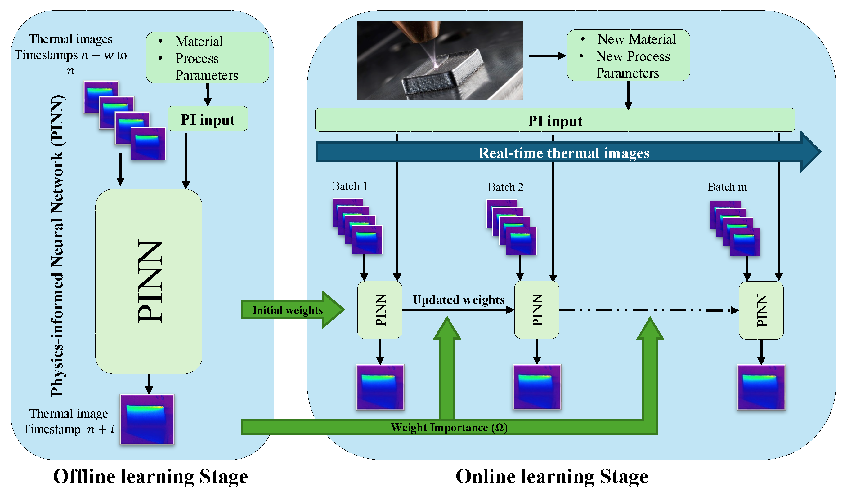
Figure 2.
PINN with its components: the neural network, PI-input, and PI-loss.
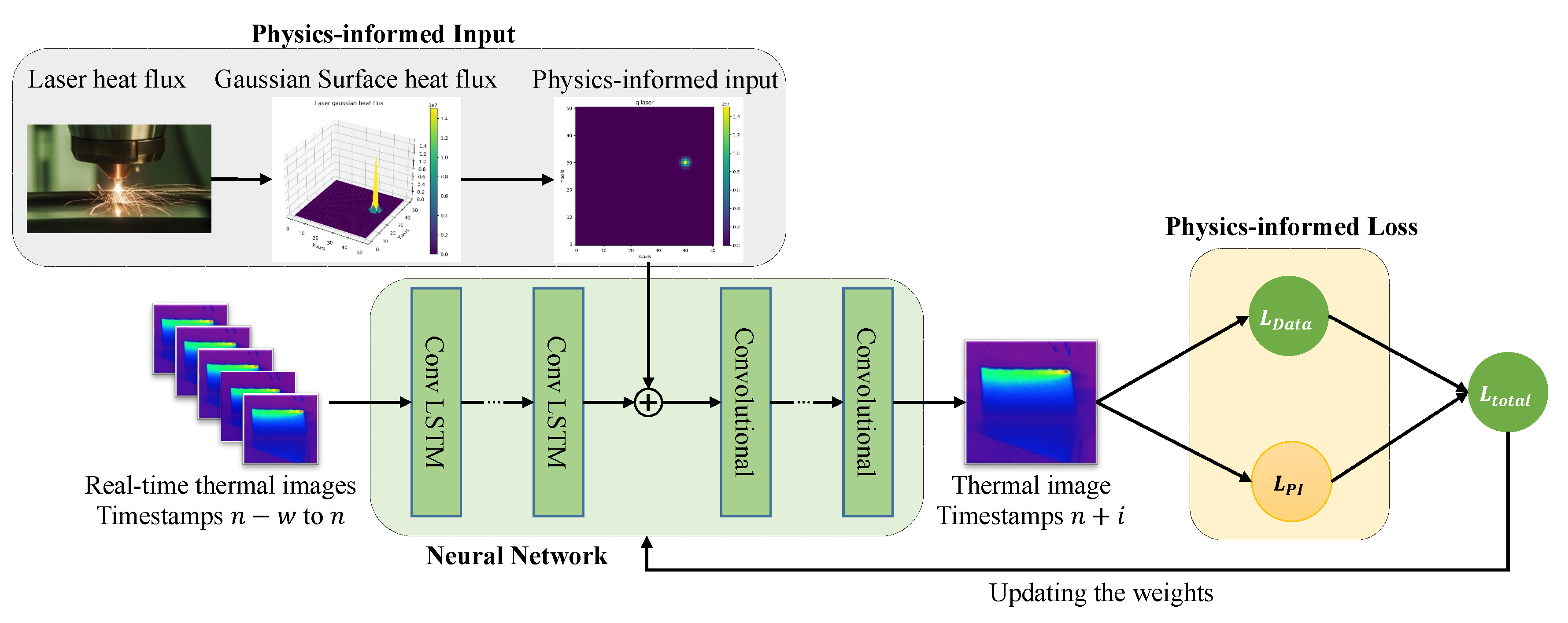
Figure 3.
An example of Gaussian surface heat flux on a surface (left) and its corresponding matrix (right)
Figure 3.
An example of Gaussian surface heat flux on a surface (left) and its corresponding matrix (right)
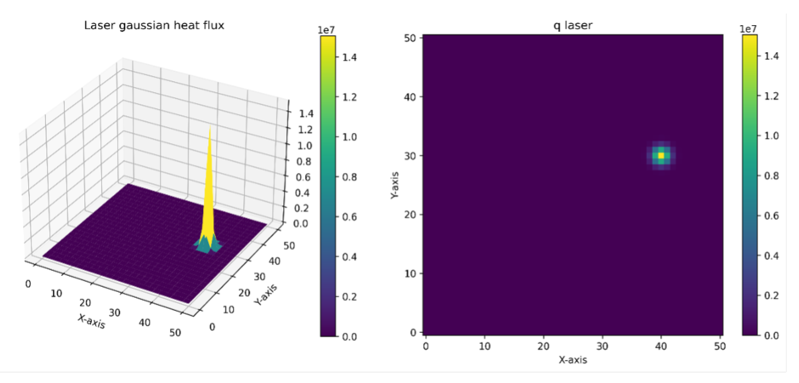
Figure 4.
Comparative Analysis of MAPE and MAE Across Processes B, C, and D
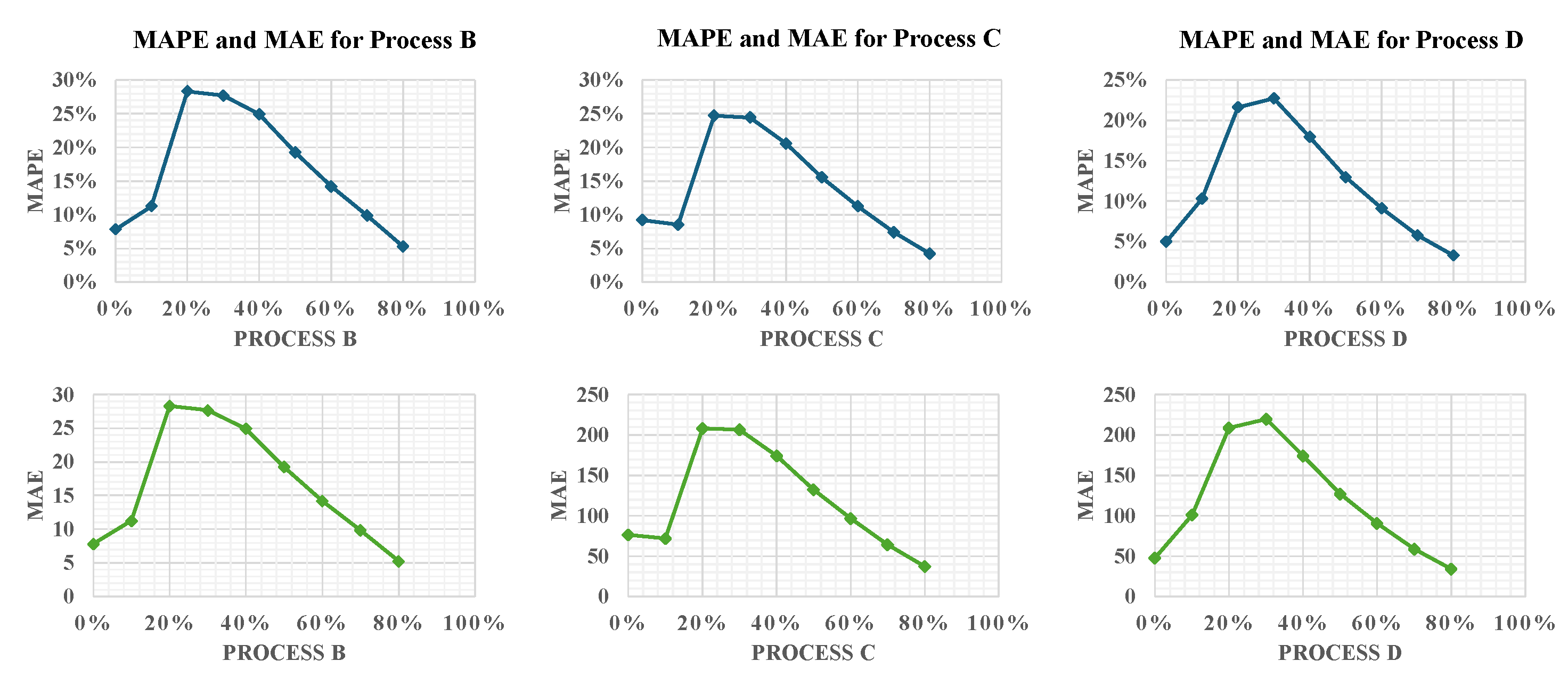
Figure 5.
Comparative MAPE of Physics-Informed and Data-Driven Models Across Processes B, C, and D
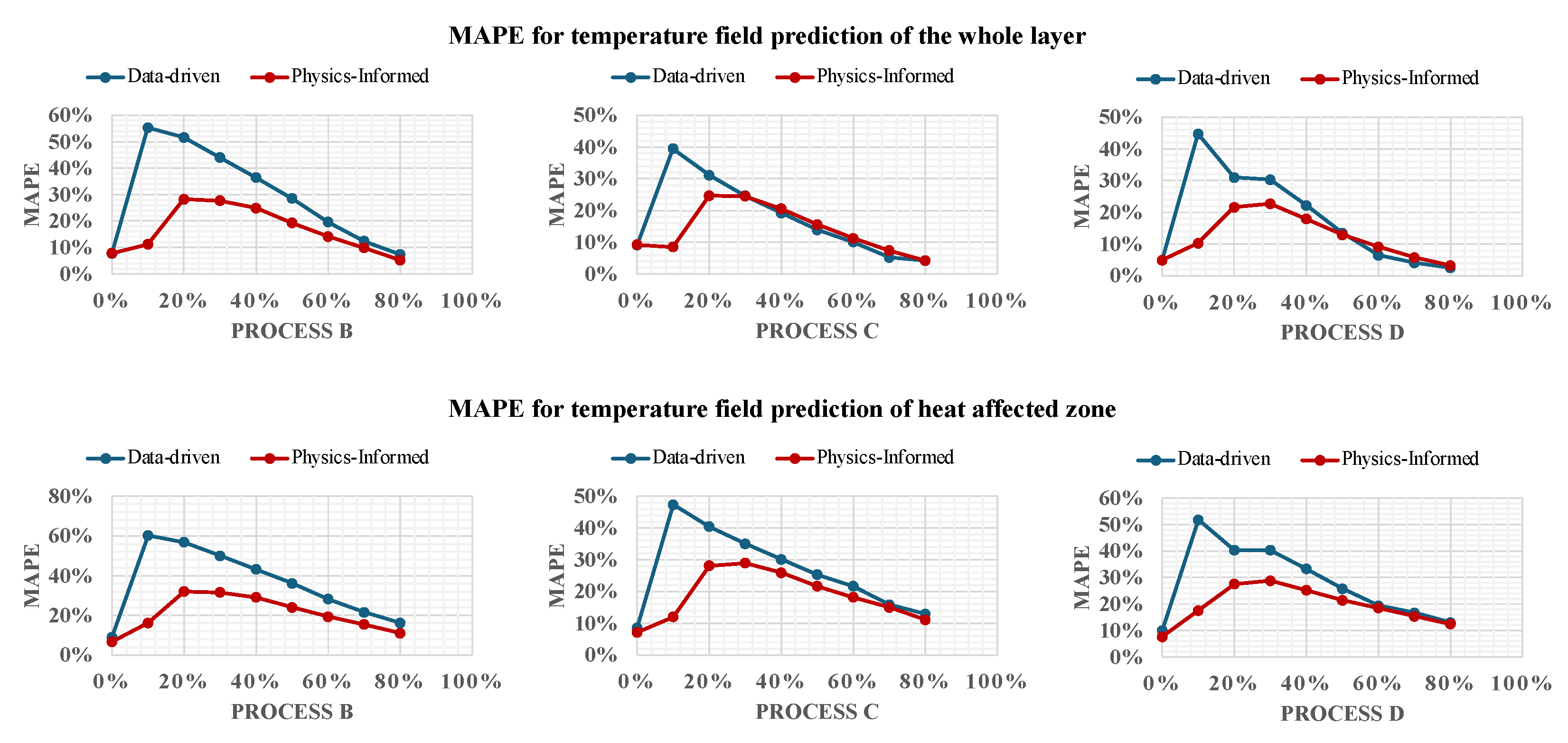
Figure 6.
Comparative Top View of Temperature Fields for Process C, Showing Framework Predictions alongside Simulation Results with Physics-Informed Predictions on Top and Data-Driven Predictions Below
Figure 6.
Comparative Top View of Temperature Fields for Process C, Showing Framework Predictions alongside Simulation Results with Physics-Informed Predictions on Top and Data-Driven Predictions Below
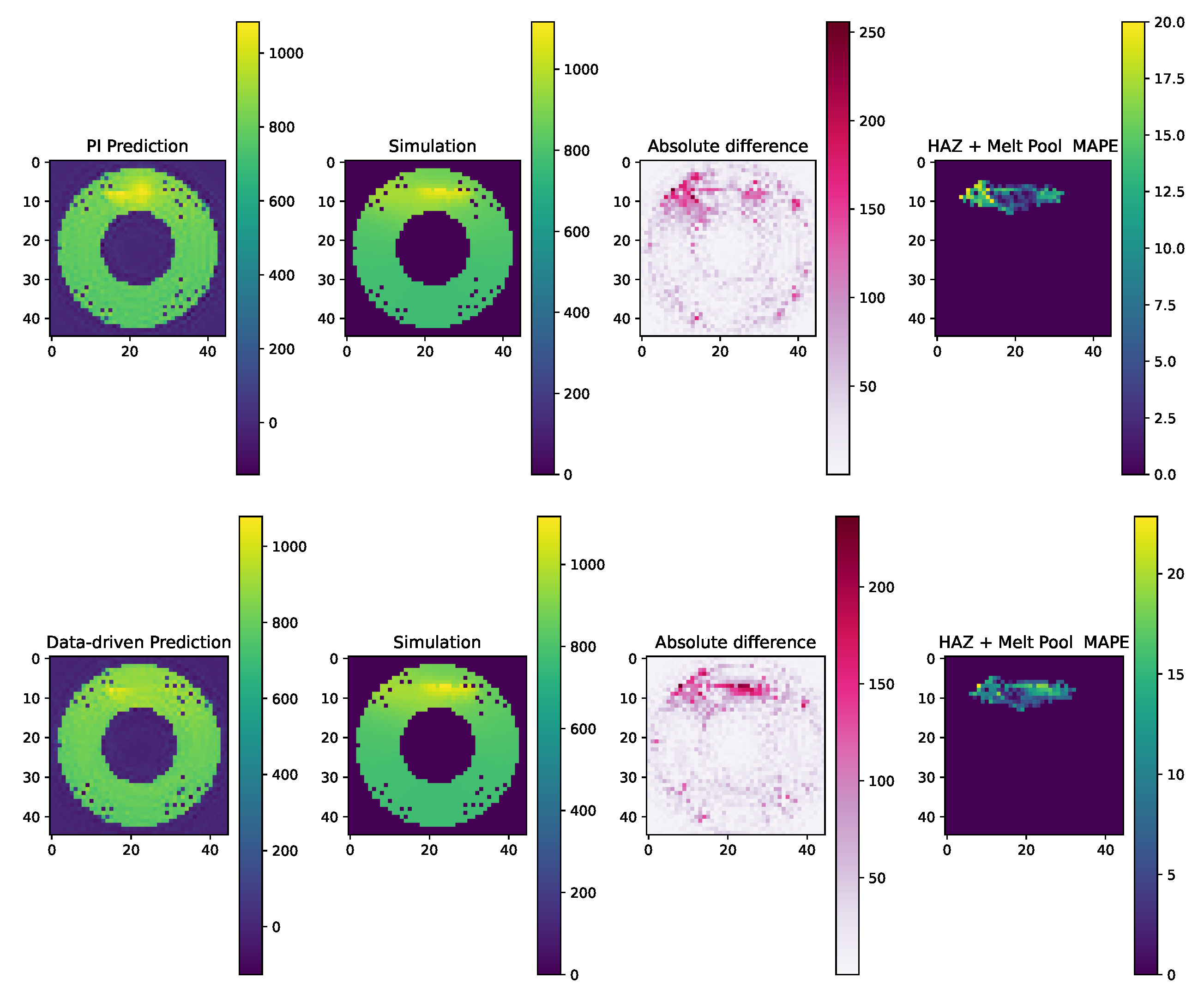
Figure 7.
Comparison of Learning Rate Strategies on PINN Performance
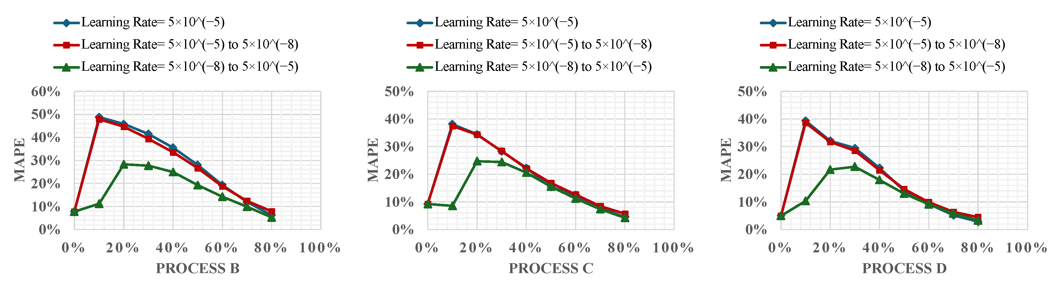
Figure 8.
Impact of Batch Size on Model Performance Across Processes B, C, and D
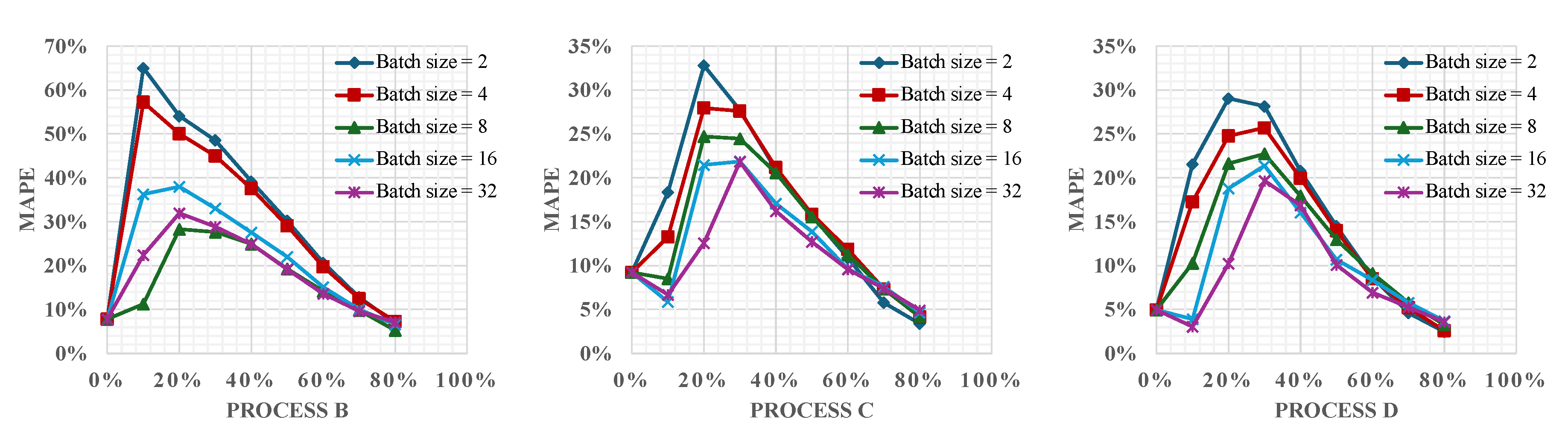

Table 1.
Illustrations of four simulated processes. In geometry and deposition patterns, the solid lines indicate the deposition geometry and the dashed lines indicate the direction of the laser scanning.
Table 1.
Illustrations of four simulated processes. In geometry and deposition patterns, the solid lines indicate the deposition geometry and the dashed lines indicate the direction of the laser scanning.
| Process A | Process B | Process C | Process D | |
|---|---|---|---|---|
| Material | 17-4PH Stainless Steel | 17-4PH Stainless Steel | 17-4PH Stainless Steel | Inconel 625 |
| Process Temperature | 2400°C | 2000°C | 2000°C | 2000°C |
| Travel Speed | 10 mm/s | 6 mm/s | 6 mm/s | 20 mm/s |
| Geometry & Deposition Pattern |  |
 |
 |
 |
Disclaimer/Publisher’s Note: The statements, opinions and data contained in all publications are solely those of the individual author(s) and contributor(s) and not of MDPI and/or the editor(s). MDPI and/or the editor(s) disclaim responsibility for any injury to people or property resulting from any ideas, methods, instructions or products referred to in the content. |
© 2024 by the authors. Licensee MDPI, Basel, Switzerland. This article is an open access article distributed under the terms and conditions of the Creative Commons Attribution (CC BY) license (http://creativecommons.org/licenses/by/4.0/).
Copyright: This open access article is published under a Creative Commons CC BY 4.0 license, which permit the free download, distribution, and reuse, provided that the author and preprint are cited in any reuse.


