
Submitted:
30 May 2024
Posted:
30 May 2024
You are already at the latest version
Abstract
This paper presents a new semi-explicit algorithm for parameters estimation in a time-fractional generalization of dual-phase-lag heat conduction model with the Caputo fractional derivatives. It is shown that this model can be derived from a general linear constitutive relation for the heat transfer by conduction when the heat conduction relaxation kernel contains the Mittag-Leffler function. The model can be used to describe heat conduction phenomena in a material with power-law memory. The proposed algorithm of parameters estimation is based on the time integral characteristics method. The explicit representations of the thermal diffusivity and the fractional analogues of the thermal relaxation time and the thermal retardation are obtained via a Laplace transform of the temperature field and utilized in the algorithm. An implicit relation is derived for the order of fractional differentiation. In the algorithm, this relation is resolved numerically. An example illustrates the proposed technique.
Keywords:
non-Fourier heat conduction model
; Caputo fractional derivative
; inverse problem
; parameters estimation
; time integral characteristic
1. Introduction
Fourier’s law is a fundamental phenomenological relation in the heat transfer theory that describes the heat conduction in solids and fluids. However, it is not applicable for modelling the heat transfer in ultrafast processes (e.g. during laser heating and cooling [1]), on micro/nanoscales (e.g. heating of carbon nanotubes [2]), in some complex media (e.g. heat conduction in biological tissues [3] and materials with non-homogeneous inner structure [4]) . For this reason, various linear and nonlinear generalizations of Fourier’s law have been proposed by many researchers through the past two centuries (see books [5,6,7] and reviews [8,9,10,11]).
The thermal conductivity is a unique property of a material in Fourier’s law whereas non-Fourier models usually include several material thermal properties. For example, the frequently used dual-phase-lag (DPL) heat conduction model, proposed by Tzou [12], incorporates the thermal conductivity, the thermal relaxation time and the thermal retardation. As a result, the possibility of using a non-Fourier model in real-world applications is based on an ability to obtain necessary thermal properties of a material. From the mathematical point of view, the problem of parameters estimation can be considered as an inverse coefficient problem which is usually ill-posed problem. Thus, the development of theoretical techniques for estimation of thermal properties in non-Fourier models is a challenging problem of mathematical modelling in the heat transfer theory.
The method of time integral characteristics (TIC) is an efficient technique for estimation of constant parameters in linear models. It was proposed by Shatalov [13] at the end of last century for solving inverse coefficient problems of heat conduction theory. The method is based on integral transformation of the initial-boundary value problem for the considered linear model on the time variable and solving the corresponding inverse coefficient problem in the transformed space. The absence of necessity to perform the inverse integral transform is a main advantage of this method. Later, this method was extended to time-fractional diffusion models [14,15].
In this study, we focus on solving the problem of parameters estimation in a time-fractional generalization of DPL heat conduction model by the method of TIC. Such model allow us to take into account power-law memory thermal effects in a material by incorporating time derivatives of fractional orders (see, e.g., [16,17]) into the thermal constitutive relation. Thus, in this model the orders of fractional differentiation are additional parameters that also have to be estimated.
Time-fractional dual-phase-lag (TFDPL) model was proposed by Xu and Jiang [18] to interpret the experiment results for processed meat. The Caputo time-fractional derivatives of two different orders are used in this model. The authors obtained analytical solution of the corresponding bioheat transfer equation and solved the inverse problem for estimation of model parameters by applying the nonlinear least-square method. The same model was used in [19] for treating thermoelastic response of skin subjected to sudden temperature shock. In [20], a fundamental solution of the TFDPL heat conduction problem was obtained. Also, a TFDPL model with a single order of fractional differentiation was considered by several scholars. In [21], such a model was used for describing the heat conduction in a multi-layered spherical medium with azimuthal symmetry. In [22], a similar model with temperature jump boundary condition was utilized for numerical simulation of heat transfer in transistors. Numerical schemes for solving several TFDPL heat conduction problems was proposed in [23,24].
However, it is necessary to note that in all papers mentioned above the considered TFDPL models have been obtained from the classical DPL model by formal replacing of the integer order time derivatives by their fractional analogues. In this paper we overcome this weakness by proposing the derivation of TFDPL model from a general linear constitutive relation for the heat transfer by conduction.
The paper is organized as follows. Section 2 contains a brief description of the time integral characteristic method. Section 3 is devoted to derivation of the TFDPL heat conduction model and corresponding non-Fourier heat conduction equation. A proposed semi-explicit algorithm for TFDPL model parameters estimation is described in Section 4. An illustrative example of using this algorithm is presented in Section 5.
2. Preliminaries
This section gives a brief description of the TIC method. This method was proposed for solving inverse problems of parameters estimation in linear evolution equations.
Let us illustrate the basic idea of the TIC method by a simple problem of the thermal diffusivity estimation. We consider the heat equation
Here x and t are spatial and temporal variables, respectively, is the temperature field, a is the thermal diffusivity. This equation is accompanied with the initial condition
the boundary conditions
and the additional internal condition
Here , are known functions. Then the inverse coefficient problem is stated as follows: given the initial boundary value problem (1), (2), (3) and the additional condition (4), find the constant thermal diffusivity a.
The method of TIC is based on an integral transformation of the temperature field with respect to time. The Laplace transform
can be efficiently used for this purpose. The function is referred to as a time integral characteristic of the temperature field T at the point .
The initial boundary value problem (1), (2), (3) after Laplace transformation takes the form
and (4) gives
In (6), prime denotes differentiation with respect to x.
Then, by using (8), we find the following explicit representation of the thermal diffusivity via TICs of the temperature field:
A main advantage of the described technique is that there is no necessity to perform the inverse Laplace transform. If the temperature functions and are known exactly, the representation (9) gives the exact value of a for all permitted values of p. However, in practice such functions are usually measured in an experiment with some errors. Then the Laplace parameter p should be considered as a regularization parameter and its value should be chosen in agreement with experimental errors. The explicit representation (9) permits to obtain a linear estimate of relative error for the thermal diffusivity as a function of p (see [13,14,15] for more details). The minimum of this function gives the optimal value of p.
3. The time-fractional dual-phase-lag heat equation
A TFDPL heat conduction model can be obtained similarly to the time-fractional Zener model in the theory of linear fractional viscoelasticity [25].
A general linear constitutive relation for the heat transfer by conduction in homogeneous and isotropic materials with memory is defined mathematically using a Riemann–Stieltjes integral as
Here is the heat flux vector, is the temperature gradient, and is the heat conduction relaxation function which does not depend on the spatial coordinate .
In accordance to the physical principle of causality, the relaxation function is zero for negative time. Hence, the constitutive relation (10) takes the form
It is easy to see that this equation reduces to Fourier’s law if and where k is the thermal conductivity which is a constant in time.
Assuming that and are continuous functions, we can rewrite (11) in a more convenient form
Let us now consider the case when the heat conduction relaxation function has the form
where are constants and
is the Mittag-Leffler function (see, e.g., [17]). This function has the known property
i.e. it is invariant with respect to the left-sided Caputo fractional derivative of order . This fractional derivative reads
Here is the left-sided fractional integral operator of order . Letting in (16), we obtain the Caputo fractional operator for the whole axis . Applying this operator to both sides of (12), we get
We assume here that is a <<sufficiently good>> function so that all integrals exist. Changing the order of integration in the last term of the above expression, we obtain
It is easy to see that integrals in the last terms of (18) and (19) coincide and therefore can be excluded. As a result, we obtain the time-fractional constitutive relation
Using the definition of the function , this relation can be written as
Here is the thermal conductivity, is the fractional analogue of the thermal relaxation time (the so-called phase lag in the heat flux), and is the fractional analogue of the thermal retardation (the so-called temperature gradient phase lag).
The constitutive relation (20) describes the heat conduction in a material with full power-law memory. This relation is invariant with respect to translation in time and therefore the time origin can be arbitrarily chosen.
Let us now assume that there is not heat transfer in a material for time . Then the relation (20) reduces to
Note that this relation is not invariant with respect to translation in time and the time origin is fixed in this case.
Now we can obtain TFDPL heat equation. The energy conservation law for a constant property material without heat sources can be written as
where c is the specific heat and is the density of material. Combining (21) and (22), after simple algebra, we get
where is the thermal diffusivity. TFDPL heat equation (22) models heat conduction in a material with power-law memory and constant temperature field for time .
4. An Algorithm of TFDPL Model Parameters Estimation
Let us consider a one-dimensional case of TFDPL heat equation (23) in a half space, namely
This is a time-fractional equation of order and therefore two initial conditions are needed for its unique solvability. We take them in the form
where is a constant initial temperature.
We will also assume that (24) is accompanied by the boundary conditions
and by the additional internal condition
Here , are known functions.
We will consider the following inverse problem: given the initial boundary value problem (24), (25), (26) and the additional condition (27), find the constants a, , , . For solving this problem, the method of TIC can be efficiently used.
Here the functions and are known.
The initial-boundary problem (28), (29), (30) after Laplace transform can be written as
and (31) gives
Here denotes the Laplace transform of which is defined by
In (32), prime denotes differentiation with respect to x.
Using the additional condition (34), we get the main equation for parameters estimation which can be written as
where
Note that the function is linear with respect to a, b, , and nonlinear with respect to .
As it was mentioned in Preliminaries section, the problem of finding the Laplace parameter p arises if the functions and are not known exactly. In the method of TIC, the Laplace parameter p is assumed to be real and positive. Therefore, it is naturally to assume that this parameter belongs to a finite interval . A discussion of different approaches to estimation of and can be found in [14,15]. Then the considered inverse problem can be reduced to minimization problem
This is a classical problem of finding a minimum of four variables function f. The physical constraints are , , , and . In general, this problem can be solved numerically by using different optimization software.
However, explicit TIC representations for desired parameters can be obtained in a special case when the order of fractional differentiation is known. Let us consider (37) as unconstrained minimization problem. It is obvious that the function f defined by (37) is a quadratic function in three variables a, b and . The necessary conditions for local optimality reads
These conditions give the system of linear equations
where
and
Note that the matrix A is symmetric.
Using Cramer’s rule, the solution of (38) can be written in the explicit form
where
and is the matrix formed by replacing the i-th column of A by the column vector B. Thus, the explicit representations (39) permit to obtain the values of a, b and for a given value of .
In (40), the parameters a, b and are the functions of which are defined by (39). We thus obtain a single equation for . The equation (40) is nonlinear and quite complex. Therefore, it should be solved numerically.
As a result, we can state the following semi-explicit algorithm for parameters estimation in TFDPL heat conduction model:
It is necessary to note that the proposed algorithm is based on the unconstrained minimization problem. As a result, the order of fractional differentiation which is obtained as the solution of (40) is not necessary belong to the interval . Then the constrained minimization problem mentioned above should be considered and solved numerically. Note that usually this situation arises when the initial functions and have quite large errors (usually more than 5 %).
The considered problem of parameters estimation belongs to the class of inverse coefficient problems. Hence, it is an ill-posed problem in most cases. In the proposed algorithm, the stabilization of solution is achieved by integration with respect to the Laplace parameter p. However, numerical experiments show that the solution is stable only if with . If , the determinant is close to zero and corresponding approximate solution is unstable. An additional regularization is needed in this case. For example, the Tikhonov regularization method can be used for this purpose.
5. An Example
To illustrate the above algorithm, let us consider the equation (28) with
Hence, and
Three different values of fractional order are considered: , and . The graphs of the function defined by (41) for these values of are shown in Figure 1.
Denote by and the exact and perturbed temperature fields, respectively. Let
where is the upper error bound. Then it is easy to prove (see, e.g., [13]) that
Thus, the error of is increased as the parameter p is decreased. The same is valid for the function .
To simulate experimental errors, we approximated the function on the interval by polynomials of different degrees with respect to a new dependent variable
The values of and were used in all numerical calculations. Also, we utilized the relative error as a metric of accuracy. For a quantity q, it is defined by
where and are exact and perturbed values of q, respectively.
Case 1: .
The following approximations of were constructed:
The graphs of relative errors for these functions are plotted in Figure 2. It can be seen that the maximum value of relative error is approximately equal to for , for , and for .
Table 1 contains the results of parameters estimation by using the explicit expressions given in (39) for and approximate functions from (42). Note that in this case . It can be seen that the relative errors of a and b are of the same order of magnitude as the corresponding relative errors of functions . The relative errors of and are also in good agreement with the relative errors of and . However, in the case of quite large initial error when the function is used, the error level of and is highly increased.
Table 2 contains the results of parameters estimation for unknown . In this case the equation (40) was solved for each (). As can be seen from the table, the accuracy of identification is highly depends on error of initial data. The same is valid for other parameters.
Case 2: .
The following approximations of were obtained:
The graphs of relative errors for these functions are plotted in Figure 3. The maximum value of relative error is approximately equal to for , for , and for .
The results of parameters estimation are given in Table 3 for , and in Table 4 for initially unknown . In general, the results of this case are close to previous one. However, the magnitudes of relative errors for estimated parameters are greater than those obtained previously. This is because in this case.
Case 3: .
In this case, the following approximations of were constructed:
The graphs of relative errors for the functions in (44) are plotted in Figure 4. The maximum value of relative error is approximately equal to for , for , and for .
Table 5 contains the results of parameters estimation by using (39) for and approximations (44). In this case we found and therefore the estimation results are highly sensitive to errors of initial data. It follows from the table that if we use function having relative error at most , the proposed algorithm does not permit to identify with the chosen values of and . However, we obtained reasonable values of all desired parameters for the function . This demonstrates the stability of the algorithm.
Finally, Table 2 contains table 6 citatin, table 6 is not cited. the results of parameters estimation for unknown . It can be seen from the table that in all cases we have a high level of error, especially for .
Thus, we can conclude that the proposed algorithm permits to estimate the parameters of TFDPL model with a reasonable accuracy if with . For fixed values of and , decreasing of leads to decreasing of . Hence, the values of and should be chosen dependently on . Also, it should be pointed out that the parameters and are more sensitive to error level in initial data than a and .
Author Contributions
Not applicable.
Funding
This research received no external funding.
Institutional Review Board Statement
Not applicable.
Informed Consent Statement
Not applicable.
Data Availability Statement
Not applicable.
Abbreviations
The following abbreviations are used in this manuscript:
| DPL | Dual-phase-lag |
| TFDPL | Time-fractional dual-phase-lag |
| TIC | Time integral characteristic |
References
- Qiu, T.Q.; Tien, C.L. Heat Transfer Mechanisms During Short-Pulse Laser Heating of Metals. J. Heat Transfer 1993, 115(4), 835–841. [Google Scholar] [CrossRef]
- Wang, H.D.; Cao, B.Y.; Guo, Z.Y. Non-Fourier Heat Conduction in Carbon Nanotubes. J. Heat Transfer 2012, 134(5), 051004. [Google Scholar] [CrossRef]
- Askarizadeh, H.; Ahmadikia, H. Analytical study on the transient heating of a two-dimensional skin tissue using parabolic and hyperbolic bioheat transfer equations. Appl. Math. Model. 2015, 39(13), 3704–3720. [Google Scholar] [CrossRef]
- Roetzel, W.; Putra, N.; Das, S.K. Experiment and analysis for non-Fourier conduction in materials with non-homogeneous inner structure. Int. J. Therm. Sci. 2003, 42(6), 541–552. [Google Scholar] [CrossRef]
- Wang, H-D. Theoretical and Experimental Studies on Non-Fourier Heat Conduction Based on Thermomass Theory; Springer: Berlin, Germany, 2014. [Google Scholar]
- Dong, Y. Dynamical Analysis of Non-Fourier Heat Conduction and Its Application in Nanosystems; Springer: Berlin, Germany, 2016. [Google Scholar]
- Zhmakin, A.I. Non-Fourier Heat Conduction: From Phase-Lag Models to Relativistic and Quantum Transport; Springer Cham, 2023.
- Wang, F.F.; Wang, B. Current Research Progress in Non-Classical Fourier Heat Conduction. Applied Mechanics and Materials 2013, 442, 187–196. [Google Scholar] [CrossRef]
- Zhmakin, A.I. Heat Conduction Beyond the Fourier Law. Tech. Phys. 2021, 66, 1–22. [Google Scholar] [CrossRef]
- Khayat, R.E.; deBruyn, J.; Niknami, M.; et al. Non-Fourier effects in macro- and micro-scale non-isothermal flow of liquids and gases. Review. Int. J. Therm. Sci. 2015, 97, 163–177. [Google Scholar] [CrossRef]
- Benenti, G.; Donadio, D.; Lepri, S.; et al. Non-Fourier heat transport in nanosystems. Riv. Nuovo Cim. 2023, 46, 105–161. [Google Scholar] [CrossRef]
- Tzou, D.Y. A unified approach for heat conduction from macro to micro-scales. ASME J. Heat Transfer, 1995, 117, 8–16. [Google Scholar] [CrossRef]
- Shatalov, Yu.S. Integral Representation of Constant Heat Transfer Coefficients Publ.of Ufa Aviation Institute, Ufa, Russia, 1992. (in Russian).
- Lukashchuk, S.Yu. Estimation of parameters in fractional subdiffusion equations by the time integral characteristics method. Comput. Math. Appl. 2011, 62(3), 834–844. [Google Scholar] [CrossRef]
- Lukashchuk, S.Yu. Approximation of ordinary fractional differential equations by differential equations with a small parameter. Vestn. Udmurtsk. Univ. Mat. Mekh. Komp. Nauki 2017, 27, 515–531. [Google Scholar] [CrossRef]
- Samko, S.; Kilbas, A.; Marichev, O. Fractional Integrals and Derivatives. Theory and Applications; Gordon & Breach Sci. Publishers: London, UK, 1993. [Google Scholar]
- Kilbas, A.A.; Srivastava, H.M.; Trujillo, J.J. Theory and Applications of Fractional Differential Equations; Elsevier: Amsterdam, The Netherlands, 2006. [Google Scholar]
- Xu, H.-Y.; Jiang, X.-Y. Time fractional dual-phase-lag heat conduction equation. Chin. Phys. B 2015, 24(3), 034401. [Google Scholar] [CrossRef]
- Chaudhary, R.K.; Singh, J. Numerical simulation of non–linear skin model with energy dissipation during hyperthermia and its validation with experimental data. J. Therm. Stresses 2024, 47(1), 80–98. [Google Scholar] [CrossRef]
- Ciesielski, M.; Siedlecka, U. Fractional Dual-Phase Lag Equation—Fundamental Solution of the Cauchy Problem. Symmetry 2021, 13, 1333. [Google Scholar] [CrossRef]
- Kukla, S.; Siedlecka, U.; Ciesielski, M. Fractional Order Dual-Phase-Lag Model of Heat Conduction in a Composite Spherical Medium. Materials 2022, 15, 7251. [Google Scholar] [CrossRef] [PubMed]
- Fotovvat, M.H.; Shomali, Z. A time-fractional dual-phase-lag framework to investigate transistors with TMTC channels (TiS3, In4Se3) and size-dependent properties. Micro and Nanostructures 2022, 168, 207304. [Google Scholar] [CrossRef]
- Ji, C.-c.; Dai, W.; Sun, Z.-z. Numerical Method for Solving the Time-Fractional Dual-Phase-Lagging Heat Conduction Equation with the Temperature-Jump Boundary Condition. J. Sci. Comput. 2018, 75(3), 1307–1336. [Google Scholar] [CrossRef]
- Ji, C.-c.; Dai, W.; Sun, Z.-z. Numerical Schemes for Solving the Time-Fractional Dual-Phase-Lagging Heat Conduction Model in a Double-Layered Nanoscale Thin Film. J. Sci. Comput. 2019, 81(3), 1767–1800. [Google Scholar] [CrossRef]
- Mainardi, F. Fractional calculus and waves in linear viscoelasticity, Imperial College Press: London, UK, 2010.
Figure 1.
The graphs of the function defined by (41) for different values of .
Figure 1.
The graphs of the function defined by (41) for different values of .
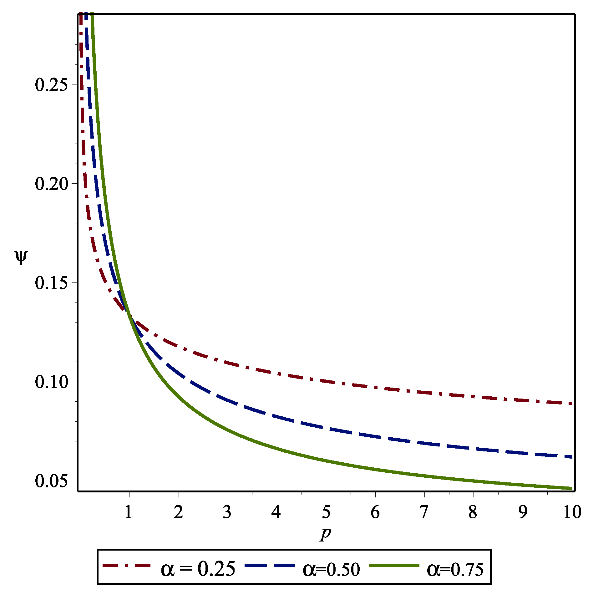
Figure 2.
The graphs of relative errors for functions (42).
Figure 2.
The graphs of relative errors for functions (42).
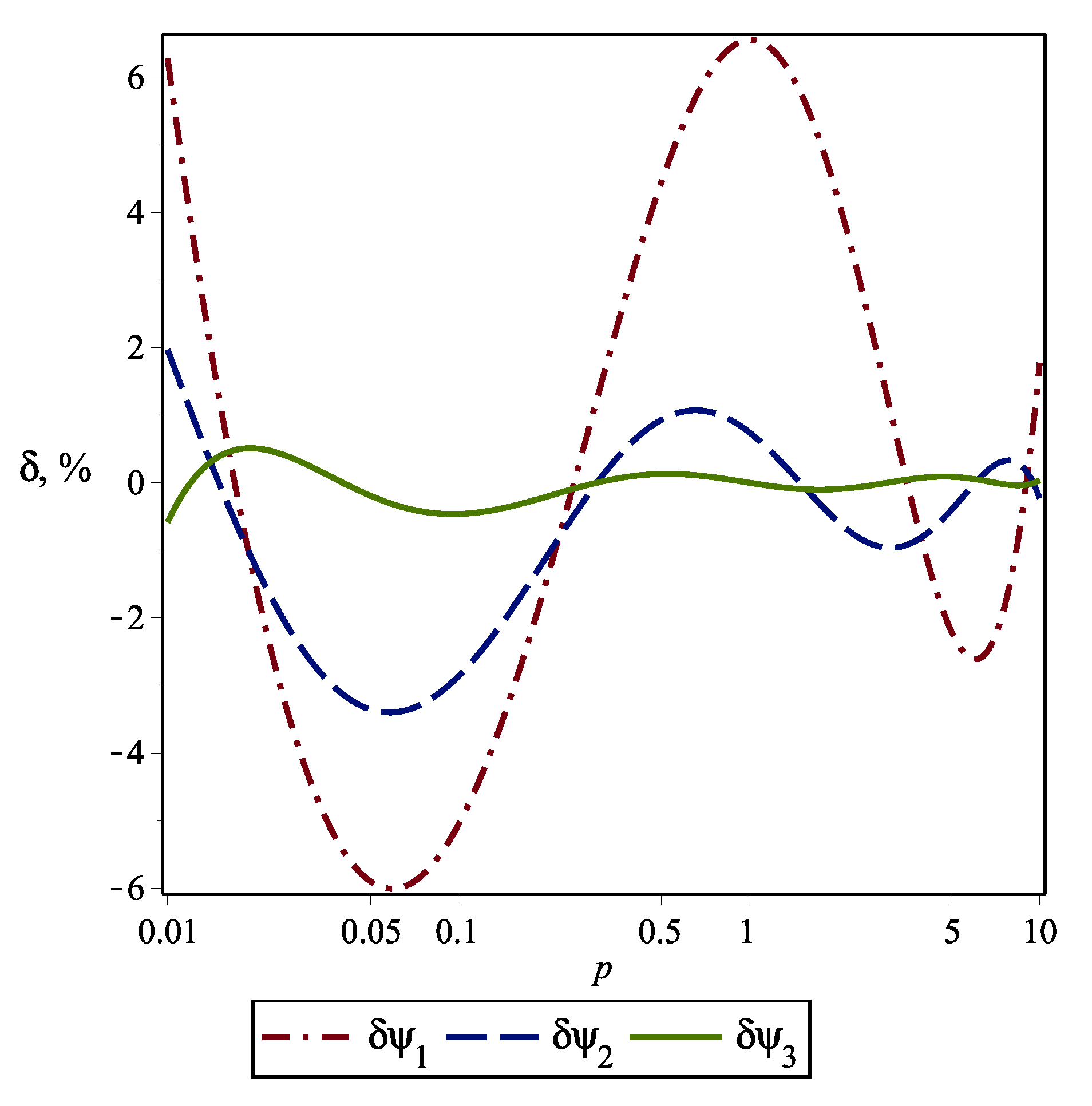
Figure 3.
The graphs of relative errors for functions (43).
Figure 3.
The graphs of relative errors for functions (43).
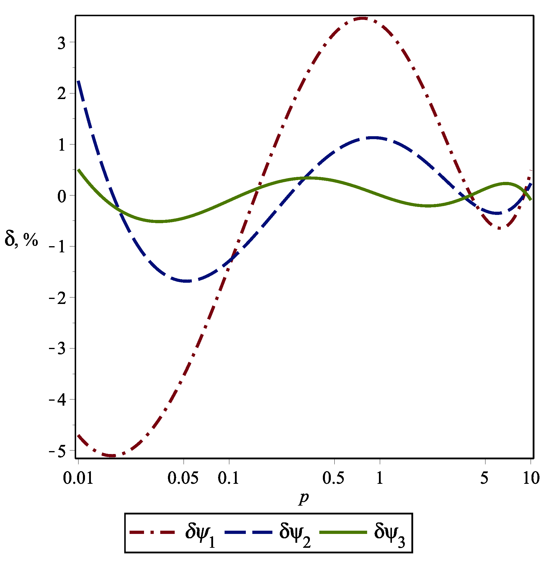
Figure 4.
The graphs of relative errors for functions (44).
Figure 4.
The graphs of relative errors for functions (44).
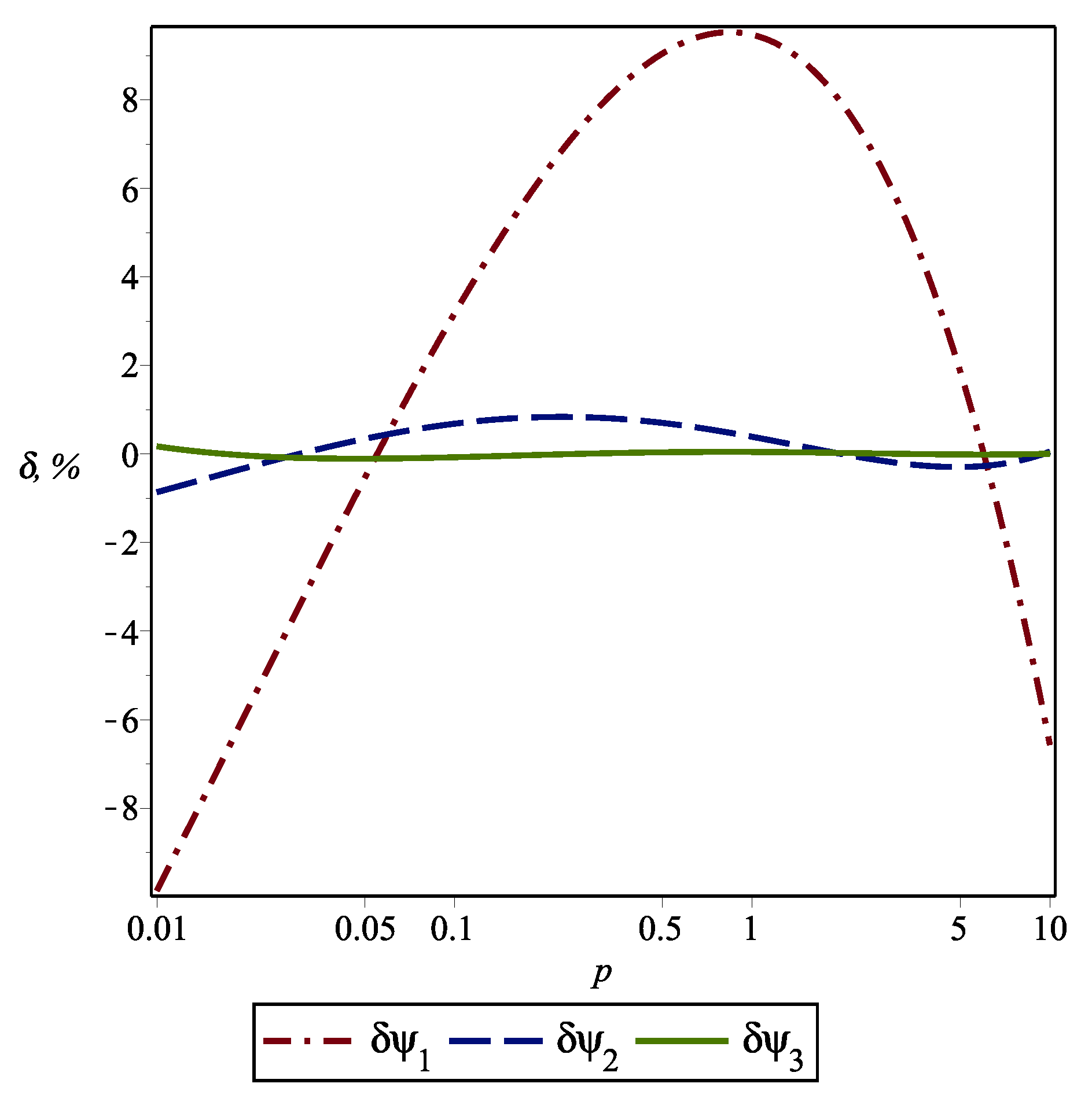

Table 1.
Comparison of the restored parameters for different approximations of with .
| error (%) | error (%) | error (%) | ||||
|---|---|---|---|---|---|---|
| a | 1.0042 | 0.42 | 1.0072 | 0.72 | 1.0700 | 7.00 |
| b | 8.0269 | 0.34 | 8.0591 | 0.74 | 7.4649 | 6.70 |
| 7.9933 | 0.08 | 8.0015 | 0.02 | 6.9765 | 12.8 | |
| 0.1997 | 0.15 | 0.2031 | 1.55 | 0.1664 | 16.8 |
Table 2.
Comparison of the restored parameters for different approximations of with .
| error (%) | error (%) | error (%) | ||||
|---|---|---|---|---|---|---|
| 0.7479 | 0.28 | 0.7831 | 4.41 | 0.8606 | 14.7 | |
| a | 0.9968 | 0.32 | 1.1264 | 12.6 | 1.4314 | 43.1 |
| b | 7.9981 | 0.02 | 7.9802 | 0.25 | 7.1442 | 10.7 |
| 8.0238 | 0.30 | 7.0847 | 11.4 | 4.9912 | 37.6 | |
| 0.1990 | 0.50 | 0.2139 | 6.95 | 0.1978 | 1.10 |
Table 3.
Comparison of the restored parameters for different approximations of with .
| error (%) | error (%) | error (%) | ||||
|---|---|---|---|---|---|---|
| a | 0.9893 | 1.07 | 1.0530 | 5.30 | 1.1456 | 14.6 |
| b | 8.0371 | 0.46 | 7.7986 | 2.52 | 7.3658 | 7.93 |
| 8.1242 | 1.55 | 7.4060 | 7.43 | 6.4296 | 19.6 | |
| 0.2029 | 1.45 | 0.1867 | 6.65 | 0.1588 | 20.6 |
Table 4.
Comparison of the restored parameters for different approximations of with .
| error (%) | error (%) | error (%) | ||||
|---|---|---|---|---|---|---|
| 0.5058 | 1.16 | 0.5249 | 4.98 | 0.5932 | 18.6 | |
| a | 1.0262 | 2.62 | 1.2017 | 20.2 | 1.6321 | 63.2 |
| b | 8.0298 | 0.37 | 7.7744 | 2.82 | 7.2866 | 8.92 |
| 7.8247 | 2.19 | 6.4693 | 19.1 | 4.4645 | 44.2 | |
| 0.2073 | 3.65 | 0.2052 | 2.60 | 0.2214 | 10.7 |
Table 5.
Comparison of the restored parameters for different approximations of with .
| error (%) | error (%) | error (%) | ||||
|---|---|---|---|---|---|---|
| a | 1.0117 | 1.17 | 0.9273 | 7.27 | 2.7387 | 174 |
| b | 7.9691 | 0.39 | 8.0479 | 0.60 | 2.6336 | 67.1 |
| 7.8770 | 1.54 | 8.6791 | 8.49 | 0.9616 | 88.0 | |
| 0.1977 | 1.15 | 0.1988 | 0.60 | -0.2138 | — |
Table 6.
Comparison of the restored parameters for different approximations of with .
| error (%) | error (%) | error (%) | ||||
|---|---|---|---|---|---|---|
| 0.2541 | 1.64 | 0.3299 | 32.0 | 0.0187 | 92.5 | |
| a | 1.0706 | 7.06 | 1.8943 | 89.4 | 0.3296 | 67.0 |
| b | 7.9662 | 0.42 | 7.9957 | 0.05 | 0.3262 | 95.9 |
| 7.4411 | 6.99 | 4.2208 | 47.2 | 0.9896 | 87.6 | |
| 0.2953 | 47.7 | 0.3227 | 61.4 | -0.9045 | — |
Disclaimer/Publisher’s Note: The statements, opinions and data contained in all publications are solely those of the individual author(s) and contributor(s) and not of MDPI and/or the editor(s). MDPI and/or the editor(s) disclaim responsibility for any injury to people or property resulting from any ideas, methods, instructions or products referred to in the content. |
© 2024 by the authors. Licensee MDPI, Basel, Switzerland. This article is an open access article distributed under the terms and conditions of the Creative Commons Attribution (CC BY) license (http://creativecommons.org/licenses/by/4.0/).
Copyright: This open access article is published under a Creative Commons CC BY 4.0 license, which permit the free download, distribution, and reuse, provided that the author and preprint are cited in any reuse.


