
Submitted:
21 May 2024
Posted:
21 May 2024
You are already at the latest version
Abstract
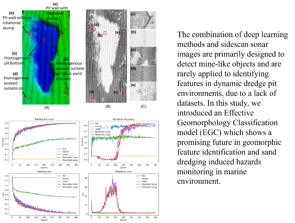
Deep learning methods paired with sidescan sonar (SSS) are commonly used in underwater search and rescue operations for drowning victims, wrecks, and airplanes. However, these techniques are primarily designed to detect mine-like objects and are rarely applied to identifying features in dynamic dredge pit environments, due to a lack of datasets. In this study, we present a Sandy Point Dredge Pit (SPDP) dataset, in which high-resolution SSS data were collected from the west flank of Mississippi bird foot delta of the Louisiana inner shelf. This dataset contains a total of 385 SSS images. We introduce an Effective Geomorphology Classification model (EGC). By ablation studies, we analyze the utility of transfer learning on different model architectures and the impact of data augmentations on model performance. This EGC model will make geomorphic features identification in dredge pit environments quick and efficient which requires extensive experience and professional knowledge. The combination of SSS images and EGC model is a cost-effective and valuable toolkit for hazards monitoring in marine dredge pit environment. The SPDP SSS images dataset, especially the feature of pit wall without rotational slump, is also valuable for other machine learning modelers.
Keywords:
sidescan
; sonar
; geomorphology
; deep learning
; coastal restoration
; EfficientNet
1. Introduction
Barrier islands play a critical role in safeguarding inland wetlands and preserving estuarine conditions [1]. The barrier islands within the Mississippi River delta plain are facing rapid deterioration due to a combination of factors including significant relative sea-level rise of approximately 0.9 cm/year, a shortage of coastal sand supply, and erosion from storm-induced waves and currents ([2,3,4,5]). These challenges have been documented extensively in research over the past decades, highlighting the islands' vulnerability and the pressing need for conservation efforts ([6,7,8]).
Dredging, recognized globally as a critical excavation activity, entails the extraction and transfer of sediments from the beds of oceans, rivers, and lakes. This process serves multiple purposes, ranging from the creation and enhancement of maritime infrastructures such as harbors, waterways, and dikes, to land reclamation efforts. Additionally, dredging is integral to flood and storm mitigation, the harvesting of minerals for infrastructure projects, and the remediation of contaminated sediments. This is detailed in various studies, including those by [9,10,11,12,13,14]. Specifically dredging activities on the inner Louisiana continental shelf are of notable economic and societal importance, with over 50,000 km of pipelines on the Gulf of Mexico's seabed. The Energy Information Administration highlights the Gulf of Mexico's (GOM) substantial contribution to the U.S.'s offshore oil and natural gas production, alongside its pivotal role in housing a significant portion of the country’s petroleum refining and natural gas processing capacities. Therefore, landslide monitoring is significant for sediment and energy management.
Synthesizing historical data and continuously monitoring the pits have been an interest of mineral resource managers and decision makers ([15,16,17,18,19]). Conventional approaches to analyzing pre-dredging, dredging, and post-dredging phases incorporate a variety of techniques, such as geophysical surveys (including bathymetric, subbottom, and sidescan), sediment sampling through corings and grabs, water analysis, and continuous monitoring with optical and acoustic sensors ([20,21]). These methods are complemented by profiling, ship-based transects, among others. While coring and geophysical surveys are effective in identifying sediment characteristics, they often come with limitations regarding spatial coverage and high costs. Sediment coring, although accurate for groundtruthing conditions on the ground, is notably time-intensive and requires significant labor, typically executed intermittently over extended periods (for example, during seasonal studies) ([22]). Multi-beam bathymetric surveys offer detailed insights into morphological changes but are expensive, leading to infrequent monitoring of many dredge sites, possibly only once every few years ([20,23,24]). In contrast, side-scan sonar, with its broader survey range, stands out as a potential cost-effective method for identifying various sediment substrates, including rocky terrains, wrecks, oyster beds, sand, and mud, demonstrating its versatility and efficiency in marine substrate detection ([20,25,26]).
Machine Learning (ML) has emerged as a pivotal technology in the enhancement of feature identification within side scan sonar imagery, a critical tool for underwater exploration, including seabed types, marine habitats, archaeological sites, and man-made objects like shipwrecks and debris, and monitoring ([27,28,29]). [30] discussed SSS image augmentation for sediment classification. Their results indicate that pre-trained EfficientNet model improve accuracy after fine tuning the parameter in feature identification and object classification using SSS images. [31] confirmed that the segmentation method based on conventional neural networks (CNN) and Markov random fields (MRF) is applicable in SSS image segmentation. [32] combined semisynthetic data generation and deep transfer learning which has proved to be an effective way to improve the accuracy of underwater object classification. [33] presented textural analyses of SSS images from Stanton Banks, on the continental shelf off Northen Ireland. They detected faint trawling marks and separated between the different types of seafloors. [34] discussed an automated pipeline for identifying sites of archaeological interests off the coast of Malta from SSS images collected by an autonomous underwater vehicle (AUV). Their algorithm achieves precision and recall, up to 29.34% and 97.22%. Based on the above literature review, the main contributions and work of this paper are given as follows.
- 1)
- This automation significantly improves the efficiency and accuracy of SSS image analysis, overcoming the traditional challenges of manual interpretation, which is time-consuming and subject to human error in the dredge pit sedimentary environment.
- 2)
- Pit wall collapse could threaten the safety of ambient pipelines and platforms. The combination of EGC model and SSS images is a promising tool for future dredge pit geomorphic feature evolution and hazards related to dredging.
- 3)
- As the first dredge pit wall collapse SSS images, it could be used in other environment for the hazard monitoring.
2. Sandy Point Dredge Pit Dataset and Effective Geomorphology Classification Model
2.1. Sandy Point Dredge Pit Dataset
In this section, we first introduce the interest of area. Then the data collection process will be introduced, and multiple data augmentation techniques used for the training of deep learning models are presented.
2.1.1. Study Area
The Sandy Point dredge pit, situated 20 km west of the modern Mississippi River bird-foot delta, reaches a depth of about 20 m post-dredging, contrasted with the surrounding water's depth of approximately 11 m (Figure 1). This pit originated from an ancient sandy paleo river channel covered extensively by muddy deposits [7]. The nearby fluvial deposits from Grand Pass of the Mississippi Delta, about 12.5 km northeast of the pit, influence its shape and dynamics significantly. Over time, sediment dispersal from the Mississippi River has led to a seabed predominantly composed of mud around the Sandy Point pit area. Specifically, the bottom sediment composition here is 90% mud (particles finer than 63 μm) and 10% sand, contributing to its unique characteristics [7].
2.1.2. Data Collection
To collect Sandy Point Dredge Pit (SPDP) dataset, we surveyed the Sandy Point dredge pit in September 2022 using a full suite of high-resolution geophysical instruments, including interferometric sonar for swath bathymetry, sidescan sonar, and CHIRP subbottom profiler. The 4600 system produces real-time high-resolution three-dimensional maps of the seafloor while providing co-registered simultaneous sidescan and bathymetric data. Seafloor features, such as pit edges, failure scarps, and bedforms as small as 10-20 cm can be imaged. The R/V Coastal Profiler from Coastal Studies Institute of Louisiana State University was used for all fieldwork. The bathymetry and sidescan acquisition device were pole-mounted and fixed from a bowsprit ahead of the vessel. Subbottom profiler was towed off the port side of the vessel about 0.5 m below the sea surface. Sonar data were processed using Caris HIPS/SIPS and then exported to ArcMap to create Digital Elevation Models (DEMs), which were then used to crop original SSS images. Detailed geophysical methods can be found in [20]. After initial data analysis, a total of 5 classes of environments were defined: pit wall with rotational slump, pit wall without rotational slump, heterogenous pit bottom (sand-mud mixture), homogenous pit bottom, as well as homogenous seabed outside pit. Rotational slump, also known as a rotational slide or rotational landslide, is a type of landslide that occurs along the pit wall of SPDP. During rotational slump, a series of blocks of sediment slides along a concave-upward slip surface, forming a stepwise boundary on pit wall. It should be noted that black and white represent high and low reflectivity, respectively, in all SSS images in this study. Also, close distance from SSS to seabed and sand seabed tend to produce high reflectivity (black in SSS images).
After class definition, we applied a data preprocessing pipeline to the original data, as shown in Figure . Specifically, original data were processed by augmentation techniques such as rotation, translation, scaling, and cropping to simulate the various data collection environments and enlarge the dataset size ([35]). After data cleaning, 385 SSS images were used, categorized into five classes. Specifications of SPDP are given in Table 1. The labeling rationale is mainly based on the bathymetry data collected at the same time, which makes it much easier to determine the morphologic features. More details please check the Figure 2 and S1.
2.1.3. Data Augmentation
In addressing the challenges posed by the limited size of our dataset, we implemented a strategic data preprocessing pipeline to enhance the diversity of our training samples, as shown in Figure . This process not only aided in increasing the effective size of our dataset but also played a crucial role in improving the generalizability of our model. Below, we detail the components of our data augmentation strategy and its integration into the data preprocessing workflow.
Preprocessing and Rescaling. Initially, all images in the dataset undergo a uniform resizing and rescaling operation. Specifically, images were resized to a standard dimension with 224 x 224 pixels that are commonly adopted image sizes [36]. Subsequently, pixel values are normalized to a range of 0 to 1 by rescaling with a factor of 1/255. This normalization step is critical for optimizing the training process, as it ensures that model inputs have a uniform scale, facilitating faster convergence during training.
Augmentation Techniques. To further enhance the robustness of our model, we employed a series of random transformations on the training dataset. These transformations included random flipping, random rotation, and random contrast adjustments, introduce a variety of perspectives and lighting conditions, simulating a broader range of real-world data collection scenarios:
- Random Flipping: Images are randomly flipped horizontally or vertically.
- Random Rotation: We apply a rotation range of [-36o, 36o] to the images to account for changes in object positioning and camera angle.
- Random Contrast: Adjustments in contrast (up to 10%) are made to simulate different lighting conditions.
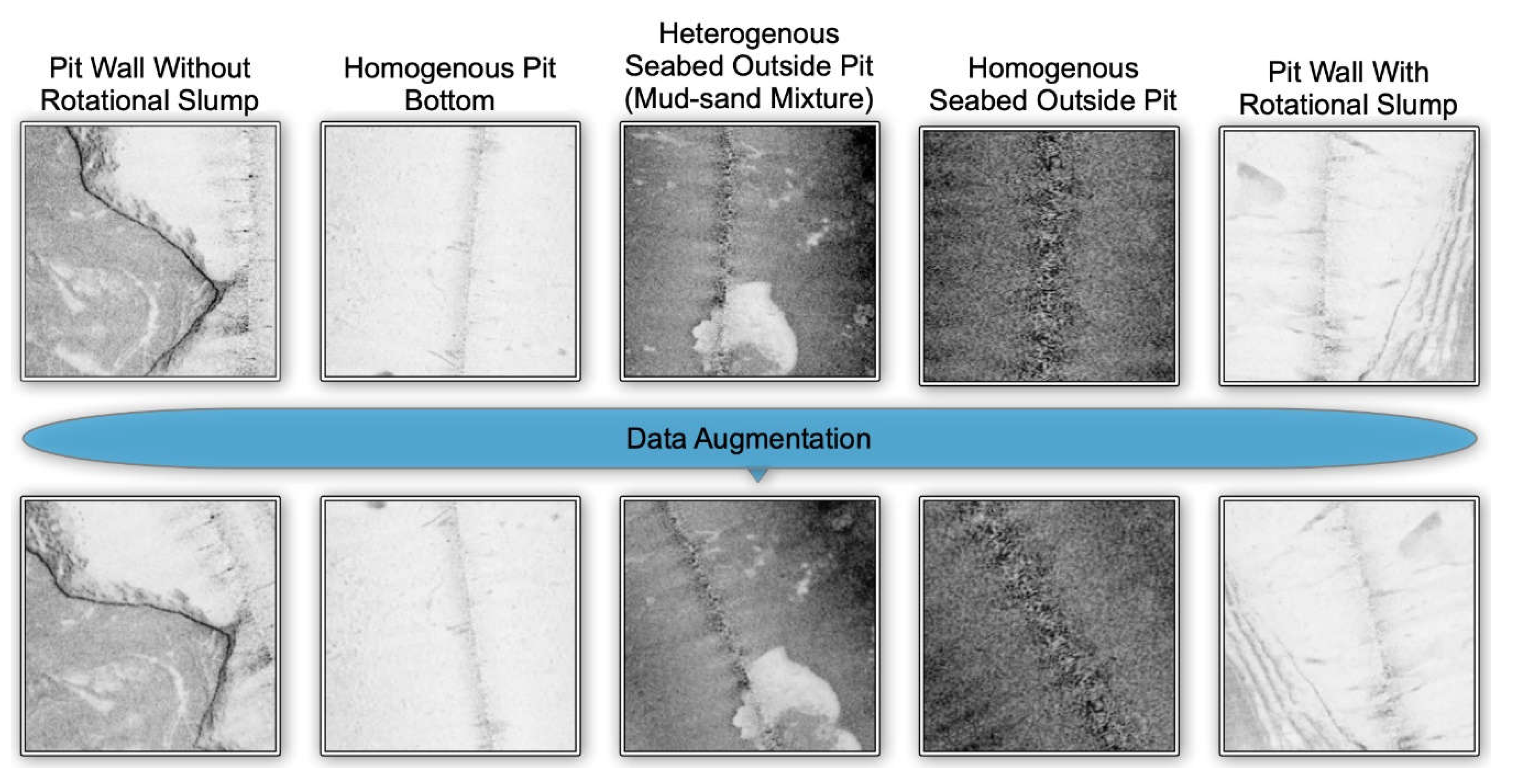
For the augment, the model transformed the images differently each time they are passed through the augmentation pipeline during training. This means each epoch can see slightly different versions of the same image, which helps the model generalize better from the training data by preventing it from memorizing exact details. These augmentation techniques were applied exclusively to the training set, ensuring that the model learns from a more diverse set of examples without altering the test sets. Examples of augmented images are shown in Figure .
Figure 4.
Examples of original and augmented images in five classes. The top row shows the original images, and the bottom row shows randomly augmented images. A total of 5 classes of environments were defined: pit wall with rotational slump, pit wall without rotational slump, heterogenous pit bottom (sand-mud mixture), homogenous pit bottom, as well as homogenous seabed outside pit.
After random augmentations, image samples were randomly shuffled to further enhance model robustness by preventing the model from learning unintended patterns from the order of the samples. Finally, images were divided into multiple batches according to the hyperparameter batch size.
2.2. Effective Geomorphology Classification Model
Although data augmentations are beneficial to increase the data varieties, our SPDP dataset still presents unique challenges to the design of the classification model due to its relatively small size and the unique and intricate features. These features are often subtle yet critical for accurate classification, requiring a model that can learn effectively from limited data without overfitting. Additionally, the model’s training efficiency and scalability are also valuable. Good training efficiency allows faster model training and inference and even achieve real-time inference when conducting the image collection at the same time. Good scalability allows customized model design for various sizes of available data, which is crucial for small and unique data like ours. Therefore, we introduce an Effective Geomorphology Classification model (EGC), which aims to balance the model performance and efficiency.
In this section, we first introduce the architecture of our EGC model. Then we introduce two main modules of EGC in detail: Feature Extractor and Classifier.
2.2.1. Model Architecture
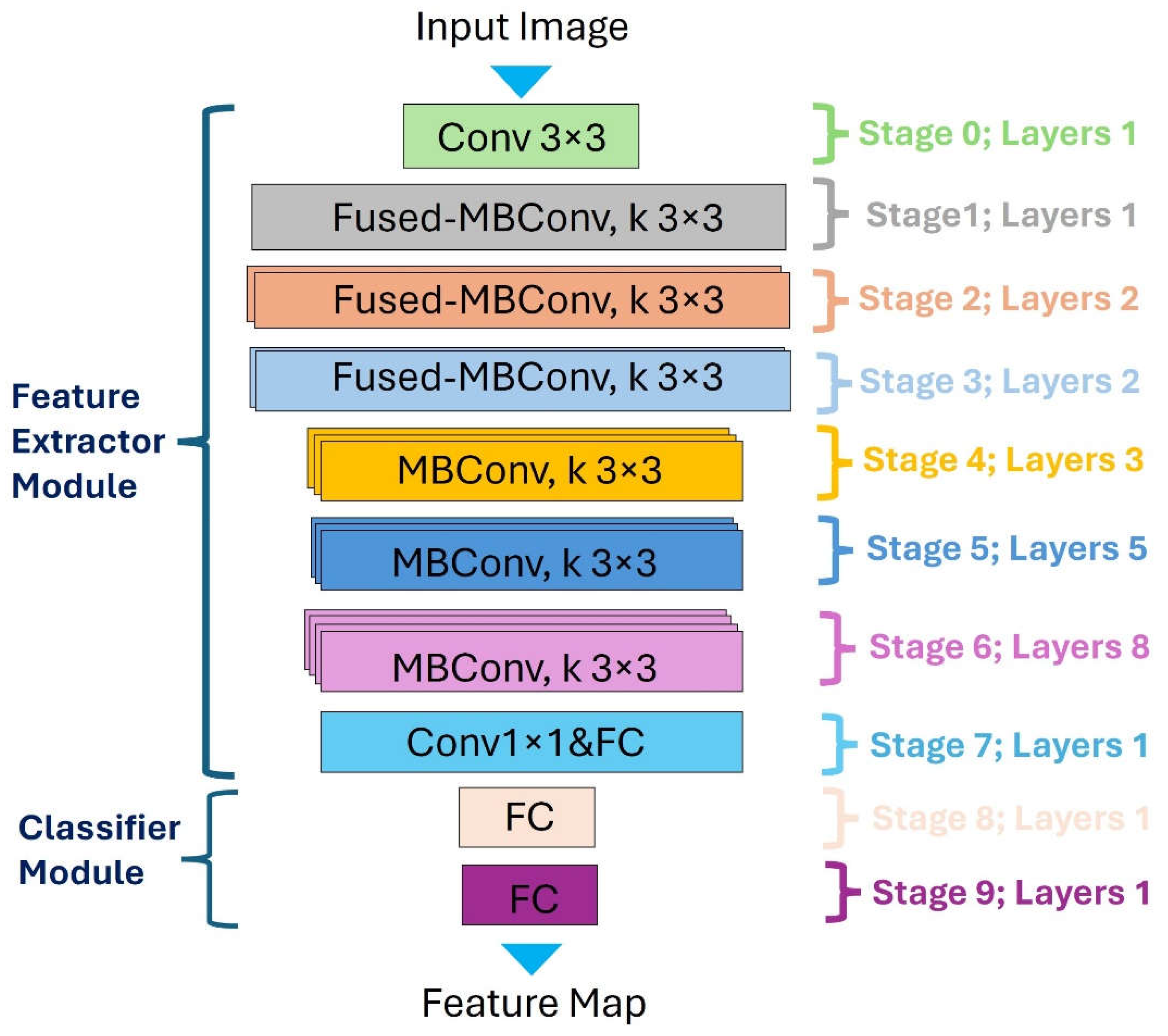
To balance the model performance and computational efficiency, we introduce an EGC model based on EfficientNet [37]. EfficientNet has shown good performance on image classification tasks with great tradeoff between accuracy and training and inference efficiency, which is achieved by its innovative scaling approach. EGC mainly has two modules: the feature extractor that adopts EfficientNet-B0 as the backbone to extract various levels of grains of geomorphology features, and the classifier that consists of two fully connected (FC) layers to perform predictions on five classes. The architecture of EGC is shown in Figure .
As shown in Figure , EGC was divided into 10 stages and all the layers in each stage have the same architecture. Stage 0-7 are the components of the feature extractor module and stage 8-9 are layers of the classifier module.
Figure 5.
Model architecture of EGC.
2.2.2. Feature Extractor Module
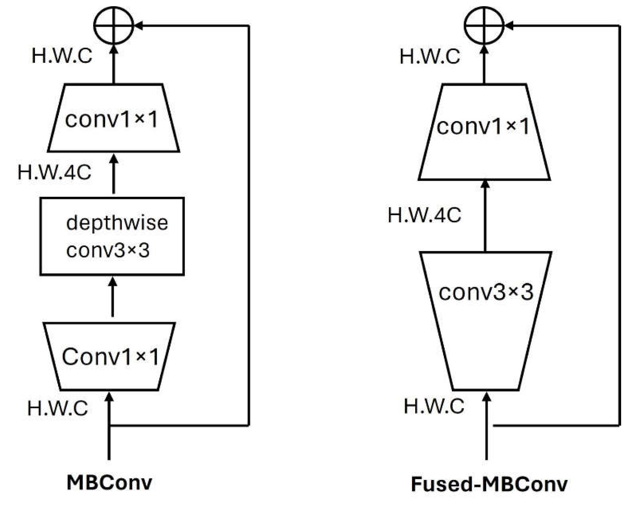
The foundation of our EGC is the feature extractor module, which meticulously processes the input sidescan sonar images to distill meaningful patterns. This module is designed to handle the nuances of underwater imagery with a good balance between model performance and model size. Two major convolution blocks were utilized in the feature extractor module: MBConv and Fused-MBConv, as shown in Figure . MBCov is the main convolution block in MobileNet [38], which consists of two convolution layers with kernel size of 1x1 and a depthwise block. Fused-MBConv is a variant of MBConv to achieve better training speed by replacing the depthwise conv3x3 and expansion conv1x1 in MBConv with a conv3x3.
Figure 6.
Structures of MBConv and Fused-MBConv blocks. .
As shown in Figure , the feature extractor module begins with a standard convolutional layer (Conv3x3) that is equipped with 32 filters of size 3x3 and has 32 channels. This serves as the initial feature extractor with the processed input images. The subsequent stages, 1 through 3, implement Fused-MBConv blocks. Fused-MBConv fuses the depthwise and pointwise convolutions into one layer for efficiency. They employ 3x3 kernels and exhibit an increasing complexity in terms of the number of channels, starting at 16 and progressing to 48. Each stage incrementally captures more complex features while managing computational efficiency. Stages 4 to 6 integrate MBConv blocks with 3x3 kernels. The number of channels in these layers progressively increases from 96 to 192, allowing the network to construct a highly detailed feature representation from the input data. Finally, a regular conv1x1 and fully connected layer generates the output with a vector of 1280 dimensions.
2.2.3. Classifier Module
The classifier module contains two fully connected layers where the output of the last layer is a vector of 5 dimensions, which corresponds to the number of classes in the geomorphology classification task.
Throughout the model, the number of layers within each stage varies, signifying the network's complexity and depth at different levels of abstraction. This hierarchical structuring enables the model to effectively learn both low and high-level features.
3. Results
3.1. Experimental Settings
In our experiments, we standardized the input image size to 224x224 pixels. Batch size is set to 8. Total training epochs are 400. We used Adam [39] as the optimizer, where a cosine decaying learning rate scheduler is applied with initial learning rate 0.001 and exponential decay rates are 0.9 and 0.999, respectively.
To evaluate the performance of our model, we utilized the top-1 accuracy metric. This metric is a direct measure of the model’s ability to correctly classify the primary sediment type from an image, providing a clear and interpretable assessment of the classification performance.
To evaluate the classification performance of our EGC model, we selected a range of CNN architectures as the backbones and connected them with the classifier module, each with varying complexities and characteristics. The specifications of baselines are shown in Table 2.
- LeNet [40]: One of the earliest convolutional networks, LeNet is renowned for its simplicity and effectiveness in image classification tasks.
- VGG16 [36]: A deep CNN renowned for its simplicity and depth, which has shown exceptional performance on various image recognition tasks.
- MobileNet [38] (Small and Large variants): MobileNet architectures are designed for mobile and edge devices, emphasizing efficiency. The ‘Small’ variant represents a more compact version, while the ‘Large’ variant is a scaled-up version with a higher capacity for feature extraction.
As shown in Table 2, our EGC has a middle size among baselines and middle number of FLOPs. The design of EGC is to balance the training efficiency and the model performance. Therefore, to fully evaluate the effectiveness of EGC on our small dataset, we need to further measure its prediction performance in the following sections.
3.2. Experimental Results
In this section, we present major findings of performance of our EGC model and ablation studies on some key components. All experimental results presented are averaged from 5 independent experiments.
3.2.1. Model Performance
Typically, training CNNs from scratch where all the parameters of the model are trainable on small datasets is difficult, because CNNs usually have a vast number of parameters that require substantial amounts of data to learn effectively without overfitting. When data are scarce, the model may not encounter enough variation to generalize well, leading it to memorize the limited training examples rather than learning the underlying patterns.
In this section, to evaluate the classification performance of our EGC model against baselines, we train each baseline model from scratch. Accuracy and convergence speed are shown in Table 3 and training curves are given in Figure .
Figure 7.
Performance of our EGC model against multiple baselines.
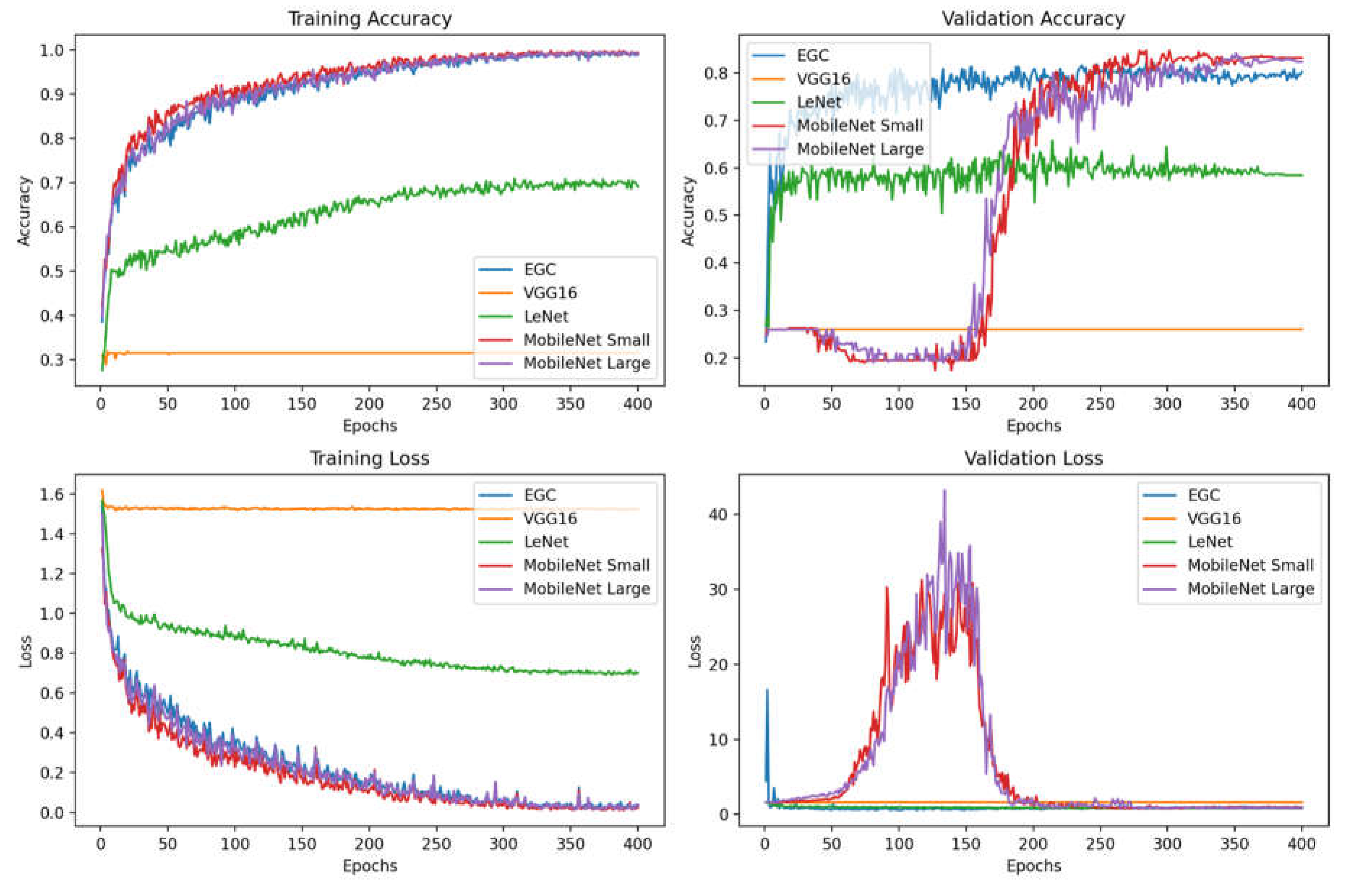
As shown in Figure , from the training accuracy and training loss curves, EGC along with MobileNet Small and MobileNet Large converge fast and reaches the performance plateau with more than 0.95 accuracy at about epoch 200, while LeNet and VGG16 converge to local minimum. It indicates that LeNet and VGG16 are underfitting and not able to effectively extract the key features from our sidescan sonar images.
As shown in Table 3, EGC has a significantly fast converge speed and good generalization ability which achieves a stable validation accuracy at 0.80 after only 96-epoch training. Although MobileNet Small and MobileNet Large have a slightly higher accuracy than EGC after 300-epoch training, they are much less robust than EGC with high fluctuations between epochs, shown in Figure . Moreover, MobileNet variants need about 150-epoch warmup to improve the validation accuracy, which shows significantly low training efficiency.
3.2.2. Transfer Learning Versus Training from Scratch
The decision to train a CNN from scratch or to employ transfer learning of the model pretrained from large dataset is critical to the success of the model training, especially when faced with a small dataset. In this section, we evaluate the performance of two variants of our EGC model: EGC, the one trained from scratch, and EGC (Pretrained), the one leveraging transfer learning. Specifically, the feature extractor module of EGC (Pretrained) is pretrained on ImageNet that is a vast and diverse image dataset, and the weights of feature extractor are fixed, which leaves only the classifier to be updated on our SPDP dataset.
It is worth noting that we also apply transfer learning to other baselines. However, only VGG16 (Pretrained) shows good performance and shows some interesting findings. Therefore, we add VGG16 and VGG16 (Pretrained) into the comparison. The results are shown in Figure .
Figure 8.
Performance comparison between EGC, EGC(Pretrained), VGG16, and VGG16(Pretrained).
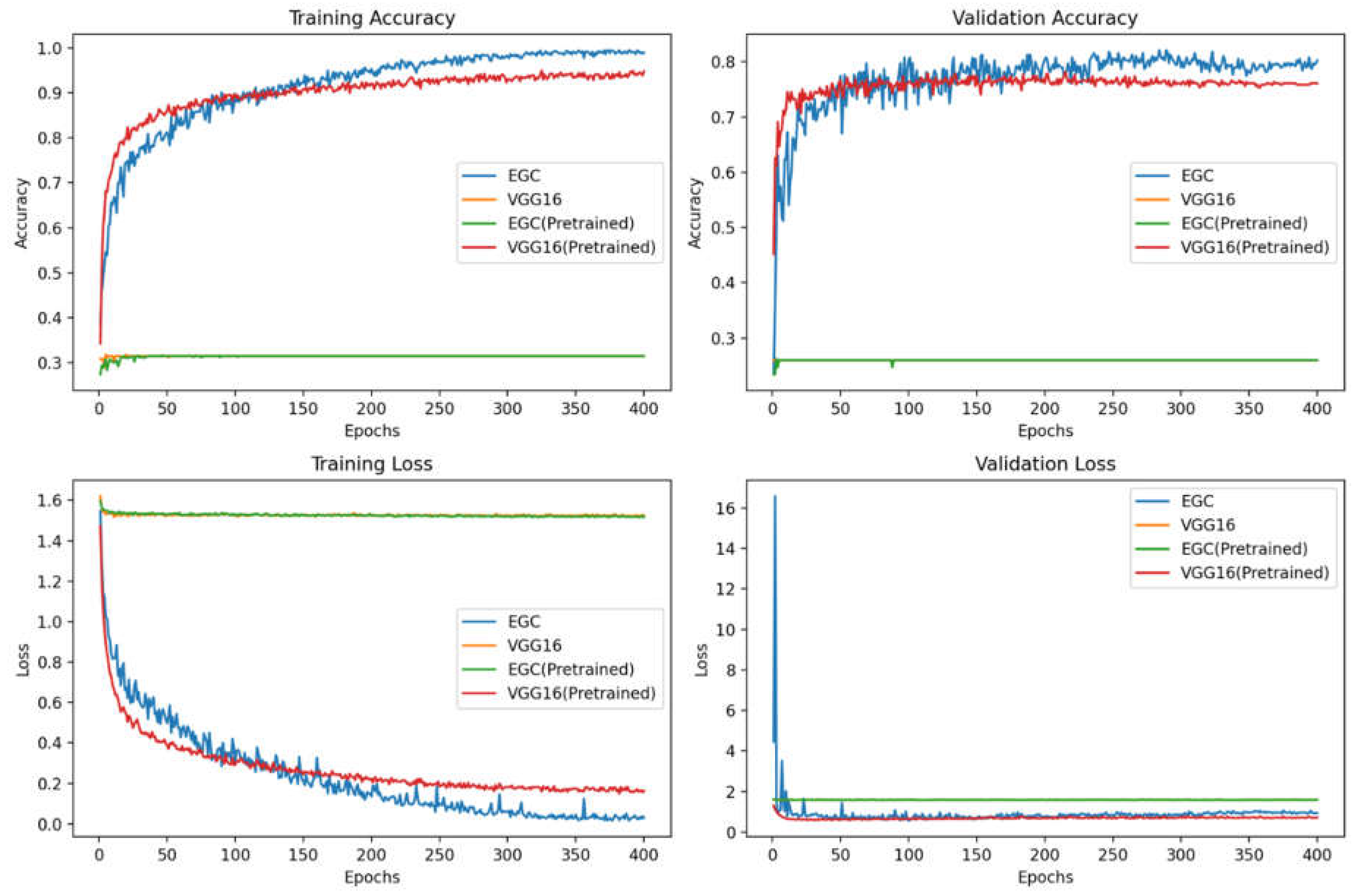
The EGC model, trained from scratch, demonstrates exceptional validation accuracy, indicating that its architecture is well-suited for the nuances of the dataset at hand. Its superior performance suggests that even without the benefits of transfer learning, the model is capable of learning robust and discriminative features specific to geomorphology classification.
Both VGG16 and EGC (Pretrained) exhibit signs of underfitting, as seen from their lower training accuracies. In the case of VGG16, this could be attributed to its depth and the large number of parameters, which may be difficult to train effectively without a sufficiently large dataset. For the pretrained EGC, underfitting could be due to the significant domain shift between natural images in ImageNet and the sonar imagery in our dataset. The model may struggle to adjust these features to the new task during fine-tuning, leading to poor performance in both training and validation phases.
Complex models like VGG16, known for their performance on large and diverse datasets, may not always be the optimal choice for smaller, domain-specific datasets. For these models, transfer learning is beneficial for reduced number of trainable parameters. Instead, more specialized architectures like our EGC can capture the essential features effectively without transfer learning.
3.2.3. Ablation Study on Image Processing
In this ablation study, we investigate the impact of data preprocessing on the performance of our EGC model. By comparing the EGC with and without these preprocessing steps, we aim to understand their contribution to the model's learning efficacy. The results are shown in Figure .
Figure 9.
Performance comparison between EGC, EGC (W/O Preprocessing).
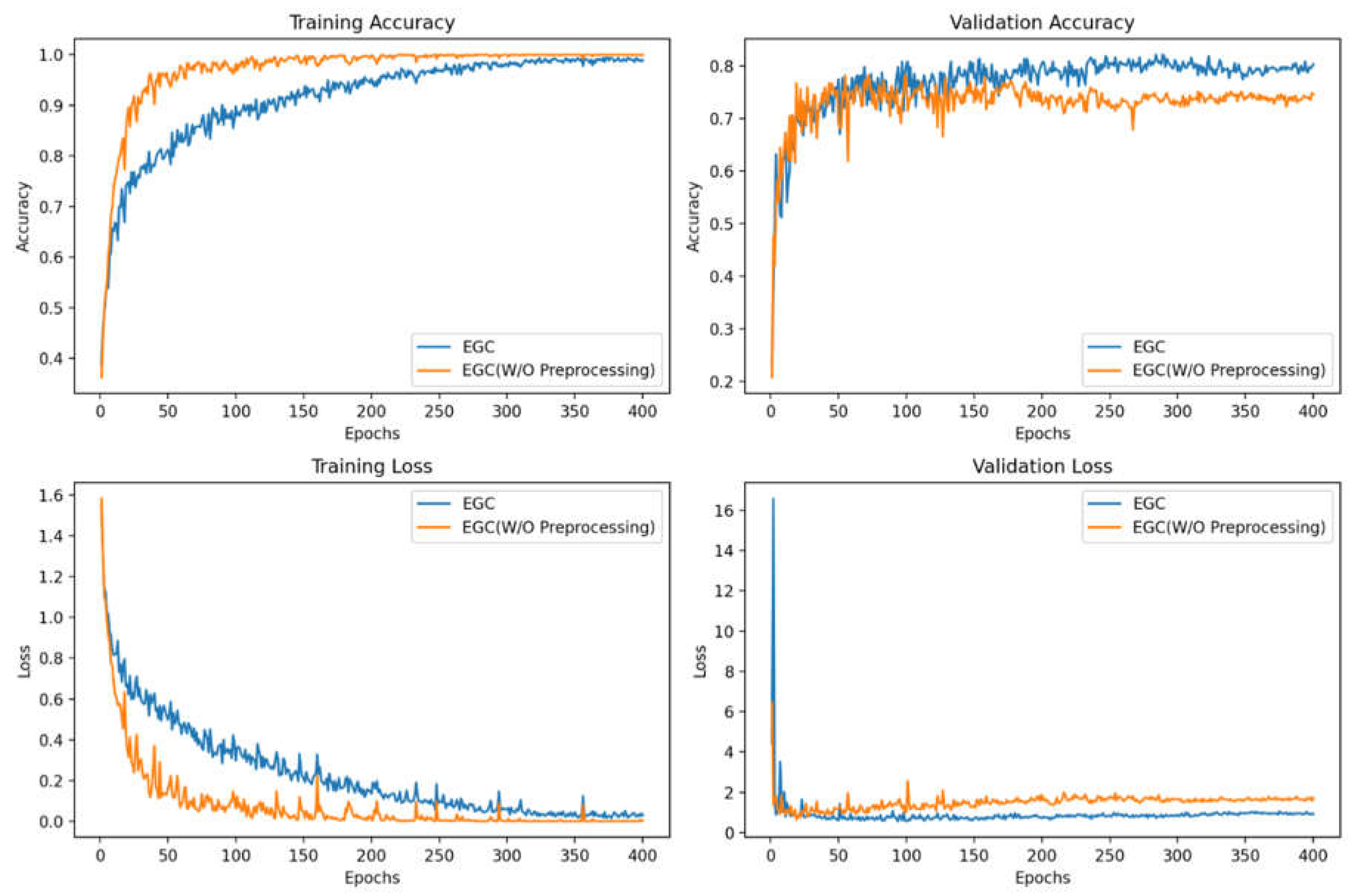
EGC is more resistant to overfitting and shows better generalization ability. Although EGC (W/O Preprocessing) initially exhibits a more rapid convergence during the early epochs of training, it begins to overfit after approximately 50 epochs, as evidenced by the divergence of training and validation loss. Moreover, EGC model, incorporating preprocessing steps, maintains a steadier convergence and achieves a higher validation accuracy by a large margin of 0.1. Overall, EGC shows better resistant to the overfitting and better generalization ability benefited from data processing.
4. Implementation and Limitation
In response to sea level rise and land subsidence, dredging is a global human activity to restore coastal environments and battle with land loss. It is anticipated that more dredge pits will be formed in the future decades. Detecting pit walls and calculating the distance from pit walls to oil and gas pipelines and platforms are critical to the safety of marine resource management. Data generated by EGC can help decision makers to better evaluate the setback buffer distance from pit walls to oil and gas pipelines and platforms which is about 1000 ft. Moreover, submarine landslides are a type of geohazard widely found in marine environments. Our EGC model can be adapted and easily applied to the detection of the walls of gullies and lobes formed in the areas of submarine landslides which can be triggered by hurricane waves, earthquakes as well as tsunamis.
Several machine learning studies related to dredging activities have been reported in recent years, which includes identifying sediment types and sand mining ([41,42]). However, utilizing machine learning methods to identify the geomorphic features like dredge pit walls is still very limited. In September 2022, [19] observed large mudslides on the west side of the Sandy Point dredge pit (Figure 1). This was the first time that mudslides occurred in dredge pits of muddy environments. This phenomenon has great implication to the safety of ambient gas and oil pipelines and platforms, as well as the communication cables. Therefore, sand and energy management and dredging related hazards require better monitoring tools.
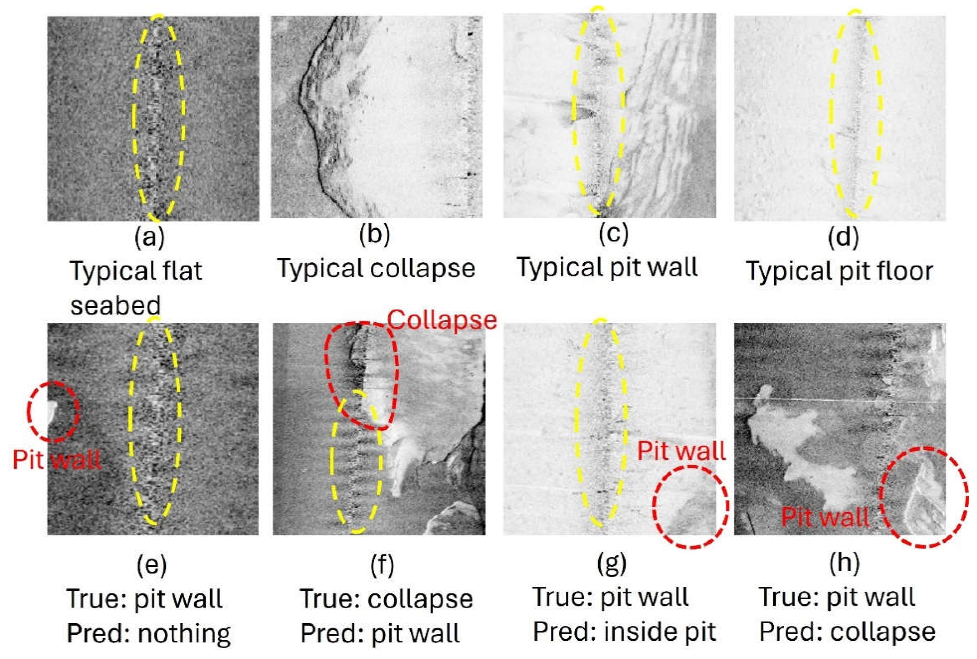
Compared with bathymetry and core, sidescan sonar data are easier to collect and process. In recent years, a large amount of SSS data has been collected in coastal marine environments. Therefore, the combination of SSS data and machine learning methods is a promising method to monitor the geomorphic evolution of dredge pits and secondary hazard along with the dredging activities. In this study, EGC shows a good balance between model performance and training efficiency. Furthermore, it can learn effectively from small data (Figure ). This indicates EGC has a promising future in dredging pit environments. Except the Sandy Point dredge pit, this EGC model could also be used in other dredge pits on the inner Louisiana continental shelf. EGC model has limitations in identifying the geomorphic features in the dredge pit environment (see Figure ). This could be a result of small dataset and the complexity of geomorphic features. For example, Figure e shows a wrong prediction which is likely because the pit wall fraction is too small and is quite different from the typical pit wall. Figure g and Figure h have similar problems. Besides, Figure f yielded wrong prediction because data noise makes the feature of collapse incomplete and unpredictable. Therefore, creating bigger SSS images dataset and more training could make the EGC model more accurate. Besides, a model specialized in identifying geomorphic features could be developed based on the EGC model.
Figure 10.
(a) ~ (d) are examples of typical features. (e) ~ (h) are examples for the wrong predictions. Red dashed circles highlight the target features. The yellow dashed circles highlight the noise produced in the nadir of SSS during the data collection.
Figure 10.
(a) ~ (d) are examples of typical features. (e) ~ (h) are examples for the wrong predictions. Red dashed circles highlight the target features. The yellow dashed circles highlight the noise produced in the nadir of SSS during the data collection.
5. Conclusions
Using machine learning model to identify the geomorphic features from the high resolution SSS images is discussed in this paper. The specific conclusions are as follows:
1. We introduced the EGC model to identify the geomorphic feature in marine dredge pit environment. The EGC model has the best training accuracy and validation accuracy among all other machine learning models (LeNet, VGG16, MobileNet Small and Large), the best training accuracy (among all models) is 96%, and the best validation accuracy (among all models) is 80%. Besides, EGC shows a better balance between model performance and training efficiency. Compared to other models, EGC model train from scratch has superior validation accuracy without transfer learning. The EGC model with preprocessing is more resistant to overfitting and shows better generalization ability.
2. Dredging induced mudslides is a threat to the ambient energy and communication infrastructures in the inner Louisiana continental shelf. The EGC model could be used to monitor the mudslides in dredge pits. Compared to bathymetry data, SSS images are easy to collect and process. The combination of SSS images and machine learning model (e.g. EGC) could be a promising tool for monitoring geomorphic evolution and mudslides under dredge pits environment. Besides, the EGC model introduced in this paper and the SSS images dataset are also valuable to other machine learning researchers.
Author Contributions
Conceptualization,W.Z.; formal analysis, W.Z., X.C., K.X.; funding acquisition, K.X.; methodology, W.Z., X.C.; software, W.Z., X.C.; visualization, W.Z., X.C.; writing – original draft, W.Z., X.C.; write – review & editing, K.X., X.Z., J.C., J.Y., T.Z.; All authors have read and agreed with the published version of the manuscript.
Funding
This paper was also funded by the Bureau of Ocean Energy Management Agreement Number M14AC00023, and Barton Rogers, Christopher DuFore, and Michael Miner served as the project officers of the Bureau of Ocean Energy Management. This study was partly funded by U.S. Coastal Research Program (W912HZ2020013) as well as National Science Foundation RAPID program (2203111).
Institution Review Board Statement
Not applicable.
Informed Consent Statement
Not applicable.
Data Availability Statement
Will publish the data after acceptance.
Conflicts of Interest
The authors have no conflicts of interest.
References
- Penland, S. , & Suter, J. R. (1988). Barrier island erosion and protection in Louisiana: A coastal geomorphological perspective.
- Penland, S. , & Ramsey, K. E. (1990). Relative sea-level rise in Louisiana and the Gulf of Mexico: 1908-1988. Journal of Coastal Research, 323-342.
- Stone, G. W. , & McBride, R. A. (1998). Louisiana barrier islands and their importance in wetland protection: forecasting shoreline change and subsequent response of wave climate. Journal of Coastal Research, 900-915.
- Miner, M. D. , Kulp, M. A., FitzGerald, D. M., Flocks, J. G., & Weathers, H. D. (2009). Delta lobe degradation and hurricane impacts governing large-scale coastal behavior, South-central Louisiana, USA. Geo-Marine Letters, 29, 441-453. [CrossRef]
- Maloney, J. M., Bentley, S. J., Xu, K., Obelcz, J., Georgiou, I. Y., & Miner, M. D. (2018). Mississippi River subaqueous delta is entering a stage of retrogradation. Marine Geology, 400, 12-23. [CrossRef]
- Van Heerden, I. L. , & DeRouen Jr, K. (1997). Implementing a barrier island and barrier shoreline restoration program: the state of Louisiana's perspective. Journal of Coastal Research, 679-685.
- Nairn, R. , Johnson, J. A., Hardin, D., & Michel, J. (2004). A biological and physical monitoring program to evaluate long-term impacts from sand dredging operations in the United States outer continental shelf. Journal of Coastal Research, 20(1), 126-137. [CrossRef]
- Kulp, M., Penland, S., Williams, S. J., Jenkins, C., Flocks, J., & Kindinger, J. (2005). Geologic framework, evolution, and sediment resources for restoration of the Louisiana coastal zone. Journal of coastal research, 56-71.
- Brunn, P., Gayes, P. T., Schwab, W. C., & Eiser, W. C. (2005). Dredging and offshore transport of materials. Journal of Coastal Research, 453-525.
- Thomsen, F. , McCully, S., Wood, D., Pace, F., & White, P. (2009). A generic investigation into noise profiles of marine dredging in relation to the acoustic sensitivity of the marine fauna in UK waters with particular emphasis on aggregate dredging: phase 1 scoping and review of key issues. Cefas MEPF Ref No. Fisheries & Aquaculture Science, Suffolk, 61.
- CEDA (2011) CEDA position paper: underwater sound in relation to dredging. Terra et Aqua 125:23–28.
- Tillin, H. M., Houghton, A. J., Saunders, J. E., & Hull, S. C. (2011). Direct and indirect impacts of marine aggregate dredging. Marine ALSF Science Monograph Series, 1.
- [WODA] World Organization of Dredging Associations. 2013. Technical guidance on underwater sound in relation to dredging. Delft (NL). 8 p.
- Todd, V. L. , Todd, I. B., Gardiner, J. C., Morrin, E. C., MacPherson, N. A., DiMarzio, N. A., & Thomsen, F. (2015). A review of impacts of marine dredging activities on marine mammals. ICES Journal of Marine Science, 72(2), 328-340. [CrossRef]
- CEC, & CECI. (2017). NRDA Caminada Headland Beach and Dune Restoration, Increment II (BA-143) Completion Report.
- Stone, G. W. , Condrey, R. E., Fleeger, J. W., Khalil, S. M., Kobashi, D., Jose, F.,... & Reynal, F. (2009). Environmental investigation of long-term use of Ship Shoal sand resources for large scale beach and coastal restoration in Louisiana. US Dept. of the Interior, Minerals Management Service, Gulf of Mexico OCS Region, New Orleans, LA. OCS Study MMS, 24, 278.
- Rangel-Buitrago, N. G. , Anfuso, G., & Williams, A. T. (2015). Coastal erosion along the Caribbean coast of Colombia: Magnitudes, causes and management. Ocean & Coastal Management, 114, 129-144. [CrossRef]
- Xue, Z. , Wilson, C., Bentley, S. J., Xu, K., Liu, H., Li, C., & Miner, M. D. (2017, December). Quantifying Sediment Characteristics and Infilling Rate within a Ship Shoal Dredge Borrow Area, Offshore Louisiana. In AGU Fall Meeting Abstracts (Vol. 2017, pp. EP13B-1620).
- Zhang, W., Xu, K., Herke, C., Alawneh, O., Jafari, N., Maiti, K., ... & Xue, Z. G. (2023). Spatial and temporal variations of seabed sediment characteristics in the inner Louisiana shelf. Marine Geology, 463, 107115. [CrossRef]
- Obelcz, J. , Xu, K., Bentley, S. J., O'Connor, M., & Miner, M. D. (2018). Mud-capped dredge pits: An experiment of opportunity for characterizing cohesive sediment transport and slope stability in the northern Gulf of Mexico. Estuarine, Coastal and Shelf Science, 208, 161-169. [CrossRef]
- Wang, J. , Xu, K., Li, C., & Obelcz, J. B. (2018). Forces driving the morphological evolution of a mud-capped dredge pit, northern Gulf of Mexico. Water, 10(8), 1001. [CrossRef]
- Xu, K. , Corbett, D. R., Walsh, J. P., Young, D., Briggs, K. B., Cartwright, G. M.,... & Mitra, S. (2014). Seabed erodibility variations on the Louisiana continental shelf before and after the 2011 Mississippi River flood. Estuarine, Coastal and Shelf Science, 149, 283-293. [CrossRef]
- Byrnes, M. R., Hammer, R. M., Thibaut, T. D., & Snyder, D. B. (2004). Physical and biological effects of sand mining offshore Alabama, USA. Journal of Coastal Research, 20(1), 6-24. [CrossRef]
- Kennedy, A. B., Slatton, K. C., Starek, M., Kampa, K., & Cho, H. C. (2010). Hurricane response of nearshore borrow pits from airborne bathymetric lidar. Journal of waterway, port, coastal, and ocean engineering, 136(1), 46-58. [CrossRef]
- Denny, J. F. , Baldwin, W. E., Schwab, W. C., Gayes, P. T., Morton, R., & Driscoll, N. W. (2007). Morphology and textures of modern sediments on the inner shelf of South Carolina's Long Bay from Little River Inlet to Winyah Bay (No. 2005-1345). US Geological Survey.
- Freeman, A. M. , Roberts, H. H., & Banks, P. D. (2007). Hurricane impact analysis of a Louisiana shallow coastal bay bottom and its shallow subsurface geology.
- Reed, S., Petillot, Y., & Bell, J. (2003). An automatic approach to the detection and extraction of mine features in sidescan sonar. IEEE journal of oceanic engineering, 28(1), 90-105. [CrossRef]
- Celik, T., & Tjahjadi, T. (2011). A novel method for sidescan sonar image segmentation. IEEE Journal of Oceanic Engineering, 36(2), 186-194. [CrossRef]
- Barngrover, C. , Kastner, R., & Belongie, S. (2014). Semisynthetic versus real-world sonar training data for the classification of mine-like objects. IEEE Journal of Oceanic Engineering, 40(1), 48-56. [CrossRef]
- Chandrashekar, G. , Raaza, A., Rajendran, V., & Ravikumar, D. (2023). Side scan sonar image augmentation for sediment classification using deep learning-based transfer learning approach. Materials Today: Proceedings, 80, 3263-3273. [CrossRef]
- Song, Y. , Zhu, Y., Li, G., Feng, C., He, B., & Yan, T. (2017, September). Side scan sonar segmentation using deep convolutional neural network. In OCEANS 2017-Anchorage (pp. 1-4). IEEE.
- Huo, G., Wu, Z., & Li, J. (2020). Underwater object classification in sidescan sonar images using deep transfer learning and semisynthetic training data. IEEE access, 8, 47407-47418. [CrossRef]
- Blondel, P., & Sichi, O. G. (2009). Textural analyses of multibeam sonar imagery from Stanton Banks, Northern Ireland continental shelf. Applied Acoustics, 70(10), 1288-1297.
- Nayak, N. , Nara, M., Gambin, T., Wood, Z., & Clark, C. M. (2021). Machine learning techniques for AUV side-scan sonar data feature extraction as applied to intelligent search for underwater archaeological sites. In Field and Service Robotics: Results of the 12th International Conference (pp. 219-233). Springer Singapore.
- Shaisundaram, V. S. , Chandrasekaran, M., Sujith, S., Kumar, K. P., & Shanmugam, M. (2021). Design and analysis of novel biomass stove. Materials Today: Proceedings, 46, 4054-4058. [CrossRef]
- Simonyan, K. , & Zisserman, A. (2014). Very deep convolutional networks for large-scale image recognition. arXiv:1409.1556.
- Tan, M. , & Le, Q. (2019, May). Efficientnet: Rethinking model scaling for convolutional neural networks. In International conference on machine learning (pp. 6105-6114). PMLR.
- Sandler, M., Howard, A., Zhu, M., Zhmoginov, A., & Chen, L. C. (2018). Mobilenetv2: Inverted residuals and linear bottlenecks. In Proceedings of the IEEE conference on computer vision and pattern recognition (pp. 4510-4520).
- Kingma, D. P., & Ba, J. (2014). Adam: A method for stochastic optimization. arXiv preprint arXiv:1412.6980. arXiv:1412.6980.
- LeCun, Y. , Bottou, L., Bengio, Y., & Haffner, P. (1998). Gradient-based learning applied to document recognition. Proceedings of the IEEE, 86(11), 2278-2324. [CrossRef]
- Liu, H. , Xu, K., Li, B., Han, Y., & Li, G. (2019). Sediment identification using machine learning classifiers in a mixed-texture dredge pit of Louisiana shelf for coastal restoration. Water, 11(6), 1257. [CrossRef]
- Kumar, S. , Park, E., Tran, D. D., Wang, J., Loc Ho, H., Feng, L.,... & Switzer, A. D. (2024). A deep learning framework to map riverbed sand mining budgets in large tropical deltas. GIScience & Remote Sensing, 61(1), 2285178. [CrossRef]
Figure 1.
(a) Map of Mississippi bird foot delta. (b) Bathymetry map for Sandy Point dredge pit. Bathymetric data of (a) are downloaded from ETOPO1 (https://www.ngdc.noaa.gov/mgg/global/). Oil platform and pipeline data are from BOEM website (https://www.data.boem.gov/). Bathymetric data of Sandy Point dredge pit were collected in May 2022 by [19]. ‘SPDP’ is Sandy Point dredge pit.
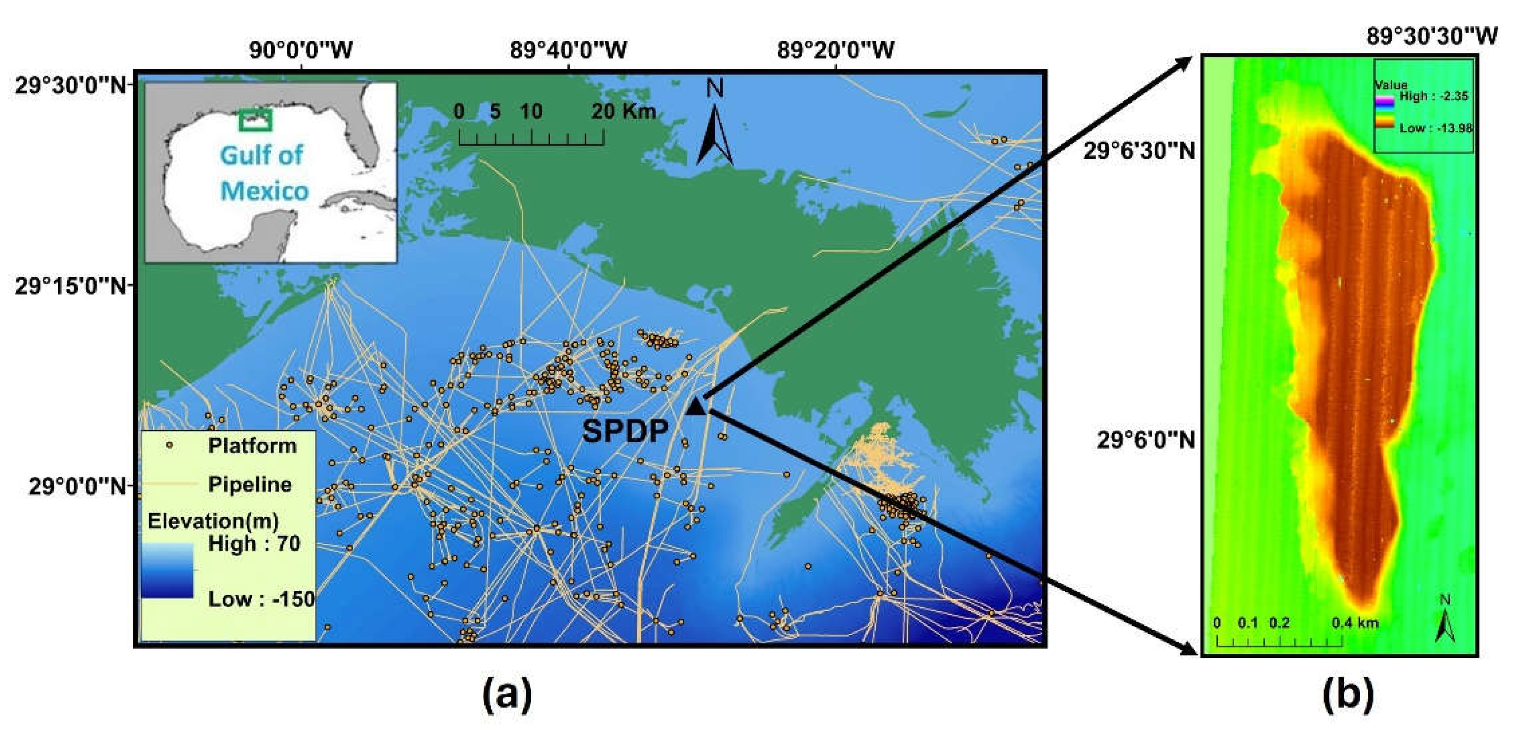
Figure 2.
(A) is the bathymetry data of Sandy Point dredge pit. (a)~(e) are five feature categories are highlighted by dashed circles. (B) is the whole picture of sidescan data. (C) is the examples of the data from each feature categories. The red squares are the examples’ location of the SSS images.
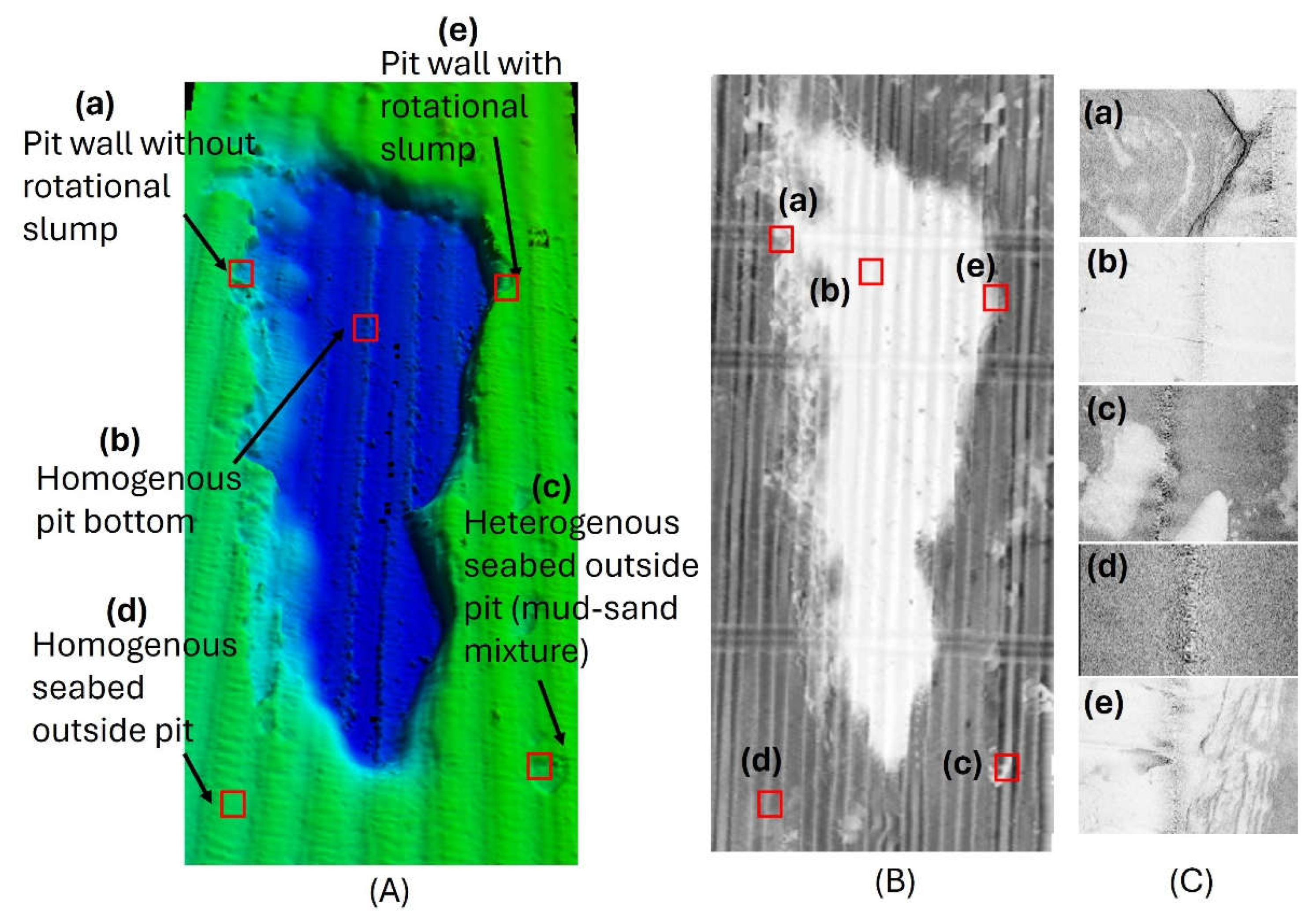
Figure 3.
Data preprocessing flow chart. Multiple data augmentation techniques were applied to increase the data diversity and prepared for the model training.
Figure 3.
Data preprocessing flow chart. Multiple data augmentation techniques were applied to increase the data diversity and prepared for the model training.
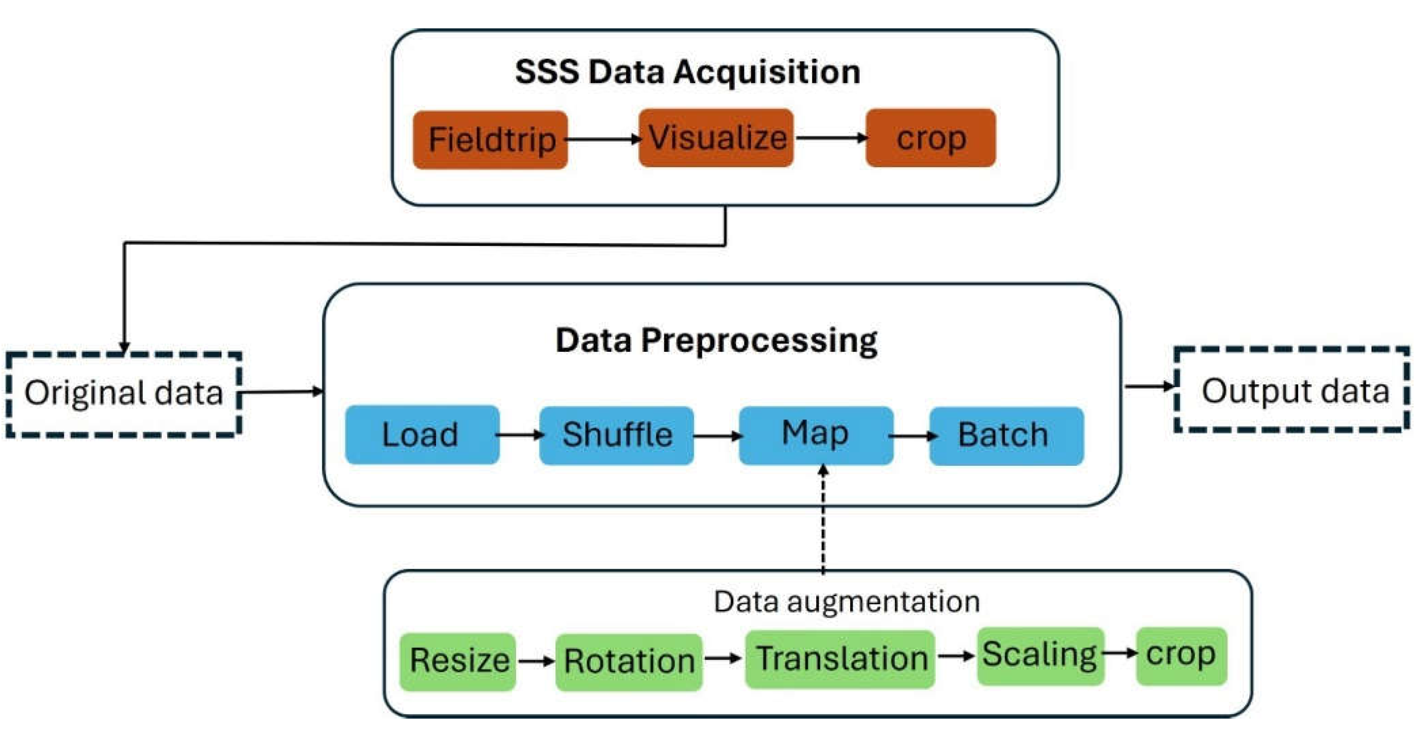

Table 1.
Specifications of SPDP dataset.
| Class | Training | Validation | Total |
|---|---|---|---|
| Pit wall without rotational slump | 28 | 7 | 36 |
| Homogenous pit bottom | 41 | 14 | 55 |
| Heterogenous seabed outside pit (mud-sand mixture) | 97 | 20 | 117 |
| Homogenous seabed outside pit | 78 | 15 | 93 |
| Pit wall with rotational slump | 64 | 21 | 84 |
Table 2.
The specifications of models. The number of parameters and float-point operations (FLOPs) has the unit of million.
Table 2.
The specifications of models. The number of parameters and float-point operations (FLOPs) has the unit of million.
| Model | #Parameter (M) | #FLOPs (M) |
|---|---|---|
| LeNet | 0.005 | 20.00 |
| VGG16 | 14.78 | 49.60 |
| MobileNet Small | 1.01 | 1.97 |
| MobileNet Large | 3.12 | 9.10 |
| EGC | 6.08 | 20.00 |
Table 3.
Classification performance and convergence speed of different models. Acc. denotes the best validation accuracy and Converge Epoch denotes the number of epochs required to achieve 0.80 validation accuracy. The best result is in bold.
Table 3.
Classification performance and convergence speed of different models. Acc. denotes the best validation accuracy and Converge Epoch denotes the number of epochs required to achieve 0.80 validation accuracy. The best result is in bold.
| Model | Acc. | Converge Epoch (Efficiency) |
|---|---|---|
| LeNet | 0.66 | / |
| VGG16 | 0.26 | / |
| MobileNet Small | 0.85 | 216 (2.25x) |
| MobileNet Large | 0.84 | 264 (2.75x) |
| EGC | 0.82 | 96 (1x) |
Disclaimer/Publisher’s Note: The statements, opinions and data contained in all publications are solely those of the individual author(s) and contributor(s) and not of MDPI and/or the editor(s). MDPI and/or the editor(s) disclaim responsibility for any injury to people or property resulting from any ideas, methods, instructions or products referred to in the content. |
© 2024 by the authors. Licensee MDPI, Basel, Switzerland. This article is an open access article distributed under the terms and conditions of the Creative Commons Attribution (CC BY) license (http://creativecommons.org/licenses/by/4.0/).
Copyright: This open access article is published under a Creative Commons CC BY 4.0 license, which permit the free download, distribution, and reuse, provided that the author and preprint are cited in any reuse.


