
Submitted:
14 August 2025
Posted:
18 August 2025
You are already at the latest version
Abstract
Maritime search-and-rescue (SAR) work typically involves scanning large sea areas looking for ships and related objects, where targets are sparse and appearance can be unknown. This labor- and capital-intensive task could be automated using reconnaissance drones and applying computer vision algorithms. In this work, the authors suggest the possibility of detecting man-made objects in marine backgrounds without prior knowledge of their appearance. The basis of detection is visual patterns (shapes), typical for such objects. Two algorithms were developed for this task: a deep learning fusion-based neural network consisting of a convolutional edge filter, an autoencoder, and a neural network (ANN), and a classical region-based detector built on Canny edges and geometric trimming. We curate a balanced dataset of 37,032 images (18,516 positive; 18,516 negative) derived from ships, platforms, and wind turbines and perform six-fold grouped cross-validation. The F1 score achieved by the artificial neural network-based method was no lower than 0.97, while 0.67 was scored by the region-based method. The result of the artificial neural network using a convolutional edge filter and a convolutional autoencoder was greater than those achieved by networks without such layers. The region-based method demonstrated an exceptional processing speed of 143 FPS. An algorithm involving both methods was proposed to be used for search and rescue operations using a drone. Results indicate that emphasizing shape primitives improves robustness to wave texture and reflections, limitations remain for very small targets. The experiment confirms the viability of using a shape-based method to detect objects characterized by distinct patterns in marine environments.
Keywords:
maritime
; ship
; detection
; drone
; computer vision
; fusion
; ANN
; region-based
; dataset
; search and rescue
1. Introduction
Instead of hindering scientific progress, a frequently overlooked positive characteristic of science is that it must inevitably fail to achieve the important task it is set out to do: discovery [1]. The human mind generates unique geometries in the design phase of development. It is therefore reasonable to believe that the search for man-made objects in a natural background can be enhanced by distinguishing these geometries from those generated by nature.
To date, maritime search and rescue (SAR) missions require satellites, planes, or helicopters. Satellite-based images cover significantly more ground. However, they lack resolution compared to aircraft-based images. The latter can cover tens of kilometers in radius. The ship-based detection radius is limited by the horizon occlusion caused by the roundness of the Earth. The proposed method should use aerial imagery, which offers greater coverage than the ship-based detection, but with a high enough resolution, so that the details are distinguishable. It has the potential to be used in conjunction with existing SAR methods, improving the accuracy of object detection. The goal is detection of any artificial object on open water (no shorelines), prioritizing robustness over class recognition.
Many ship detection methods rely on image segmentation or deep learning artificial neural networks (ANNs) trained on raw imagery. Image segmentation is sensitive to lighting and surface conditions (color, reflections), while ANNs rely on the size and content of the training dataset for detection performance [2]. Generalization is characteristic of ANNs. However, they are still struggling to recognize objects that were absent from the training dataset. When searching for debris, the object’s appearance, size, and number is not certain. Performance drops when targets are fragmentary or absent from training. Therefore, it is reasonable to train the network based on shapes, characteristic of man-made objects and their parts in the sea.
Furthermore, the sea exhibits varying colors, shapes and sizes of waves, lighting, reflections, and visibility conditions. Wave patterns generate high-contrast clutter and pseudo-edges. Such non-stationary backgrounds degrade detectors that rely mainly on intensity or texture. It is important to find man-made objects of uncertain appearance in this challenging background. Contemporary deep learning algorithms (Faster R-CNN, R-FCN, SSD, FPN, RetinaNet, and YOLO) mostly use training based on photos or video frames. In essence, RGB or grayscale images, containing objects, are used as input. The first layers of deep convolutional neural networks (CNN) respond to the distribution of spots, colors and textures [3]. The human brain, on the other hand, first responds to the peculiarity of shapes [4,5]. In this work, it is suggested to focus on the detection of shapes rather than attempting to recognize objects from all the visual data, including spots, textures and colors. The authors suggest using algorithms that are sensitive to the shapes contained in the image. In this work, a hybrid algorithm is proposed, which is expected to be capable of detecting man-made object debris in marine waters. It is composed of a region- and an ANN fusion-based methods. This might improve the differentiation between the natural and man-made geometries. Furthermore, the authors hypothesize that, in search of ships in seas, where objects are sparse, it is reasonable to search for any artificial object, instead of recognizing it.
The purpose of the method is to detect any artificial objects on the surface of water from aerial images, including various lighting and waving conditions. Both crewed and uncrewed aerial vehicles are suitable for image capture. The latter, however, could be more suitable for automated tasks, such as search due to reduced weight, cost, and risk of human error. The finished algorithm could be used to search for lost vessels, debris in SAR missions, as well as collision, contraband prevention and unfriendly marine drone detection [6]. We now outline detector families relevant to open-water imagery(satellite and aircraft/UAV) and the datasets used in practice. Given our scope (any artificial object on water, no shorelines) and the likelihood of partial/previously unseen targets, we prioritise approaches whose cues are robust to sea-state and illumination changes.
1.1. Related Work
To date, algorithms have been mostly developed to detect ships using satellite imagery [2,6,7]. However, this source suffers from cloud occlusion as well as lower resolution [9]. Some authors suggest detecting ships from other ships [10]. This greatly reduces the coverage area both in terms of the direct line of sight and the ability to move quickly. As for drone operations, Wang et al. reason that for specialized purposes, such as SAR, specialized datasets should be used [8], including applicable camera angles and objects. To get a general understanding of the state of the art in ship and debris detection, such topics should be covered: satellite-driven object detection, aircraft-driven object detection and datasets used for object detection experiments.
According to Li et al. [2], there are several main ship detection methods. The coastline matching method is based on knowledge of the precise position of the shore line. Objects in the sea are assumed to be ships. Regional homogeneity classification and methods based on statistical modelling work by dividing the image into segments and deciding which segment is a ship. Deep learning methods use data-based training to perform the detection, while methods based on normalized difference water index relies on multispectral camera imagery to detect which part of the sea reflects light differently than water. It is assumed that all of these methods are also suitable for other artificial marine object detection with some confidence. Let us analyze existing ship detection methods.
1.1.1. Satellite-Driven Floating Object Detection
While searching for ships in satellite imagery, one can be certain that they will always remain within a background of water. In essence the objects will not protrude the horizon. This is beneficial, because the background of the ship is more constant (it is always surrounded by water). Ships can be detected by removing repetitive background. As described by Li et al. [2]. Moreover, satellite imagery cannot capture high detail, which is relevant for feature extraction. Several methods can be used in such scenarios: Dong et al. divide the ship detection problem into separate tasks of detection and position determination [12]. Object detection methods can be divided into two categories: classic methods and deep learning. Classic methods include segmentation, such as clustering, threshold, region, edge, and watershed-based methods, and generally perform positioning less accurately [9]. Another group of classic algorithms is called primitive search and includes such methods as region analysis [10], Haar feature search [11,15] and the Hough transform [16]. as well as classic machine learning. They are considered less accurate than deep learning-based methods, such as R-RCC [12], SPP-net [13] Fast and Faster R-CNN [19] deep learning algorithms. Coverage and persistence are strong, but spatial detail and revisit constraints limit small-object detection; satellites often hint aircraft/UAV assets.
1.1.2. Aircraft-Driven Floating Object Detection
When using an aerial platform as a source of imagery, the captured object may protrude from the horizon or stay below, depending on the position of the object and the sensor height above the surface. The object may also be seen from various angles, distances, and lighting conditions. Moreover, it can be partially occluded by obstacles or the horizon [14,15]. The problem of how to detect objects with a background of the horizon as well as other objects is addressed by Hong et al. They have utilized and enhanced the YOLOv4 algorithm for higher performance and detection accuracy. The problem was partially solved by applying coastline feature segmentation to segment the sea and air. The interference targets on the shore can be separated, the number of bounding boxes can be reduced, and the detection time can be saved. This algorithm is also capable of detecting and tracking multiple objects simultaneously [21]. Cheng et al. have used a drone to detect ships in the sea using deep learning ANN-based YOLOv5-ODConvNeXt algorithm. The algorithm was optimized to achieve greater accuracy and faster processing than YOLO v5s, making it more suitable as an airborne platform [16]. Xiao-Sheng et al. suggest using drone swarms instead of a single drone. This would increase search area or resolution, as well as allow us to determine the position of a detected object more accurately by triangulation and redundancy. Some of the algorithms utilized for such tasks include Faster R-CNN, YOLOv5, CenterNet (Hourglass104, ResNet101, ResNet18), FairMOT R34, Tracktor++, Atom, DiMP18, PrDiMP18, PrDiMP50, DiMP50 [17,18]. For tracking, an unscented [19,20] or non-linear [21] Kalman filter can be used. Tracking improves detection accuracy, since temporally inconsistent detections can be eliminated.
The methods analyzed do not emphasize the importance of the characteristics such as shape or other visual pattern of the object. We therefore test whether explicit shape emphasis improves robustness in open-water scenes without shorelines.
1.2. Related Datasets
Only two datasets were found to contain drone-based marine object imagery. SeaDroneSim [22] was created as a benchmark and contains real and simulated images of a water rover BlueROV. The purpose of the training dataset was agricultural; however, the authors suggest using simulated data for SAR-related object detection. Another relevant dataset is SeaDroneSee [17], a drone-based aerial dataset consisting of more than 54,000 frames that contain instances of people in water and on board, as well as small boats. This dataset is aimed at helping train computer vision algorithms for SAR. All other datasets [27,28,29,30,31,32,33,34] containing found marine objects were collected or simulated as satellite images. They are aimed at detecting whole ships and other objects with few details. The dataset presented in this work contains relatively detailed ship fragments with no shoreline, which is argued to be effective in SAR missions involving lost or wrecked ships. The datasets which have been covered are listed in Table 1.
2. Materials and Methods
2.1. Dataset
After the analysis of the existing datasets, it was concluded that there is a need for a new dataset suitable for artificial object detection algorithm training. In order to satisfy this need, such a dataset was created and includes marine objects such as cargo ships, gas carriers, military ships, tankers, oil rigs, and windmills. It was assumed that the shape-based algorithm would be able to find all marine objects featuring similar geometries.
To test the algorithm capable of artificial object detection, a dataset containing the ground truth is required. In total, 3086 images of artificial marine objects were collected. This includes cargo ships (400 images), gas carriers (323 images), military ships (1243 images), tankers (105 images), oil rigs (538 images), and wind powerplants (377 images). The same number of images containing only the sea surface were obtained from open sources. Each image was resized to 256x128 pixels and divided in half in such a way that the dataset was doubled and each photo did not necessarily contain a whole maritime object, but only a cropped segment (in case of positive instances). After cropping, the augmentation of the dataset was applied using a blur filter and a gamma reduction. In the final dataset 18,516 images of maritime objects (Figure 1 (a)) and 18,516 images of sea (Figure 1 (b), (c)) were present in RGB, grayscale and edge formats. The dimensions of the final images were 128 pixels high and 128 pixels wide. According to Poolsawad et al., an equal class balance is desirable for training, while undersampling improves certain metrics associated with negative class predictions [31].
The background of the sea, especially the waves, might complicate the detection. Images of a calm and wavy sea were selected as the basis of the negative ground truth. The size of the waves in the image depends on the perspective, distance from the sensor to the surface, type, and size of the waves. A diverse selection of sea images was included in the dataset, including images taken from a long distance and containing an abundance of reflections (Figure 1 (c)).
The balanced dataset contained 37,032 images (18,516 positive; 18,516 negative). We used six-fold cross-validation with per-fold class balance. In each of six iterations, a different one-sixth of the data served as the validation set and the remaining five-sixths for training, so that each image was validated exactly once. We adopted k-fold to obtain more reliable averages across splits and to limit sensitivity to any single partition. Such a cross-validation method enables per-fold confusion matrices to be comparable.
2.2. Algorithm Description
Apart from the dataset, two algorithms have been implemented and tested in this work: a classic region-based detection method involving contour perimeter, area, and complexity calculation as well as a novel approach to an ANN-based detection involving contour emphasizing convolutional layer. They are explained in the next sections. The use of the two algorithms allows for a comparison of classic and modern methods. Furthermore, the region-based method is expected to complement the ANN-based approach in cases where the sea is calm, and the objects are small. In this way, the problem of small objects, which are hardly detectable by ANN, is addressed. Research is done concerning such object detection by ANN [32], but in this work for such application a classic detection algorithm is suggested. Furthermore, since it is hypothesized that it is reasonable to search for any artificial object, instead of recognizing it, an assumption is made, that the shoreline will be classified as an anomaly in the sea. Therefore, the proposed method is applicable only to images with a marine background and without a shoreline.
2.2.1. Region-Based Detection
The Canny edge detection algorithm can detect object boundaries in images. It is the basis of the region-based algorithm. Canny is one of the most advanced edge detection algorithms. Using this algorithm, contours of objects and waves are extracted [33]. It is robust against false boundaries and reacts to edge curves only once, which is relevant when the curves are wide. In an ideal case, an algorithm capable of extracting only man-made object contours would be used. The region-based method starts by extracting contours in the format of polygons using the Canny edge detector with the lower and the higher thresholds set to 250 and 300 respectively. These values were chosen based on the results of an iteration-based optimization method. The algorithm converts greyscale images to edges. Mean pixel value is then calculated from negative and positive dataset edge images. The assumption is that the mean value in the negative dataset has to be near 0, since our goal is to remove any background. At the same time, in the positive the edge values will also be decreasing. Therefore, in the ideal case there will be some threshold, using which there will be no background information left and only the object will be visible. Canny threshold values were increased iteratively until the point where the negative dataset mean pixel values started approaching 0, while positive values had not started decreasing significantly. The optimization algorithm increments the edge values by 50 starting from 50 as the lower threshold and 100 as the higher one. The mean values from the positive and negative dataset are provided in Table 2:
The region-based method then calculates the perimeters of the polygons from the detected edges. After this, polygonal curves are approximated, and areas of the polygons are calculated. Edges are then filtered by the size of their perimeter (≥500 px), line count (≥4) and area (≥ 20,000). The larger ones remain to become the result of the detection algorithm. Using these steps waves are discarded and ships - detected. No temporal smoothing is applied in this stage, tracking is reserved for future work. The algorithm workflow is depicted in Figure 2.
2.2.2. Fusion ANN-Based Detection
It is hypothesized that by extracting object contours before detection, accuracy can be improved. One of the ways to achieve this is image preprocessing using classic edge extraction and filtering methods in order to distinguish the shape and remove the noise, such as waves and sun reflections contained in the image. The following architecture is proposed: a convolutional edge detection filter, after which an autoencoder-like segment would distinguish dominant objects while reducing noise. This would then be fed to a CNN, all fused to be part of the ANN architecture, with the expectation of improved performance. Based on this hypothesis, an ANN architecture concept was developed, which included the fusion of several elements: a convolutional filter, an autoencoder, and a CNN (Figure 3).
The Sobel filter was included in a neural network by Sharifrazi et al. The inclusion of a Sobel filter in a CNN support vector machine algorithm improved the classification accuracy, sensitivity, and specificity compared to the one without the filter [34]. The autoencoder can be used for tasks where the input image is noisy [35]. In this work, we have included a convolutional autoencoder as a segment of the neural network algorithm (Figure 3).
First, the data enters the network through input neurons. There, the pixel values are rescaled, and a Sobel-like convolutional filter is applied to extract contours contained in the image by emphasizing gradients. This can be done using Canny edge detection, as in the case of the region-based method, but at a higher computational cost compared to Sobel or other convolutional filters, thus sacrificing real-time performance [36]. Another advantage of convolutional filter integration into a neural network architecture is the possibility of GPU computations. The shape and values of the convolutional filter are presented in Figure 4. There should be a separate filter for each channel. Meaning that an RGB image would be processed by three filters. An example of the convolutional edge input and output is provided in Figure 5. A grayscale image is depicted in Figure 5 (a), while convolutional filter output, using parameters from Figure 4, is depicted in Figure 5 (b).
Next, convolutional autoencoder-like layers are included for feature extraction. A classic autoencoder would require separate training [37], therefore it was not used. A classical autoencoder consists of an input, encoder, decoder, and output. The output of the encoder is a compressed representation of the input vector (Figure 6).
An autoencoder is trained on a dataset to transform the input vector to a state commanded by the support vector. In our case, the autoencoder is not a separate algorithm. It is fused with the convolutional filter and CNN; therefore, it is not trained separately. The input vector is supplied to the common network input during training.
In our work, the CNN is part of the ANN algorithm architecture. A conventional CNN was used, as described by Alzubaidi et al. [38]. The network was constructed by pooling several kernel convolution layers. These layers perform feature extraction and sub-discretization [42]. The main processing takes place in the kernel layers, in which convolutional and max pooling layers are arranged alternately. The output vector is processed by flattening and dense layers (Table 3). The max pooling layer decreases the feature map size. The convolutional feature map is associated with the previous layer and divided into regions according to the size of the pool. The last dense layers of the network estimate the classification probability values [36].
2.2.3. Hyperparameter Optimization
The hyperparameters of the CNN (filter count, layer count) as well as the activation function type were tuned for high performance.
First, the number of filters in the CNN core layers was treated. The number of filters also depends on number of the layer in the sequence. To describe the number of filters in a layer, such formula is used:
(4)
Where x is the number of filters in a layer, filterFactor is the multiplier coefficient, which is iterated from 1 to 8 in this optimization step, n is the number of the convolutional layer in the CNN sequence.
In the second step, the number of CNN convolutional layer pairs (convolution and maximum pooling layers) is iterated from 1 to 5 pairs.
In the third step, several activation functions (ReLU, Leaky ReLU, softmax, and sigmoid) were iterated. Each combination of the hyperparameters was matched, resulting in 160 different neural network configurations. Each network was tested on 6 dataset combinations, so 960 tests were made in total. Each network was trained for 3 epochs and compared. It was assumed that this is enough to judge the training tendency. The iteration cycle structure is depicted in Figure 7. The chosen network combination was trained for 30 epochs.
The final composition of the algorithm used in this work is presented in Table 3. The ANN input vector is 128 by 128 pixels of the encoded edge image in grayscale. The ANN output is a rectified linear unit (ReLU) function.
The algorithm was programmed using the Keras 2.13.1 library in Python 3.8. A dataset was loaded using a standard Keras loader. The custom neural network architecture was programmed using only standard TensorFlow modules. The confusion matrix metrics were output using the model predict function on the dataset images.
2.2.4. Evaluation
The task of the algorithm is the recognition of marine objects; therefore, the dataset was binary – positive images contain such objects, negative images – do not. This made the evaluation relatively straightforward, as only a true or false guess could have been made by the algorithm. The true positive (TP), false positive (FP), true negative (TN), and false negative (FN) guesses were counted to form a confusion matrix. From this, performance metrics (accuracy, precision, recall, and F-1 score) were calculated.
Recall is a property of the model to find relevant objects (least false negatives), while precision is the property to make only correct guesses (least false positives). These values change depending on the confidence level required for detection, typically inversely to each other. With high confidence, one might avoid many false positives; however, more objects will be missed, yielding a higher number of false negatives and vice versa. Accuracy is a measure of how correctly a model predicts the outcomes of the data it is trained on or tested against. It represents the proportion of correct predictions made by the model out of the total number of predictions. The F1 score represents both precision and recall as one metric. It is the harmonic mean of these measurements. The harmonic mean is used instead of the arithmetic mean to ensure that the F1 score is influenced more by the lower of the two values (precision or recall). This means that the F1 score will be high only if both precision and recall are high.
This study aimed to evaluate the suitability of region- and ANN fusion-based object recognition algorithms for man-made maritime object detection. For comparison, three other algorithms: simple CNN and MobileNet, were trained and tested on the dataset. Simple CNN is the same model as described in Section 2.2.3, but the edge detection and autoencoder-like layers are missing. This was done in order to quantify the performance gain using this combination. The proposed algorithms are also compared to the performance metrics and processing speed of MobileNet, a CNN optimized for performance at small network sizes and high speed [39].
After each convolution operation in an ANN a feature map is generated. On some maps from the first layers, important features may be highlighted and manually identified. Another way to identify the influential features is by using a saliency map. It provides insights into which parts of the input data (such as an image) are most influential in the prediction process. After the prediction is obtained, backpropagation is used to compute the gradients of the prediction result with respect to the input data. During back-propagation, the difference (loss) between a prediction and the ground truth in a binary classification task is calculated using the binary cross-entropy loss function. This loss function penalizes the model more when it makes confident incorrect predictions. The error is propagated backwards through the network to adjust the parameters (weights and biases) of the model. The gradients obtained from backpropagation are then used to create a saliency map. This map highlights regions of the input data that have the most significant impact on the model’s decision. Typically, brighter regions in the saliency map correspond to areas that strongly influence the model’s prediction. In this work, feature as well as saliency maps were extracted for performance analysis.
2.2.5. Algorithm Integration Concept
The area which is covered by the field of view of the camera is called the region of interest (ROI) (Figure 8). The view contained in ROI could be split into frames, which would then be processed by the algorithms described in this work to determine whether the frame contains recognizable (ship) patterns. The basis of the detection is an algorithm consisting of several steps depicted in Figure 9.
In the next stage, clusters are formed from the detected objects. This is done using the k-means method with n = 1 [40]. This allows one to detect at most one object in an image. It is suggested to use separate clustering algorithms for each detector, since the two algorithms work differently. Therefore, the results they produce may also differ.
The cluster coordinates are then sent to a Kalman filter, which tracks the target even in the presence of wave noise and other sources of error. It enables improvement in object tracking [24] if it is desired to keep the object in sight, and detection accuracy if a detection is made in several consecutive frames. Unfortunately, this method is incapable of distinguishing one target if multiple clusters are present. The diagram of the algorithm is presented in Figure 9.
3. Results
3.1. Region-Based Method Detection
The confusion matrix of the region-based method represents a considerable number of false positives and negatives. On average, 1292 false negative and 348 false positive detections were made out of 3086 instances each (Table 4). Possibly, the algorithm is less capable in wave and reflection rich environments.
The accuracy of the region-based method does not fall below 0.72. Furthermore, the lowest precision values exceed 0.82. The reason for this is a low number of FPs (Table 4). It can be assumed that the region-based method is sensitive to image noise and performs adequately only when the water surface contains few waves or sun reflections. Concerning the recall metric, it was observed to only reach a value of 0.57. This is due to a large number of false negatives. The F1 score exceeds 0.68 (Table 5). This value is influenced by the high TP to FN ratio. It is reasonable to use better denoising algorithms when the region-based method is utilized.
3.2. ANN-Based Detection
After training, the accuracy and F1 scores achieved were not less than 0.97, while recall and precision were not less than 0.99. The network was trained for 33 epochs and did not show signs of overfitting (Figure 10).
The results presented a low ratio of false negatives (FN) to true negatives (TN) and an even lower ratio of false positives (FP) to true positives (TP) (Table 6). From this, accuracy, precision, recall, and F1 score metrics can be calculated (Table 7). The low FP and FN values confirm that the ANN detects ship geometries correctly and that the wavy background is ignored. After a manual inspection, it was concluded that some of the false negative instances were too small to be detected. Possibly because of the lack of detail.
3.3. Algorithm Comparison
To see how the newly developed algorithms compare to the existing ones, simple CNN and MobileNet architectures were trained and tested on the dataset. This was done on a machine featuring a 13th generation Intel® Core™ i9-13900KF CPU, GeForce RTX™ 4090 SUPRIM X 24G GPU, Windows 11 Pro 23H2, Python 3.11.5. and Keras 2.15.0. Overall, the fusion-based ANN performed very well and came out first in most metrics. It was outperformed by MobileNet in recall, which demonstrated marginally lower accuracy and F1 scores. The frame rate of MobileNet was the lowest of all. The region-based detection algorithm performed the worst in all metrics. However, it offers the highest speed, nearly four times that of the fusion-based ANN. The simple CNN performed worse than the fusion-based ANN or MobileNet, but the results are still comparable. Its speed was only marginally lower than the fusion-based ANN (Table 8).
4. Discussion
In this work, two algorithms were developed and tested on a balanced dataset, which was created for this purpose, an algorithm implementation concept was presented. The augmented dataset contains 18,516 images of several types of ships, oil platforms, and wind turbines, as well as 18,516 images of calm and wavy sea.
The fusion-based ANN features unique autoencoder-like layers, while the region-based method involves classic techniques, such as Canny edge detection and perimeter operations, but in a unique man-made object detection in a marine background task. The performance of these algorithms was compared to other available algorithms, simple CNN and MobileNet. Finally, an object detection method, potentially useful for SAR operations, was proposed involving both ANN- and region-based marine object detection algorithms, detection clustering, and Kalman filter for data fusion and object tracking.
The results achieved by our ANN detector were excellent, with an average of 91 false guesses from 6172 over the six combinations of the dataset. This translates to performance metrics of 0.96 and higher, with precision exceeding 0.99. The region-based method made on average 1640 false guesses, which is significantly more than the ANN. It was able to achieve a precision of 0.84, however, recall was very low at 0.58. However, these calculations are performed at an exceptional speed of 143 Hz, which is the highest of all. Exceeding the second-best result, that of the fusion-based ANN almost four times. The performance of the simple CNN was somewhat worse in all metrics compared to the fusion-based ANN, even the frame rate. This highlights the advantage of Sobel operation as well as autoencoder-like filtering for the performance of an ANN. The MobileNet algorithm performed very well, exceeding the recall value of the fusion-based ANN by around 0.02, while taking the second place in all other metrics, except processing speed, which was actually the lowest. For context, the average precision with intersection over union of 50 % (AP50) of 0.96 was achieved using the Detectron2 algorithm used by Lin et al. [22] and the highest AP50 achieved in the binary object detection leaderboard on the SeaDroneSee dataset [17] was 0.91 at the time of writing.
Therefore, the algorithms show promise of a novel detection method. The newly developed fusion–based ANN has shown excellent performance in all metrics, coming first or second. The use of the Sobel and autoencoder-like layers was validated by comparison to an ANN identical in other ways but without these layers. Even though the classic shape-based algorithm demonstrated subpar performance, the exceptionally fast computational speed is key to on-board weight and power restricted processing, which motivates to continue work improving it.
3086 images of artificial sea objects were collected. This includes cargo ships, gas carriers, military ships, tankers, oil rigs, and wind turbines. The same number of images of the sea surface was collected. Each image was split into two halves, blur and gamma correction were applied to obtain a balanced augmented dataset containing 37,032 images, 18,516 positive and 18,516 negative ground truths. In comparison, the SeaDroneSee object detection dataset contains 8285 images [17].
The algorithms presented are intended to be used to search for lost vessels. This could be done using an autonomous UAV, which would eliminate the cost of crew labor and eliminate the risk to their lives. A method was proposed that involves the two developed algorithms, detection clustering and data merging, for marine object detection and tracking. This would involve an on-board camera and a GPU-enabled on-board computer where the algorithm would be running. This is argued to be a quicker, more efficient and cheaper method of search compared to the ones including a manned vessel or aircraft. The detection would be sent to a coordinating center, which would be able to commence the rescue stage if confirmed. The results of this study are the first step in confirming the applicability of shape-based detection algorithms in the task of detecting objects in a busy background, such as rough sea. However, there are limitations and challenges to overcome for this to be viable in SAR applications.
Even though the fusion-based ANN presented excellent results, the FN rate is still an issue to be improved upon, when considering SAR operations. For this purpose, other shape extraction methods should be tested, which could improve recall and processing speed. After manual inspection, it was concluded that the ships, which were not identified, were usually small in size or image area and lacked in detail. Therefore, scale is still an issue for the ANN algorithm. Consequently, modifications are necessary to enhance the network’s ability to accurately identify smaller entities, such as humans. More extensive testing, however, is still needed to verify the performance in real world applications to answer if it can be expected, that a model trained on shapes of ships will be able to detect parts of a ship in the water. Another question arises concerning the performance of the algorithm. The hardware on board a UAV is limited in terms of computing power due to constraints to the payload mass and power consumption. In future work, it is reasonable to optimize this algorithm for a single board computing system, such as Nvidia Jetson. A comparison of ANN sensitivity to different visual building blocks, such as textures, lines, and spots, should be conducted for further insight. Regarding the dataset, the negative subset could be improved to include even more diverse conditions, such as varying lighting, camera angle, and altitude. The positive dataset would ideally include an increased number and variety of examples of man-made marine objects, including debris. In future work, the autoencoder compression level should be included in the hyperparameter optimization step. Currently, the accuracy increment provided by the autoencoder was 0.03-0.05. However, it should be investigated whether similar accuracy increases can be achieved using other methods instead and whether the autoencoder truly isolates the dominant objects by eliminating waves and other noise in the image. Another unanswered question is what influence the autoencoder has on the performance of the entire system. It is known that preprocessing images with the Canny edge detector is a more demanding process than with the convolutional filter, therefore it is reasonable to distribute the tasks using parallel processing. However, in future research, the influence of the algorithm pipeline on the processing resources should be closely investigated. Regarding the hyperparameter testing, it is likely that after the three training epochs overfitting will not manifest. However, the chosen algorithm did not show signs of overfitting when trained for 30 epochs, therefore the hyperparameter selection is considered to be a success.
Author Contributions
Conceptualization, I.S. and I.D.; methodology, I.S.; software, I.S.; validation, I.S.; formal analysis, I.S.; investigation, I.S.; resources, I.S.; data curation, I.S.; writing—original draft preparation, I.S.; writing—review and editing, B.M.; visualization, I.S.; supervision, I.D., B.M.; project administration, I.D. and B.M. All authors have read and agreed to the published version of the manuscript.
Funding
This research received no external funding
Data Availability Statement
The data presented in this study are openly available in Mendeley Data at doi: 10.17632/w666fpzk29.1
Acknowledgments
Main support and materials were obtained from Antanas Gustaitis’ Aviation Institute, Vilnius Gediminas Technical University.
Conflicts of Interest
The authors declare no conflicts of interest
References
- Barwich, A.-S. The Value of Failure in Science: The Story of Grandmother Cells in Neuroscience. Front Neurosci 2019, 13. [Google Scholar] [CrossRef]
- LI, B.; XIE, X.; WEI, X.; TANG, W. Ship Detection and Classification from Optical Remote Sensing Images: A Survey. Chinese Journal of Aeronautics 2021, 34, 145–163. [Google Scholar] [CrossRef]
- Russakovsky, O.; Deng, J.; Su, H.; Krause, J.; Satheesh, S.; Ma, S.; Huang, Z.; Karpathy, A.; Khosla, A.; Bernstein, M.; et al. ImageNet Large Scale Visual Recognition Challenge. Int J Comput Vis 2015, 115, 211–252. [Google Scholar] [CrossRef]
- Landau, B.; Smith, L.B.; Jones, S.S. The Importance of Shape in Early Lexical Learning. Cogn Dev 1988, 3, 299–321. [Google Scholar] [CrossRef]
- Marr, D.; Ullman, S. Vision; 2010. [Google Scholar]
- Wang, Z.; Zhou, Y.; Wang, F.; Wang, S.; Xu, Z. Sdgh-Net: Ship Detection in Optical Remote Sensing Images Based on Gaussian Heatmap Regression. Remote Sens (Basel) 2021, 13, 1–19. [Google Scholar] [CrossRef]
- Lee, S.H.; Park, H.G.; Kwon, K.H.; Kim, B.H.; Kim, M.Y.; Jeong, S.H. Accurate Ship Detection Using Electro-Optical Image-Based Satellite on Enhanced Feature and Land Awareness. Sensors 2022, 22. [Google Scholar] [CrossRef]
- Wang, X.; Pan, Z.; He, N.; Gao, T. Sea-YOLOv5s: A UAV Image-Based Model for Detecting Objects in SeaDronesSee Dataset. Journal of Intelligent & Fuzzy Systems 2023, 45, 3575–3586. [Google Scholar] [CrossRef]
- Salman, N.H.; Liu, C.-Q. Image Segmentation And Edge Detection Based On Watershed Techniques. International Journal of Computers and Applications 2003, 25, 258–263. [Google Scholar] [CrossRef]
- Wang, N.; Li, B.; Xu, Q.; Wang, Y. Automatic Ship Detection in Optical Remote Sensing Images Based on Anomaly Detection and SPP-PCANet. Remote Sens (Basel) 2019, 11. [Google Scholar] [CrossRef]
- Schwegmann, C.P.; Kleynhans, W.; Salmon, B.P. Synthetic Aperture Radar Ship Detection Using Haar-like Features.
- Girshick, R.; Donahue, J.; Darrell, T.; Malik, J. Region-Based Convolutional Networks for Accurate Object Detection and Segmentation. IEEE Trans Pattern Anal Mach Intell 2016, 38, 142–158. [Google Scholar] [CrossRef]
- He, K.; Zhang, X.; Ren, S.; Sun, J. Spatial Pyramid Pooling in Deep Convolutional Networks for Visual Recognition. IEEE Trans Pattern Anal Mach Intell 2015, 37, 1904–1916. [Google Scholar] [CrossRef]
- Wang, L.; Fan, S.; Liu, Y.; Li, Y.; Fei, C.; Liu, J.; Liu, B.; Dong, Y.; Liu, Z.; Zhao, X. A Review of Methods for Ship Detection with Electro-Optical Images in Marine Environments. J Mar Sci Eng 2021, 9. [Google Scholar] [CrossRef]
- Shi, Q.; Li, W.; Tao, R.; Sun, X.; Gao, L. Ship Classification Based on Multifeature Ensemble with Convolutional Neural Network. Remote Sens (Basel) 2019, 11. [Google Scholar] [CrossRef]
- Cheng, S.; Zhu, Y.; Wu, S. Deep Learning Based Efficient Ship Detection from Drone-Captured Images for Maritime Surveillance. Ocean Engineering 2023, 285, 115440. [Google Scholar] [CrossRef]
- Varga, L.A.; Kiefer, B.; Messmer, M.; Zell, A. SeaDronesSee: A Maritime Benchmark for Detecting Humans in Open Water. 2021.
- Kiefer, B.; Ott, D.; Zell, A. Leveraging Synthetic Data in Object Detection on Unmanned Aerial Vehicles. 2021.
- Wang, D.; Zhang, H.; Ge, B. Adaptive Unscented Kalman Filter for Target Tacking with Time-Varying Noise Covariance Based on Multi-Sensor Information Fusion. Sensors 2021, 21, 5808. [Google Scholar] [CrossRef]
- Wan, E.A.; Van Der Menve, R. The Unscented Kalman Filter for Nonlinear Estimation. In Proceedings of the IEEE 2000 Adaptive Systems for Signal Processing, Communications, and Control Symposium (Cat. No.00EX373); 2000. [Google Scholar]
- Benuwa, B.-B.; Ghansah, B. Abstract of “Locality-Sensitive Non-Linear Kalman Filter for Target Tracking. ” International Journal of Distributed Artificial Intelligence 2021, 13, 36–57. [Google Scholar] [CrossRef]
- Lin, X.; Liu, C.; Pattillo, A.; Yu, M.; Aloimonous, Y. SeaDroneSim: Simulation of Aerial Images for Detection of Objects Above Water. 2022.
- Nagy, M.; Istrate, L.; Simtinică, M.; Travadel, S.; Blanc, P. Automatic Detection of Marine Litter: A General Framework to Leverage Synthetic Data. Remote Sens (Basel) 2022, 14. [Google Scholar] [CrossRef]
- Faudi, J.; Reade, W.; Airbus Ship Detection Challenge. Kaggle. Available online: https://kaggle.com/competitions/airbus-ship-detection (accessed on 12 January 2024).
- Cheng, G.; Han, J.; Zhou, P.; Guo, L. Multi-Class Geospatial Object Detection and Geographic Image Classification Based on Collection of Part Detectors. ISPRS Journal of Photogrammetry and Remote Sensing 2014, 98, 119–132. [Google Scholar] [CrossRef]
- Cheng, G.; Han, J.; Lu, X. Remote Sensing Image Scene Classification: Benchmark and State of the Art. Proceedings of the IEEE 2017, 105, 1865–1883. [Google Scholar] [CrossRef]
- Liu, Z.; Yuan, L.; Weng, L.; Yang, Y. A High Resolution Optical Satellite Image Dataset for Ship Recognition and Some New Baselines. In Proceedings of the ICPRAM 2017 - Proceedings of the 6th International Conference on Pattern Recognition Applications and Methods.
- Chen, K.; Wu, M.; Liu, J.; Zhang, C. FGSD: A Dataset for Fine-Grained Ship Detection in High Resolution Satellite Images. 2020.
- Li, K.; Wan, G.; Cheng, G.; Meng, L.; Han, J. Object Detection in Optical Remote Sensing Images: A Survey and A New Benchmark. 2019. [CrossRef]
- Lam, D.; Kuzma, R.; McGee, K.; Dooley, S.; Laielli, M.; Klaric, M.; Bulatov, Y.; McCord, B. XView: Objects in Context in Overhead Imagery. 2018.
- Poolsawad, N.; Kambhampati, C.; Cleland, J.G.F. Balancing Class for Performance of Classification with a Clinical Dataset. In Proceedings of the World Congress on Engineering; Vol. I; Newswood Limited: International Association of Engineers, 2014; pp. 237–242. [Google Scholar]
- Saeed, F.; Ahmed, M.J.; Gul, M.J.; Hong, K.J.; Paul, A.; Kavitha, M.S. A Robust Approach for Industrial Small-Object Detection Using an Improved Faster Regional Convolutional Neural Network. Sci Rep 2021, 11. [Google Scholar] [CrossRef]
- Shrivakshan, G.T.; Chandrasekar, C. A Comparison of Various Edge Detection Techniques Used in Image Processing; 2012. [Google Scholar]
- Sharifrazi, D.; Alizadehsani, R.; Roshanzamir, M.; Joloudari, J.H.; Shoeibi, A.; Jafari, M.; Hussain, S.; Sani, Z.A.; Hasanzadeh, F.; Khozeimeh, F.; et al. Fusion of Convolution Neural Network, Support Vector Machine and Sobel Filter for Accurate Detection of COVID-19 Patients Using X-Ray Images. Biomed Signal Process Control 2021, 68. [Google Scholar] [CrossRef]
- Pintelas, E.; Livieris, I.E.; Pintelas, P.E. A Convolutional Autoencoder Topology for Classification in High-Dimensional Noisy Image Datasets. Sensors 2021, 21. [Google Scholar] [CrossRef]
- Burnham, J.; Hardy, J.; Meadors, K. Comparison of the Roberts, Sobel, Robinson, Canny, and Hough Image Detection Algorithms; 1997. [Google Scholar]
- Berahmand, K.; Daneshfar, F.; Salehi, E.S.; Li, Y.; Xu, Y. Autoencoders and Their Applications in Machine Learning: A Survey. Artif Intell Rev 2024, 57. [Google Scholar] [CrossRef]
- Alzubaidi, L.; Zhang, J.; Humaidi, A.J.; Al-Dujaili, A.; Duan, Y.; Al-Shamma, O.; Santamaría, J.; Fadhel, M.A.; Al-Amidie, M.; Farhan, L. Review of Deep Learning: Concepts, CNN Architectures, Challenges, Applications, Future Directions. J Big Data 2021, 8. [Google Scholar] [CrossRef]
- Howard, A.G.; Zhu, M.; Chen, B.; Kalenichenko, D.; Wang, W.; Weyand, T.; Andreetto, M.; Adam, H. MobileNets: Efficient Convolutional Neural Networks for Mobile Vision Applications. 2017.
- Park, J.; Choi, M. A K-Means Clustering Algorithm to Determine Representative Operational Profiles of a Ship Using AIS Data. J Mar Sci Eng 2022, 10, 1245. [Google Scholar] [CrossRef]
Figure 1.
Images containing parts of a ship (positive ground truth) (a), container ship part (positive ground truth) (b), waves (negative ground truth) (c) .
Figure 1.
Images containing parts of a ship (positive ground truth) (a), container ship part (positive ground truth) (b), waves (negative ground truth) (c) .
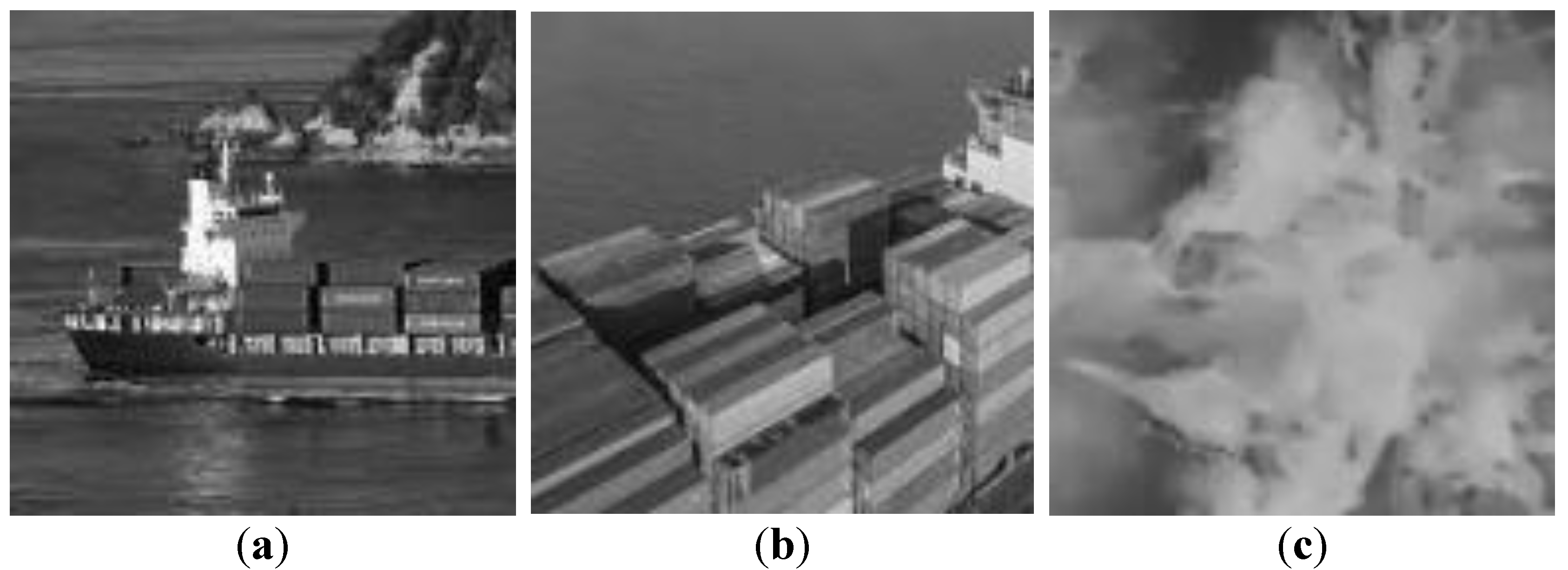
Figure 2.
Sequence of a region-based detection algorithm .
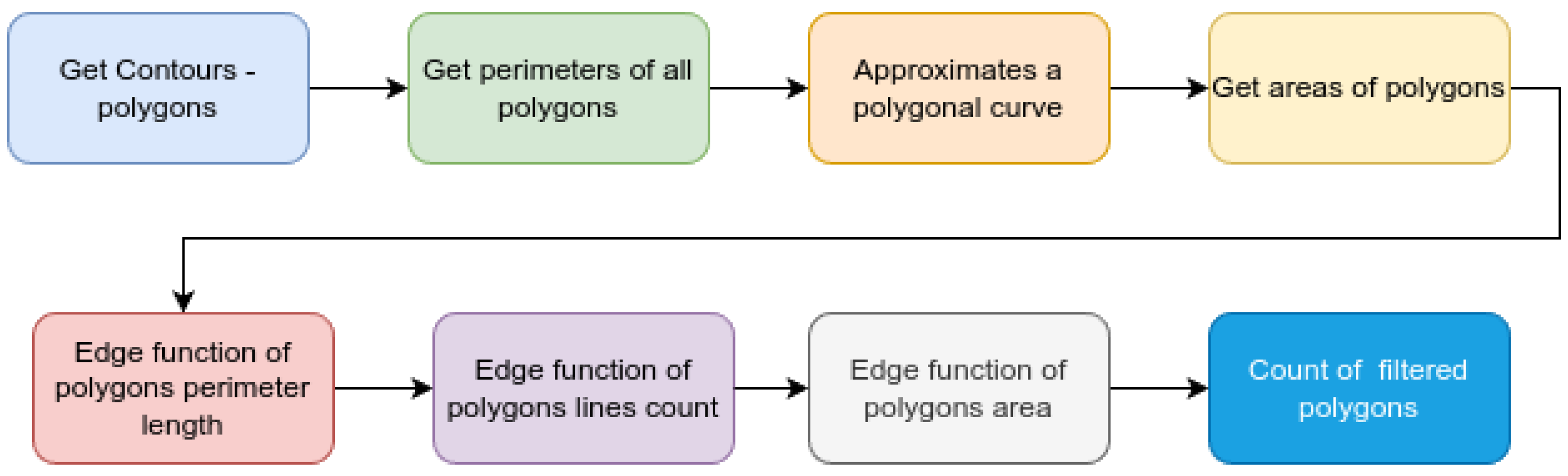
Figure 3.
Components of the artificial neural network.
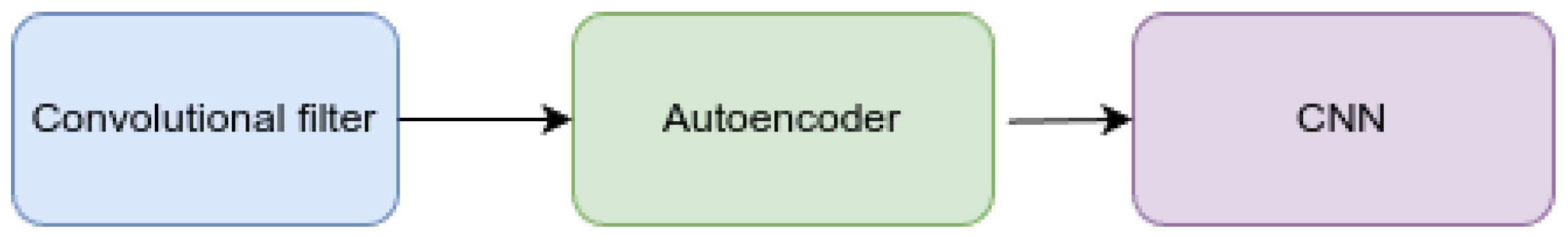
Figure 4.
The convolution filter used with dimensions 3x3 and respective parameters.
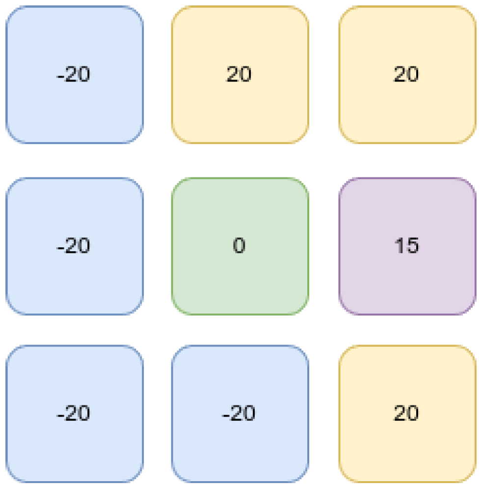
Figure 5.
Result of a convolutional filter applied to an image. (a) - grayscale input image, (b) - same image after the application of the convolutional filter.
Figure 5.
Result of a convolutional filter applied to an image. (a) - grayscale input image, (b) - same image after the application of the convolutional filter.
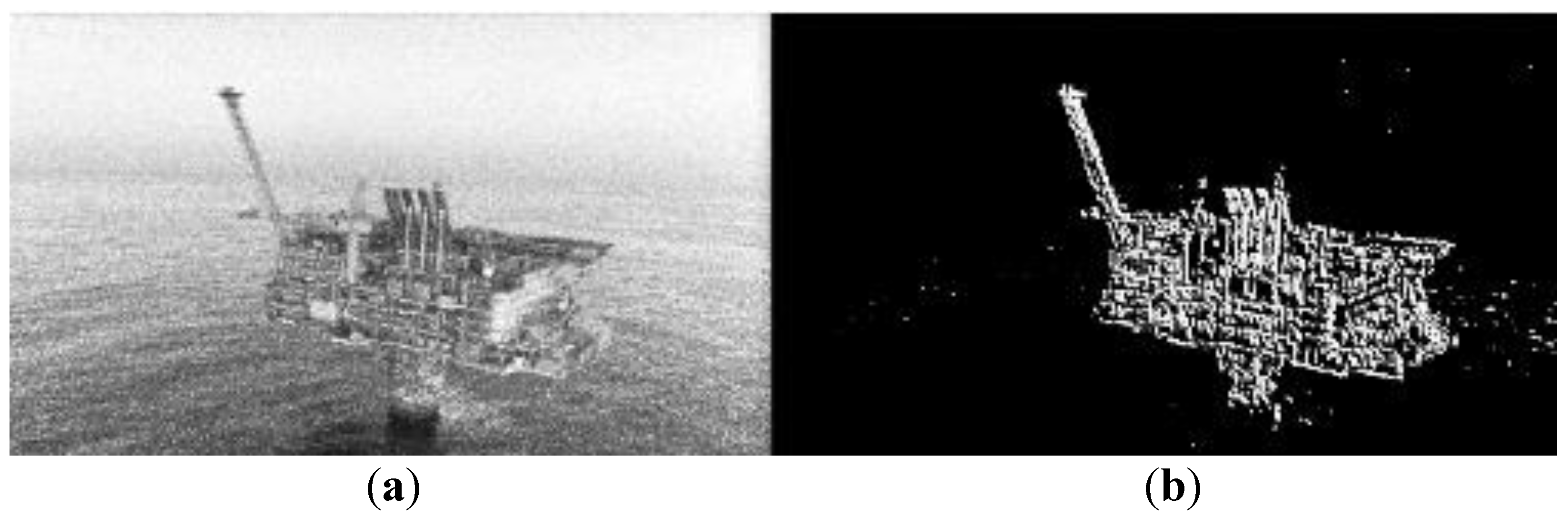
Figure 6.
Classic autoencoder architecture.
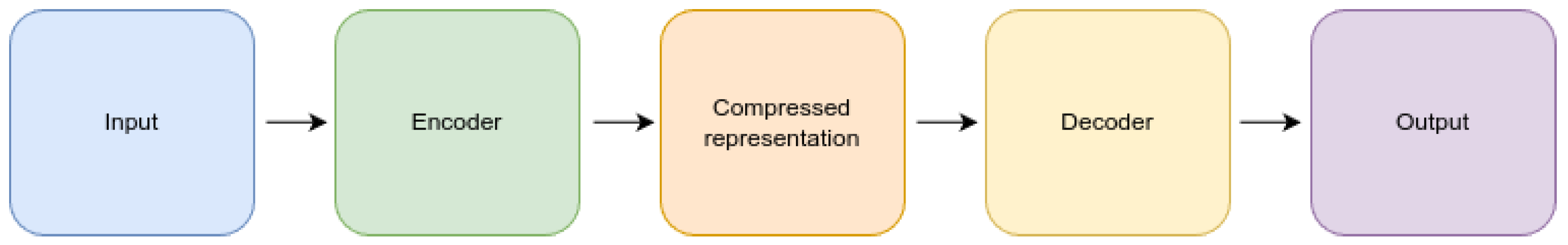
Figure 7.
CNN hyperparameter iteration cycle structure.
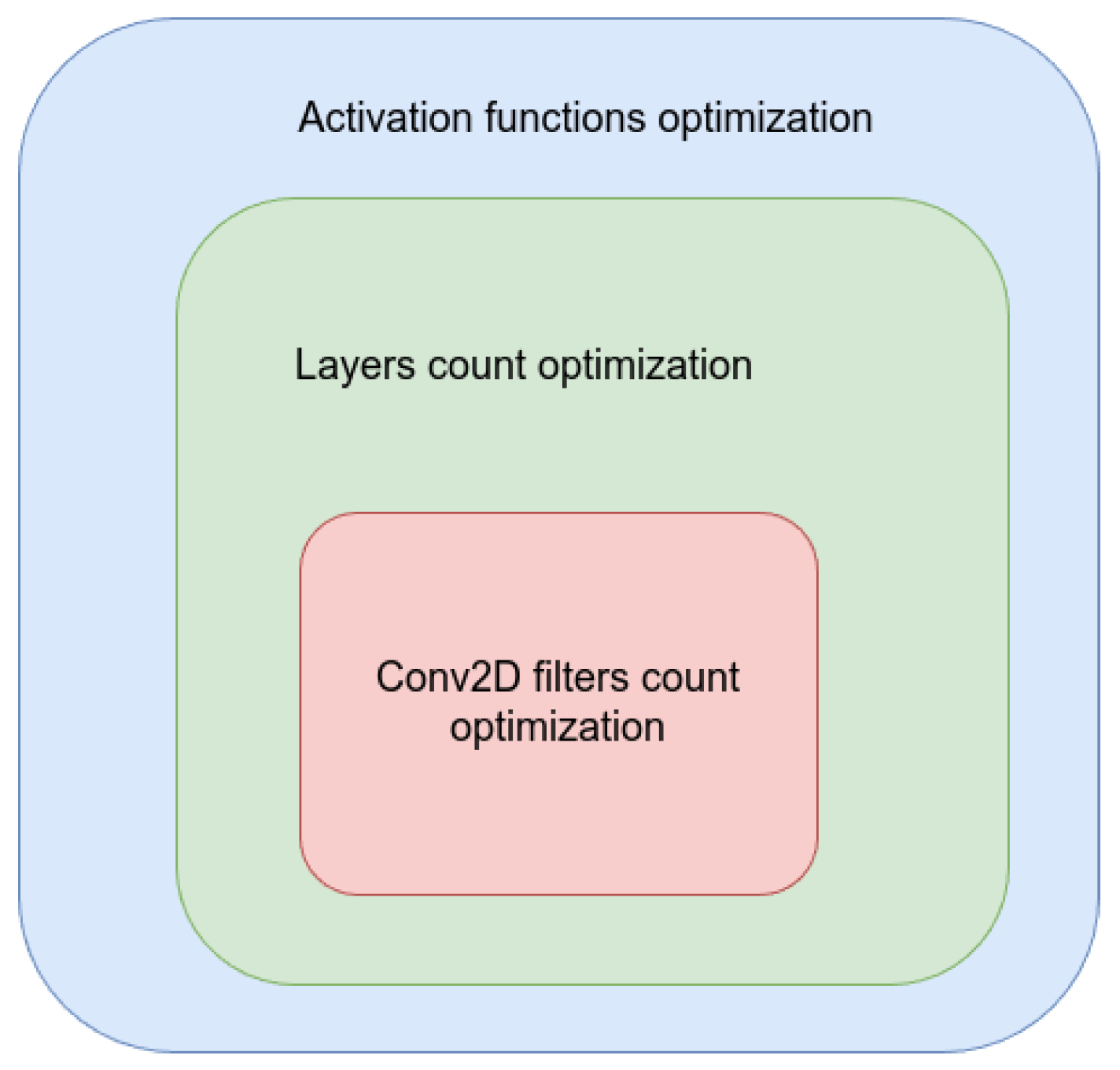
Figure 8.
UAV search mission schematic Every frame is used for detection, which is performed by two algorithms simultaneously. The region-based method is responsible for detecting objects of appropriate size and complexity, while the CNN-based method is responsible for detecting man-made patterns. .
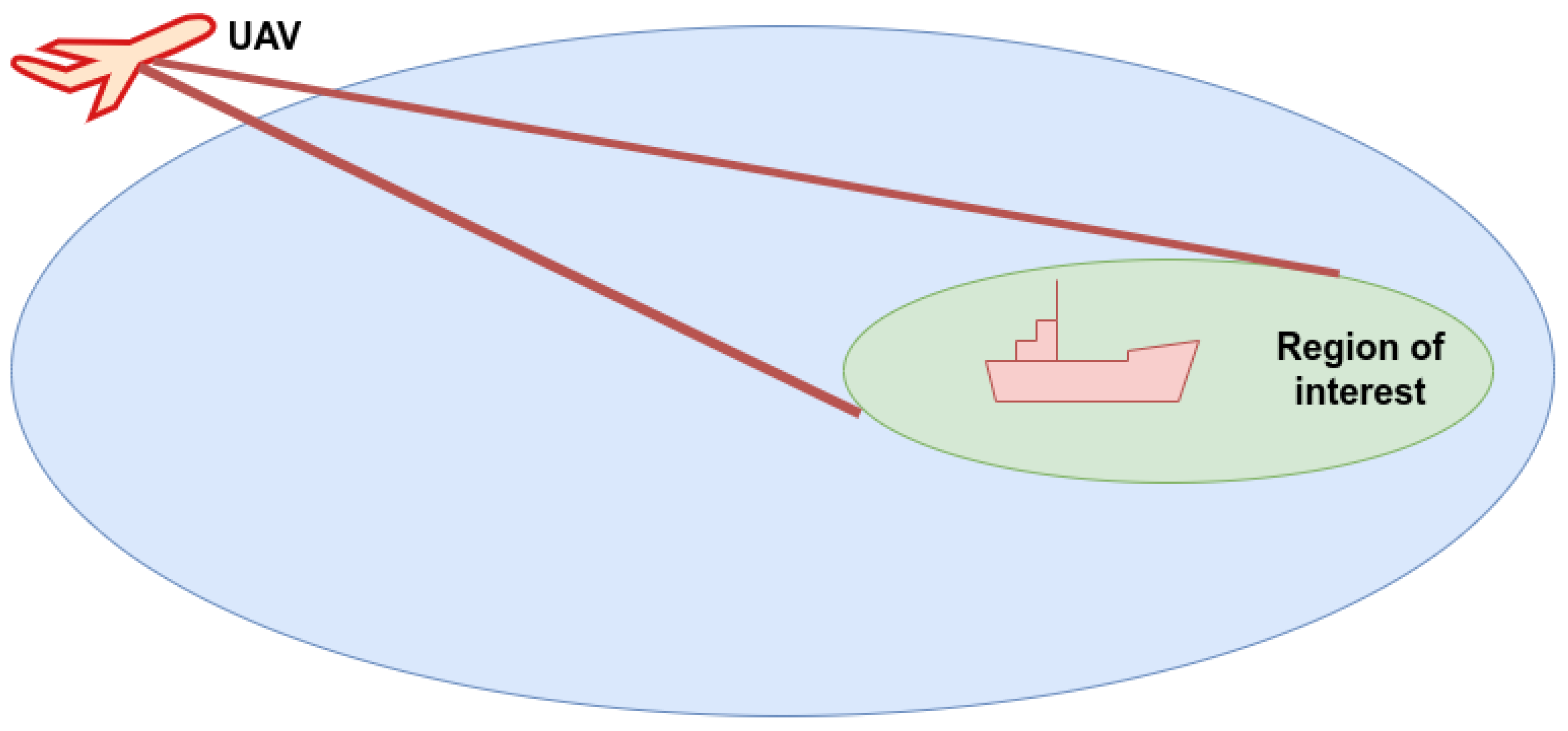
Figure 9.
Diagram of the proposed detection and tracking algorithm .
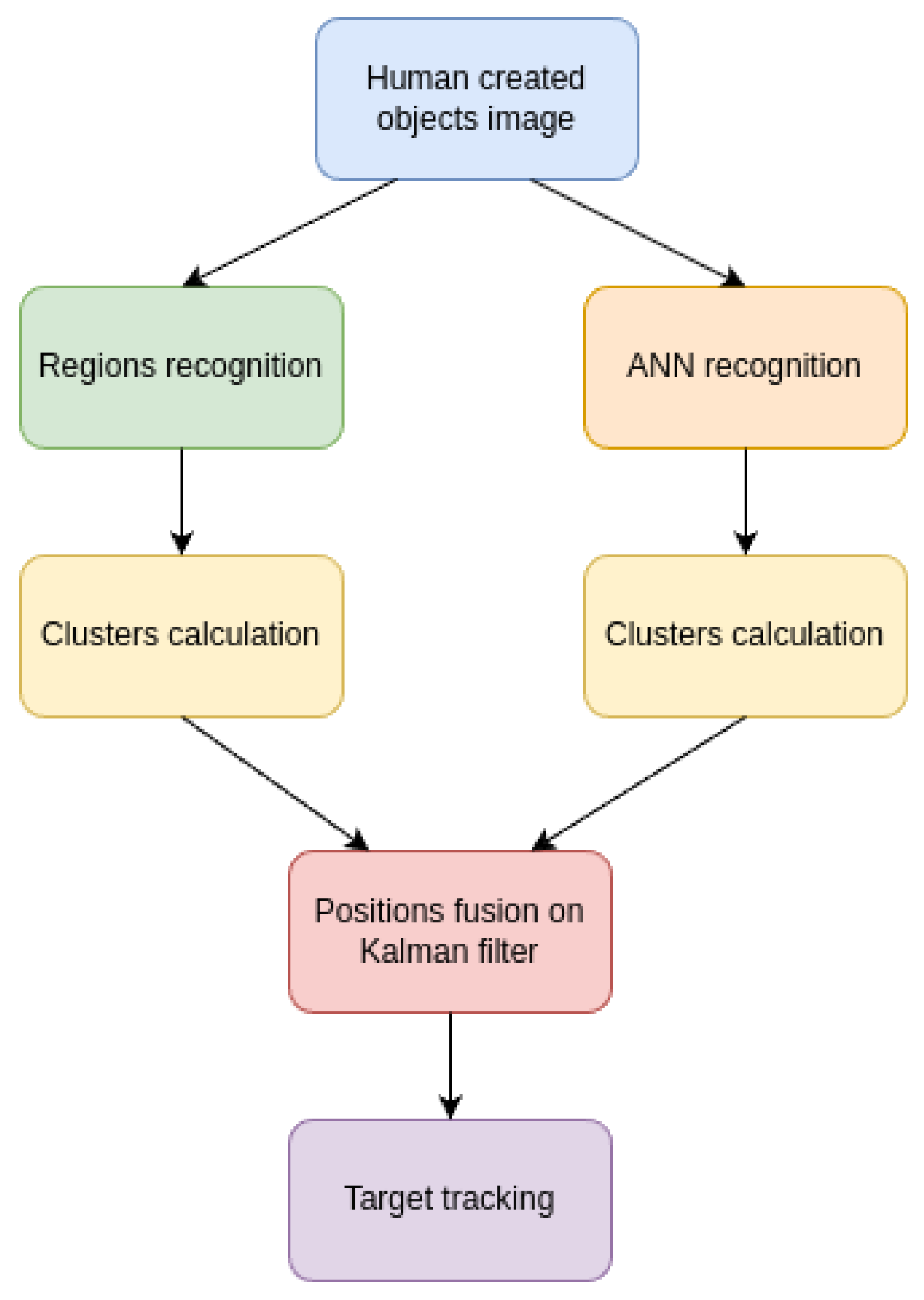
Figure 10.
ANN-based algorithm training performance diagrams.
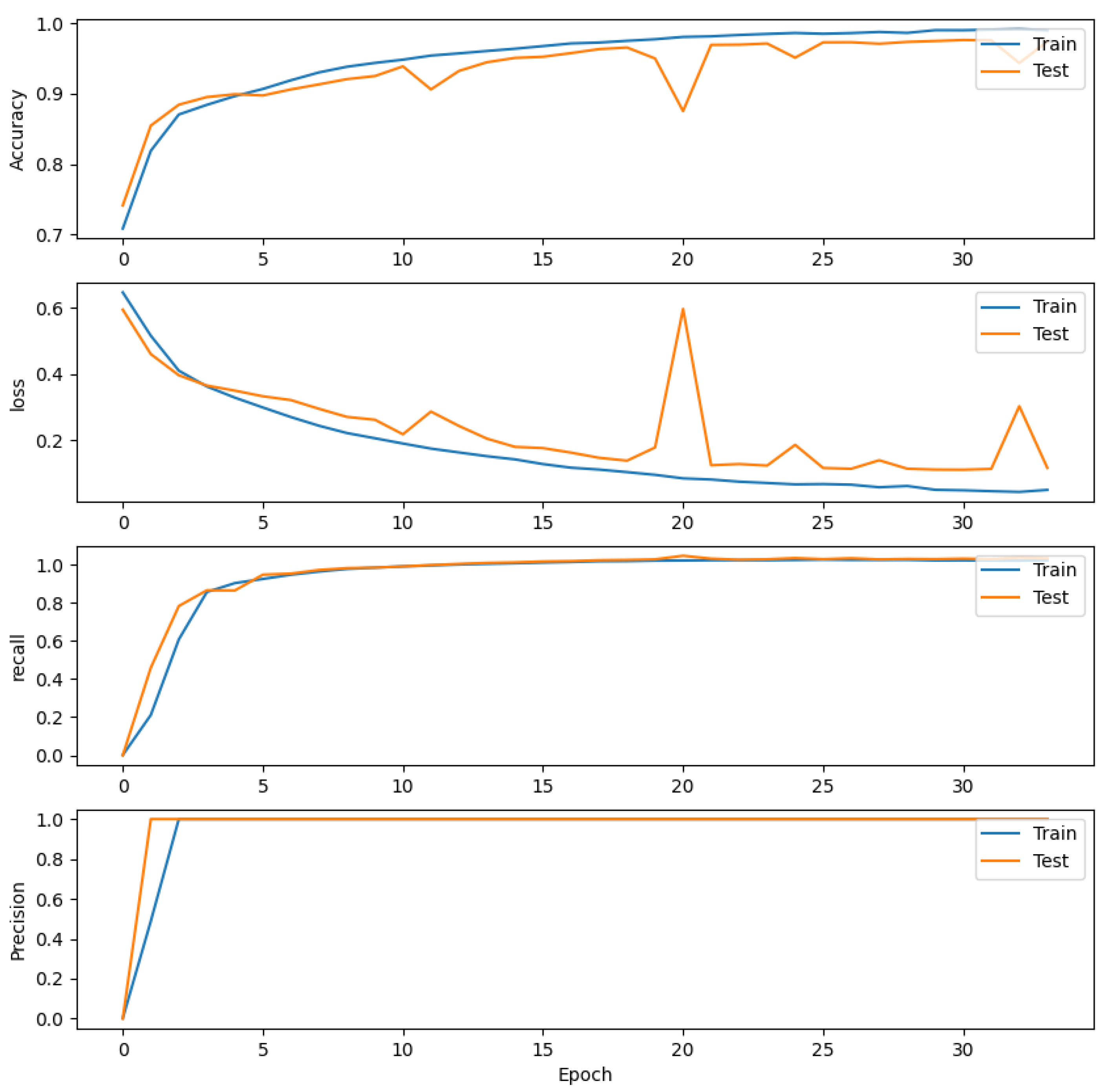

Table 1.
A list of aerospace-based datasets, containing marine objects .
| Dataset | Platform | Angle Range |
|---|---|---|
| [23] | Simulated satellite | 90° |
| Airbus Ship [24] | Satellite | 90° |
| NWPU VHR-10 [25] | Satellite | 90° |
| NWPU RESISC45 [26] | Satellite | 90° |
| HRSC2016 [27] | Satellite | 90° |
| FGSD [28] | Satellite | 90° |
| SeaDroneSim [22] | Simulated drone | 0 − 90° |
| DOIR [29] | Satellite | 90° |
| xView [30] | Satellite | 90° |
| SeaDronesSee [17] | Drone | 0 − 90° |
Table 2.
Tested Canny threshold values with respective mean pixel values on the positive and negative datasets.
Table 2.
Tested Canny threshold values with respective mean pixel values on the positive and negative datasets.
| Low threshold | High threshold | Negative mean | Positive mean |
|---|---|---|---|
| 50 | 100 | 13.99 | 26.17 |
| 100 | 150 | 8.42 | 17.77 |
| 150 | 200 | 5.07 | 13.22 |
| 200 | 250 | 3.07 | 10.30 |
| 250 | 300 | 1.88 | 8.12 |
| 300 | 350 | 1.45 | 6.4 |
| 350 | 400 | 0.68 | 5.03 |
| 400 | 450 | 0.38 | 3.91 |
| 450 | 500 | 0.21 | 3.01 |
| 500 | 550 | 0.11 | 2.29 |
| 550 | 600 | 0.06 | 1.72 |
| 600 | 650 | 0.03 | 1.28 |
| 650 | 700 | 0.01 | 0.94 |
| 700 | 750 | 0.00 | 0.68 |
Table 3.
The ANN algorithm composition.
| Nr. | Layer type | Shape | Parameter count | Specific function |
General function |
|---|---|---|---|---|---|
| 1 | Rescaling | (128, 128, 1) | 0 | Rescaling | Preprocessing |
| 2 | Convolution | (126, 126, 1) | 9 | Edge detection | |
| 3 | Convolution | (126, 126, 32) | 64 | Autoencoder-like layers |
|
| 4 | Max pooling | (63, 63, 32) | 0 | ||
| 5 | Convolution transpose | (126,126, 32) | 1056 | ||
| 6 | Convolution | (126, 126, 32) | 1056 | Convolution core layer pairs |
Core layers |
| 7 | Max pooling | (63, 63, 32) | 0 | ||
| 8 | Convolution | (63, 63, 96) | 3168 | ||
| 9 | Max pooling | (31, 31, 96) | 0 | ||
| 10 | Flatten | (92256) | 0 | Output layers | |
| 11 | Dense | (4) | 369028 | ||
| 12 | Dense | (2) | 10 |
Table 4.
Confusion matrix of the region-based method, tested on different dataset combinations .
| Dataset combination | TP | FN | FP | TN |
|---|---|---|---|---|
| 1 | 1778 | 1308 | 373 | 2713 |
| 2 | 1834 | 1252 | 338 | 2748 |
| 3 | 1788 | 1298 | 353 | 2733 |
| 4 | 1809 | 1277 | 318 | 2768 |
| 5 | 1784 | 1302 | 339 | 2747 |
| 6 | 1772 | 1314 | 365 | 2721 |
| Average | 1794 | 1292 | 348 | 2744 |
Table 5.
Performance metrics of the region-based method, tested on different dataset combinations .
| Dataset combination | Accuracy | Precision | Recall | F1 score |
|---|---|---|---|---|
| 1 | 0.728 | 0.827 | 0.576 | 0.679 |
| 2 | 0.742 | 0.844 | 0.594 | 0.697 |
| 3 | 0.733 | 0.835 | 0.579 | 0.684 |
| 4 | 0.742 | 0.850 | 0.586 | 0.694 |
| 5 | 0.734 | 0.840 | 0.578 | 0.685 |
| 6 | 0.728 | 0.829 | 0.574 | 0.679 |
| Average | 0.734 | 0.838 | 0.581 | 0.679 |
Table 6.
Confusion matrix of the ANN, trained and tested on 6 combinations of datasets .
| Dataset combination | TP | FN | FP | TN |
| 1 | 2972 | 114 | 50 | 3036 |
| 2 | 3028 | 58 | 11 | 3075 |
| 3 | 3035 | 51 | 23 | 3063 |
| 4 | 3036 | 50 | 17 | 3069 |
| 5 | 3020 | 66 | 18 | 3068 |
| 6 | 3019 | 67 | 18 | 3068 |
| Average | 3018 | 68 | 23 | 3063 |
Table 7.
Performance metrics of the ANN-based method, tested on different dataset combinations .
| Dataset combination | Accuracy | Precision | Recall | F1 score |
| 1 | 0.973 | 0.983 | 0.963 | 0.973 |
| 2 | 0.989 | 0.996 | 0.981 | 0.988 |
| 3 | 0.988 | 0.992 | 0.983 | 0.988 |
| 4 | 0.989 | 0.994 | 0.984 | 0.989 |
| 5 | 0.986 | 0.994 | 0.978 | 0.986 |
| 6 | 0.986 | 0.994 | 0.978 | 0.986 |
| Average | 0.985 | 0.992 | 0.978 | 0.985 |
Table 8.
Performance comparison of the algorithms tested.
| Algorithm | Accuracy | Precision | Recall | F1 score | Frame rate, Hz |
| Fusion-based ANN (ours) | 0.986 | 0.988 | 0.978 | 0.985 | 36.9 |
| Region-based detection (ours) | 0.734 | 0.838 | 0.581 | 0.679 | 142.9 |
| Simple CNN | 0.929 | 0.907 | 0.957 | 0.931 | 36.0 |
| MobileNet | 0.971 | 0.964 | 0.979 | 0.971 | 24.7 |
Disclaimer/Publisher’s Note: The statements, opinions and data contained in all publications are solely those of the individual author(s) and contributor(s) and not of MDPI and/or the editor(s). MDPI and/or the editor(s) disclaim responsibility for any injury to people or property resulting from any ideas, methods, instructions or products referred to in the content. |
© 2025 by the authors. Licensee MDPI, Basel, Switzerland. This article is an open access article distributed under the terms and conditions of the Creative Commons Attribution (CC BY) license (http://creativecommons.org/licenses/by/4.0/).
Copyright: This open access article is published under a Creative Commons CC BY 4.0 license, which permit the free download, distribution, and reuse, provided that the author and preprint are cited in any reuse.


