Submitted:
17 February 2025
Posted:
18 February 2025
You are already at the latest version
Abstract
It has great importance in maritime surveillance in preventing illegal activities and safeguarding oceanic operations. However, the conventional processes for ship detection fall under an inefficient category because they depend highly on manual monitoring. This study explores deep learning, particularly Convolutional Neural Networks, for the automation of detection using satellite images. A custom CNN model was designed and trained on a publicly available dataset to classify images as "ship" or "no-ship." The architecture consists of convolutional and max-pooling layers for feature extraction followed by dense layers for classification with dropout techniques to prevent overfitting. Data augmentation techniques were used to improve the generalization of the model. The model achieved an accuracy of about 86%, which is promising for real-world maritime surveillance applications. Further improvements, including hyperparameter tuning and better balancing of the dataset, could give even better performance. The results confirm that the CNN-based ship detection method represents a promising way to automate ocean monitoring, thereby improving the accuracy and efficiency of maritime security operations.
Keywords:
CNN-based ship detection method
1. Introduction
The world's oceans currently constitute huge, mainly unpoliced stretches are maritime security and environmental safety. The World Bank (2022) cites estimates of nearly 20,000 human trafficking cases occurring every year via the sea, a large portion of which is due to the lack of tracking for the vessels. Alarmingly, around seventy-five percent of all industrial ships move through the common waters without any adequate monitoring, and mostly uncontrolled sectors easily fuel illegal activities like smuggling, human trafficking, and unlicensed fishing (Paul, 2024). Considering the size of ocean areas involved and the limitation of manual surveillance, automation in ship detection is very likely to present a more viable and reliable alternative [1,2,3].
Recent advancements in AI, especially deep learning and computer vision, make ship detection increasingly of utmost importance for maritime operations. Techniques such as Convolutional Neural Networks have shown extraordinary competency over the years in processing both aerial and satellite photographs for the identification of vessels and greatly enhance surveillance, navigation, and security. One such unfortunate instance, which points out the dire requirement of a robust ship detection system, occurred in Japan in 2020 when a bulk carrier leaked 4,000 tons of oil into an endangered coral reef region, resulting in damage that could not be undone (BBC, 2020). The tragedy could have been avoided if the ship had been detected and tracked in advance, and contingency operations undertaken [4,5,6,7,8].
The present study aims to develop an AI-driven system to detect ships using a convolutional neural network (CNN) that classifies satellite images as containing a ship or not. A frame with labeled ship detection data from Kaggle is used to train and evaluate the CNN model, targeting optimizing accuracy and computational efficiency. This research will also tackle other challenges associated with designing CNN models: data imbalance, overfitting, and limitations on feature extractions that hinder their applicability in real-world scenarios. The outcomes of this research will pave the way toward enhancing maritime surveillance, which will ensure a much safer, safe, and efficient monitoring of waterways across the globe [9,10,11,12]. In recent years, deep learning techniques have emerged as a powerful tool for automating complex tasks across various domains. These models, particularly Convolutional Neural Networks (CNNs), have shown significant success in applications ranging from medical image analysis, such as the detection of COVID-19 through chest X-rays [22], to image processing tasks involving energy-efficient designs for field-programmable gate arrays (FPGA) [23]. Additionally, machine learning approaches have been effectively used for cybersecurity applications, including the mitigation of attacks in networking protocols [24] and the prediction of link structures in criminal networks [25]. These methods are also expanding into sentiment analysis and IoT security, demonstrating their versatility in fields like financial news sentiment classification [29,30], DDoS attack detection [26], and ransomware prevention [27,28]. The adaptability of deep learning and machine learning models across such diverse areas emphasizes their potential in automating complex systems, improving efficiency, and providing novel solutions to longstanding challenges [31].
2. Architecture
2.1. Layer Sequence
The architectural making of a project is the crux of a model. That is why our team took time to analyze our choices in layers and ended up with something balancing being computationally fast while at the same time being intricate in the evaluation as shown in Figure 1.
Convolutional layer
We used a convolutional layer as it extracts important features from the input image by identifying patterns like edges, corners, and textures. It focuses on the spatial hierarchy of images while extracting features from raw input images. In the first layer, low-level features are detected (32 filters) from the shape (150x150) while in the second layer main purpose is to detect mid-level features (64 filters) [13,14,15,16,17,18]. The kernel size is 3x3 through the input image in dot product between the kernel and values to create a feature map. The reason why two convolutional layers were used is to extract more diversity in features, having one pick up on larger features and another on smaller ones. This was supported by several tests for different feature sizes, and our team agreed on this version as seen in the epochs that the accuracy was in an excellent range [18].
MaxPooling2D, Pooling Layer
This layer enables spatial dimension reductions of the input images to the down sample by applying a window feature map to prevent overfitting and extract vital features while max pooling that can replace the image even if they are changed slightly. For the kernel size, 2x2 is commonly used since it reduces dimensionality in half. It is placed after every convolutional layer to ensure that the data is well taken care of in terms of load and retaining information effectively. Dense layer After the data transitions from 2D to 1D through the flattened layer, it sets foot to the dense one. This layer is responsible for combining features from the previous layers like the pooling and convolutional to enable decision-making for the classification model. The number of neurons has been set to 256 to determine the dimensionality of the output and to avoid underfitting and overfitting, the output layer has been selected as SoftMax for multi-class classification, and it converts the outputs into a probability distribution. The first layer combines the features from the previous layer and the second layer refines the complex features [19].
Dropout
Then it was put between the two dense layers as a dropout regularization to prevent overfitting in its work, as it can drop some neurons when training to force the model to depend on a big variety of features rather than depending on specific neurons during feeding forward. The 0.5 is the standard for dropout layers since it drops 50% of neurons and is good because prevents overfitting in large networks [20].
Numerical Rationale
The architecture selected for this CNN model was computed to be a detailed and efficient approach. The aim was to design a framework that is not entirely redundant to increase the amount of run time or too general and causes overfitting but would suffice enough to be able to refine the model effectively.
We didn't want to follow the conventional procedure blindly and tried to find specific solutions. During our model testing, we found out our model performed better when extracting with smaller standard convolutional kernels. To validate this, we ran a few tests based on the initial accuracy of the model as shown in Figure 2 [21].
The above output was taken from a (11, 11) kernel size convolutional layer. This size would take up to 1/5 of the image and detect more complex features. Clearly, the accuracy is extremely low and wouldn't suffice in creating a working model as shown in Figure 3.
The above output is based on a (3, 3) convolutional kernel size which significantly increases the initial accuracy of the model. Because of this, we have settled on a smaller kernel size. We further investigated our findings and came to realize that perhaps the larger size kernels had caused an extreme increase in parameters in the model, making it harder to arrive at a specific result in training. This could have also possibly caused a bout of overfitting. Therefore, we settled on the more standard approach: (3, 3) as shown in Figure 4.
We noticed that our specific dataset had differences on both a medium and smaller level, as in it required an architecture that supported looking at details that aren't as extremely complicated as a dataset that would identify high-resolution images and not as general as one identifying pure shapes. We settled on a model that would pick up the shape of ships apart from their more common details. After feeding the input image using 'input shape' with a size of 150x150 pixels to keep many details over the full 3 RGB colors, the model was built using two convoluted and pooling layers because that showed the optimum performance of the model with two layers and any more did not produce any good results. The filter of the first convolutional layers was put to 32 to pick up on normal features, later boosted to 64 for the second one to predict more complex ones. The size of the filter was set to (3,3) both methods capture finer details in the dataset. Generally, the pooling layers were set to (2,2) and put after every convoluted layer to reduce half of the dimensions extracted and reduce the load against overfitting as shown in Figure 5.
A flattened layer was then used to condense the 2D matrix to a 1D to integrate the found data into the dense layers. A dense layer was applied afterward to further train the model on more complex features, now with 256 neurons for further optimized learning, with the ReLU activation function used for its simplicity and performance. A dropout of 0.5-layer acts in between the two dense layers dropping a few images from the database and making the model confront overfitting by forcing it to learn diverse neuron pathways. The final dense layer was subsequently added with 2 neurons representing the database's two classes 'ship' and 'no ship' along with a SoftMax activation function used for its classification capability.
3. Implementation
3.1. Setting Up Environment and Loading Data
In this phase, we set up the environment and loaded the dataset for the ship classification task. The required libraries such as TensorFlow and some utilities needed for image processing are imported. Google Colab is used for mounting Google Drive to be able to access the dataset present there. We use the Image Data Generator from TensorFlow for applying data augmentation on the images in real-time. This is done to prevent overfitting and improve the model generalization performance through transformations such as rotating, shifting, zooming, etc., as shown in Figure 6.
3.2. Data Preprocessing with Augmentation
Data augmentation is an integral part of the deep learning workflow, artificially boosting the number of datasets, principally to mitigate the feel of overfitting while simultaneously enhancing model generalization. Due to the small dataset size of images for the shipping category, transformations including rotation, width and height shift, zoom, and horizontal flipping can harden the model against different realistic variations in the data.
We first create a dataset directory, ‘dataset_dir’, to use later on. Then came the time to deploy the data generator for augmentation of the data. Next, parameters were set, beginning with ‘rescale’-the normalization process. The validation split was then issued at 30% in deviation from an 80/20 rate for the given case, to allow in-depth validation of such data. Finally, the images underwent all kinds of augmentation: rotation, horizontal and vertical shifts, shearing, zooming in, and flipping. To fill in the missing pixels caused by any change to an image an image generator has made, we set a fill mode to stretch the nearest pixel near a gap.
Then training and validation data have been loaded. We used the directory path created earlier to map to our dataset. The image size was kept at 150x150 pixels just enough to take details without being computationally inefficient. The batch is set to 32 because it fits well into a standard GPU memory and had a more stable run without causing the model to break due to RAM overload. The output of the model is in a format where classes belong to categories, hence we set it for classification in categorical mode. Although binary classification would generally have proven very efficient at this point since it is more specialized for binary classes, surprisingly, categorical classification gives an overall better accuracy. For safety, therefore, we went ahead and used this categorical classification. The subset parameter defines whether the code is being run for training or validation.
Dataset Splitting
The dataset has been partitioned into two main subsets: training and testing. This division is essential for assessing the model's capacity to generalize and accurately predict outcomes with previously unseen data. A split ratio of 70% for training and 30% for testing has been selected.
Justification for the Split Ratio
The 70-30 distribution is commonly employed in machine learning, as it strikes a balanced approach that provides ample data for both training and evaluation. The larger portion earmarked for training allows the model to learn from a wide range of examples. Conversely, the test set constitutes 30% of the total data, which is significant enough to yield reliable insights into how the model might perform in actual applications. Additionally, this ratio aids in detecting potential problems such as overfitting or underfitting since performance assessments are conducted on unseen data not utilized during training. Although some literature suggests an alternative 80-20 split (V. Roshan Joseph, 2022), where 80% of data serves as input for training and only 20% acts as a testing subset guided by the Pareto Principle (often referred to as the 80/20 rule), such an arrangement may occasionally fall short when aiming for a nuanced understanding of model performance. The selected 70-30 split embodies a more tailored strategy designed to facilitate deeper and more precise evaluations of model behavior. By allocating one-third of their available data toward testing, models are subject to more stringent scrutiny, thereby enhancing the trustworthiness of evaluation metrics while providing stronger insights regarding their generalization abilities.
3.3. Data Visualization
Verification steps generally include visual inspection of data before model training. The code below retrieves a batch of images and their related one-hot labels from the training set. As output, the screens display a 5 x 5 arrangement of images along with their class label ("ship" or "no-ship"), which is obtained from the one-hot encoded vector. Evidently, as part of the EDA, it is crucial to inspect our data first to check for any anomalies. We set our class names in a list, then load a batch of images along with their labels from the train generator using a next pointer. Then we use matplotlib to create a figure of size 10x10. This will iterate through the list, using 25 images and placing them on a 5x5 plot. The images will increment their index by 1 to make iteration easier. The class names must be reassigned after using labels. The labels are binary in format, so we use argmax to find the maximum value, which is 1. Then we use these labels to index the class names list. The names are assigned back to the variables automatically; no-ship is at the starting zero index and ship at one. The rest of the code is about the figure aesthetics, such as toggling ticks and grids off, and then showing the images in the plot as shown in Figure 7.
CNN Model Architecture
Next addressed is the architecture of the Convolutional Neural Network (CNN). The model begins with two convolutional layers, with the max-pooling layers being inserted for feature extraction and dimensionality reduction. The last dense layer provides two outputs, namely ship or no-ship class probabilities, via using the SoftMax activation function. A dropout layer was added to lessen the effects of overfitting. For model architecture, we imported the layers required and then decided to work in sequential mode since models are linear stacks of layers. According to the architecture diagram, we chose the 3x3 kernel for all the convolutional layers, for the first convolutional layer with a depth of 32, to extract simpler features, while the next was at 64 depths for deeper, more complex features. The input image was set to 150x150, since it had 3 RGB colors, after the first conv_2D layer. This 150x150 input is supposed to be used for all layers though the convolutional and the max-pooling ones do change the input size, where the convolutional layer shrinks it down to 148 in one go simply by taking out two pixels from either corner, which is again halved to 74 after max pooling, etc. The max pooling function was used to extract dominant features and reduce spatial dimensions. Since the smaller kernel sizes tend to combat overfitting, we made it into 2x2 for max pooling to fully employ it. To not sound repetitive in this section on architecture, we can go ahead with model compilation. Using the Adam optimizer turned out to be quite effective and robust in comparison with other optimizers, particularly for our datasets with respect to efficiency and learning rates. Later on, binary_crossentropy was selected to cope with training the model with the dichotic classes of ship and no ship. Finally, since machine learning algorithms train for a particular task based on a specific metric, we will define our metric as accuracy, the very parameter we want to measure. Then, we gave the model a summary to see a simple table of our layers along with their information.
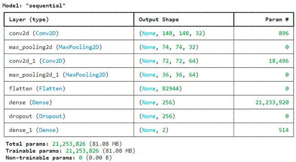
Output Snippet: The model summary outputs the number of parameters in each layer, highlighting the complexity of the model. The model consists of over 21 million trainable parameters, indicating a sophisticated network capable of learning intricate patterns from the data.
To help us visualize our layers, we also used AlexNet representation for additional insights. We can visualize the model architecture by calling the plot Model function. Set show shapes to True to display input and output for each layer and give a visualization of the dataflow between the layers. True was also set for show_layers_names, which will show the name of each specific layer.
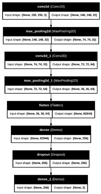
The data flow and the dimensions associated with the input and output shapes are climatically shown along the provided layer names. Note that each output is fed into the subsequent layer. The initial input size was 150 by 150 but becomes 148 by 148 after the Conv layer takes away two pixels, and after that, the max-pooling layers shrink it to half of the input size. This continues until they reach the flattening of pixels into a 1D output. Dense then condenses the data, and Drop removes some neurons to avoid overfitting before the final dense in which the data is condensed into two classes our ship and no-ship class as shown in Figure 8.
Training the CNN Model:
Training of the Neural Network would consist of the repeated handling of the training data and the adjustment of the model weights to minimize the loss function. The model is trained for 10 epochs, which offers a good representation of hyperparameters wherein the model is exposed sufficiently to the data, while the computational cost stays within limits. In training, we provide the training data to the network, and the weights are then adjusted using backpropagation, where the model learns to reduce the error through iterative updates. Validation data, which the model has not encountered during training, was monitored after each epoch for model performance. This information provided a measure of the model's ability to generalize beyond training data.
Performance Evaluation and Visualization
Model Accuracy
At the end of the training procedure, one evaluates the accuracy of the model on the validation dataset, and the training and validation accuracies over epochs are plotted to visualize the learning progress of the model. Subsequently, when testing on the test set, one calculates the test accuracy and loss.
Figure 9 shows the test accuracy of the model at 83.50% shows its effectiveness in distinguishing images of the "ship" and "no ship" classes. In such a case, the performance shows that the model generalized quite well when applied to unseen data.
Confusion Matrix and Classification Report
The confusion matrix and classification report further provide insight into the performance of the model. To discuss it in a bit more detail, the confusion matrix serves as an index whereby one observes the true positive, true negative, false positive, and false negative values as to how the model performs for each class. Whereby, the classification report gives the following metrics: precision, recall, and F1-score.
Figure 10 indicates the confusion matrix along with the classification report gives detailed information on how well the model performs for both classes. Precision, recall, and F1-score for each class are given, which shows that the model is slightly better in the precision of the "no-ship" class, while on the other hand, the "ship" class has a relatively lower recall but overall performs well.
Evaluation of Testing Set:
Once training is done, the last step would be to evaluate how the model performs on the testing dataset, a set that it has never seen in its training phase. This is an important step for analysing how well the model generalizes. After testing, the model achieved a test accuracy of around 85%. This score describes the capacity of the model to predict the probability of the presence of a ship or not in test images. Test loss is the difference between the predictions and actual labels. The lesser the test loss, the better it is because that means the predictions of the model are closer to the true labels.
Confusion Matrix and Classification Metrics:
Other evaluation metrics are made, including a confusion matrix and classification report, to have a deeper look into how the model performs. The confusion matrix is a visual representation of the model's predictions, with true positives, false positives, true negatives, and false negatives being highlighted. This matrix can be used to diagnose how well the model is distinguishing between classes. A detailed classification report that gives metrics includes precision, recall, and F1-score. Precision tells how correct the positive predictions are, while recall is how good the model is at detecting positive cases. The F1-score is the harmonic mean of precision and recall; thus, it balances the metrics of performance for better evaluation when there are imbalanced classes. For instance, it may provide higher precision for the "no-ship" class, which explains that it is more precise when the prediction is about "no-ship" images. However, the recall of the "ship" class might be slightly less, which means that the model occasionally misses some images of ships but still performs acceptably.
Conclusion
Ship Detection Our aim in this project was to build a CNN model that could detect ships to monitor the oceans more efficiently, thus preventing illegal activities, and providing automated monitoring capability over edges of the manageable aquatic areas. Ship detection was the goal of the fusion of two datasets which has been created to support automatic ship detection. The training-validation metrics were regularly evaluated to facilitate the best possible learning without overfitting. To have learned the intellectual performance of the configuration, additional augmentations and dropout added. As presented, the findings show that the test accuracy stands at 86.5%, which denotes the capability of the model to prove the true classification of the classes’ 'ship' and 'no-ship'. Additional detailed analysis in terms of the classification report and confusion matrix further revealed that the model detected 'no ship' classes more efficiently - which shows corroborating evidence for the greater precision of that class Whereby, this project has successfully applied a CNN model in satellite images for the detection of ships, thereby representing how solving real-world problems is achievable via deep learning techniques. All decisions regarding data augmentation, architecture building, and evaluation methods were carefully defended and critically evaluated. The model is likely to improve further, with more optimizations in the future like hyperparameter optimization or supplying new data, allowing for more sophisticated use in the field of satellite image interpretation.
Challenges Faced
The project was characterized by various challenges that included problems relating to imbalanced data. The class of no ships had images that had a considerable imbalance of having more images than the ships themselves. This led to establishing bias in the model that distorted the outcomes. To mitigate this challenge, we have decided to combine two datasets from Kaggle to balance the ship class. The second issue was the model which suffered from overfitting, in which the validation accuracy surpassed the test accuracy. After many headaches with thorough searching of different literature, this issue was finally conquered by introducing the dropout layer. Then the standard versus exploration dilemma came. Our team was keen on getting the best research of code and standards; however, not every writing on CNN solutions fitted our specific model. That again forced us to develop some time and error techniques for pinpointing the right configurations for our model. Ultimately, we thought our iterative approach helped in overcoming those challenges and improving our model performance to a considerable extent.
Figure 11 shows the model evaluation; we chose accuracy measurement for an overall assessment of test loss. This model seems to generalize well to unseen data. We expect the validation accuracy to be smooth along the train plot with the gist of being inferior. The graph above indicates that while not passing on validation accuracy with a continuous loss of 0.35, the near approximation to training accuracy can suggest the model is functioning well and can adapt to new data at a considerable pace. Hence shortly, of course, this can improve on matching training accuracy, but with a current test accuracy of 86%, a fair part of the data has been identified correctly.
As a result of checking whether or not the model performs well across all classes, the confusion matrix was attached as shown in Figure 12. The model is doing somewhat decently, giving a higher estimate of true positives and true negatives to compare with a false one, with around 699 and 513 cases correct for the no-ship class and ship cases respectively. However, given that the no-ships class has a larger number overall, about 813 images, in comparison to the total 605 for ship images, this may give rise to some bias. Notwithstanding, this bias was taken care of as much as possible, seeing that the original dataset was skewed, with over 4k images of no-ships against just 2k ships. Our group scaled down the dataset to a more reasonable ratio by adding more ship images. Although still not equal, the confusion matrix certainly certainly has improved on what it used to be at the start of this project.
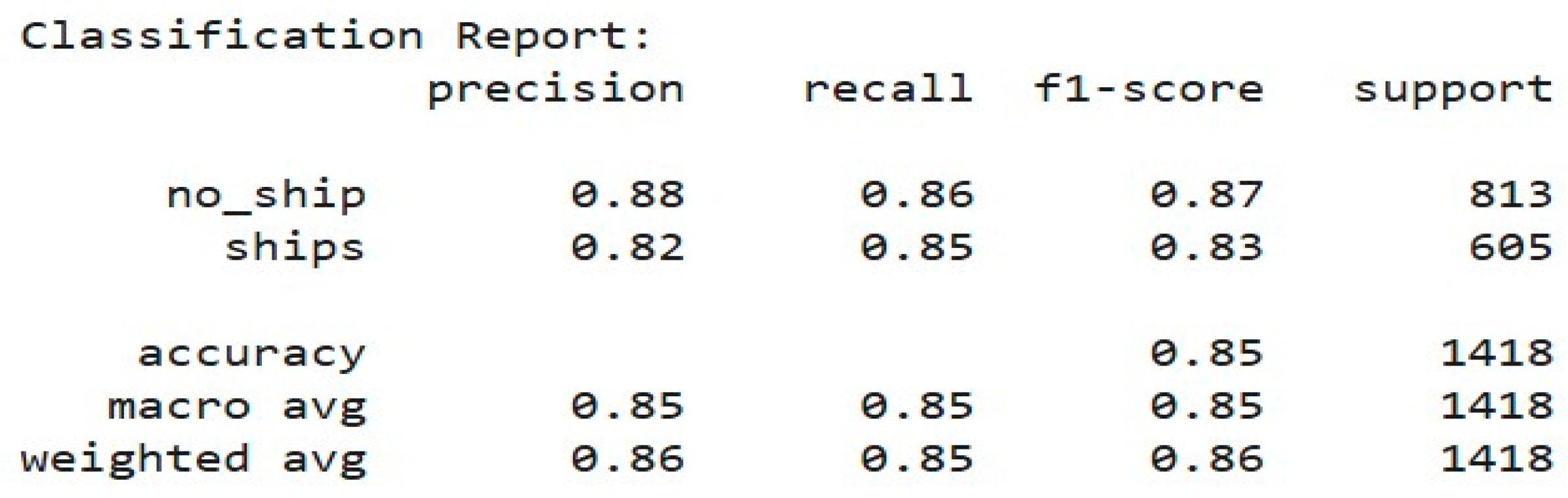
Lastly, as a feed of overall model performance, we generated a classification report to find key metrics like precision and recall. The scores were 0.87 f1 for no-ship and 0.83 for ship respectively, which highlighted the effectiveness of the model for making competent predictions for each class. However, it suffers from lower recall and greater precision on the no-ship class because this is much of the dataset, and it is more likely to be predicted as positive than to be recalled as negative but vice versa for the ship's class as shown in Figure 13.
Future Enhancements
While it has worked great for this model, there is still a lot to learn for future work. For instance, one thing learned is the quality of the dataset into which we have collected what we have decided to base on this study the interest of ship detection subject to our effort to solve marine surveillance problems; however, in the future, it should be considered balancing the number of images in the classes of a dataset to avoid biases in the process of training and validation. The other thing would be that, after getting all of that knowledge and experience, some in-depth image preprocessing and cleaning will be a very good consideration beforehand, like histogram equalization for better ship imaging and edge detection for improving shape detection; this will simplify the process of feature extraction into a more efficient model generalization of accuracy. The model may run just fine, but it is sure not ideal. There are quite a few experiences to learn from in the future project. One example of that is the quality of assessment of the data set. The choice made while creating this dataset was based on the subjectivity of interest in ship detection, together with our desire to find solutions to marine surveillance. The best to take on is not forgetting to balance the number of images of classes of the dataset so that no classes are left under or overrepresented during training and validation. Not to mention now with much more expertise and research after this project, it would be a valuable consideration to apply in-depth image processing and cleaning of images beforehand like histogram equalization for better image clarity of ships and edge detection for improving shape detection; thus, making efficient extraction of features much finer and boosting the general accuracy of the model.
References
- Aherwadi, N.; Mittal, U.; Singla, J.; Jhanjhi, N.Z.; Yassine, A.; Hossain, M.S. Prediction of Fruit Maturity, Quality, and Its Life Using Deep Learning Algorithms. Electronics 2022, 11, 4100. [Google Scholar] [CrossRef]
- Alferidah, D. K., & Jhanjhi, N. Z. (2020, October). Cybersecurity impact over big data and IoT growth. In 2020 International Conference on Computational Intelligence (ICCI) (pp. 103-108). IEEE.
- Alghazo, J., Bashar, A., Latif, G., & Zikria, M. (2021, June). Maritime ship detection using convolutional neural networks from satellite images. In 2021 10th IEEE International Conference on Communication Systems and Network Technologies (CSNT) (pp. 432-437). IEEE.
- Chen, Z.; Chen, D.; Zhang, Y.; Cheng, X.; Zhang, M.; Wu, C. Deep learning for autonomous ship-oriented small ship detection. Saf. Sci. 2020, 130, 104812. [Google Scholar] [CrossRef]
- Erbe, C.; Smith, J.N.; Redfern, J.V.; Peel, D. Editorial: Impacts of Shipping on Marine Fauna. Front. Mar. Sci. 2020, 7. [Google Scholar] [CrossRef]
- Jena, K.K.; Bhoi, S.K.; Malik, T.K.; Sahoo, K.S.; Jhanjhi, N.Z.; Bhatia, S.; Amsaad, F. E-Learning Course Recommender System Using Collaborative Filtering Models. Electronics 2022, 12, 157. [Google Scholar] [CrossRef]
- Joseph, V.R. Optimal ratio for data splitting. Stat. Anal. Data Mining: ASA Data Sci. J. 2022, 15, 531–538. [Google Scholar] [CrossRef]
- Mauritius oil spill: Wrecked MV Wakashio breaks up. (2020). BBC News. Retrieved from https://www.bbc.com/news/world-africa-53797009.
- Paul, A. (2024). AI and satellite data helped uncover the ocean’s ‘dark vessels.’ Popular Science. Retrieved from https://www.popsci.com/technology/ai-dark-vessels/.
- Qu, J.; Gao, Y.; Lu, Y.; Xu, W.; Liu, R.W. Deep learning-driven surveillance quality enhancement for maritime management promotion under low-visibility weathers. Ocean Coast. Manag. 2023, 235. [Google Scholar] [CrossRef]
- REDUCING MARITIME TRAFFICKING OF WILDLIFE BEST PRACTICES FOR PORTS. (2023). Retrieved from https://thedocs.worldbank.org/en/doc/7eb2120916bbf0e8b232749eb42b6519-0320012023/reducingmaritime-trafficking-of-wildlife-best-practices-for-ports.
- Saeed, S. (2021). Optimized hybrid prediction method for lung metastases. Artificial Intelligence in Medicine.
- Saeed, S., & Abdullah, A. Analysis of lung cancer patients for data mining tools. International Journal of Computer Science and Network Security 2019, 19, 90–105.
- Saeed, S.; Abdullah, A.; Jhanjhi, N. Investigation of a Brain Cancer with Interfacing of 3-Dimensional Image Processing. Indian J. Sci. Technol. 2019, 12, 1–6. [Google Scholar] [CrossRef]
- Saeed, S., & Abdullah, A. (2021). Combination of brain cancer with hybrid K-NN algorithm using statistical analysis of cerebrospinal fluid (CSF) surgery. International Journal of Computer Science and Network Security 2021, 21(, 120–130.
- Saeed, S.; Abdullah, A.; Jhanjhi, N. Implementation of Fourier Transformation with Brain Cancer and CSF Images. Indian J. Sci. Technol. 2019, 12, 1–9. [Google Scholar] [CrossRef]
- Saeed, S.; Abdullah, A.; Jhanjhi, N.Z.; Naqvi, M.; Nayyar, A. New techniques for efficiently k-NN algorithm for brain tumor detection. Multimedia Tools Appl. 2022, 81, 18595–18616. [Google Scholar] [CrossRef]
- Saeed, S., Khan, H. (2021). Global mortality rate and statistical results of coronavirus. Infectious Diseases and Tropical Medicine, 1-12.
- Saeed, S. Saeed, S., Naqvi, D. S. M. R., & Khan, H. A. Estimation of multi-crystalline photovoltaic cell using solar spectrum of five different bands. Life Science Journal 2016, 13, 56–61. [Google Scholar]
- Wang, Y.; Rajesh, G.; Raajini, X.M.; Kritika, N.; Kavinkumar, A.; Shah, S.B.H. Machine learning-based ship detection and tracking using satellite images for maritime surveillance. J. Ambient. Intell. Smart Environ. 2021, 13, 361–371. [Google Scholar] [CrossRef]
- Yin, Y.; Cheng, X.; Shi, F.; Zhao, M.; Li, G.; Chen, S. An Enhanced Lightweight Convolutional Neural Network for Ship Detection in Maritime Surveillance System. IEEE J. Sel. Top. Appl. Earth Obs. Remote. Sens. 2022, 15, 5811–5825. [Google Scholar] [CrossRef]
- Gouda, W.; Almurafeh, M.; Humayun, M.; Jhanjhi, N.Z. Detection of COVID-19 Based on Chest X-rays Using Deep Learning. Healthcare 2022, 10, 343. [Google Scholar] [CrossRef]
- Kumar, T.; Pandey, B.; Mussavi, S.H.A.; Zaman, N. CTHS Based Energy Efficient Thermal Aware Image ALU Design on FPGA. Wirel. Pers. Commun. 2015, 85, 671–696. [Google Scholar] [CrossRef]
- Zahra, F.T.; Jhanjhi, N.; Brohi, S.N.; Malik, N.A.; Humayun, M. Proposing a Hybrid RPL Protocol for Rank and Wormhole Attack Mitigation using Machine Learning. 2020 2nd International Conference on Computer and Information Sciences (ICCIS). LOCATION OF CONFERENCE, Saudi ArabiaDATE OF CONFERENCE; pp. 1–6.
- Lim, M.; Abdullah, A.; Jhanjhi, N.; Khan, M.K.; Supramaniam, M. Link Prediction in Time-Evolving Criminal Network With Deep Reinforcement Learning Technique. IEEE Access 2019, 7, 184797–184807. [Google Scholar] [CrossRef]
- Dogra, V., Singh, A., Verma, S., Kavita, Jhanjhi, N.Z., Talib, M.N. (2021). Analyzing DistilBERT for Sentiment Classification of Banking Financial News. In: Peng, SL., Hsieh, SY., Gopalakrishnan, S., Duraisamy, B. (eds) Intelligent Computing and Innovation on Data Science. Lecture Notes in Networks and Systems, vol 248. Springer, Singapore. [CrossRef]
- Zaman, N., Low, T. J., & Alghamdi, T. (2014, February). Energy efficient routing protocol for wireless sensor network. In 16th international conference on advanced communication technology (pp. 808-814). IEEE.
- Kok, S. H., Abdullah, A., Jhanjhi, N. Z., & Supramaniam, M. (2019). A review of intrusion detection system using machine learning approach. International Journal of Engineering Research and Technology 2019, 12, 8–15.
- Gopi, R.; Sathiyamoorthi, V.; Selvakumar, S.; Manikandan, R.; Chatterjee, P.; Jhanjhi, N.Z.; Luhach, A.K. Enhanced method of ANN based model for detection of DDoS attacks on multimedia internet of things. Multimedia Tools Appl. 2021, 81, 26739–26757. [Google Scholar] [CrossRef]
- Chesti, I. A., Humayun, M., Sama, N. U., & Jhanjhi, N. Z. (2020, October). Evolution, mitigation, and prevention of ransomware. In 2020 2nd International Conference on Computer and Information Sciences (ICCIS) (pp. 1-6). IEEE.
- Alex, S.A.; Jhanjhi, N.; Humayun, M.; Ibrahim, A.O.; Abulfaraj, A.W. Deep LSTM Model for Diabetes Prediction with Class Balancing by SMOTE. Electronics 2022, 11, 2737. [Google Scholar] [CrossRef]
Figure 1.
Ship Detection Model Architecture.
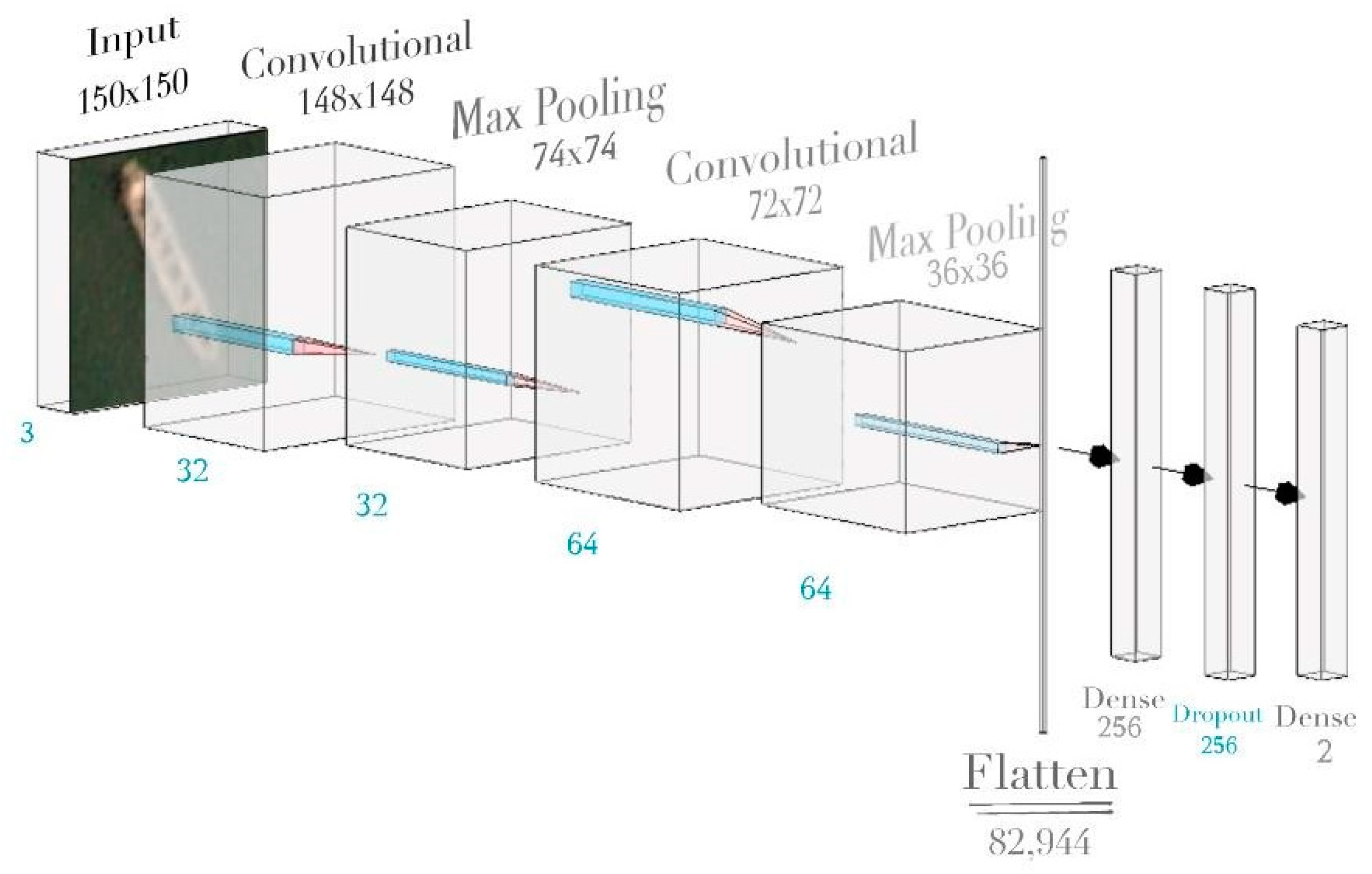
Figure 2.
(11, 11) Convolutional Layer Kernel Size Output.

Figure 3.
(3, 3) Convolutional Layer Kernel Size Output.
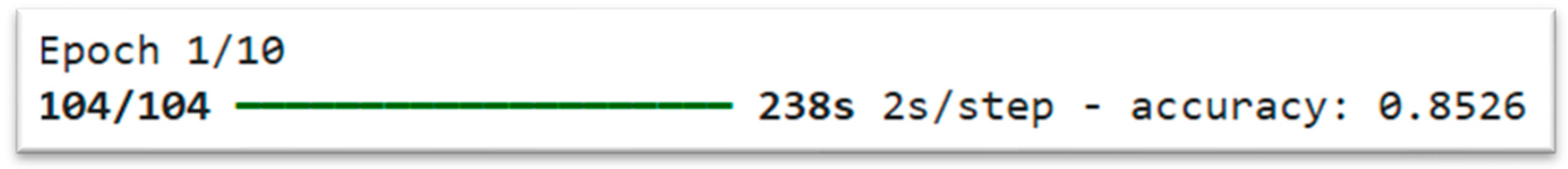
Figure 4.
Convoluted and Pooling Layers Code.
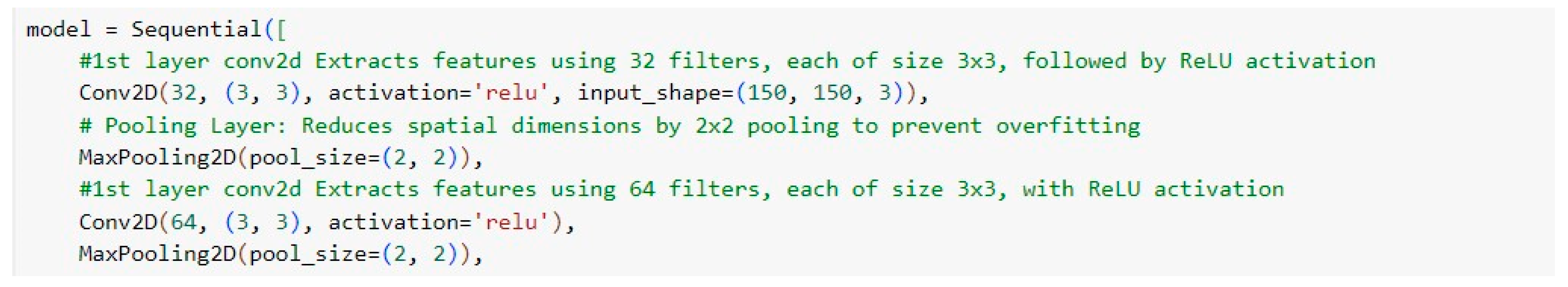
Figure 5.
Dropout and Dense Layers Code.
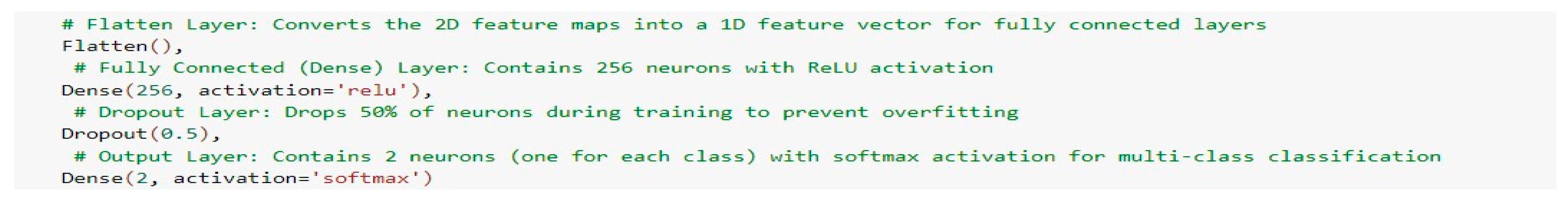
Figure 6.
Import Statements. Output Snippet: Upon executing, the environment confirms that Google Drive is mounted successfully, enabling smooth access to the dataset for subsequent processing.
Figure 6.
Import Statements. Output Snippet: Upon executing, the environment confirms that Google Drive is mounted successfully, enabling smooth access to the dataset for subsequent processing.
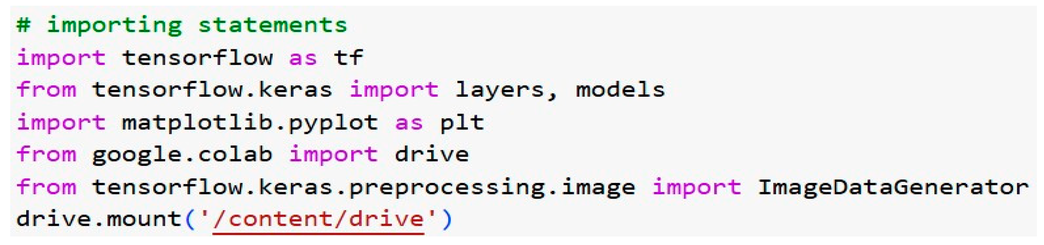
Figure 7.
Output Snippet: The visual output presents a set of 25 images, providing a clear overview of the dataset. Each image is labelled, assisting in the verification of data integrity and ensuring that augmentation techniques have been applied effectively.
Figure 7.
Output Snippet: The visual output presents a set of 25 images, providing a clear overview of the dataset. Each image is labelled, assisting in the verification of data integrity and ensuring that augmentation techniques have been applied effectively.
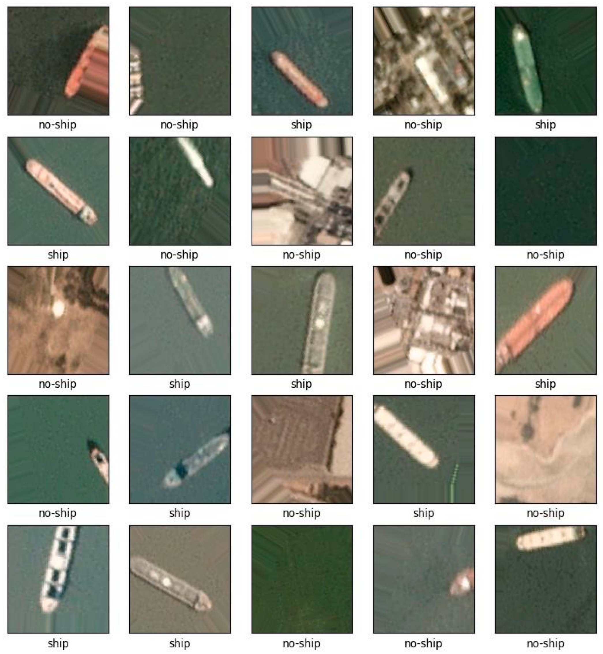
Figure 8.
Displays training and validation accuracy for each epoch, indicating the model’s learning progress over time.
Figure 8.
Displays training and validation accuracy for each epoch, indicating the model’s learning progress over time.
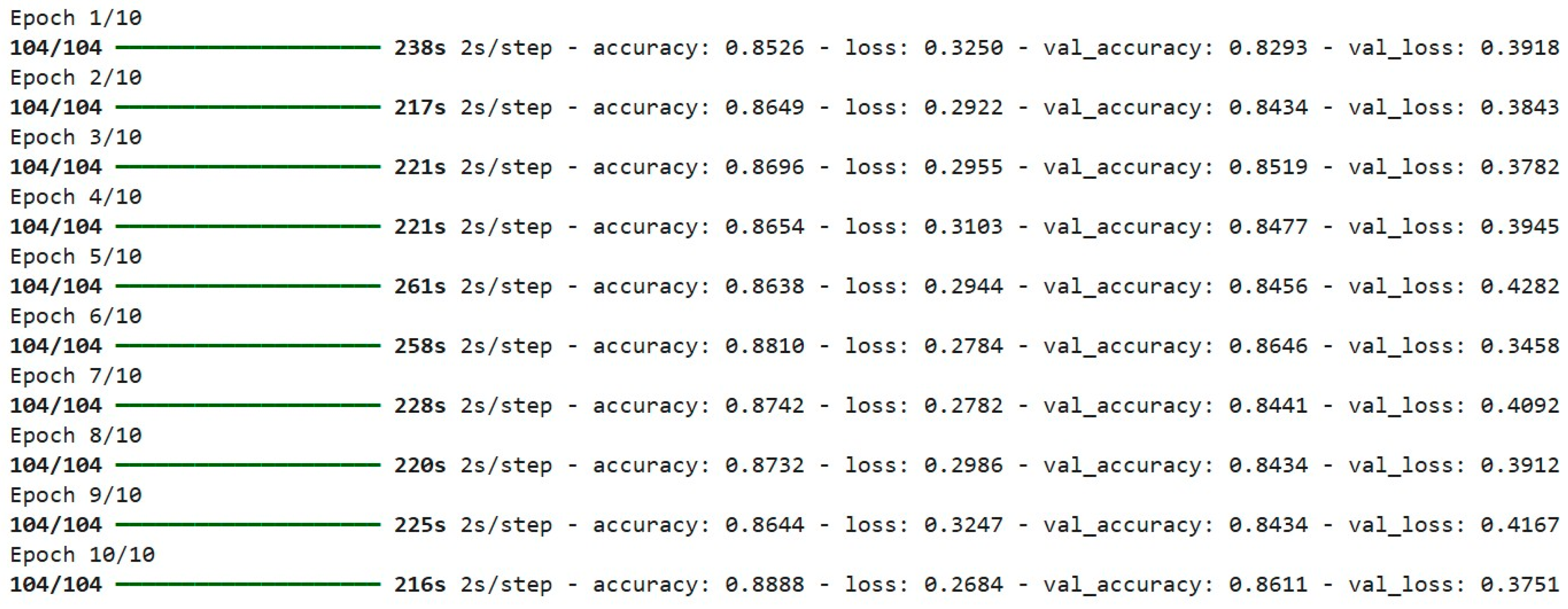
Figure 9.
Model Accuracy Output.
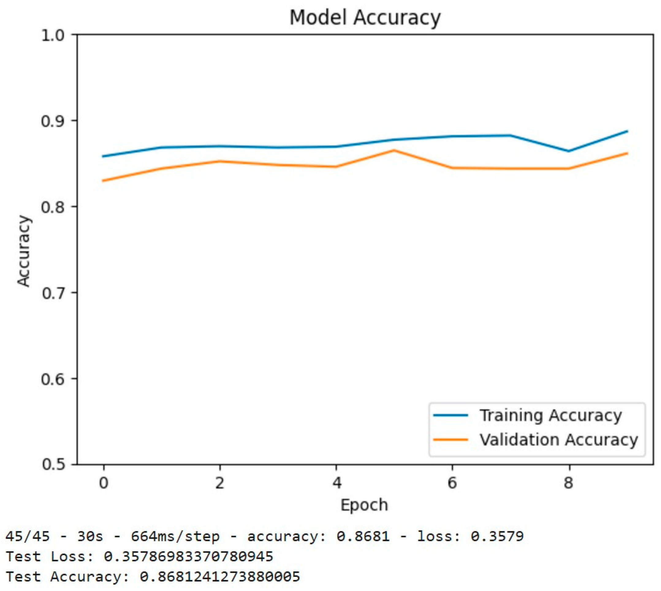
Figure 10.
Confusion Matrix and Classification Report Output.
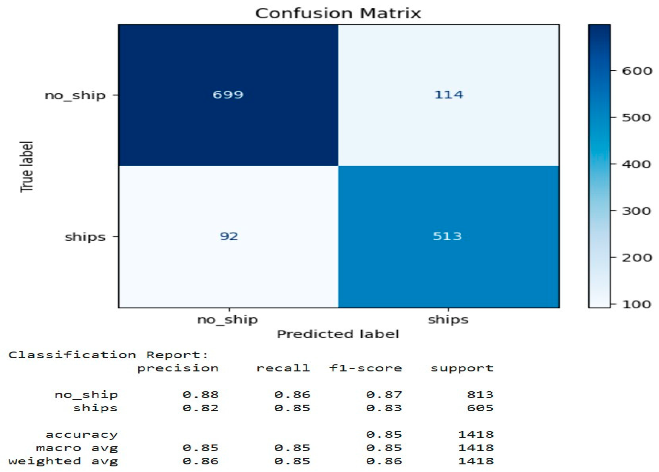
Figure 11.
Model Accuracy Evaluation.
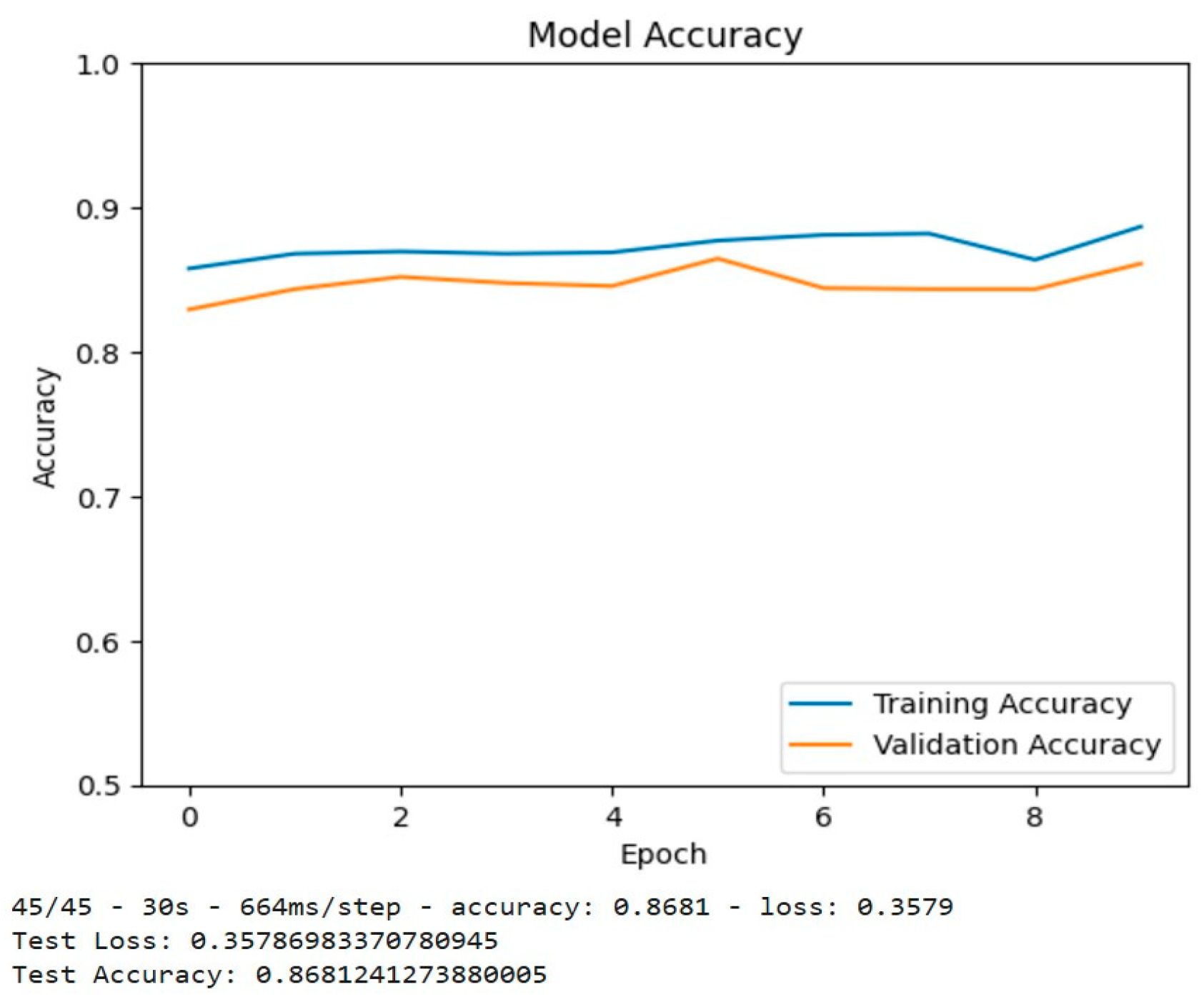
Figure 12.
Confusion Matrix and Classification Report.
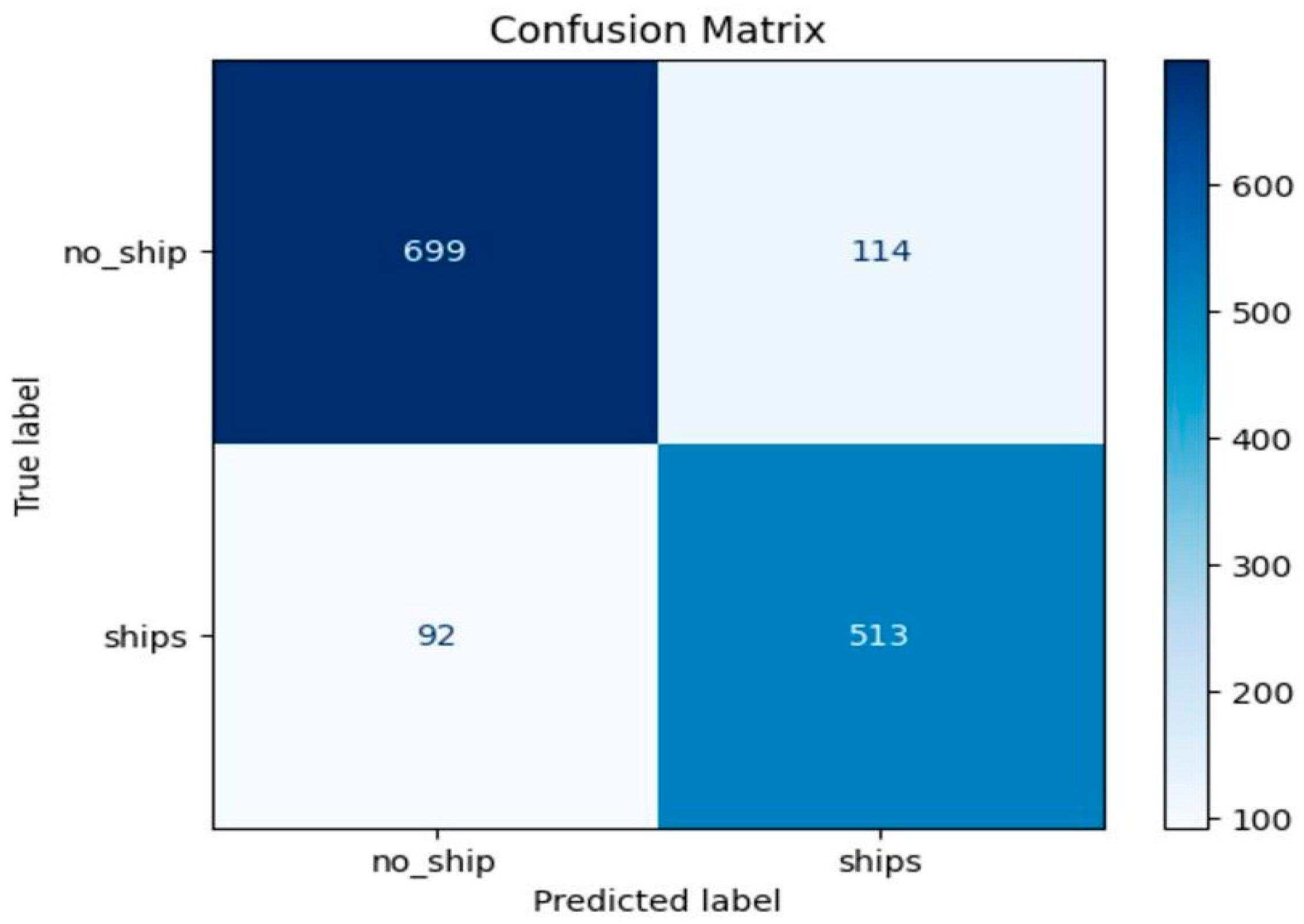
Figure 13.
Classification Report.
Disclaimer/Publisher’s Note: The statements, opinions and data contained in all publications are solely those of the individual author(s) and contributor(s) and not of MDPI and/or the editor(s). MDPI and/or the editor(s) disclaim responsibility for any injury to people or property resulting from any ideas, methods, instructions or products referred to in the content. |
© 2025 by the authors. Licensee MDPI, Basel, Switzerland. This article is an open access article distributed under the terms and conditions of the Creative Commons Attribution (CC BY) license (http://creativecommons.org/licenses/by/4.0/).
Copyright: This open access article is published under a Creative Commons CC BY 4.0 license, which permit the free download, distribution, and reuse, provided that the author and preprint are cited in any reuse.


