Submitted:
13 May 2024
Posted:
14 May 2024
You are already at the latest version
Abstract
The understanding of spatiotemporal variations in reference evapotranspiration (ETo) and its long-term trends is of paramount importance for water cycle studies, modeling, and water resource management, especially in the context of climate change. Therefore, the primary aim of this study is to critically evaluate the performance of various CMIP5 global climate models in simulating the Penman-Monteith reference evapotranspiration and its associated climate variables (maximum and minimum air temperature, incident solar radiation, relative humidity, and wind speed). This evaluation is based on data from nine climate models and 33 automatic meteorological stations (EMA) in the state of Mato Grosso, spanning the period 2007-2020. The statistical metrics used for evaluation include Bias, root mean square error, and Pearson and Spearman correlation coefficients. The projections of the most accurate model were then used to analyze the spatial and temporal changes and trends in ETo under the RCP 2.6, 4.5, and RCP 8.5 scenarios from 2007 to 2100. The HadGEM2-ES model projections indicate static averages similar to current conditions until the end of the century in the RCP 2.6 scenario. However, in the RCP 4.5 and 8.5 scenarios, there is a continuous increase in ETo, with the most significant increase occurring during the dry period (May to September). The areas of the Amazon biome in the north of Mato Grosso exhibit the largest increases in ETo when comparing the observed (2007-2020) and projected (2020-2100) averages. The trend analysis reveals significant changes in ETo and its variables across the state of Mato Grosso in the RCP 4.5 and 8.5 scenarios. In the RCP 2.6 scenario, significant trends in ETo are observed only in the northern Amazon areas. Despite not being observed in all AWSs, the trend analysis of the observed data demonstrates more intense changes in ETo and the existence of the evapotranspiration paradox with an increase in the Cerrado areas and reductions in the Pantanal and southern Amazon areas.
Keywords:
Penman-Monteith
; Global climate models
; RCP scenarios
; Mann-Kendall trend analysis
; Amazon
; Cerrado
1. Introduction
In recent decades, global climate change caused by anthropogenic factors has been observed in several regions of the planet, posing risks to ecosystems and human development [1,2,3]. Evidence of climate change includes increased global temperature, warming of the oceans, more extreme weather events, and changes in climate seasonality (Intergovernmental Panel on Climate Change [4]). Therefore, the ability to predict climate change is important to better understand its changes and impacts.
Assessing the impact of climate change on water resources is one of the main current challenges in hydrological studies [5] since the projection of water availability and demand allows the development of strategies to manage water use better. Water, especially in the context of providing subsidies for the design of irrigation and water distribution systems used in agriculture and urban supply [6,7]. Such projections, however, are highly dependent on evapotranspiration as they play a crucial role in determining plants' water needs [8], being an essential component in planning and scheduling irrigation and an important indicator of the functioning of water systems [9].
Different terms are used to describe evapotranspiration, with the Penman-Monteith method of "crop reference evapotranspiration (ETo)" being the one recommended by the Food and Agriculture Organization of the United Nations (FAO) in evapotranspiration estimates [10]. Evapotranspiration, however, is a complex parameter that controls the exchange of energy and mass between terrestrial ecosystems and the atmosphere and is governed by several climatic variables such as solar radiation, temperature, wind speed and atmospheric humidity [11,12]. Thus, since variation in any of these factors can affect the spatiotemporal distribution of evapotranspiration [13,14], performing spatiotemporal projections, as well as characterizing the trends of Evapotranspiration in the scenario of changes in these climate variables is of fundamental importance [15,16].
Global climate models (GCMs) are important tools for understanding and predicting the Earth's complex climate, as they consist of numerical models that represent the physical and chemical processes of the atmosphere and all its interactions with the other components of the Earth's system (hydrosphere, cryosphere, lithosphere and biogeochemical cycles) based on the use of basic equations, such as conservation of mass and energy, thermodynamics, hydrostatics and continuity [17,18]. The study and proposition of global climate models capable of projecting future climates are generally carried out by institutions and research groups that are part of the Intergovernmental Panel on Climate Change (IPCC) of the United Nations (UN); with around 40 GCMs from 20 research groups participating in the fifth phase of the Coupled Model Intercomparison Project Phase 5 CMIP5 [19], which present simulations of the future climate using different greenhouse gas emission scenarios, known as RCPs (Representation Concentration Pathway) scenarios.
However, despite the great availability of models, it is necessary to validate them for the region of interest to analyze how well these models can represent the current climate [20] and, thus, verify the reliability of their predictions. Furthermore, since climate change varies between different regions of the world, it is necessary to have studies on climate change for each region of interest.
The state of Mato Grosso, located in the Center-West region of Brazil, has a large territorial extension and insertion in the area of occurrence of the phytophysiognomies of the Pantanal Complex, savannah formations (Cerrado) and Amazonian formations, distributed in three distinct climatic types (Af - humid equatorial climate, Aw - tropical savannah climate, and Cwa - tropical climate) [21]. In addition to its great ecological diversity, the State stands out in agricultural production, being the largest grain producer in Brazil [22], although there is a lack of research focused on the variability and impacts of climate change on evapotranspiration [23,24].
Thus, the objective of this study was to evaluate the performance of different GCMs, find a simulation model that represents the current climatic conditions in the state of Mato Grosso, and subsequently evaluate whether future climate projections change the reference evapotranspiration (ETo) and its climatic variables in the state of Mato Grosso, Brazil.
2. Materials and Methods
2.1. Study Area and Data Acquisition
The study area comprises the state of Mato Grosso, Brazil, located between coordinates 06°00'S, 19°45'S and 50°06'W, 62°45'W. Climatically, according to Köppen's classification, the state is divided into a humid equatorial climate (Af), a tropical savanna climate (Aw) and a tropical high-altitude climate (Cwa), presenting two well-defined seasons: the rainy season (October to April) and the dry season (May to September) [21,25,26]. The state also has three biomes: the Amazon, the Cerrado, and the Pantanal.
The study used a monthly time series of data observed at automatic meteorological stations (AWSs) and data simulated by nine global climatological models (MCG) from Phase 5 of the Coupled Model Intercomparison Project (CMIP5). The observed time series were obtained from the AWSs of the National Institute of Meteorology (Inmet) located in 33 municipalities in Mato Grosso, Brazil (Figure 1).
The data simulated by the GCMs were obtained from the platform of the intergovernmental organization Copernicus Climate Change Service [27], encompassing data referring to the simulated periods from 2007 to 2100 in 3 climate scenarios (RCP 2.6, RCP 4.5 and RCP 8.5). Among the 40 CMIP5 GCMs, only those that presented the same minimum meteorological variables required in the evapotranspiration estimates available in the state's AWSs were selected. The description of the names, research groups of origin and spatial resolution of the CMIP5 models used in the study are presented in Table 1.
2.2. Reference Evapotranspiration (ETo) Estimates
Reference evapotranspiration estimates were obtained using the Penman-Monteith FAO (FAO-PM) equation using daily data on meteorological variables: incident global radiation (Hg - MJ m-2 day-1), relative air humidity (Rh - %), maximum air temperature (Tmax - °C), minimum air temperature (Tmin - °C) and average wind speed at 2.0 m of height (Ws - m s-1), according to Equation 1, with data from meteorological variables of the GCMs extracted from the pixel closest to the location of each AWS in the state. The FAO-PM method was chosen because it is the method recommended by the Food and Agriculture Organization of the United Nations (FAO) and combines physiological and meteorological parameters in estimating the ETo of a hypothetical grass surface with a height of 0.12 m, surface resistance of 70 s·m-1 and albedo of 0.23 [10].
where: ETo - is the reference evapotranspiration (mm day-1); SRD - is the net radiation at the surface of the crop (MJ m-2 day-1); G – is the heat flux density of the soil (MJ m-2 day-1); T - is the average air temperature at 2.0 m height (average value of Tmax and Tmin, °C); Ws - is the wind speed at 2.0 m height (m s-1); es - is the saturation vapor pressure (kPa); ea - is the current vapor pressure (kPa); Δ - is the slope of the saturation vapor pressure versus air temperature curve (kPa °C-1); γ - is the psychometric constant (kPa °C-1)
Detailed calculations of SRD, Δ and γ and other parameters necessary for computing ETo were obtained according to the procedure described in Allen et al. [10]. Furthermore, since the variable wind speed in the state's AWSs and MCGs is obtained at 10.0 meters, the average speed at 2 meters was obtained according to Equation 2.
where: SW2 - is the wind speed at 2 meters (m s-1); SW10 - is the wind speed at 10 meters (m s-1); H - is the height at which the wind speed was obtained (m) – 10.0 meters;
2.3. Assessment of Estimation Errors and Choice of GCM
The accuracy of the estimates of the nine GCMs was evaluated by comparing the simulated data from ETo and its meteorological variables between the years 2007 and 2020 with the data observed in the AWSs of Mato Grosso. Estimation errors were measured using Bias measures (Equation 3), root mean square error (RMSE - Equation 4), normalized RMSE (Equation 5), Pearson's correlation coefficients (rohp - Equation 6) and Spearman (rohs -Equation 7). Finally, the models were ranked to receive the best positions (lowest value of weighted errors) for the GCM, whose bias and RMSE results were closest to zero and whose correlation coefficient, in absolute values, was close to one.
where: Pi - estimated data; Oi - observed data; "Ō"- average of the observed data; "" - average of the estimated data; N – number of sample values; d - order difference between the simulated and observed values.
2.4. Spatiotemporal Analysis and Average Test of Reference Evapotranspiration Projections
The projections of the best GCM were then evaluated through graphical comparisons of the annual and seasonal spatiotemporal variations of the three RCP scenarios (Optimistic scenario - RCP 2.6, Average scenario - RCP 4.5, and Pessimistic scenario - RCP 8.5) with the conditions observed in the AWSs of Mato Grosso. Furthermore, the statistical mean differences of the simulated ETo in the four projection periods (current – 2007 to 2020, short – 2021 to 2050, medium – 2051-2075 and long – 2076-2100) of the three scenarios were compared with each other and between the mean observed in AWSs using the non-parametric Kruskal-Wallis test (α=0.10), with differences expressed using the Wilcoxon-Mann-Whitney test.
2.5. Trend Analysis and Sen’s Test
The Mann-Kendall test [28,29] was used to detect the existence of annual trends in ETo and its meteorological variables in the simulated period of 2007-2100 in the three scenarios (RCP 2.6, RCP 4.5 and RCP8.5) and in the period of data observed in the AWSs (2007-2020). Since the Mann-Kendall test requires a complete data series, gaps in the observed meteorological data were filled by the simple linear regression method using the GapMET software, as Sabino and Souza [30] recommended. The Mann-Kendall test is based on two hypotheses: the null hypothesis (H0), which assumes that the series is stationary (no trend), and the alternative hypothesis (H1), which indicates the existence of a trend. The significance level used in this study to reject H0 was 0.10. Furthermore, the Mann-Kendall test allows you to check the direction of the trend (positive or negative) using the sign (+ or -) associated with the Z value of the test.
Finally, the amplitude of the trends was measured using Sen’s robust linear regression [31]. Sen’s test is a non-parametric slope estimator based on the median and is recommended for being robust against outliers and widely used in estimating trends in evapotranspiration and climate variables [32,33].
3. Results and Discussion
3.1. Choice of Climate Projection Models
The average relative errors for the performance metrics of the nine global climate models (GCMs) in estimating the meteorological variables incident solar radiation (Rs), maximum temperature (Tmax), minimum temperature (Tmin), relative humidity (RH) and wind speed (VV) are presented in Figure 8. Although each GCM exhibits mixed performance results for the different metrics in each variable, comparing weighted errors demonstrates that the three models with the most accurate estimates were CESM1-CAM5, CNRM-CM5 and HadGEM2 -ES. These three GCMs also stood out due to the absolute bias and RMSE-Normalized values below 0.1 in the estimates of the SRD, Rh and SW variables.
Figure 2.
Average bias performance metrics, normalized root mean square (Normalized RMSE), Spearman correlation coefficient (rohs) and weighted error of the 9 GCMs in estimating the meteorological variables net radiation (SRD), maximum temperature (Tmax), minimum temperature (Tmin), relative humidity (RH) and wind speed (SW) obtained in the locations of the 33 AWSs in the state of Mato Grosso, Brazil.
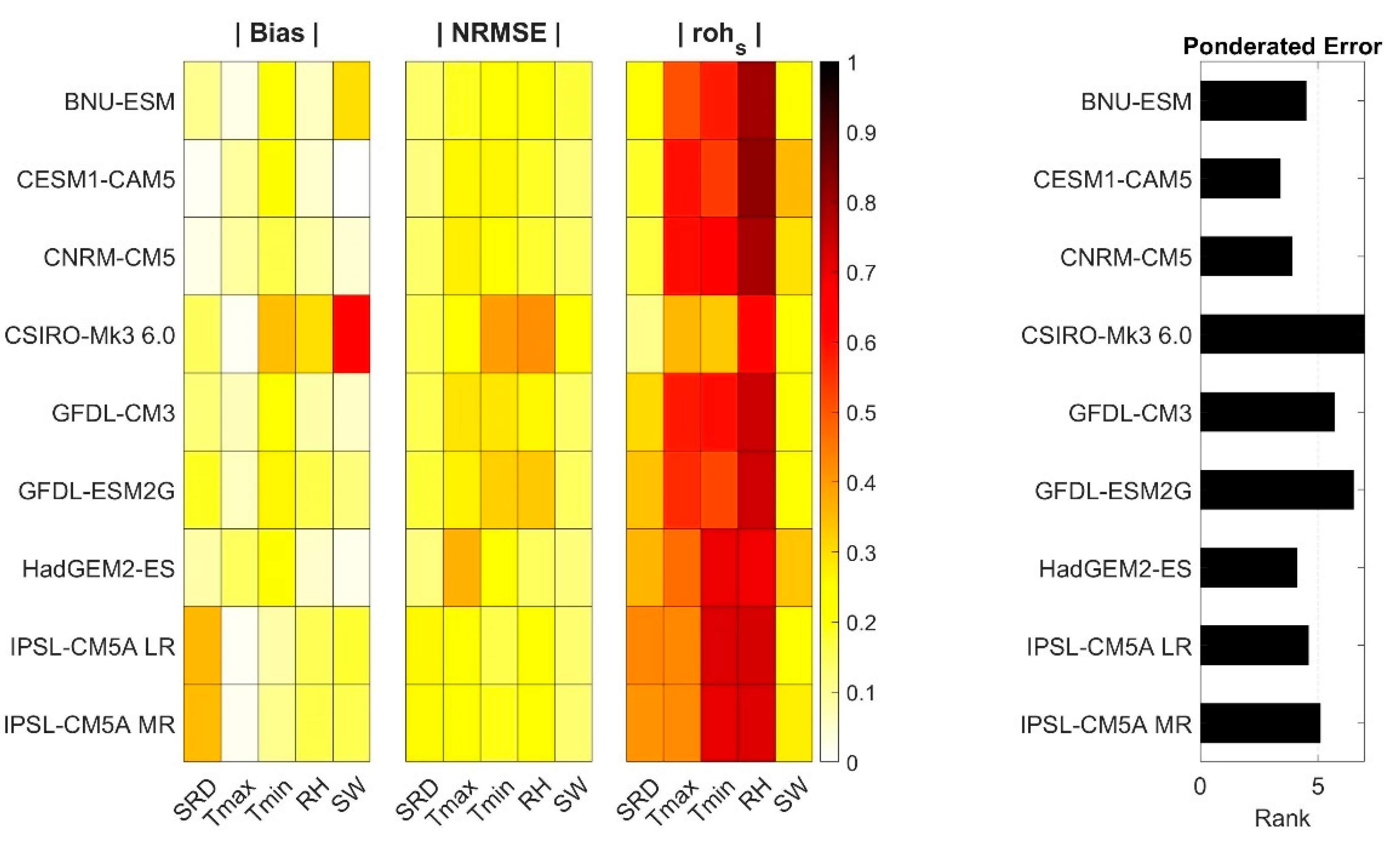
Although all models presented good correlation results with the observed data of RH, Tmax and Tmin (in general, greater than 0.6), the variables SRD and SW presented low correlations (less than 0.45) being the best correlation results for incident solar radiation obtained by the IPSL-XM5A LR, IPSL-XM5A MR and HadGEM2-ES models, and the best results for wind speed were observed in the CESM1-CAM5, HadGEM2-ES and CNRM-CM5 models. However, although there is a good correlation between the IPSL-XM5A LR and IPSL-XM5A MR models with the observed data of the SRD variable, these presented, on average, the largest bias errors found for net radiation (35% bias).
The CSIRO-Mk3 6.0, GFDL-ESM2G, and GFDL-CM3 models presented the lowest performances in estimating meteorological variables, highlighting the CSIRO-Mk3 model, whose bias error varied from 0.3 to 0.6 for the Tmin, RH and SW variables, and maximum correlation of 0.6 (found in the relative humidity variable).
The distribution of the performance metrics of the nine MCGs in the reference evapotranspiration estimates calculated in the 33 AWSs of Mato Grosso are presented in the Boxplot of Figure 3. Again, the best results are found in the MCGs CESM1-CAM5, CNRM-CM5 and HadGEM2-ES (|bias| < 20%, RMSE < 0.4 and 0.3< rohp >0.7), while the MCGs IPSL-XM5A LR, IPSL-XM5A MR in addition to higher error averages showed a greater dispersion of metrics (10% < |bias| < 60%, 0.3 > RMSE < 0.8 and 0.05< rohp >0.85). The good performance of the HadGEM2-ES model estimates also stands out due to the low dispersion of the metrics estimated in the 33 stations in the state, demonstrating that the model can estimate ETo in the different environmental and climatic conditions of Mato Grosso.
These results agree with those found in the literature for the South American region, in which most of the CMIP5 models were capable of satisfactorily simulating the variables linked to evapotranspiration, with different performances depending on the climate variable being analyzed, as well as the indication of the best model, considering only one climate variable or the set of variables analyzed concomitantly, can be composed of different GCMs depending on the region of interest [34,35,36]. Despite this, the use of the HadGEM2-ES model is still considered capable of simulating ETo cycles quite skillfully, according to a study carried out by Guimarães et al. [36] in the northeast region of Brazil, as well as in studies of the Martins and Silva [35], Silva et al. [37], Rocha et al. [38] and Gomes et al. [39] in the Amazon basin.
In general, the two models with the best results for estimating ETo in Mato Grosso in the current period (2007-2020) were CESM1-CAM5 and HadGEM2-ES. However, since the HadGEM2-ES model presented less dispersion of ETo estimation errors, as well as better performance in estimating the variables SRD, RH and SW, these variables have a greater impact on ETo estimates using the method of Penman-Monteith for the region [40]; in the following stages of this research, the MCG HadGEM2-ES will be the model used in the evaluations of ETo projections.
3.2. Reference Evapotranspiration Climate Projections (ETo)
The annual means and standard deviation of the reference evapotranspiration estimates and their meteorological variables projected by HadGEM2-ES in the RCP 2.6, 4.5 and 8.5 scenarios between the years 2007 and 2100 in the AWSs of the state of Mato Grosso are presented in Figure 4. Note It is clear that until the middle of the 21st century, ETo estimates are similar between the three scenarios. Furthermore, ETo in the RCP 2.6 scenario remains close to the current average (3.9 ± 0.8 mm day-1) until 2100, while in RCP 8.5, there is an increase in ETo after 2050, reaching 5.2 ± 1.3 mm day-1 in 2100.
These visual results are confirmed by the Kruskal-Wallis test (Table 2), which demonstrates that significant differences (α = 0.10) between the averages estimated in the three projections only occur from the period 2050-2075 when the annual average of ETo in the RCP 8.5 scenario (4.42 mm day-1) becomes statistically greater than that projected by the RCP 2.6 scenario (4.13 mm day-1). This differentiation between the projected scenarios continues to increase in subsequent years, reaching statistically different averages of ETo between the three RCPs between 2076-2100.
The evaluation of the differences within each scenario demonstrates that the RCP 4.5 and 8.5 projections continuously increase ETo, with significant differences to the current condition (2007-2020) from 2050 onwards. The RCP 2.6 scenario, however, despite presenting a significant increase until the period between 2050 and 2075, shows a reduction in the average ETo to values similar to the current one (2007-2020) in the last quarter of the 21st century.
Regarding the differences between the annual averages of the scenarios in the different periods evaluated and the annual averages observed in the AWSs, it is concluded that the projections of the RCP 2.6 scenario between 2007 and 2100 do not differ from the data observed in the state of Mato Grosso, while the scenarios RCP 8.5 and RCP 4.5 at ETo show a significant increase from the period 2050-2075 and 2075-2100, respectively.
The increase in ETo from 2050 onwards in RCP 4.5 and 8.5 projections is, in general, justified due to the gradual and continuous increase in air temperature values since the RCP 2.6 scenario presents temperature stabilization and consequent stagnation of ETo averages in the mid-21st century (Figure 4) [36,39]. However, changes in other meteorological variables have important contributions to changes in evapotranspiration since ETo estimates using the PM method in the state are more sensitive to changes in RH and WS than to temperature [40]. Thus, the distinction between the ETo averages estimated in RCPs 4.5 and 8.5 is mainly due to the reduction in relative humidity and increase in wind speed (Figure 4), which occur more significantly in RCPs 8.5, enabling the scenario pessimism to become statically different from the current conditions observed already between the years 2050-2075 (Table 2).
Similar results are found in the literature for other regions of Brazil, in which the ETo averages in the RCP 4.5 and RCP 8.5 scenarios become statically different from the middle of the century onwards [36,39]. However, the statistical differences between observed and projected data were identified only from 2050 onwards. They may, in part, have occurred due to the decision to divide the sub-periods evaluated into approximately 25 years since Gomes et al. [39], when evaluating smaller sub-periods, found significant differences between the ETo estimated in the RCP 8.5 scenario and the current conditions, from the 2028-2038 time interval.
The variations in the monthly averages of reference evapotranspiration in the RCPs 2.6, 4.5 and 8.5 scenarios in the four periods evaluated (Figure 5) demonstrate that the increase in ETo estimates is more significant in the dry months in the state of Mato Grosso, mainly between July to October. Even in the RCP 2.6 scenario, in which annual averages remain similar throughout the century, it is possible to observe an increase of up to 0.50 mm day-1 in the monthly averages for September when comparing 2007-2020 and 2075 -2100.
When evaluating the pessimistic scenario (RCP 8.5), the increase in ETo during the dry period (May-September) could reach 1.5 mm day-1 by the end of the century, totaling an average ETo of 5.2 ± 1.2 mm day-1. The increase in evapotranspiration in the RCP 8.5 scenario is noticeable even during the rainy season (October-April), reaching, on average, 4.8 ± 0.6 mm day-1 in the period 2075-2100, which represents an increase of up to 0.4 mm day-1 compared to current averages.
However, it is important to highlight that the increase in ETo may be even more pronounced because, as discussed previously, the HadGEM2-ES MCG presents an uncorrected underestimation bias with a root mean square error (RMSE) of approximately 0.2 mm day-1 in Mato Grosso. The monthly averages of reference evapotranspiration observed in the state's AWSs between 2007-2020 and estimated by the MCG HadGEM2-ES in the three scenarios between the years 2007-2100, as well as the difference between the averages estimated and observed by the MCG are presented in Figure 6 and Figure 7, respectively. In addition to the increase in ETo, the projected changes in the state's climate still imply changes in the seasonal behavior of ETo.
It is noted that under current conditions, the minimum ETo values occur between April and July (with a minimum in June), while the maximum values occur between August and October (with a maximum in September). However, in RCP 4.5 and 8.5 scenarios, there is a reduction in the number of months with minimum ETo and an increase in months with maximum ETo. This condition is more explicit in the RCP 8.5 scenario from 2075 onwards, when ETo starts to present similar averages between January and July (4.3 ± 0.4 mm day-1), followed by a rapid increase in ETo between August and December, reaching maximums of up to 6.6 ± 0.5 mm day-1 in the months of September-October.
The changes in the seasonality of reference evapotranspiration are consistent with recent literature, which demonstrates significant changes in the seasonal behavior of ETo, mainly after 2050 [36,39]. Such changes demonstrate an average increase in annual ETo associated with a more significant increase in ETo during the dry period [39,41,42], implying, in general, that the regions that already have an inconsistent water supply due to high seasonal variation in precipitation may experience even more inconsistent water balances due to increased evapotranspiration demand in dry periods [43].
The changes in seasonality with a greater increase during the end of the dry period and the beginning of the rainy season, as previously mentioned, may be mainly linked to reductions in relative air humidity and an increase in wind speed [43,44], since, according to Greve and Seneviratne [45], tropical regions and their transition areas in South America may present trends in the future towards intensification of arid environmental conditions characterized by low relative humidity, higher wind speed and high evapotranspiration rates. Furthermore, net radiation, despite not varying as significantly as the other variables (Figure 4), must be taken into account as one of the factors since previous studies have indicated this component as one of the main variables affecting the seasonality of ETo in the Amazon region [9,40,46].
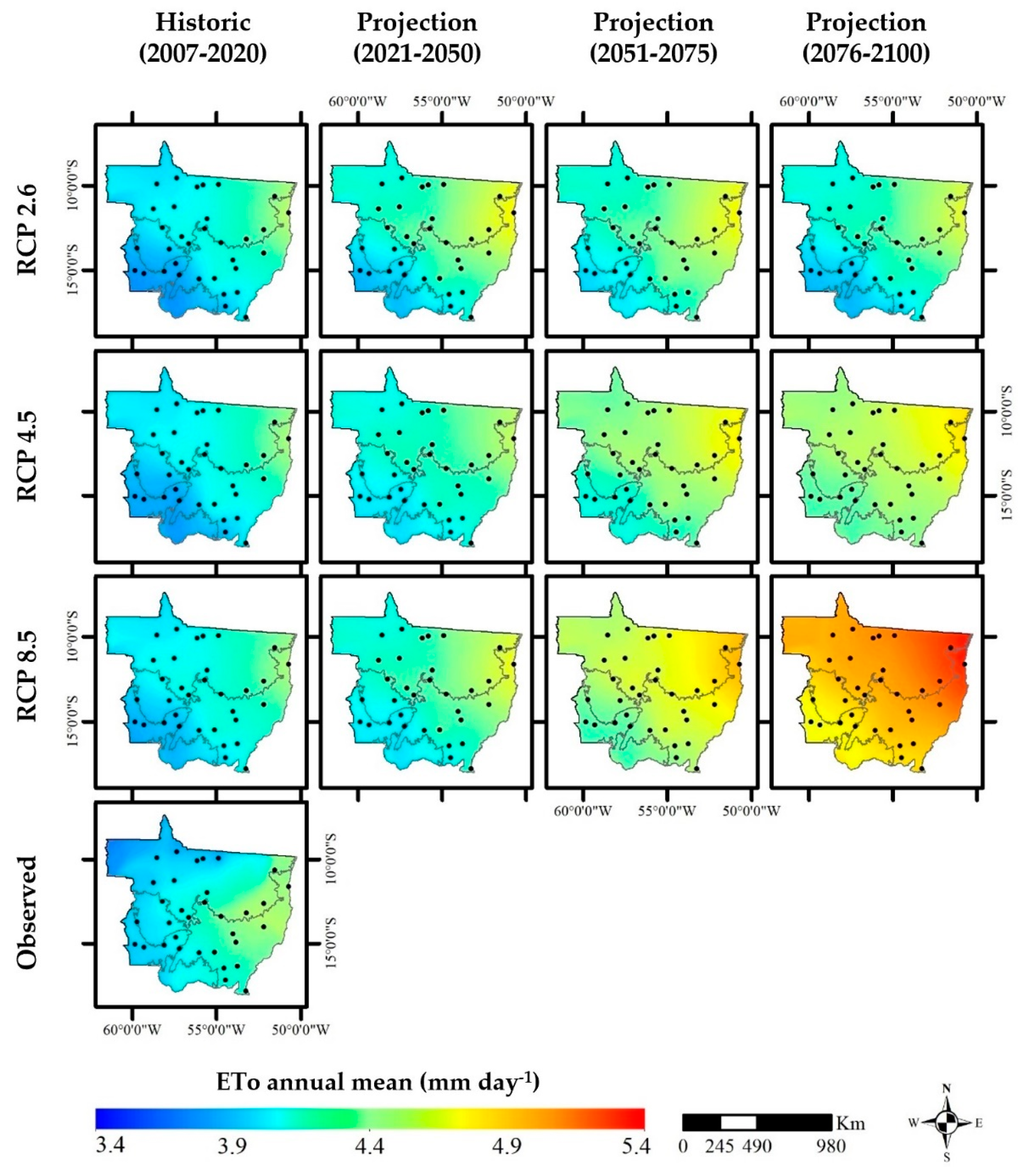
Figure 8 and Figure 9 present the spatial distribution of reference evapotranspiration averages observed in the AWSs of the state of Mato Grosso from 2007 to 2020 and the averages estimated by the HadGEM2-ES model in the three climate scenarios (RCP 2.6, RCP 4.5 and RCP 8.5) and four periods evaluated (2007-2020, 2021-2050, 2051-2075 and 2076-2100), respectively. The differences between the averages observed in the EMA and estimated by the model are presented in Figure 8 and Figure 9, respectively.
Figure 8.
Interpolated spatial distribution of reference evapotranspiration (ETo) annual average observed in the AWSs of the state of Mato Grosso, between the years 2007 and 2020, and estimates by the HadGEM2-ES model in the RCPs scenarios (2.6, 4.5 and 8.5) in different periods of the 21st century. XXI century. NOTE: Lines on the map demarcate the biomes and point to the AWSs in the state of Mato Grosso.
In the estimates for the current period (2007-2020), it is observed that HadGEM2-ES presents a different bias depending on the biomes in the state of Mato Grosso. In the Amazon region, north of the state, there is an overestimation of up to 0.2 mm day-1 in all scenarios. In contrast, in the other areas of the state (Cerrado and Pantanal), there is an underestimation of ETo of up to 0.3 mm day-1 (Figure 8 and Figure 9), highlighting the higher altitude areas south of Mato Grosso.
In the model projection estimates for the period between 2007-2100, the RCP 2.6 scenario, as discussed previously, is the only one that maintains similar ETo values throughout the century in all areas of the state, presenting, however, a peak in evapotranspiration between the years 2050-2075 (Figure 8). It is noted, however, that the ETo estimates in the RCP 2.6 scenario during the peak period (2050-2075) are the closest to the averages observed in the AWSs of the state of MT in the current period (2007-2020) (Figure 9). In the projections of the RCP 4.5 and 8.5 scenarios, an increase in ETo is observed throughout the state, reaching average annual evapotranspiration ranging from 4.3 to 4.8 mm day-1 in the last quarter of the century in the RCP 4.5 scenarios, as well as 4.7 to 5.4 mm day-1 in the pessimistic scenario (RCP 8.5) (Figure 9).
In all scenarios, the highest reference evapotranspiration rates occur in the Cerrado areas of the state, mainly in the Cerrado Setentrional region (northeast region of the Cerrado of Mato Grosso), as well as the lowest estimates are distributed in areas close to the Pantanal and the southern portion of the Amazon, both in the southwest region of the state. However, when comparing the data observed in the AWSs of Mato Grosso with the scenario estimates, it is noted that the greatest change in the evapotranspiration rate occurs in the northern Amazon region, where ETo can have an average annual increase of up to 1. 3 mm day-1 (RCP 8.5), while in the Cerrado the increase is approximately 0.7 mm day-1 (RCP 8.5) (Figure 9).
3.3. Trends Analysis
The evaluation of the behavior of the annual trends of the observed and simulated averages of ETo and its meteorological variables in the state of Mato Grosso are presented in Table 5. Regarding the analysis of the averages of the data simulated by the HadGEM2-ES model in the long term (2007-2100), it is observed that in the RCP 4.5 and 8.5 scenarios, all variables showed significant trends, while in the RCP 2.6 scenario, significant trends were identified only in the variables Tmax, Tmin and SW. These results agree with those discussed previously regarding reference evapotranspiration projections, making it possible to observe, until the end of the century, stationary behavior of ETo in the RCP 2.6 scenario, as well as a tendency for ETo to increase by 0.05 and 0.12 mm day-1 decade-1 in RCP 4.5 and 8.5 scenarios, respectively.
The increase in ETo in RCP 4.5 and 8.5 scenarios is justified due to changes in the averages of their meteorological variables, such as increases in incident solar radiation, wind speed and maximum and minimum temperatures, and reductions in average relative humidity. Likewise, the stationarity of ETo in the RCP 2.6 scenario can be explained by the fact that incident solar radiation, the main variable influencing evapotranspiration estimated by the Penman-Monteith method in the state, did not show a significant trend, moreover, despite being possible to observe increasing trends in the variables wind speed and maximum and minimum temperature, the changes were not sufficient to influence the ETo averages, as they are variables with a lower degree of global sensitivity for the Penman-Monteith method [40] and whose degree of inclination of the trend lines is considered low, with an increase up to 2100 of approximately 0.04 m s-1 (SW), 0.64 °C (Tmax), and 0.46 °C (Tmin).
Regarding the results of the trend analysis of data observed in the AWSs of Mato Grosso between the years 2007 and 2020, the existence of significant trends in reference evapotranspiration was not verified, with the only variables with significant trends being the maximum air temperature (+0.567 °C decade-1) and wind speed (-0.111 m s-1 decade-1). However, these results must be evaluated with reservations due to the database containing a few years (2007-2020), which can lead to errors in trend analysis since the time series can contain climate anomalies caused by both short-term events such as the Southern Oscillation phenomenon (ENSO or El Niño), whose variation can occur over periods of 2 to 10 years [47], as well as long-term events such as the Pacific Decadal Oscillation (PDO), whose oscillation pattern can last 20 to 30 years [48]. The problem regarding the amount of data needed for trend analysis is even more explicit when considering the trends in data simulated by the HadGEM2-ES model in the same data period (2007-2020) in which the occurrence of significant trends does not match with the results obtained with the long-term database (2007-2100).
However, despite the reservations, some important points can be raised regarding the trends observed in the data collected in the AWSs of Mato Grosso, especially when evaluating the AWSs individually (Figure 10), as is the case, for example, of the concentration of significant trends in certain biomes, as well as the intensity of the trends (degree of inclination of Sen's straight line) found in the observed data being, in general, greater than that of the data simulated by the HadGEM2-ES model in the short and long term.
Initially, we can notice that in the data simulated by HadGEM2-ES, all AWSs in the state show significant trends towards an increase in ETo in the RCP 4.5 and RCP 8.5 scenarios, as well as the AWSs in the northern Amazon region in the RCP 2.6 scenario, while, in the observed data the occurrence of significant trends was concentrated in the Northern Cerrado region and areas of the southern Amazon. Furthermore, the trends in the simulated data represent a maximum variation in ETo increment between 0.02 mm day-1 decade-1 (RCP 2.6) and 0.14 mm day-1 decade-1 (RCP 8.5). In contrast, in the analysis from the data observed in the AWSs of the Northern Cerrado region, for example, there are trends towards a more significant increase in ETo (significant trends of increase of 0.27 and 0.51 mm day-1 decade-1). On the other hand, in the region close to the Pantanal, in the south of the Amazon biome, contrary to the simulated data, the analysis of the observed data demonstrated trends of reduction in ETo (-0.36 mm day-1 decade-1), which are associated with reductions in incident radiation and wind speed in the region.
Similar results that show an increase in evapotranspiration due to global climate change, both in observed and simulated data, have been published in the literature in recent years [49,50,51,52,53,54,55], with the increase in temperature and the greater amount of available energy being the main cause of the increase in evapotranspiration [51]. On the other hand, the decrease in evapotranspiration, as noted in the observed data, has also been reported in certain climatic regions of the world, such as in dry and humid climates in the United States [56,57], in tropical and subtropical climates in China [51,58,59], in semi-arid climate in Turkey [60,61,62,63] and in arid climate in Iran [64], this phenomenon being known as the "evaporation paradox" [51,62].
The "evaporation paradox" represents a situation in which a decrease in evapotranspiration accompanies global warming [63], which can be explained by the decrease in solar radiation, following the increase in cloud cover and the concentration of aerosols and pollutants in the atmosphere [56,62,66], as well as an increase in relative humidity [67] and a reduction in wind speed [66]. Thus, the tendency to reduce ETo in the southern Amazon and Pantanal regions can be explained by reductions in incident radiation and wind speed (Figure 10), probably caused by changes in concentrations and types of aerosols due to biomass burning as observed in the papers of Palácios et al. [68,69,70] who demonstrate that the occurrence of fires in the Amazon and Pantanal areas of Mato Grosso are directly linked to the scattering of solar radiation and consequently to energy balances.
4. Conclusions
The global climate models with the best performance in estimating the Penman-Monteith reference evapotranspiration in the state of Mato Grosso were CESM1-CAM5 and HadGEM2-ES, with the HadGEM2-ES model being the one indicated for evaluating ETo projections as it presents lower dispersion of estimation errors, as well as better estimates of the variables incident solar radiation, relative humidity and wind speed, with |bias| < 20%, normalized RMSE < 0.4 and correlation coefficient between 0.3 and 0.7.
The analysis of the projections of the HadGEM2-ES model demonstrates static averages similar to the current conditions until the end of the 21st century in the RCP 2.6 scenario. In contrast, in the RCP 4.5 and 8.5 scenarios, ETo continuously increases, with significant differences from the current condition from 2050.
All climate scenarios (RCPs) of the HadGEM2-ES model indicate changes in the seasonality of evapotranspiration in the state of Mato Grosso until 2100. This includes an increase in the period with higher ETo values and a more significant increase in ETo averages in the dry months, mainly between July and October.
The spatial distribution of ETo in all projected scenarios remains similar to those currently observed, with higher averages in the Cerrado areas and lower ones in the Amazon and Pantanal areas. However, the areas of the Amazon biome, mainly in the north of Mato Grosso, show the largest increases when comparing the averages observed in the current period and projections between 2020 and 2100.
The trend analysis of data from the HadGEM2-ES model shows significant changes in evapotranspiration and its variables in all locations evaluated until the end of the century in RCP 4.5 and 8.5 scenarios. In the RCP 2.6 scenario, despite a significant trend in ETo being limited to areas in the northern Amazon, increases in the variable wind speed and maximum and minimum temperatures are observed in most areas of the state of Mato Grosso.
The trend analysis of data observed in the AWSs in Mato Grosso between 2007 and 2020 demonstrates that although not all AWSs present significant results with ETo trends, these are more intense. Furthermore, the state has an evapotranspiration paradox in which there is an increase in evapotranspiration in the Cerrado areas and reductions in the Pantanal and southern Amazon areas.
Author Contributions
Conceptualization, M.S and A.P.S.; Methodology, M.S., F.T.A. and A.P.S.; Software, M.S.; Validation, M.S.; Formal analysis, M.S. and A.P.S.; Investigation, M.S.; A.C.S., F.T.A. and A.P.S.; Resources, A.P.S.; Data curation, M.S. and A.P.S.; writing—original draft preparation, M.S.; writing - review and editing, M.S., A.C.S., F.T.A. and A.P.S.; Visualization, A.C.S., F.T.A. and A.P.S.; Supervision, A.C.S. and A.P.S.; Project administration, A.P.S.; funding acquisition, F.T.A. and A.P.S. All authors have read and agreed to the published version of the manuscript.
Funding
This research was funded by Coordenação de Aperfeiçoamento de Pessoal de Nível Superior – Brazil (CAPES) – Finance Code 001; The National Council for Scientific and Technological Development (CNPq) - Process 308784/2019-7; and, the Foundation for Research Support of Mato Grosso State (FAPEMAT) - Research Project Process 0182944/2017.
Data Availability Statement
The automatic weather stations (AWSs) data used in this study can be accessed by the Instituto Nacional de Meteorologia (INMET) databank website: https://bdmep.inmet.gov.br/# (accessed on 13 May 2024).
Acknowledgments
We thank the Federal University of Mato Grosso, specifically the Postgraduate Program in Environmental Physics.
Conflicts of Interest
The authors declare no conflicts of interest.
Appendix A

Table A1.
INMET automatic weather stations (AWS) in the Mato Grosso, Brazil.
| AWS | AWS name | Biome | Latitude (°) | Longitude (°) | Altitude (m) |
|---|---|---|---|---|---|
| A-901 | Cuiabá | Cerrado | -15.56 | -56.06 | 242 |
| A-902 | Tangará da Serra | Amazon | -14.65 | -57.43 | 440 |
| A-903 | São José do Rio Claro | Cerrado- Amazon | -13.45 | -56.68 | 340 |
| A-904 | Sorriso | Cerrado- Amazon | -12.56 | -55.72 | 379 |
| A-905 | Campo Novo do Parecis | Cerrado | -13.79 | -57.84 | 525 |
| A-906 | Guarantã do Norte | Amazon | -9.95 | -54.90 | 284 |
| A-907 | Rondonópolis | Cerrado | -16.46 | -54.58 | 290 |
| A-908 | Água Boa | Cerrado | -14.02 | -52.21 | 440 |
| A-910 | Apiacás | Amazon | -9.56 | -57.39 | 218 |
| A-912 | Campo Verde | Cerrado | -15.53 | -55.14 | 748 |
| A-913 | Comodoro | Cerrado | -13.71 | -59.76 | 577 |
| A-914 | Juara | Amazon | -11.28 | -57.53 | 263 |
| A-915 | Paranatinga | Cerrado | -14.42 | -54.04 | 477 |
| A-916 | Querência | Amazon | -12.63 | -52.22 | 361 |
| A-917 | Sinop | Cerrado- Amazon | -11.98 | -55.57 | 367 |
| A-918 | Confresa | Cerrado- Amazon | -10.64 | -51.57 | 233 |
| A-919 | Cotriguaçu | Amazon | -9.91 | -58.57 | 265 |
| A-920 | Juína | Amazon | -11.38 | -58.77 | 365 |
| A-921 | São Felix do Araguaia | Cerrado | -11.62 | -50.73 | 201 |
| A-922 | Vila Bela da Santíssima Trindade | Amazon | -15.06 | -59.87 | 213 |
| A-924 | Alta Floresta | Amazon | -10.08 | -56.18 | 292 |
| A-926 | Carlinda | Amazon | -9.97 | -55.83 | 294 |
| A-927 | Brasnorte (Novo Mundo) | Cerrado- Amazon | -12.52 | -58.23 | 426 |
| A-928 | Nova Maringá | Cerrado- Amazon | -13.04 | -57.09 | 334 |
| A-929 | Nova Ubiratã | Cerrado- Amazon | -13.41 | -54.75 | 466 |
| A-930 | Gaúcha do Norte | Cerrado- Amazon | -13.18 | -53.26 | 376 |
| A-931 | Santo Antônio do Leste | Cerrado | -14.93 | -53.88 | 664 |
| A-932 | Guiratinga | Cerrado | -16.34 | -53.77 | 525 |
| A-933 | Itiquira | Cerrado | -17.17 | -54.50 | 593 |
| A-934 | Alto Taquari | Cerrado | -17.84 | -53.29 | 862 |
| A-935 | Porto Estrela | Cerrado | -15.32 | -57.23 | 148 |
| A-936 | Salto do Céu | Amazon | -15.12 | -58.13 | 301 |
| A-937 | Pontes de Lacerda | Amazon | -15.23 | -59.35 | 273 |
References
- Trebicki, P. Climate change and plant virus epidemiology. Virus Research 2020, 286, e198059. [Google Scholar] [CrossRef]
- Kogo, B.K.; Kumar, L.; Koech, R. Climate change and variability in Kenya: a review of impacts on agriculture and food security. Environment, Development and Sustainability 2021, 23, 23–43. [Google Scholar] [CrossRef]
- Garrett, K.A.; Nita, M.; De Wolf, E.D.; Esker, P.D.; Gomez-Montano, L.; Sparks, A.H. Plant pathogens as indicators of climate change. In Climate Change: Observed Impacts on Planet Earth; Letcher, T., Ed.; Elsevier, 2021; pp. 499–513. [Google Scholar] [CrossRef]
- Intergovernmental Panel on Climate Change (IPCC). Climate Change 2014: Contribution of Working Groups I, II and III to the Fifth Assessment Report of the Intergovernmental Panel on Climate Change; IPCC: Geneva, 2014; 151p. [Google Scholar] [CrossRef]
- Zhao, L.; Xia, J.; Sobkowiak, L.; Li, Z. Climatic Characteristics of Reference Evapotranspiration in the Hai River Basin and Their Attribution. Water 2014, 6, 1482–1499. [Google Scholar] [CrossRef]
- Xiang, K.; Li, Y.; Horton, R.; Feng, H. Similarity and difference of potential evapotranspiration and reference crop evapotranspiration - a review. Agricultural Water Management 2020, 232, 1–16. [Google Scholar] [CrossRef]
- Sarnighausen, V.C.R.; Gomes, F.G.; Dal Pai, A.; Rodrigues, S.A. Estimation of reference evapotranspiration by multiple linear regression models for Botucatu – SP. Revista Brasileira de Climatologia 2021, 28, 766–787. [Google Scholar] [CrossRef]
- Patle, G.T.; Sengdo, D.; Tapak, M. Trends in major climatic parameters and sensitivity of evapotranspiration to climatic parameters in the eastern Himalayan region of Sikkim, India. Journal of Water and Climate Change 2019, 11, 491–502. [Google Scholar] [CrossRef]
- Maeda, E.E.; Ma, X.; Wagner, F.H.; Kim, H.; Oki, T.; Eamus, D.; Huete, A. Evapotranspiration seasonality across the Amazon Basin. Earth System Dynamics 2017, 8, 439–454. [Google Scholar] [CrossRef]
- Allen, R.G.; Pereira, L.S.; Raes, D.; Smith, M. Crop evapotranspiration: Guidelines for computing crop water requirements; FAO - Irrigation and Drainage Paper, n.56; 1998; 300p. [Google Scholar]
- Chen, S.B.; Liu, Y.F.; Thomas, A. Climatic change on the Tibetan Plateau: potential evapotranspiration trends from 1961–2000. Climate Change 2006, 76, 291–319. [Google Scholar] [CrossRef]
- Kousari, M.R.; Ahani, H. An investigation on reference crop evapotranspiration trend from 1975 to 2005 in Iran. International Journal of Climatology 2012, 32, 2387–2402. [Google Scholar] [CrossRef]
- Jun, W.; Xinhua, W.; Meihua, G.; Xuyan, X.U. Impact of climate change on reference crop evapotranspiration in Chuxiong City, Yunnan Province. Procedia Earth and Planetary Science 2012, 5, 113–119. [Google Scholar] [CrossRef]
- Zhang, Y.; Liu, C.; Tang, Y.; Yang, Y. Trends in pan evaporation and reference and actual evapotranspiration across the Tibetan plateau. Journal of Geophysical Research 2007, 112, 1–12. [Google Scholar] [CrossRef]
- Liu, X.W.; Shao, L.W.; Sun, H.Y.; Chen, S.Y.; Zhang, X.Y. Responses of yield and water use efficiency to irrigation amount decided by pan evaporation for winter wheat. Agricultural Water Management 2013, 129, 173–180. [Google Scholar] [CrossRef]
- Sun, S.; Chen, H.S.; Wang, G.J.; Li, J.J.; Mu, M.Y.; Yan, G.X.; Xu, B.; Huang, J.; Wang, J.; Zhang, F.M.; Zhu, S.G. Shift in potential evapotranspiration and its implications for dryness/wetness over Southwest China. Journal of Geophysical Research: Atmospheres 2016, 121, 9342–9355. [Google Scholar] [CrossRef]
- Lima, J.W.M.; Collischonn, W.; Marengo, J.A. Effect of Climate Change on Electricity Generation; AES Tietê: São Paulo, 2014; 360p. [Google Scholar]
- Sampaio, G.; Dias, P.L.S. Evolution of climate and weather and climate forecast models. Revista USP 2014, 1, 41–54. [Google Scholar] [CrossRef]
- Taylor, K.E.; Stouffer, R.J.; Meehl, G.A. An overview of CMIP5 and the experiment design. Bulletin of the American Meteorological Society 2012, 93, 485–498. [Google Scholar] [CrossRef]
- Raju, K.S.; Kumar, D.N. Review of approaches for selection and ensembling of GCMs. Journal of Water and Climate Change 2020, 11, 577–599. [Google Scholar] [CrossRef]
- Souza, A.P.; Mota, L.L.; Zamadei, T.; Martim, C.C.; Almeida, F.T.; Paulino, J. Climate classification and climatic water balance in Mato Grosso state, Brazil. Nativa 2013, 1, 34–43. [Google Scholar] [CrossRef]
- Dentz, E.V. Agricultural production in the State of Mato Grosso and the relationship between agribusiness and cities: the case of Lucas do Rio Verde and Sorriso. Ateliê Geográfico 2019, 13, 165–186. [Google Scholar] [CrossRef]
- Souza, A.P.; Tanaka, A.A.; Silva, A.C.; Uliana, E.M.; Almeida, F.T.; Gomes, A.W.A.; Klar, A.E. Reference evapotranspiration by Penman-Monteith FAO 56 with missing data of global radiation. Revista Brasileira de Engenharia de Biossistemas 2016, 10, 217–233. [Google Scholar] [CrossRef]
- Tanaka, A.A.; Souza, A.P.; Klar, A.E.; Silva, A.C.; Gomes, A.W.A. Reference evapotranspiration estimated with simplified models for the state of Mato Grosso, Brazil. Pesquisa Agropecuária Brasileira 2016, 51, 91–104. [Google Scholar] [CrossRef]
- Alvares, C.A.; Stape, J.L.; Sentelhas, P.C.; Gonçalves, J.D.M.; Sparovek, G. Köppen’s climate classification map for Brazil. Meteorologische Zeitschrift 2013, 22, 711–728. [Google Scholar] [CrossRef] [PubMed]
- Jerszurki, D.; De Souza, J.L.M.; Silva, L.D.C.R. Sensitivity of ASCE-Penman–Monteith reference evapotranspiration under different climate types in Brazil. Climate Dynamics 2019, 53, 943–956. [Google Scholar] [CrossRef]
- Copernicus Climate Change Service. Climate Data Store: In situ total column ozone and ozone soundings from 1924 to present from the World Ozone and Ultraviolet Radiation Data Centre; Copernicus Climate Change Service (C3S) Climate Data Store (CDS), 2021. [Google Scholar] [CrossRef]
- Mann, H.B. Non-parametric test against trend. Econometrika 1945, 13, 245–259. [Google Scholar] [CrossRef]
- Kendall, M.G. Rank Correlation Methods; London: Griffin, 1997; 202p. [Google Scholar]
- Sabino, M.; Souza, A.P. Gap-filling meteorological data series using the GapMET software in the state of Mato Grosso, Brazil. Revista Brasileira de Engenharia Agrícola e Ambiental 2023, 27, 149–156. [Google Scholar] [CrossRef]
- Sen, P.K. Estimates of the regression coefficient based on Kendall’s Tau. Journal of the American Statistical Association 1968, 63, 1379–1389. [Google Scholar] [CrossRef]
- Mueller, B.; Hirschi, M.; Jimenez, C.; Ciais, P.; Dirmeyer, P.A.; Dolman, A.J.; Fisher, J.B.; Jung, M.; Ludwig, F.; Maignan, F.; Miralles, D.G. Benchmark products for land evapotranspiration: LandFlux-EVAL multi-data set synthesis. Hydrology and Earth System Sciences 2013, 17, 3707–3720. [Google Scholar] [CrossRef]
- Zhang, K.; Kimball, J.S.; Nemani, R.R.; Running, S.W.; Hong, Y.; Gourley, J.J.; Yu, Z. Vegetation greening and climate change promote multidecadal rises of global land evapotranspiration. Scientific Reports 2015, 5, 1–9. [Google Scholar] [CrossRef] [PubMed]
- Gulizia, C.; Camilloni, I. Comparative analysis of the ability of a set of CMIP3 and CMIP5 global climate models to represent precipitation in South America. International Journal of Climatology 2015, 35, 583–595. [Google Scholar] [CrossRef]
- Martins, G.; Silva, C.M.S. Estimate of water balance of the Amazon basin at the end of the first half XXI century using the simulations of CMIP5. Boletim de Geografia 2015, 33, 1–16. [Google Scholar] [CrossRef]
- Guimarães, S.O.; Costa, A.A.; Vasconcelos Júnior, F.D.C.; Silva, E.M.D.; Sales, D.C.; Araújo Júnior, L.M.D.; Souza, S.G.D. Climate change projections over the Brazilian Northeast of the CMIP5 and CORDEX Models. Revista Brasileira de Meteorologia 2016, 31, 337–365. [Google Scholar] [CrossRef]
- Silva, R.O.; Souza, E.B.; Tavares, A.L.; Mota, J.A.; Ferreira, D.; Souza-Filho, P.W.; Rocha, E.J.D. Three decades of reference evapotranspiration estimates for a tropical watershed in the eastern Amazon. Anais da Academia Brasileira de Ciências 2017, 89, 1985–2002. [Google Scholar] [CrossRef] [PubMed]
- Rocha, V.M.; Correia, F.W.S.; Chou, S.C.; Lyra, A.; Silva, P.R.T.; Gomes, W.B.; Vergasta, L. Evaluation of the water budget in the Amazon basin simulated by the ETA-HADGEM2-es model from 1985 to 2005. Revista de Geografia 2016, 33, 276–298. [Google Scholar]
- Gomes, W.W.E.; Leite Filho, A.T.; Soares-Filho, B.S. Simulation of the impacts of global climate change on reference evapotranspiration in the Brazilian Amazon basin. Revista Brasileira de Climatologia 2021, 28, 450–470. [Google Scholar] [CrossRef]
- Sabino, M.; Souza, A.P. Global sensitivity of Penman-Monteith reference Evapotranspiration to climatic variables in Mato Grosso, Brazil. Earth 2023, 4, 714–727. [Google Scholar] [CrossRef]
- Chou, C.; Lan, C.W. Changes in the annual range of precipitation under global warming. Journal of Climate 2012, 25, 222–235. [Google Scholar] [CrossRef]
- Chou, C.; Chiang, J.C.; Lan, C.W.; Chung, C.H.; Liao, Y.C.; Lee, C.J. Increase in the range between wet and dry season precipitation. Nature Geoscience 2013, 6, 263–267. [Google Scholar] [CrossRef]
- Konapala, G.; Mishra, A.K.; Wada, Y.; Mann, M.E. Climate change will affect global water availability through compounding changes in seasonal precipitation and evaporation. Nature Communications 2020, 11, e3044. [Google Scholar] [CrossRef]
- Richter, I.; Xie, S.P. Muted precipitation increase in global warming simulations: a surface evaporation perspective. Journal of Geophysical Research: Atmospheres 2008, 113, 1–20. [Google Scholar] [CrossRef]
- Greve, P.; Seneviratne, S.I. Assessment of future changes in water availability and aridity. Geophysical Research Letters 2015, 42, 5493–5499. [Google Scholar] [CrossRef]
- Werth, D.; Avissar, R. The regional evapotranspiration of the Amazon. Journal of Hydrometeorology 2004, 5, 100–109. [Google Scholar] [CrossRef]
- Grimm, A.M.; Barros, V.R.; Doyle, M.E. Climate variability in southern South America associated with El Niño and La Niña events. Journal of Climate 2000, 13, 35–58. [Google Scholar] [CrossRef]
- Mantua, N.J.; Hare, S.R.; Zhang, Y.; Wallace, J.M.; Francis, R.C. A Pacific interdecadal climate oscillation with impacts on salmon production. Bulletin of the American Meteorological Society 1997, 78, 1069–1079. [Google Scholar] [CrossRef]
- Terink, W.; Immerzeel, W.W.; Droogers, P. Climate change projections of precipitation and reference evapotranspiration for the Middle East and northern Africa until 2050. International Journal of Climatology 2013, 33, 3055–3072. [Google Scholar] [CrossRef]
- Tao, X.; Chen, H.; Xu, C.-Y.; Hou, Y.K.; Jie, M. Analysis and prediction of reference evapotranspiration with climate change in Xiangjiang River Basin, China. Water Science and Engineering 2015, 8, 273–281. [Google Scholar] [CrossRef]
- Jiao, L.; Wang, D. Climate change, the evaporation paradox, and their effects on Streamflow in Lijiang Watershed. Polish Journal of Environmental Studies 2018, 27, 2585–2591. [Google Scholar] [CrossRef] [PubMed]
- Shan, N.; Shi, Z.; Yang, X.; Zhang, X.; Guo, H.; Zhang, B.; Zhang, Z. Trends in potential evapotranspiration from 1960 to 2013 for a desertification-prone region of China. International Journal of Climatology 2016, 36, 3434–3445. [Google Scholar] [CrossRef]
- Obada, E.; Alamou, E.; Chabi, A.; Zandagba, J.; Afouda, A. Trends and changes in recent and future Penman-Monteith potential evapotranspiration in Benin (West Africa). Hydrology 2017, 4, e38. [Google Scholar] [CrossRef]
- Rahman, M.A.; Yunsheng, L.; Sultana, N.; Ongoma, V. Analysis of reference evapotranspiration (ET0) trends under climate change in Bangladesh using observed and CMIP5 data sets. Meteorology and Atmospheric Physics 2018, 131, 1–17. [Google Scholar] [CrossRef]
- Zhao, J.; Xia, H.; Yue, Q.; Wang, Z. Spatiotemporal variation in reference to evapotranspiration and its contributing climatic factors in China under future scenarios. International Journal of Climatology 2020, 40, 3813–3831. [Google Scholar] [CrossRef]
- Peterson, T.C.; Golubev, V.S.; Groisman, P.Y. Evaporation losing its strength. Nature 1995, 377, 687–688. [Google Scholar] [CrossRef]
- Lawrimore, J.H.; Peterson, T.C. Pan Evaporation Trends in Dry and Humid Regions of the United States. Journal of Hydrometeorology 2000, 1, 543–646. [Google Scholar] [CrossRef]
- Mahyoub, H.; Buhairi, A. Analysis of monthly, seasonal and annual air temperature variability and trends in Taiz City Republic of Yemen. Journal of Environmental Protection 2010, 1, 401–409. [Google Scholar] [CrossRef]
- Zhang, T.; Chen, Y.; Kyaw Tha Paw, U. Quantifying the impact of climate variables on reference evapotranspiration in Pearl River Basin, China. Hydrological Sciences Journal 2019, 64, 1944–1956. [Google Scholar] [CrossRef]
- Yesilirmak, E. Temporal changes of warm-season pan evaporation in a semi-arid basin in Western Turkey. Stochastic Environmental Research and Risk Assessment 2013, 27, 311–321. [Google Scholar] [CrossRef]
- Ozdogan, M.; Salvuccci, G.D. Irrigation-induced changes in potential evapotranspiration in southeastern Trukey: test and application of Bouchet’s complementary hypothesis. Water Resrouces Research 2004, 40, 1–12. [Google Scholar] [CrossRef]
- Roderick, M.L.; Farquhar, G. Changes in Australian Pan Evaporation from 1970 to 2002. International Journal of Climatology 2004, 24, 1077–1090. [Google Scholar] [CrossRef]
- Ndiaye, P.M.; Bodian, A.; Diop, L.; Deme, A.; Dezetter, A.; Djaman, K.; Ogilvie, A. Trend and sensitivity analysis of reference evapotranspiration in the Senegal river basin using NASA meteorological data. Water 2020, 12, e1957. [Google Scholar] [CrossRef]
- Shadmani, M.; Marofi, S.; Roknian, M. Trend Analysis in reference to evapotranspiration using Mann-Kendall and Spearman’s Rho tests in arid regions of Iran. Water Resources Management 2012, 26, 211–224. [Google Scholar] [CrossRef]
- Roderick, M.L.; Farquhar, G.D. The Cause of Decreased Pan Evaporation over the Past 50 Years. Science 2002, 298, 1410–1411. [Google Scholar] [CrossRef]
- Han, S.; Xu, D.; Wang, S. Decreasing potential evaporation trends in China from 1956 to 2005: accelerated in regions with significant agricultural influence? Agricultural and Forest Meteorology 2012, 154, 44–56. [Google Scholar] [CrossRef]
- Chattopadhyay, N.; Hulme, M. Evaporation and potential evapotranspiration in India under conditions of recent and future climate change. Agricultural and Forest Meteorology 1997, 87, 55–73. [Google Scholar] [CrossRef]
- Palácios, R.D.S.; Castagna, D.; Barbosa, L.S.; Souza, A.P.; Imbiriba, B.; Zolin, C.A.; Nassarden, D.; Duarte, L.; Morais, F.G.; Franco, M.A.; Cirino, G.; Kuhn, P.; Sodré, G.; Curado, L.F.A.; Basso, J.M.; De Paulo, S.R.; Rodrigues, T.R. ENSO effects on the relationship between aerosols and evapotranspiration in the south of the Amazon biome. Environmental Research 2024, 250, e118516. [Google Scholar] [CrossRef] [PubMed]
- Palácios, R.D.S.; Artaxo, P.; Cirino, G.G.; Nakale, V.; Morais, F.G.D.; Rothmund, L.D.; Biudes, M.S.; Machado, N.G.; Curado, L.F.A.; Marques, J.B.; Nogueira, J.D.S. Long-term measurements of aerosol optical properties and radiative forcing (2011-2017) over Central Amazonia. Atmósfera 2022, 35, 143–163. [Google Scholar] [CrossRef]
- Palácios, R.D.S.; Romera, K.S.; Curado, L.F.A.; Banga, N.M.; Rothmund, L.D.; Da Silva Sallo, F.; MoraiS, D.; Santos, A.C.A.; Moraes, T.J.; Morais, F.G.; Landulfo, E. Long term analysis of optical and radiative properties of aerosols in the Amazon Basin. Aerosol and Air Quality Research 2020, 20, 139–154. [Google Scholar] [CrossRef]
Figure 1.
Climate and biomes maps and the location of INMET Automatic Weather Stations (AWS) in Mato Grosso, Brazil. Numerical identification according to Appendix A.
Figure 1.
Climate and biomes maps and the location of INMET Automatic Weather Stations (AWS) in Mato Grosso, Brazil. Numerical identification according to Appendix A.
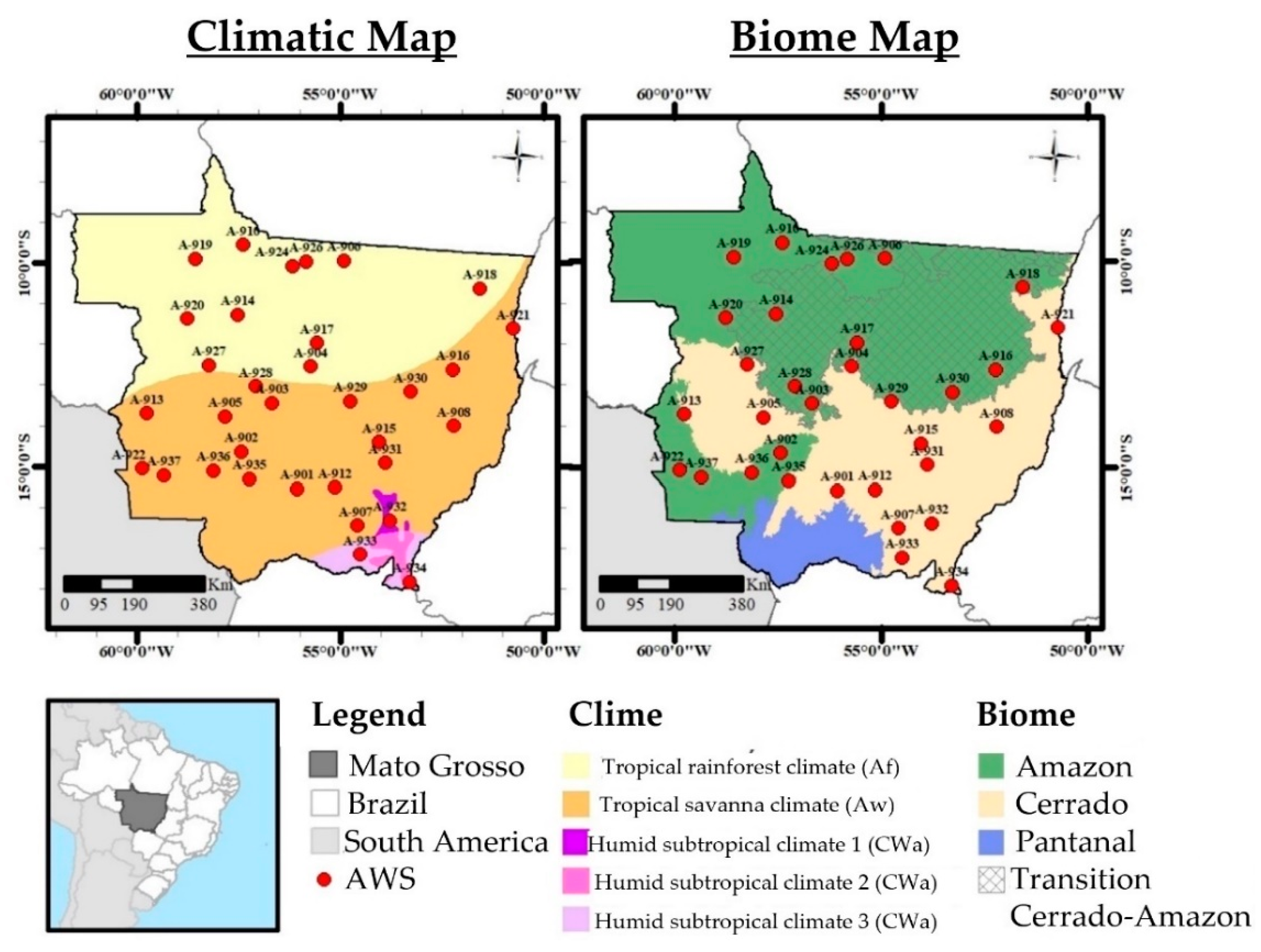
Figure 3.
Bias performance metrics, root mean square (RMSE), Pearson correlation coefficient of the nine global climate models in monthly estimates of reference evapotranspiration between the years 2007-2020 in the locations of the 33 AWSs in the state of Mato Grosso, Brazil.
Figure 3.
Bias performance metrics, root mean square (RMSE), Pearson correlation coefficient of the nine global climate models in monthly estimates of reference evapotranspiration between the years 2007-2020 in the locations of the 33 AWSs in the state of Mato Grosso, Brazil.
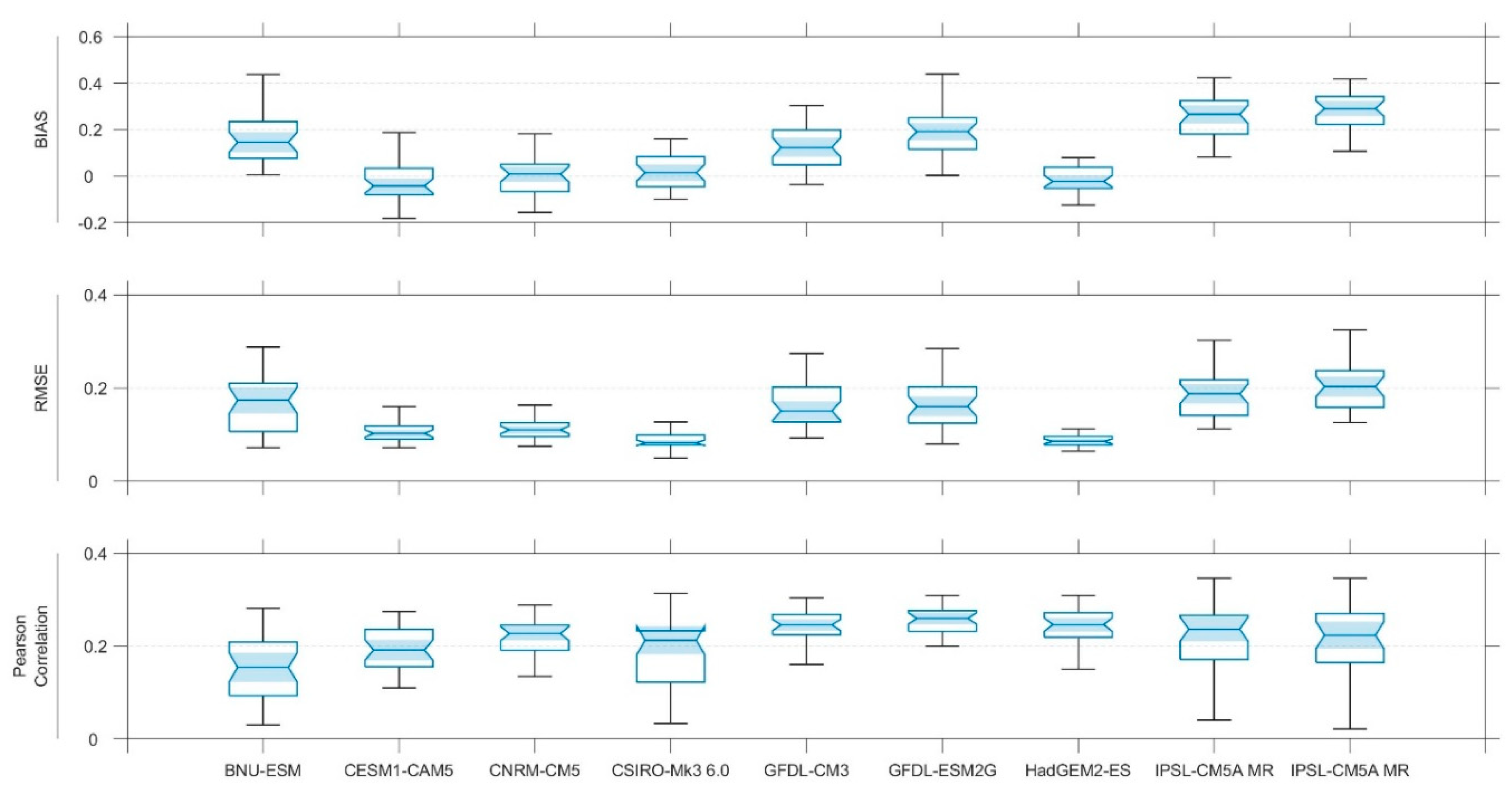
Figure 4.
5-year moving averages (line) and standard deviation (shaded area) of the reference evapotranspiration estimates and their meteorological variables projected by the HadGEM2-ES model in the RCP 2.6, RCP 4.5 and RCP 8.5 scenarios between the years 2007 and 2100 in the EMA locations in the state of Mato Grosso, Brazil.
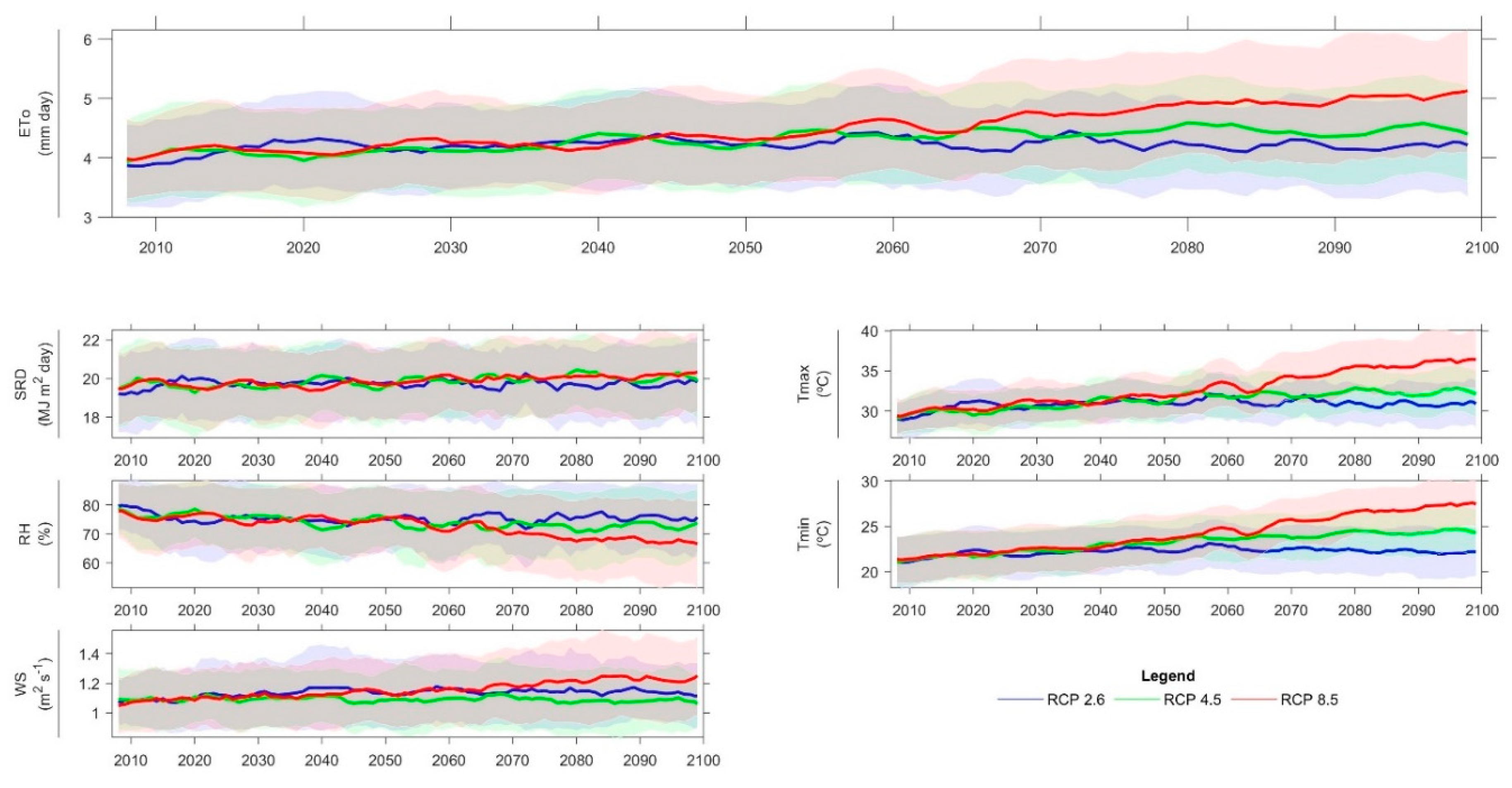
Figure 5.
Monthly variation of means and standard deviations of reference evapotranspiration estimates obtained by the HadGEM2-ES model in the three RCPs scenarios (2.6, 4.5 and 8.5, respectively) in four periods between 2007 and 2100.
Figure 5.
Monthly variation of means and standard deviations of reference evapotranspiration estimates obtained by the HadGEM2-ES model in the three RCPs scenarios (2.6, 4.5 and 8.5, respectively) in four periods between 2007 and 2100.
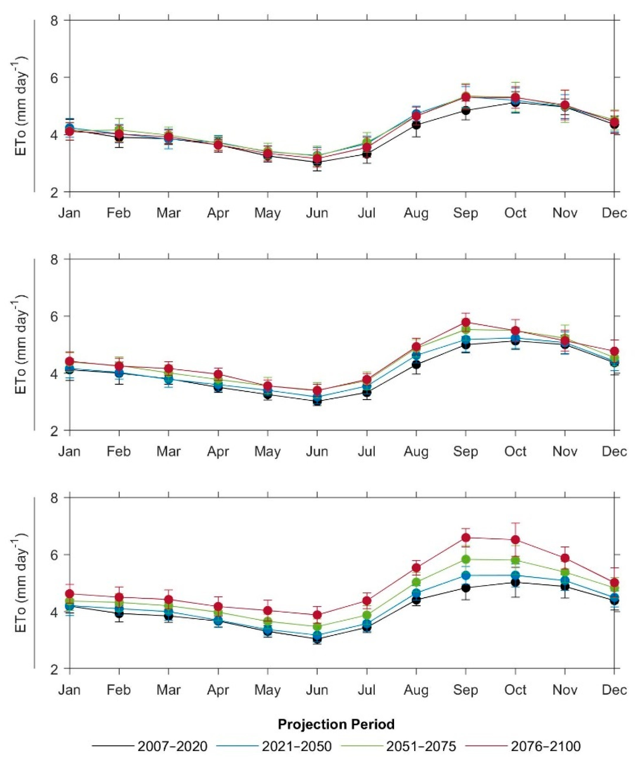
Figure 6.
Monthly averages of reference evapotranspiration (ETo) observed between 2007-2020, and estimates by the HadGEM2-ES model in the RCPs scenarios (3.6, 4.5 and 8.5) between the years 2007-2100, in the location of the AWSs of Mato Grosso, Brazil. NOTE: The difference between the level curves in the Figure is 0.2 mm day-1.
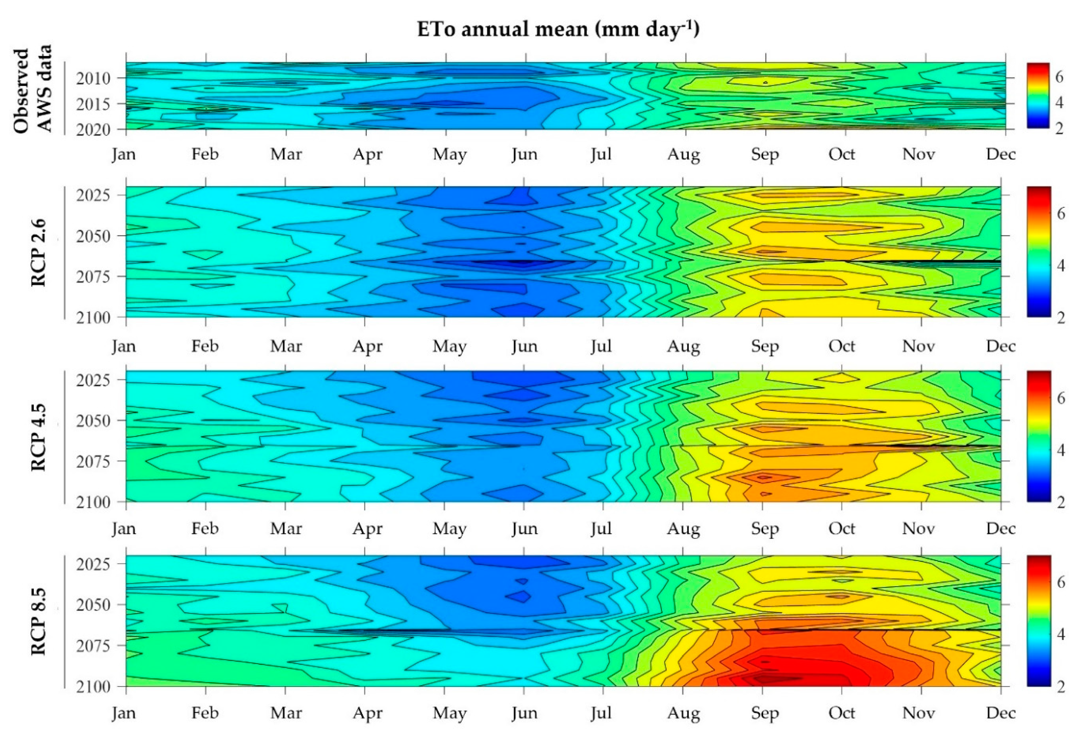
Figure 7.
Difference between the monthly averages of reference evapotranspiration (ETo) observed between 2007-2020, and estimates by the HadGEM2-ES model in the RCPs scenarios (3.6, 4.5 and 8.5) between the years 2025-2100, in the location of the AWSs from Mato Grosso, Brazil. NOTE: The difference between the level curves in the figure is 0.2 mm day-1.
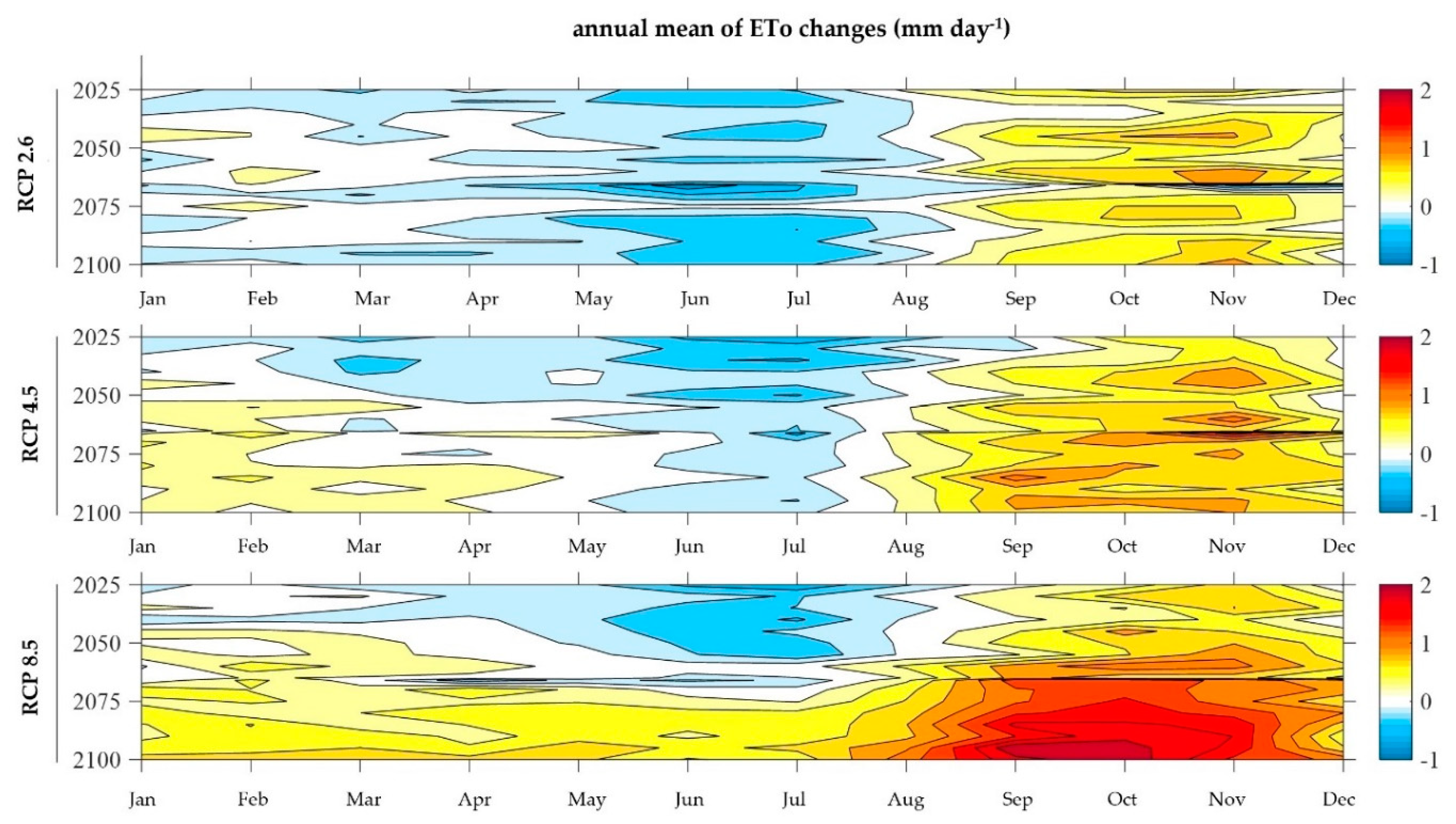
Figure 9.
Difference between the annual averages of reference evapotranspiration (ETo) observed in the AWSs of the state of Mato Grosso, between 2007 and 2020, and projected by the HadGEM2-ES model in RCPs 2.6, 4.5 and 8.5 scenarios in different periods of the 21st century. NOTE: Lines on the map demarcate the biomes and point to the AWSs in the state of Mato Grosso.
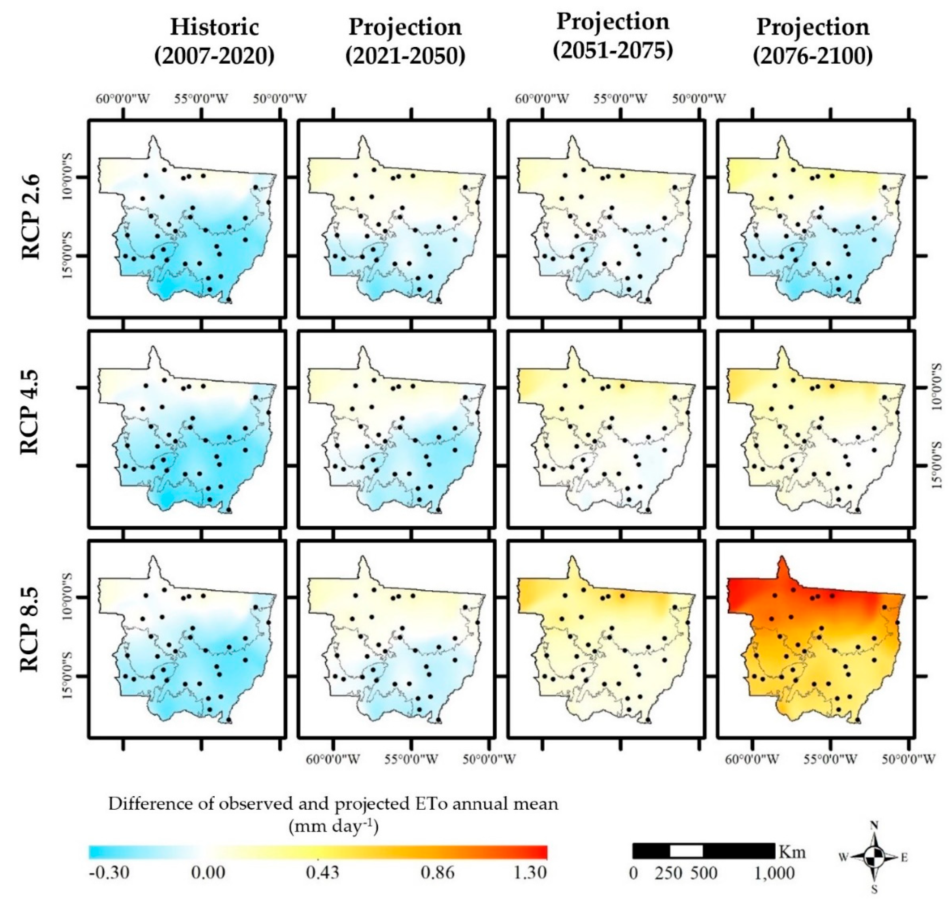
Figure 10.
Trends in reference evapotranspiration (ETo) and its meteorological variables observed in the AWSs of the state of Mato Grosso (2007-2020), and projected by the HadGEM2-ES model in RCPs 2.6, 4.5 and 8.5 scenarios (2007-2100). NOTE: Meteorological variables: SRD - net solar radiation; RH - relative air humidity; Tmax - maximum air temperature; Tmin - minimum air temperature; SW - wind speed at 2 m. Lines on the map demarcate the biomes and point to the AWSs in the state of Mato Grosso.
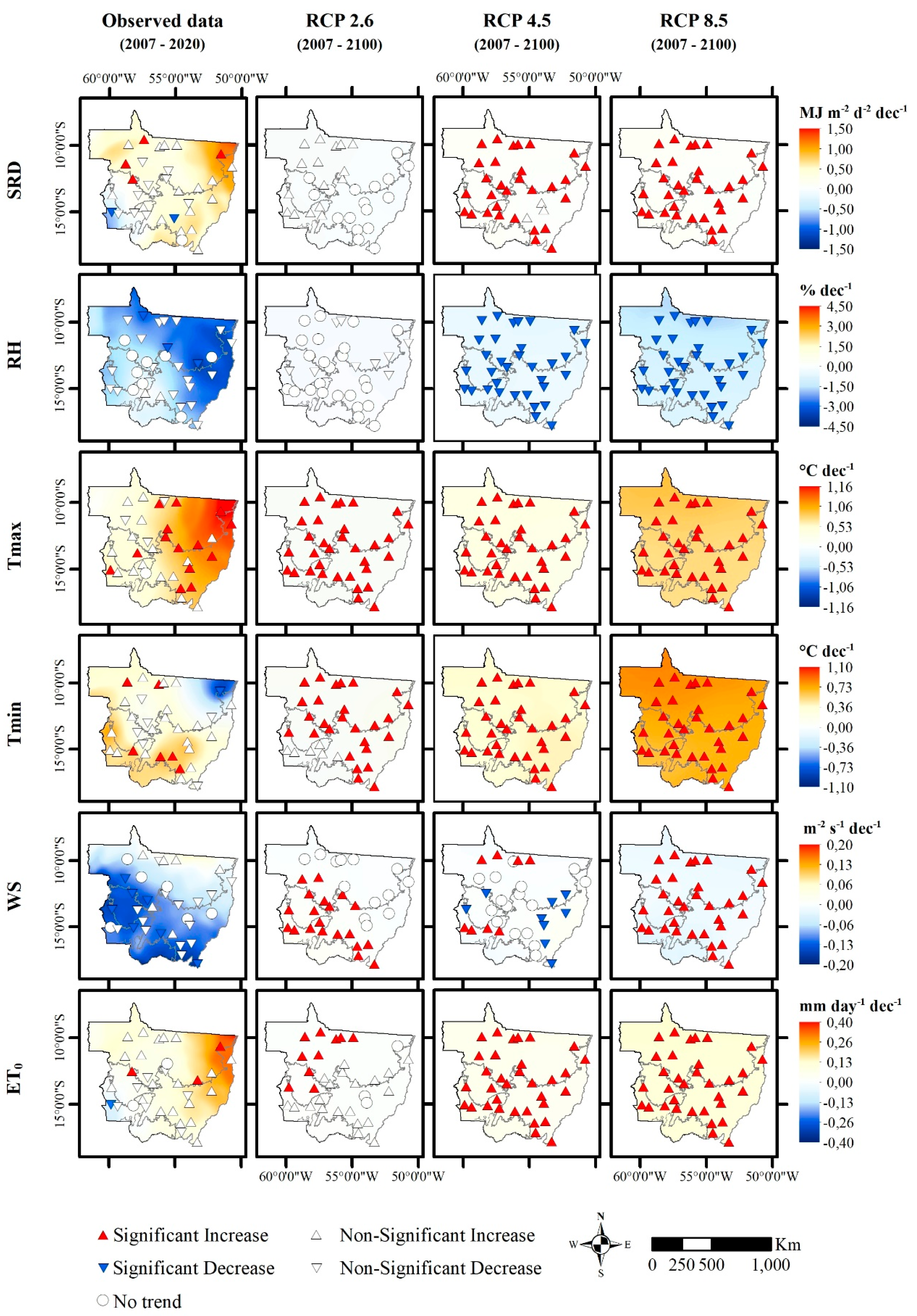
Table 1.
Global climate models (GCMs) were used in the study, along with their resolutions and responsible research groups.
Table 1.
Global climate models (GCMs) were used in the study, along with their resolutions and responsible research groups.
| MCG | Research Group | Resolution (Lat. × Lon.) |
|---|---|---|
| BNU-ESM | College of Global Change and Earth System Science, Beijing Normal University, China | 2.8 × 2.8 |
| CESM1-CAM5 | Community Earth System Model Contributors, USA | 1.25 × 0.94 |
| CNRM-CM5 | National Center of Meteorological Research, France | 1.4 ×1.4 |
| CSIRO-Mk3 6.0 | Organization/Queensland Climate Change Center of Excellence, Australia | 1.8 ×1.8 |
| GFDL-CM3 | NOAA Geophysical Fluid Dynamics Laboratory, USA | 2.5 × 2.0 |
| GFDL-ESM2G | NOAA Geophysical Fluid Dynamics Laboratory, USA | 2.5 × 2.0 |
| HadGEM2-ES | Met Office Hadley Center, UK | 1.88 ×1.25 |
| IPSL-CM5A LR | Institut Pierre Simon Laplace, France | 3.75 ×1.8 |
| IPSL-CM5A MR | Institut Pierre Simon Laplace, France | 2.5 ×1.25 |
Table 2.
Average annual reference evapotranspiration (ETo) from data observed in the AWSs of Mato Grosso and simulated by the HadGEM2-ES model in scenarios RCPs 2.6, 4.5 and 8.5 in four periods between 2007 and 2100.
Table 2.
Average annual reference evapotranspiration (ETo) from data observed in the AWSs of Mato Grosso and simulated by the HadGEM2-ES model in scenarios RCPs 2.6, 4.5 and 8.5 in four periods between 2007 and 2100.
| Eto (mm day-1) | Observed | RCP 2.6 | RCP 4.5 | RCP 8.5 |
|---|---|---|---|---|
| Actual (2007 – 2020) | 4.02 | 3.95 Aa | 3.94 Aa | 4.10 Aa |
| Projection (2021 – 2050) | 4.16 Aab | 4.13 Aa | 4.17 Aa | |
| Projection (2051 – 2075) | 4.13 Ab | 4.31 ABb | 4.42 Bb* | |
| Projection (2076 – 2100) | 4.08 Aab | 4.37 Bb* | 4.66 Cc* |
Means followed by different uppercase letters in the row and lowercase letters in the column differ statistically using the Kruskal-Wallis test at a 10% significance level. Averages followed by * differ from data observed between 2007 and 2020 in the AWSs in Mato Grosso.
Table 5.
Average reference evapotranspiration trend (ETo) and its meteorological variables (net radiation – SRD; relative humidity – RH; maximum temperature – Tmax; minimum temperature – Tmin; average wind speed – SW) observed in the AWSs of Mato Grosso, between 2007 and 2020, and projected by the HadGEM2-ES model in RCPs 2.6, 4.5 and 8.5 scenarios in the short term (2007-2020) and long term (2007 and 2100).
| Database | Period | Scenarios | Variables | |||||
|---|---|---|---|---|---|---|---|---|
| SRD | RH | Tmax | Tmin | SW | ETo | |||
| Observed | Short term (2007-2020) | Actual | -0.109 | -0.276 | 0.567** | 0.220 | -0.111** | -0.035 |
| Simulated | Short term (2007-2020) | RCP 2.6 | 0.731** | -4.709** | 2.141** | 1.216** | 0.016 | 0.423** |
| RCP 4.5 | -0.288 | -0.204 | 0.768 | 0.651** | -0.024 | 0.051 | ||
| RCP 8.5 | 0.047 | -1.211 | 0.683* | 0.587** | 0.047** | 0.075 | ||
| Long term (2007-2100) | RCP 2.6 | 0.006 | -0.084 | 0.080** | 0.058** | 0.005** | 0.011 | |
| RCP 4.5 | 0.061** | -0.539** | 0.345** | 0.377** | 0.001* | 0.055** | ||
| RCP 8.5 | 0.075** | -1.152** | 0.779** | 0.716** | 0.019** | 0.121** | ||
NOTE: Results followed by * or ** present significant trends using the Mann-Kendall test at 0.05 and 0.01, respectively. SRD – net solar radiation (MJ m-2 day-1 decade-1); RH – relative humidity (% dec-1); Tmax – maximum air temperature (ºC dec-1); Tmin – minimum air temperature (ºC dec-1); SW – average wind speed at 2 meters (m s-1 dec-1); ETo – reference evapotranspiration (mm day-1 dec-1).
Disclaimer/Publisher’s Note: The statements, opinions and data contained in all publications are solely those of the individual author(s) and contributor(s) and not of MDPI and/or the editor(s). MDPI and/or the editor(s) disclaim responsibility for any injury to people or property resulting from any ideas, methods, instructions or products referred to in the content. |
© 2024 by the authors. Licensee MDPI, Basel, Switzerland. This article is an open access article distributed under the terms and conditions of the Creative Commons Attribution (CC BY) license (http://creativecommons.org/licenses/by/4.0/).
Copyright: This open access article is published under a Creative Commons CC BY 4.0 license, which permit the free download, distribution, and reuse, provided that the author and preprint are cited in any reuse.


