
Submitted:
11 May 2024
Posted:
13 May 2024
You are already at the latest version
Abstract
Integrated energy systems (IES) seek to minimize power generating costs in future power grids through the dynamic coupling of different energy technologies. To accommodate fluctuations in load demand due to the penetration of renewable energy sources, flexible operation capabilities must be fully exploited, i.e., even power plants that are traditionally considered as base-load units need to be operated according to unconventional paradigms. Thermomechanical loads induced by frequent power adjustments can accelerate the wear and tear of components. If a unit is flexibly operated without respecting limits on materials and components, the risk of failures of expensive components will eventually increase, nullifying the additional profits ensured by flexible operation. In addition to the limits on power variations (explicit constraints), the solution of the unit dispatch problem needs to meet the limits on temperature, pressure and flow rate variations (implicit constraints). The FARM (Feasible Actuator Range Modifier) module was developed to enable existing optimization algorithms to identify solutions to the unit dispatch problem that are both economically favorable and technologically sustainable. Thanks to the iterative dispatcher-validator scheme, FARM permits addressing all the imposed constraints without excessively increasing the computational costs. In this work, the algorithms constituting the module are described, and the performance was assessed by solving the unit dispatch problem for an IES composed of three units, i.e., Balance of Plant, Gas Turbine, High-Temperature Steam Electrolysis. Finally, FARM module provides dedicated tools for visualizing the response of the process variables of interest during operation transients and a tool aiding the operator at making decisions. These techniques might represent the first step towards the deployment of an Ecological Interface Design (EID) for IES units.
Keywords:
Unit Dispatch problem
; Integrated Energy System
; Command Governor
; Ecological Interface Design
Introduction
Along with the benefits of reducing the carbon footprint and lessening the dependence on fossil fuels, the increasing penetration of renewable energy sources (RES) constitutes an issue for the stability of power grids. As a result of the limited dispatchability of solar power plants and wind farms, significant fluctuations in the net demand might lead to blackouts and interruption of service [1,2]. The deployment of RES, combined with the low cost and accessibility of natural gas, has led to a decrease in electricity prices, even resulting in negative values in some regions during periods of high RES production and low demand. Since the energy storage systems are not mature for grid-scale deployment [3], the only available approach is to enhance the operational flexibility of other power generation units connected to the grid. Even traditionally base-load units, e.g., nuclear power plants [4], need to be operated according to unconventional paradigms. The concept of Integrated Energy Systems (IES) aligns with this perspective. IES are cooperatively-controlled systems that dynamically apportion thermal and/or electrical energy to provide responsive generation to the power grid while also supporting the production of other energy products. Several research activities are currently carried on in Europe [5], in U.S. [6] and in China [7] to develop the IES technology. An IES unit combines conventional power plants with different characteristics in synergistic ways. For most units, electricity is considered the primary output, ensuring that grid demand is reliably met within the analysis region. Once electricity demand is met, the IES is designed to dynamically apportion any surplus primary energy to energy storage or to the production of industrial products. In some cases, the industrial product may be an intermediate energy carrier, such as hydrogen, or an intermediate chemical feedstock, such as methanol [8].
The problem of evaluating the mixed outputs of the generating units that minimize generation costs or maximize revenue is called unit dispatch. With regard to IES units, the goal of the unit dispatch problem consists of evaluating the power outputs and the heat flows that maximize the profitability of the whole system over the specified time horizon (days, weeks). It is a constrained optimization problem since limits on the minimum and the maximum power output along with the maximum ramp rate are imposed on all the power plants that constitute the IES unit. In this work, these limits are referred to as explicit constraints. Traditionally, unit dispatch problems are solved by adopting Dynamic Programming (DP) algorithms [9] or Mixed-Integer Linear Programming (MILP) algorithms [10]. These methods are effective for power plants that adopt current operational paradigms. The adoption of new operational paradigms requires the dynamic coupling between the power plants that constitute an IES unit. Thermomechanical loads caused by frequent power adjustments can accelerate the performance degradation and the wear and tear of components. If a unit is flexibly operated without respecting operational limits on materials and components, the risk of expensive components failures will eventually increase along with the frequency of maintenance interventions, nullifying the additional profits ensured by flexible operation. Let us consider the case of a nuclear unit. In Pressurized Water Reactors (PWRs), the condenser is the second-most expensive component of the entire plant after the reactor vessel [11]. To modulate the power output and effectively dispose of the heat produced in the core, the control actions governing the steam generator and steam turbine need to be coordinated. Along with the constraints on reactor power and turbine power, limits on the variations of pressure and moisture content in the turbine-discharged steam flow rate need to be imposed as well. Otherwise, the stress on the turbine blades and the condenser pipes will exceed design-basis conditions thus causing damage to the components. These limits are referred to as implicit constraints. Available tools need to be enhanced to formally account for implicit constraints. While necessary, adding numerous constraints on temperatures, pressures and flow rates increases the size of the optimization problem. In this work, an innovative approach for solving the unit dispatch problem for any set of generating units whose process variables need to be constrained during operation is presented and demonstrated. The key premise of the proposed approach is that solving the optimization problem by simultaneously considering both explicit and implicit constraints leads to prohibitive computational costs. A more efficient approach consists of addressing the optimization problem as a two-phase process. Similar to a Kalman filter [12], the proposed scheme has a prediction phase and an update phase. For the prediction phase, a traditional unit dispatcher finds a tentative solution that meets the explicit constraints on the power outputs. Such a tentative solution is then assessed by a sanity-check downstream of the unit dispatcher called "validator" (update phase). Its task consists of determining whether the tentative set-point trajectories are compliant with the implicit constraints on temperatures, pressures and flow rates. The embedded algorithm is the Command Governor (CG) [13,14]. It is a discrete-time device that is used in the field of feedback control of dynamic systems. Although CG is typically used as a supervisory control algorithm, this work proposes an innovative application for it, i.e., aiding the solution of the unit dispatch problem for complex mixed-generation plants. Thanks to a model of the studied system, the unit response to demanded power transients can be evaluated, and possible violations of the imposed limits are identified and returned to the unit dispatcher. The algorithm is recursive, i.e., the solution of the optimization problem will be approved only when all the constraints are met.
Widely used to describe the safe operation of a power plant, a turbomachinery or any engineering system, the Normal Operation Region (NOR) is defined as the ensemble of operating points at which the system can function without exceeding design-basis conditions of its components [15]. Having identified p process variables whose evolution needs to be limited to preserve the integrity of system components, the NOR can be mathematically defined as a p-dimensional polytope in the phase space [16]. The validator’s task then consists of ensuring that the power demanded for the plants constituting the IES unit do not lead the corresponding process variables to violate the NOR bounds. In Figure 1, a qualitative representation is shown. The dashed green trajectory describes an acceptable unit response during a power transient, i.e., the entire trajectory lies within the NOR bounds (blue region). In case operating conditions exceeds the NOR bounds, the components will experience excessive thermomechanical loads, thus increasing the risk of failure over time (orange region). Ultimately, if a transient pushes the system even further, the safety variable limits (solid black line) will be breached, potentially leading to a severe accident. The proposed scheme provides a quantitative estimate of the NOR, i.e., the constraints on the process variables are "translated" into limits on the power set-point trajectories. As a major outcome, it provides a tool that conveys the major information about the plants conditions in a simple and straightforward fashion.
The paper is organized as follows. In Section 1, the new approach to the solution of the unit dispatch problem for IES units and the role of the validator are presented. In Section 2, the modeling framework implementing the proposed scheme is described. In Section 3, the algorithms embedded into FARM for predicting the system response, detecting the constraint violations and corrective actions are described. In Section 4, the IES unit selected as a test case is described, and the constraints enforced during operation are listed. In Section 5, the steps that lead to the solution of the unit dispatch problem for the studied system are defined, and the obtained results and the associated computational costs are discussed. In Section 6, visualization techniques for displaying the IES unit response during power transients are presented, and a possible role of FARM as aid to unit operators is proposed. Finally, the main conclusions are drawn and future steps are discussed.
1. Description of a New Approach to the Solution of Unit Dispatch Problems
As mentioned in the Introduction, when solving the unit dispatch problem for an IES unit, there are two sets of limits that need to be respected, i.e., explicit constraints and implicit constraints. Any solution of the unit dispatch problem that both meet these two sets of constraints is defined as a feasible solution.
- Explicit constraints: the electrical power output can assume any value within a characteristic window, i.e., (power output limits). Electrical power variations cannot be too steep either, i.e., (power ramp-rate limits). Explicit constraints are also defined as low-resolution physics constraints because they represent fewer physics details.
- Implicit constraints: to prevent thermomechanical loads from surpassing the design limits, constraints on temperature, pressure, and flow rate must be taken into account, i.e., , , and . Implicit constraints are also defined as high-resolution physics constraints since they account for a large number of aspects that govern the processes.
Ideally, all these constraints should be addressed by the unit dispatcher (Figure 2a). Unfortunately, the size of the ensuing optimization problem would entail a large computational burden. The problem could be addressed by splitting the two sets of constraints, i.e., the unit dispatcher will address the explicit constraints for each unit, and the corresponding control systems will address the implicit constraints by imposing saturation limits on the PID controllers (Figure 2b). By adopting this method, the set-points issued by the unit dispatcher will never cause the violation of implicit constraints of the IES unit components, and the size of the optimization problem will be manageable since the unit dispatcher only addresses the explicit constraints. However, the resulting power transients will be sub-optimal and there is the possibility that the load demand will not be met [17].
The approach proposed in this work consists of solving the constrained optimization problem by placing a sanity-check downstream of the unit dispatcher to ensure the feasibility of the found solutions. The CG was identified as a suitable algorithm to fulfill this task. It is an add-on scheme that enforces pointwise-in-time constraints by modifying the set-point signals fed to a closed-loop, dynamic system. The problem of designing the control system is then addressed as a two-step process. The primal regulator is tasked to stabilize the system and provide tracking properties in the absence of constraints. It can be a set of traditional feedback regulators, e.g., PID controllers. The constraint fulfillment task is left to the CG, i.e., a nonlinear device which is added to the primal compensated nonlinear system. Whenever necessary, the CG modifies the reference set-point signal supplied to the primal regulator to enforce the fulfillment of the constraints [18]. Originally conceived as a layer of control system architectures, the CG is used in this work to speed up the constrained optimization process. As mentioned in Introduction, the CG "translates" the implicit constraints into explicit constraints, thereby imposing more restrictive limits on the set-point trajectories. Updated limits aid the dispatcher in identifying an optimal solution that conforms to both sets of constraints.
The proposed approach is composed of the following five steps:
- The capacities of the IES unit subsystems (i.e., maximum power output/consumption) are defined by the user;
- Given the subsystem capacities, the HERON dispatcher solves the constrained optimization problem by approximating the optimal power output/consumption for each subsystem. These trajectories () satisfy the explicit constraints (Figure 3);
- The CG determines if the trajectories calculated by the HERON unit dispatcher satisfy the implicit constraints as well. If not, the CG will provide trajectories complying with both explicit and implicit constraints (), and return them to the unit dispatcher for re-optimization;
- From trajectories, the HERON dispatcher derives a feedback to adjust the values of the explicit constraints. The outputs of the single subsystem are modified accordingly;
- Steps (2) through (4) are repeated until and are identical, i.e., the optimal trajectories satisfying heat and electrical power demands are also compliant with both explicit and implicit constraints. The “approved” set-points are then issued to the PID controllers that calculate the control actions () to simulate the prescribed power transients.
In Figure 4, a detailed view of the feedback provided by the Validator to the Unit Dispatcher is shown. For simplicity, the optimization of a single power set-point is depicted. Once the system’s evolution in response to has been simulated, the margins with respect to the lower and upper bounds on process variables are evaluated, "translated" into margins on the bounds of production variables (i.e., electrical power, in this case), and returned to the Unit Dispatcher. In Figure 4, they are outlined in red as . These contributions will be added to the explicit constraints ( and ). In this way, a more comprehensive characterization of the feasible system capabilities is obtained. The final constraints ( and ) will include both the inherent limits on standalone subsystems performance (expressed by the explicit constraints) and the additional, more restrictive limits resulting from the interactions with other interconnected subsystems, typical of the IES unit configuration (expressed by the "translated" margins). The adopted scheme does not cause any issues with the convergence of the optimization process. The unit dispatch problem being addressed is the traditional one. The inclusion of the Validator only provides additional contributions to the constraints on the production variables. Specifically, it reduces the space of feasible solutions in which to search for the optimal one.
2. Description of the Modeling Framework for Solving the Unit Dispatch Problem for IES Units
In this work, the scheme outlined in Section 1 was implemented to address the unit dispatch challenge for an IES. The IES units are constituted by thermally-coupled power plants designed to operate in synergistic ways. Due to their complex configuration and the necessity for component coordination, IES units incur higher initial and operational costs compared to standard energy systems. Assessing the financial viability of such investments involves analyzing the economic performance over their operational lifespan that spans several decades. Such analysis requires an unprecedented modeling and simulation effort to ensure the proposed operational paradigm will not cause damages to components or materials. To achieve this goal, a research program was started in 2015 [6,8], focusing on integrated modeling, simulation and experimental facility development. Consequently, a comprehensive framework named FORCE (Framework for Optimization of Resources and Economics) was established[19], integrating and enhancing tools from various software to cater to the specific requirements mentioned.
- RAVEN (Risk Analysis Virtual Environment) is a multipurpose uncertainty quantification (UQ), regression analysis, data analysis and optimization framework [20]. RAVEN is the central engine for the deployment of all the analysis needs, providing the tools for the construction of the analysis workflows. RAVEN is charged with deploying the optimization methodology and algorithms that are used for the capacity optimization. In addition, the framework delivers the techniques for the generation of synthetic scenarios via its time series generators [21]. The capability of generating synthetic scenarios based on existing grids, starting from available datasets, is crucial. In this way, hypothetical scenarios characterized by larger penetration of renewable energy sources or higher level of variability in the demand profile can be investigated.
- HYBRID software is a collection of component models developed primarily using the Modelica language and deployed using the Dymola software suite [22]. An IES unit is constituted by traditional power plants whose dynamics are characterized by very different time constants, i.e., along with a nuclear power plant, there are gas turbines that can be started up from cold shutdown conditions in 20 minutes. To obtain a realistic description of the system performance, the capability of accurately simulating the dynamic response of the IES components over different time scales is crucial. HYBRID contains low-fidelity and high-fidelity models for all the energy systems and components that have been selected as part of the IES framework.
- HERON (Holistic Energy Resource Optimization Network) is a plug-in that allows performing stochastic full-system techno-economic analysis of grid energy-resource systems with economic drivers [23]. The development targets analysis of electricity and secondary product generation and consumption in regional balancing areas, including flexibility to include arbitrary resources as well as arbitrary resource consumers and producers. HERON is the tool for the construction of the overall IES/FORCE workflow, providing tools for deploying systems’ dispatching strategies and capacity optimization.
- TEAL (Tool for Economic AnaLysis) is a discounted cash flow analysis plug-in that allows for a generic definition of cash flows, with drivers provided by RAVEN. It includes flexible options to deal with taxes, inflation, discounting and offers capabilities to compute a combined cash flow for components with different component lives [24]. TEAL is tasked with deployment of the economic analysis within the IES methodological framework.
In Figure 5, the graphical representation of the FORCE workflow is shown. At the top, the HERON module is represented. The result of the techno-economic analysis includes the dispatching strategy, i.e., the set of power output and the heat flux set-points for the energy systems that constitute the unit. At the bottom of Figure 5, the HYBRID module is represented. The embedded Dymola model of the IES unit is used to simulate the power transients that are prescribed by the set-point trajectories provided by HERON. In addition, the Dymola model can be run off-line to generate data-sets characterizing the dynamics of the IES unit. Between this two modules is the validator assessing the tentative dispatching strategies. The developed validator module is named FARM (Feasible Actuator Range Modifier) [25], which bridges the high-fidelity (HYBRID) and low-fidelity (HERON) description of the IES unit. In Figure 6, a graphical representation is shown.
To detect possible violations of implicit constraints, every time a power or heat flux set-point changes, the response of the IES unit components needs to be estimated by adopting a reduced order model of the unit and the corresponding control system. For this kind of applications, Linear time-invariant (LTI) state-space models are often adopted (Eqs.(1)(2)).
In this work, the unit response to tentative set-points is estimated by using a Linear parameter-varying (LPV) model [26]. An LPV model is constituted by a set of LTI models obtained by linearizing the set of Differential-Algebraic Equations (DAEs) [27] describing the dynamics of the studied system around anchor points in the scheduling space called scheduling parameters (Eqs.(3)(4)). In the current implementation, the set of matrices corresponding to the LTI models are indexed by the corresponding production level.
where , , and are the state-space matrices parametrized by the scheduling parameter vector .
To build the LPV model, a data-driven method was implemented in FARM. As a first step, a dataset containing the IES unit responses during multiple power transients must be generated. These data may be either measurements collected from the actual unit or simulations generated by running a high-fidelity model of the unit. These latter solution can be significantly facilitated by the use of the FMI/FMU standard [28]. The Functional Mock-up Interface (FMI) defines a standardized interface to be used in simulations that simplifies the creation, storage, exchange, and (re-) use of dynamic system models. With such an interface implemented, the Dymola model can be exported as an executable called an FMU (Functional Mock-up Unit), which can be imported into other supported environments for simulation. An FMU may either encapsulate its own solvers (FMU for Co-Simulation) or require the simulation environment to perform numerical integration (FMU for Model Exchange) [22,29]. The high-fidelity model used in this work to generate the simulation data was developed in the Dymola simulation environment. After building the model of the studied IES unit by assembling the components models from the HYBRID library, it was exported into a Co-Simulation FMU and used within FARM (Figure 6). The FMU receives set-point trajectories and returns the responses of all the process variables. The simulation results were then collected in a database and used to derive the LPV model.
To help solve the unit dispatch problem, FARM operates in two consecutive phases. The described procedure for deriving the LPV model is performed during an off-line phase called Self-Learning. After generating the LPV model, the unit dispatch problem is solved during the on-line phase called Dispatch. HERON first issues power set-point trajectories meeting the explicit constraints, which represents low-resolution physics. FARM simulates these power transients using the LPV model and evaluates the margins of the process variables relative to the corresponding implicit constraints, which represents high-resolution physics. These margins are then "translated" into margins on the explicit constraints () and returned to HERON (Figure 6). In this way, the information on constraint enforcement can be used during the next iteration of the dispatch optimization process. These iterations between HERON and FARM during the Dispatch phase are necessary to find a solution that meets both explicit and implicit constraints. In this scheme, the task of the LPV model consists of predicting the response of the studied system during transients and notifying possible constraint violations. In addition, the procedure implemented in FARM module ensures the LPV model the capability to "learn" during the solution of the unit dispatch problem. In case the FMU is coupled with HERON-FARM optimization scheme, real-time data are collected during the Dispatch phase, and new matrices are derived and added to the LPV model developed during the Self-Learning phase. In this way, the latest, most accurate mathematical description of the system dynamics are available. Inevitably, this procedure results in an increased computational burden. In this work, this capability was not utilized, i.e., no FMU was integrated with the HERON-FARM optimization scheme during the Dispatch phase, and the LPV model developed during the Self-Learning phase was not improved thereafter. Finally, when demonstrating the capabilities of the scheme by solving a unit dispatch problem (Section 5), the response of the IES unit is simulated by using the LPV model.
3. Description of the Algorithms Embedded in FARM
In this Section, a brief overview for each of the algorithms embedded into FARM module is provided. For a more complete description of of these tools, the reader is referred to dedicated references.
- Command Governor: it performs a multi-dimensional optimization of set-point trajectories fed by the unit dispatcher (Section 3.1).
- Convex Hull: it removes the redundant constraints (Section 3.2)
- Dynamic Mode Decomposition with Control: it derives the matrices that constitute the state-space model (Section 3.3).
- Recursive Feature Elimination with DMDc: it provides the list of state variables of the derive state-space model (Section 3.4).
3.1. Command Governor (CG) for Enforcing Implicit Constraints
The CG algorithm adjusts the vector reference signal () to produce a feasible set-point signal () to be fed to the feedback regulators. The goal is deriving set-point trajectories that will start power transients that meet the imposed constraints. In this Section, a description of this algorithm is provided. For further information, the reader may refer to [30,31]. The CG is based on an iterative, finite-horizon optimization scheme. At time , the current state of the system is sampled and a feasible set-point value is calculated for a relatively short time horizon , where g is a positive integer representing the number of time-steps that constitute the time horizon. An online calculation is used to explore state trajectories from the current state () to the end of time horizon (). After the first step of the optimized set-point trajectory is fed to the PI controllers, the state is sampled again and the calculation is repeated, yielding a new value. The key concept behind the CG algorithm is the definition of a feasible region for the adjusted set-point values at time . Any vector laying within this region can be imposed as system set-point at time and remain constant over the time horizon, without causing the constrained process variables to violate the imposed limits over the same time horizon. The CG algorithm shares several similarities with the Model Predictive Control (MPC)[32]. Although both algorithms optimize the actions governing the dynamic system over a finite time horizon that shifts forward at every time-step, they operate at different levels. The MPC replaces traditional PID controllers by optimizing the actions executed by the actuators to meet targeted specifications, e.g., tracking capabilities, asymptotic stability, and constraint enforcement; the CG "collaborates" with the PID controllers, i.e., it optimizes the set-point trajectories to ensure constraint enforcement, whereas the PID controllers guarantee good tracking capabilities and asymptotic stability. It is a two-step approach that does not alter the traditional control system architecture.
Let us consider a system characterized by p output variables () and assume that the lower and the upper limits on these variables can be represented by a set of linear inequalities, i.e., and (Eq.(5)).
First, let us impose that the constraints are not violated at the current time-step (). By adopting Eq.(5), Eq.(4) can be written as Eq.(6).
Then, the feasibility of the set-point trajectory needs to be assessed for the following time-steps as well. Once and matrices are defined (Eq.(7)), the linear inequalities can be re-written as shown in Eq.(8).
The feasible region is defined by all the linear inequalities in Eq.(6) and Eq.(8). Eq.(3) is adopted to express Eq.(8) in terms of the current state variables (Eq.(9)).
where
Eq.(8) can be expressed in terms of the current state variables values () by iteratively performing the same derivation (Eq.(11)).
In Eq.(12), the constraints expressed in Eq.(5) evaluated between and are assembled. They constitute the MOAS (Maximal Output Admissible Set), i.e., the admissible region for the vector of adjusted set-points at time . The corresponding matrix equation is reported in Eq.(13).
Geometrically, the MOAS defines a m-dimensional convex polytope. Each vector laying within this polytope is a feasible solution to the constraints enforcement problem (Eq.(5)) [33]. In Section 0, the concept of NOR was presented. The NOR was defined as a p-dimensional polytope defined by the set of constraints imposed on the major process variables. Given the meaning of the MOAS, the relationship with the NOR can be immediately identified. The NOR is the feasible region for the constrained process variables of the system, and it is defined in a p-dimensional phase space. The MOAS is the feasible region for the adjusted set-points that do not lead to forbidden responses of the output variables, and it is defined in a m-dimensional space. The CG "translates" the constraints on the process variables into limits on the set-point trajectories, i.e., the NOR defined in the p-dimensional space is replaced by a region in the m-dimensional space that is equivalent from the description of the system dynamics standpoint. As a major outcome, the CG allows deriving a procedural definition of the NOR that can be implemented into an algorithm for optimizing the operation of a unit such as a power plant. To find the optimal solution, the CG solves a Quadratic Programming (QP) optimization problem [34]. As shown in Eq.(14), the goal consists of calculating an adjusted set-point trajectory that is as close as possible to the reference one.
With regard to the application of FARM to the solution of the unit dispatch problem, in the current formulation, the power and heat flux set-points are adjusted on hourly basis. Accordingly, the length of the prediction horizon should cover the whole hour. At the same time, the time constants governing the dynamics of the power plants that constitute the IES unit are not so long, i.e., the operational transients initiated by set-point variations are considered completed before the end of the hour. Still, the prediction horizon is imposed equal to one hour to be conservative, i.e., the CG will adjust the set-points to enforce constraints throughout the entire hour.
3.2. Convex Hull Method for Removing Redundant Constraints
When defining the unit dispatch problem, implicit constraints are imposed to limit the thermomechanical loads. Since the components that constitute the IES unit of interest are thermally coupled, the constraints on the process variables of one component might affect the operation of another component. As a result, some constraints defining the MOAS might be redundant. If they are not removed, they will increase the computational burden and cause the QP solver to return a sub-optimal solution [35]. To address this issue, a procedure borrowing the “convex hull” concept from geometry [36] was implemented in the FARM module. The expression of the normalized MOAS for m-dimensional actuator signal with q constraints is reported in Eq.(15).
Assume that both H matrix and h vector are normalized, i.e., all the rows of H matrix have the same magnitude (Eq.(16)).
Eq.(15) defines an m-dimensional convex polytope. Once an inner point () is found meeting all the q constraints, a translatory motion is performed to include the origin point (Eq.(17)).
where .
It is worth stressing that the origin point () is within the m-dimensional polytope defined by Eq.(18), i.e., . A new matrix M is defined as the element-wise division between and (Eq.(19)),
The row of M matrix is an m-dimensional vector. Its direction follows the m-dimensional normalized vector composed by the numerators (Eq.(20)). Its magnitude is inversely proportional to the value of .
The Convex Hull is built by using all the q rows of m-dimensional vectors. Among all the m-dimensional vectors that share the same direction, the one with largest magnitude (smallest values of ) corresponds to the tightest constraint. This property can be used to define a ranking criterion. The convex hull is the smallest convex set that contains all the provided points, i.e., the points on the vertices of such convex polytope correspond to the tightest constraints in MOAS. For visualization purposes, the convex hull corresponding to the test-case reported in [37] was built. An IES unit constituted by two power plants, i.e., a Rankine energy conversion cycle and a turbine cycle, is considered. The unit dispatch problem consists of optimizing the corresponding power outputs at the beginning of each hour to meet the load demand for electrical power. In a discrete-time domain (10 second time-steps are adopted), the built MOAS has 2,888 rows, where the 2 bounds (upper and lower bounds) of 4 monitored variables over 361 time-steps are described. Hence, the M matrix has 2,888 rows of 2-dimensional vectors (blue points in Figure 7). The four blue points on the vertices of the convex polygon correspond to the 4 tightest constraints in MOAS, whereas all the other 2,884 blue points inside the polygon correspond to constraints that can be dropped.
The ConvexHull function is available from the scipy python package [38]. It allows constructing a convex hull from a given M matrix and returning the indexes of the points on the vertices which correspond to the non-redundant constraints in MOAS. The final set of constraints is equivalent to the original MOAS. Consider the results reported in Figure 8. The original 2,888 constraints and the reduced 4 non-redundant constraints define the same feasible region of multi-dimensional actuators. In addition to the reduced computational burden, the convergence to the optimal solution has improved. When too many redundant constraints are provided, the QP solver is challenged, and a sub-optimal solution is returned occasionally (black square in Figure 8a). Thanks to the convex hull method, the returned solution is within the feasible region and has a minimized distance from the original actuator (black square in Figure 8b).
3.3. Dynamic Mode Decomposition with Control for Deriving the State-Space Matrices
As mentioned in Section 2, FARM needs a state-space model to predict the IES unit response during operational transients and to avoid recommending dispatch variations that could compromise component integrity. Models based on the solution of first-principle equations are preferred as they can accurately describe a wide range of operating conditions without any training datasets. However, when a power plant is operated, physical parameters (e.g., thermal resistances, friction factors, etc.) evolve in time because of inevitable degradation phenomena. As a result, the dynamics of the system is impacted, leading the model to become outdated over time. The effectiveness of the constraint enforcement algorithm, which depends on the accuracy of model predictions, will consequently decline. In the process of developing tools to aid the solution of the unit dispatch problem in real-world scenarios, the latest, most accurate description of the system conditions and dynamics, i.e., an actual Digital Twin (DT) that mimics the system behavior in response to performed control actions, is necessary. FARM uses a system identification method that allows deriving the state-space model of the studied system from the measurements of the main process variables. In particular, the state matrix () and the input matrix () of the state-space model in discrete time domain (Eqs.(1)(2)) are calculated by adopting the Dynamic Mode Decomposition with Control (DMDc) [39]. The matrices are constructed by collecting temporal snapshots of the system inputs () and state variables () over discrete time-steps (), as shown in Eq.(21).
Since the derived matrices represent the best-fit solution for the data contained in the training data-set, the relationship in Eq.(1) does not exactly hold. It can be rewritten in a matrix form to include the new data matrices.
To solve Eq.(24), the Singular Value Decomposition (SVD) is applied to the augmented data matrix (Eq.25).
where , and are the truncated SVD components. The truncation value q is the number of non-zero elements in . In this work, the truncation value q is set to limit the condition number of matrix to below . Eq.(26) provides an approximation of G.
By breaking the linear operator into two components according to the dimensions of and , the estimates of and matrices can be found (Eq.(27)).
where and .
To complete the state-space model, and matrices need to be derived. Given the nature of the studied systems, the input vector has no direct impact to the system output, i.e., matrix is zero. To find the best-fit solution of the matrix using the system state vectors and system output vectors in the training data set, the matrix of temporal snapshot of system output vector is constructed (Eq.(28)).
3.4. Recursive Feature Elimination for Selecting the State Variables
To derive the matrices that constitute the state-space model, the DMDc tracks the responses of the state variables during operational transients. The state variables of a dynamic system are defined as the minimum set of process variables that allows predicting its future behaviour in response to any given set of inputs. If an analytical model is not available, identifying the state variables from the pool of process variables is not trivial. Many commonly-used algorithms for deriving state-space models only reconstruct the relationship between input and output variables (regression models). The main limit of these methods is that the state variables of the derived models have no physical meaning, i.e., their number is determined by the quality of the curve-fitting on the training data-set [41]. In [42], Recursive Feature Elimination (RFE) was adopted to identify a single, exhaustive set of process variables for a system constituted by multiple subsystems interacting with each other. This automated procedure for state variable selection was implemented into the FARM module. As shown in Figure 6, the optimal set of process variables is identified and their evolution is tracked to derive the LPV state-space model. In this Section, a brief overview of the scheme is reported.
The cost function accounting for the accuracy of both state variable and output variable predictions is defined as follows. Let us consider n candidate state variables and p output variables. The known values of the candidate state variables () and the output variables () are contained in the training data-set. The predicted values of the candidate state variables () and output variables ) are calculated by using the trained matrices (, and ), the input variable trajectory (), and the initial values of the candidate state variables (). and represent the standard deviations of the dimension of the known state variables and the dimension of the known output variables, and they are used for normalization purposes. The cost functions is obtained by summing the weighted mean square error (MSE) between the predicted values and the known values of the candidate state variables and the weighted MSE between the predicted values and the known values of the output variables calculated over l time-steps (Eq.(31)).
The RFE is a well-known tool that has been extensively adopted to develop feature-ranking methodologies for dimensionality reduction applications [43]. The procedure adopted in FARM for selecting the state variables is iterative, and it consists of the following steps:
- Construct an evaluation model, trained on a complete feature space data-set.
-
Rank the features by using one of the following method:
- (a)
- Sensitivity ranking method (ranking of the features based on their sensitivity coefficients);
- (b)
- Correlation ranking approach (ranking of the features based on their correlation coefficients);
- (c)
- A model-based importance ranking method exploiting the mathematical formulation of the evaluation model (e.g., linear model coefficients, etc.).
- Remove the features with the lowest scores calculated by the selected ranking criterion.
- Repeat the process until the user-defined number of variables are selected.
The RFE method is an instance of backward feature elimination. To reduce the computational time, multiple features are removed during each iteration. The method produces a feature subset ranking, as opposed to a feature ranking. Feature subsets are nested . To achieve the higher efficiency while avoiding the fitting issues caused by the collinearity between candidate variables, a hierarchical clustering pre-filtering [44] was then deployed. The development of an automated approach to state variable selection based on RFE was driven by the observation that the matrix is a transfer operator from the state space to the output space of the evaluation model. Once normalized by using a min-max scaling approach, the matrix is used to assess the importance of the candidate state variables (features) with respect to the output variable(s). The importance matrix is defined as follows:
where:
- is the original value of the element in the row and column of ;
- is the row of ;
- and are the minimum and maximum values in the row of , respectively.
Once importance matrix is evaluated, a "score" for each state variable is derived by calculating the expected value of the importance matrix along each column (Eq.(33)). The candidate state variables are then ranked by this score, i.e., the variables with the lowest scores are eliminated. The importance matrix and the scores are updated at each iteration of the feature elimination process, until the desired number of variables is reached.
Let us consider a dynamic system constituted by two subsystems, A and B (Figure 9) and assume that N process variables () are recorded for subsystem A, and M process variables () are recorded for subsystem B. The goal is to select the state variables of the coupled system, i.e., the minimum set of process variables describing its dynamics (), where and .
Initially, the RFE-based scheme was applied to the entire set of process variables, without discriminating between the subsystems. The results were not satisfactory, i.e., most of the selected variables belonged to a single, high-impact subsystem. To ensure an unbiased selection, an alternative importance-ranking methodology was proposed. The main steps are described below.
-
Step IThe RFE selection is performed on each subsystem, i.e., A and B are independently studied. At the end of this stage, the two sets of candidate state variables for subsystems A and B are selected ( and ).
-
Step IIThe two sets of recorded process variables are analyzed with a cross-correlation technique. This step is crucial even when the subsystems are not interacting since the process variables of a subsystem can be "privileged", being characterized by a higher scores through the importance metrics (Eq.(33)). The influence that variables perform on the candidate state variables () and the output variables () of B is evaluated and vice versa. It is worth stressing that the impact on both the candidate state variables and the output variables needs to be accounted for (Eqs.(34)(35)). As a result, two new sets of candidate state variables are obtained ( and ).
-
Step IIIA cross-system set of candidate state variables is generated (). The optimal set () is evaluated by maximizing the accuracy of the model in reconstructing the state variable and the output variables spaces. A parallel searching is then performed over all the combinations of the cross-system set of candidate state variables by minimizing the cost function (Eq.(31)).
4. Description of the Test-Case System and Operational Constraints
To demonstrate the capabilities of the FARM module, an IES comprising three subsystems was adopted as a test case. As shown in Figure 10, a steady superheated steam flow rate () is generated by a nuclear reactor and shared between a Balance of Plant (BOP) and a High-Temperature Steam Electrolysis (HTSE) process through the Energy Manifold (EM). The primary purpose of this flow rate is to generate electricity in the BOP (). A significant portion of the steam flow rate () is then channeled towards the BOP to be expanded in the steam turbine. After meeting the load demand (), any excess steam () and any excess power () are used to feed the hydrogen production process in the HTSE. The rate value of the steam flow rate () is not sufficient for operating both the BOP and the HTSE at full capacity simultaneously, i.e., the steam distribution between the two thermally coupled subsystems needs to be properly coordinated. To avoid abrupt pressure variations, a single directional steam sink with prescribed pressure (not shown in Figure 10) is connected to the EM (). In addition, a Gas Turbine (GT) is used supply the grid with electricity during high demand scenarios (). In the graphical representation of the studied system, the blue and the red arrows represent the steam pipes and electricity lines, respectively, where the steam mass flow rate balance and the electrical power balance are satisfied (Eq.(36) and Eq.(37)).
Details and reference operating conditions of the three subsystem models are provided in Section 4.1, Section 4.2 and Section 4.3.
4.1. Gas Turbine (GT)
The GT is a natural gas burning turbine. A detailed view of the component in the Dymola graphical user interface is shown in Figure 11. Two dedicated system buses, i.e., the “sensorBus” and the “actuatorBus”, are implemented. The former collects the process variables to be monitored (red dashed trajectories), while the latter collects the signals that are sent to the system actuators (green dashed trajectories). The control system is represented by the block labelled as “Control System” at the top. It is constituted by a PID controller that generates a signal adjusting the gas flow rate in response to the desired power output variations. The thermo-mechanical constraints to be met during GT operation are (1) the bounds on electrical power output to avoid cold-start, and (2) the bounds on the gas turbine firing temperature to avoid inefficient combustion or turbine structural damage (Table 1).
4.2. Balance of Plant (BOP)
The BOP is a Rankine energy conversion cycle. A detailed view of the component in the Dymola graphical user interface is shown in Figure 12. Similar to the GT model, the process variables to be monitored (i.e., inlet steam pressure, steam temperature, generated electric power, feed water temperature and mass flow rate) are returned to the PID controllers through the “sensorBus”, and the actuation signals controlling the opening of turbine control valve “TCV”, bypass valve “InternalBypass”, feedwater valve “SHS_charge_control” and feedwater pump are fed into the system through the “actuatorBus”. As shown in Figure 12, a portion of the steam flow rate is first fed into the high pressure turbine (HPT), then into the low pressure turbine (LPT) for electric power generation, and finally discharged to the condenser. The steam left is used to heat up the condensed water and the auxiliary feed water that exits through “port_b”. The thermo-mechanical constraints to be met during BOP operation are (1) the bounds on the electrical power output to avoid cold-start, and (2) the upper bound on the steam turbine inlet pressure variations to avoid excessive loads on the turbine blades (Table 1).
4.3. High-Temperature Steam Electrolysis (HTSE)
The HTSE is a hydrogen production plant. The nominal electricity consumption rate is . A detailed view of the component in the Dymola graphical user interface is shown in Figure 13[46]. The main component is a Solid Oxide Electrolysis Cell (SOEC), which uses electrical energy as the driving force to split a water/steam mixture to produce oxygen and hydrogen on anode and cathode, respectively. The produced hydrogen exits the SOEC with the remaining steam and is purified by a mixed-gas condenser that separates hydrogen from steam, while the produced oxygen is removed by a sweep gas flow rate. The external steam from “SteamIn_Port” is regulated to have a maximum flow rate of () by the “SteamValve”. The electrical power determines the hydrogen production to keep the steam utilization rate below . The maximum value of the hydrogen production rate is determined by the external steam supply. As a quick summary, the electrical power consumption is limited to avoid depletion or breakdown of SOEC, and the hydrogen production rate is limited to avoid the HTSE from cold-start or overload (Table 1).
5. Solution of the Unit Dispatch Problem for the Studied IES Unit
In this Section, the derivation of the state-space model for predicting the system response is described (Section 5.1), and the results of the unit dispatch problem are presented. In practical applications, the boundary conditions that drive the electricity and hydrogen markets are continuously changing. To demonstrate the capability of HERON-FARM in managing these fluctuations at reasonable computational costs, the results corresponding to two different scenarios are shown. The former scenario is characterized by a time-varying electrical power demand trajectory and time-varying generation costs (Section 5.2); the latter scenario is characterized by fluctuating hydrogen market prices (Section 5.3).
5.1. Derivation of the LPV State-Space Model
As discussed in Section 3.3 and Section 3.4, the selection of state variables and the derivation of state-space models are conducted using data-driven techniques that utilize the response of the IES unit process variables during multiple operational transients as inputs. Data can be either manually collected through an external simulator or automatically generated if a FMU is provided to FARM (Figure 6) during the Self-Learning phase. Since the subsystems that constitute the IES unit can be addressed as closed-loop systems with a single input (i.e., the power set-point), a square-wave shaped trajectory is issued to each of them. Trajectories issued to the GT, the BOP and the HTSE include 5, 4 and 3 power levels, respectively (Table 2). For each of the obtained 60 power scenarios, 6-hour-long transients were simulated, with the values of process variables sampled every 10 seconds. In this process, a numerical issue was observed. When synchronized square-wave shaped trajectories are applied to multiple input variables at the same time, collinearity occurs among the rows of the matrix (Eq.(21)). Because the resulting data matrix is singular (Eq.(25)), the DMDc algorithm fails to converge when performing the SVD. To address this issue, the trajectories for different set-points were slightly shifted relative to one another. Prior knowledge of the IES characteristic time constants is required to determine the length of the set-points shift. In this work, a shift equivalent to two sampling periods was applied (Figure 14). The objective is to ensure that no new step-wise transients are imposed on the next input variable until the previous subsystem has settled into a steady-state condition. It’s worthy noting that the shift on set-points is required when deriving the LPV model, such as during the Self-Learning phase, or the Dispatch phase in case the LPV update is demanded (FORCESection). In the simulated unit dispatch problems, the LPV model is not expected to be updated during the Dispatch phase, and then the set-points are not shifted.
The RFE-DMDc algorithm selects the state variables by minimizing the summation of the cost function across the 60 simulated power transients (Eq.(31)). In Table 3, the selected variables are reported. In Figure 15, the response of output and state variables and the corresponding LPV model predictions for one of the identified power transients are shown.
As a result, a LPV model containing 60 sets of state-space matrices is built. A k-nearest neighbor classifier is trained to index the matrices using the ending power level of the three subsystems as the scheduling parameter (Table 2). In Figure 16, use of the LPV model and the k-nearest neighbor classifier when solving the unit dispatch problem is shown. When the HERON dispatcher provides the tentative set-points ( in Figure 3), the classifier selects the set of matrices from the LPV model that best approximate the system dynamics at the current power level. These matrices are then used by the CG to predict the system response and assess the tentative set-points.
5.2. Unit Dispatch Problem 1: Time-Varying Power Generation Cost for GT
Often, MILP algorithms for solving the unit dispatch problem assume the commodity prices and operational costs of the committed generating units are constant. On the other hand, in real applications, the commodity prices (electricity and hydrogen) and the trajectory of the net electricity demand are updated by the market on an hourly-basis or even at smaller timescales. The power generation costs are time-varying as well. For example, consider the power generation cost of a gas turbine. This parameter is mainly determined by the price of natural gas that is adjusted on an hourly basis. In this work, we assume the IES unit is operated in a market that is continuously evolving. The first unit dispatch problem is characterized by two time-varying boundary conditions, i.e., the load demand trajectory and the GT power generation costs. The former was obtained by scaling the values retrieved from the New York Independent System Operator - Load Data [47], i.e., the adopted trajectory ranges between and over the 24-hour dispatch period (purple line in Figure 17). As for the latter, a time-varying curve was obtained by scaling a 24-hour Henry Hub natural gas price history [48] to mimic a representative day. The calculated trajectory ranges between and (blue triangles in Figure 18), where the average cost matches the Levelized Cost of Electricity (LCOE) of gas peaking unit () [49]. The other parameters, including the BOP generation cost, the electricity sales price, and the hydrogen sales price are kept constant throughout the dispatch period (Table 4).
In Figure 17, the solution of the unit dispatch problem calculated by the HERON-FARM scheme is shown. The positive power outputs of BOP and GT and the negative power consumption of HTSE are plotted as stacked bars above and below the time axis, respectively. An explanation of the obtained results is provided here below:
- Due to higher sales price, selling electricity is more profitable than selling hydrogen. Thus, the primary focus is the electrical power generation. Because of the insufficient electricity supply, the hydrogen production is interrupted at .
- Since the sales price of hydrogen could cover the generation cost of the consumed electricity, HTSE tends to generate hydrogen at maximum rate given the steam and electrical power surplus.
- During the hours when GT power generation costs are lower than those of BOP (, and , as marked by the green arrows), it is more profitable to generate electricity using GT, which results in the BOP producing at its minimum rate.
In Figure 19, the output variable responses over the 24-hour dispatch period are shown. Thanks to the adoption of FARM, the calculated solution is also feasible, i.e., all the imposed constraints on output variables listed in Table 1 are met.
The proposed scheme solves the unit dispatch problem through multiple iterations between FARM and HERON, as shown in Figure 20. In the first iteration, HERON provided FARM with the explicit constraint compliant trajectories over the entire 24-hour dispatch period (blue circles), and FARM returned to HERON the implicit constraint compliant trajectories over the 24-hour period (orange triangles) and the margins with respect to the bounds. In the second iteration, HERON re-optimized the explicit constraint-compliant trajectories based on the FARM feedback. These trajectories were accepted as they matched the implicit constraint-compliant trajectories provided by FARM.
5.3. Unit Dispatch Problem 2: Time-Varying Hydrogen Sales Price
The second unit dispatch problem differs from the first one in one of the time-varying boundary conditions, i.e., the sales price of hydrogen is characterized by a 24-hour trajectory. Due to the lack of hydrogen prices on an hourly basis, this trajectory is obtained by scaling a random consecutive 24-hour NYISO electricity price [50] to mimic a representative day. The final trajectory covers the range from to , as shown in Figure 21 (blue triangles). This range matches the hydrogen sales price () suggested by U.S. Department of Energy [51]. The other economic parameters, including the BOP and the GT power generation costs and electricity sales price are kept constant over the 24-hour dispatch period (Table 4). The same electricity demand trajectory used in Unit Dispatch Problem 1 (Section 5.2) is adopted.
To compare the profit from selling hydrogen with the cost of electricity used in hydrogen production, GT and BOP power generation costs are also converted into equivalent hydrogen sales price as shown by the red and yellow circles in Figure 21. For instance, when the hydrogen sales price exceeds the threshold of (equivalent to the GT generation cost of ) during the periods of , , and , it is economically favorable to use the electricity generated by GT to supply the HTSE for hydrogen production, as the revenue from hydrogen sales surpasses the expenses in generating the consumed electricity via GT.
In Figure 22, the solution of the unit dispatch problem calculated by the HERON-FARM scheme is shown (the meaning of the color bars is consistent with Section 5.2). An explanation of the obtained results is provided here below:
- When the revenue from hydrogen sales surpasses the expenses incurred in electrical power production by the GT and BOP (, , and , as marked by the green arrows), it is preferable to produce as much hydrogen as possible using the excess steam and electricity once grid demand has been met. As stressed in Section 5.2, generating electricity has higher priority due to the higher sales price, which suppressed the hydrogen production at . BOP tends to generate at its maximum rate due to its lower generation cost than GT.
-
When the income from hydrogen sales does not exceed the costs associated with GT power generation:
- (a)
- During high demand periods (, , and , as marked by the orange arrows), the BOP output is maximized to supply to the grid, GT addresses the demand fluctuations, and HTSE operates at minimum rate to avoid further loss.
- (b)
- During low demand periods (, and , as marked by the blue arrows), the GT output is minimized, the BOP addresses demand fluctuations, and the HTSE operates at maximum rate to maximize the profit.
5.4. Computational Efficiency of the Proposed Scheme for Solving the Unit Dispatch Problem
Having the FARM validator downstream of the unit dispatcher to assess the solution found inevitably complicates the optimization scheme’s structure and increases the associated computational costs. It is the price paid to ensure feasible power trajectories that do not compromise the integrity of the components. It should be noted that the computational costs significantly depend on the load demand scenario under consideration. Specifically, the larger the expected power variations from the committed power plants, the more frequent the interventions by the FARM validator and the more iterations required to achieve convergence. In many occasions, meeting the limits on production outputs and the corresponding rates of variation (i.e., explicit constraints) is enough to secure a feasible solution, i.e., accounting for the limits on other process variables is not strictly necessary. In these cases, FARM does not suggest any adjustments and simply approves the tentative set-point trajectories from the unit dispatcher without any further iterations.
In this Section, the performance of the HERON-FARM scheme in terms of computational efficiency is evaluated by solving as a representative test-case the Unit Dispatch Problem 1 described in Section 5.2. The HERON dispatcher enforces three explicit constraints (, and in Table 1) in addition to meeting market demand; the FARM Validator enforces three implicit constraints (, and in Table 1). The problem was solved multiple times using different configurations of the optimization algorithm. In particular, a sensitivity analysis on the sample time () adopted by FARM Validator is performed. The choice of the appropriate value for this parameter depend on the time constants that govern the dynamics of the studied system. For an IES unit with fast dynamics, smaller values should be used to ensure all dynamics are captured accurately. The risk of adopting larger values is that transients may occur between two consecutive samplings, leading to potential overshoots in process variables that go undetected. For these reasons, a thorough characterization of the system dynamics is recommended before solving the unit dispatch problem.
The computational cost is determined by the costs associated with completing the three tasks outlined below:
- Data-driven procedure for deriving the LPV model from simulation data during Self-learning phase ("LPV Derivation" task) The computational time associated with this task is affected by the complexity of the FMU or other high-fidelity model of the studied system used to generate the training data, i.e., the time for running simulations and collecting data may significantly differ. In this analysis, the computational time to complete this task was measured from loading the simulation data from hard drive to generating the database of state-space representation matrices.
- Solution to the unit dispatch problem by HERON, addressing only the explicit constraints during Dispatch phase ("HERON Dispatcher" task) The evaluation of the computational time to perform the tasks during the Dispatch phase is more complicated. Since the HERON dispatcher and the FARM validator two processes are in a feedback loop (Figure 6), it is challenging to distinguish the individual computational time from the overall time of the Dispatch phase. To this end, the computational time for the HERON dispatcher was estimated by solving the unit dispatch problem without using the FARM validator. The measured value serves as a baseline.
- Validation of the HERON-provided solution by the FARM validator during the Dispatch phase ("FARM Validator" task) The computational time for the FARM validator was calculated by subtracting the HERON dispatcher contribution from the overall computational time for the Dispatch phase. The values reported below include the set-point validation using the FARM Validator and the prediction of the system response using the LPV model. The computational time may significantly increase if the capability to update the LPV model via FMU simulation is utilized during the Dispatch phase (Section 2).
Simulations were run on a 2.7GHz Intel Xeon Platinum 8168 CPU. The results of the analysis are reported in Table 5 and graphically represented in Figure 23a. It can be observed that the use of smaller sample times by the FARM module leads to increased computational costs. This trend can be easily explained. As mentioned above, smaller values for the sample time are used when the system dynamics is characterized by short time constants. To prevent undetected dangerous oscillations in the response of process variables, the FARM validator evaluates the system response over a greater number of discrete steps, causing the dimensions of the associated MOAS (Eq.(12)) to grow proportionally.
In Figure 23b, the contributions to the computational time for a representative case () is shown. Solving the entire 24-hour unit dispatch problem using the HERON-FARM scheme took approximately 23 seconds. This duration includes both the off-line computational time for characterizing the system dynamics ("LPV Derivation" task) and the on-line computational time for solving the optimization problem ("HERON Dispatcher" and "FARM Validator" tasks). The efficiency of the HERON-FARM optimization scheme is determined solely by the online computational time. In this regard, the validator’s presence downstream of the unit dispatcher only increases the online computational time by less than 50%. Specifically, an additional is required on top of the taken by the standalone HERON Dispatcher.
6. Visualization Techniques for Displaying the Solution of the Unit Dispatch Problem
In addition to the algorithms aiding the solution of the unit dispatch problem, the FARM module provides tools for visualizing the response of monitored variables during transients. In the context of actual plant operations, "monitored variables" refer to crucial process variables that are either measured by dedicated sensors or predicted by appropriate models. Although this sophisticated framework is applicable to any type of generating units, its benefits are particularly evident when managing multi-asset systems like IES units. With the current techniques available, human operators may find it challenging to handle the large volumes of real-time data from the plant and power grid, and to identify a solution minimizing the power generation costs and respecting all the limits on materials and components. These techniques can be used for both monitoring the evolution of process variables and assessing component conditions (Section 6.1) and to support the operator at adjusting the set-points to be fed to the controllers (Section 6.2).
6.1. Graphical Representation of the Normal Operation Region for Process Variables
In this Section, two novel techniques for visualizing the response of process variables are presented. Thanks to the capability of estimating the margins with respect to the operation limits in real-time, these tools might represent the first step towards the deployment of an Ecological Interface Design (EID) for IES units. An EID is a framework for creating humane-machine interfaces for complex systems [52]. Thanks to the ecological approach to visualization of information, EIDs can be extremely beneficial in aiding operators by improving the situational awareness and supporting the decision-making process, especially in unfamiliar and unanticipated complicated situations. First, EID provides a systematic view of the whole process instead of simple representation of individual process parameters and supports knowledge-based behavior of the operator. The second feature of EID is a special kind of graphics that transfer simple mental operations to the level of perception. Implementation of such graphical patterns provides “visualization” of mental calculations and reduces cognitive workload [53]. A recent study demonstrated that EID interfaces ensure better control task performance and greater control stability [54]. As for the application of EIDs to the nuclear industry, the U.S. Nuclear Regulatory Commission (U.S. NRC) hesitated to adopt the EID display for the nuclear power industry because of technical and research issues to be addressed [55]. The tools proposed in this work will help addressing some of these issues, e.g., (1) inconsideration on the task and temporal based displays, (2) information volume and density, (3) compatibility of user mental models and (4) training and qualification implication.
The former visualization technique is called Dynamic Spider Chart, and represents an extension of the Spider Chart (or Radar Chart) concept. A Spider Chart is a two-dimensional plot where three or more variables are represented on equiangular axes, starting from the same point by spokes [56]. The data on each spoke are scaled such that the limits are proportional to the length of the spokes. The multivariate data is represented by an irregular polygon, which is obtained by connecting the tips of adjacent spokes. These charts are mainly used to identify possible correlations, outliers, trade-offs, and several other comparative measures. An application of Spider Charts to the development of EIDs for nuclear power plant operation can be found in [57]. In this work, a dynamic version of the method for visualizing the IES unit response within the NOR during transients was developed. As mentioned in the Introduction, the NOR is defined by the ensemble of values that can be assumed by the process variables of an engineering system. A Dynamic Spider Chart is essentially an animated two-dimensional plot that can display the evolution of monitored process variables simultaneously, using multiple axes. As long as the readability of the chart is not compromised, any number of variables can be displayed at the same time. Besides, violations of operational constraints can be easily identified, which makes such a method suitable to make decisions about power transient planning. For demonstration purposes, the Unit Dispatch Problem 1 described Section 5.2 was solved again, but without coupling the FARM Validator. In Figure 24, the problem solution at time is displayed. Two concentric hexagons are drawn in black color to represent the upper and lower bounds of all variables, whereas the grey-shaded ring in between represents the NOR. As long as the constraints are met and the plant is operated in a safe and efficient manner, the blue-shaded, irregular polygon representing the current operating conditions will lie within the NOR bounds. Finally, the pink and the green contours represent the maximum and the minimum values ever assumed by the process variables during the considered transient, respectively. Without the enforcement of implicit constraints during the dispatch, the process variables can assume any values, even undesired ones. The Dynamic Spider Chart marks historical violations of either the upper or lower bounds by highlighting the names of the constrained variables in yellow. As shown in Figure 24, in the solved problem, the limits on the GT firing temperature (GT_Firing_Temp) and on the BOP inlet pressure (BOP_Inlet_Pressure) were exceeded before time . In case both the bounds were violated, the variable name would be highlighted in red.
The Dynamic Spider Chart provides an exhaustive overview of all the monitored process variables, since it allows depicting as many axes as desired. At the same time, tracking the evolution of the irregular polygon is not straightforward, i.e., only past constraint violations can be displayed. To assist the operator in closely monitoring the conditions of a specific portion of the plant or a specific piece of equipment, a second visualization technique that tracks the recent history of a subset of three variables was developed. It is called Phase Space Diagram. As an extension of classic 3D trace plots, in this representation, the dynamic response of a IES unit is displayed by a 3D curve, where each point represents the values of three selected process variables. In Figure 25, the application of this method to the same transient described for the demonstration of the Dynamic Spider Chart is shown. The NOR is represented by the grey-colored parallelepiped, which is enclosed by six planes representing the lower and upper bounds on the three selected variables. The thickness and color of the piece-wise curve that represents the response of the IES unit indicate the progression of time, i.e., the line is thin and pale blue at the start of the transient, and it gradually thickens and darkens to blue as it approaches the current time. The gold star is a marker indicating the current position in the phase space. Similar to the Dynamic Spider Chart, the Phase Space Diagram also assists in quickly identifying constraint violations. In this example, the constraint violations occur in correspondence of the front and the top faces, and the corresponding segments of the trajectory will be highlighted in red.
6.2. Graphical Representation of the Admissible Region for the Power Set-Point Trajectories
In addition to methods for visualizing the NOR, the FARM module provides a tool displaying the Admissible Region, i.e., the set of acceptable values for the power set-points. This multi-dimensional region (also known as MOAS) is calculated by the CG algorithm embedded into FARM (Eq.(13)), when validating the tentative set-points. Between the NOR and the Admissible Region, there is a direct connection as the CG "translates" the limits on the process variables (i.e., NOR bounds) into limits on the power set-points (Section 3.1). From this standpoint, the visualization of the Admissible Region might play an important role for the safe operation of an IES unit. Basically, these translated limits are suggestions that an operator can make a direct use of. By displaying both the tentative () and the adjusted ()) set-point trajectories, the operator can identify the gap between the power transient demanded to the plant and the one recommended by the algorithm, which ensures that none of the constrained variables exceed the NOR bounds. In Figure 26, the three dimensional region rendered in yellow represents the Admissible Region calculated during the solution of Unit Dispatch Problem 1 (Section 5.2) at time (first iteration). It is worth stressing that the volume representing the Admissible Region is not a parallelepiped as the NOR shown in Figure 25. As described in Section ConvexHull, the MOAS is defined by a much larger number of constraints since its task is to enforce the operational constraints over the entire prediction horizon. For this reason, the Admissible Region is represented by a volume in the 3D space demarcated by a large number of planes. In addition, while the the size and the shape of the NOR remain constant once the bounds on the constrained variables are established, the size and the shape of the Admissible Region change at every time step of the unit dispatch problem. In Figure 26, both the tentative (blue dot) and the adjusted (orange triangle) set-points are displayed, along with the recommended values. Since this view correspond to the first iteration of the optimization process and the implicit constraints are not enforced yet, the blue dot lays outside the region. In these cases, the orange triangle lays on the border of the region, as it represents the closest power scenario to the original one that remains within the operational limits. Mathematically, it constitutes the closest, constraint-compliant approximation of the original trajectory (it is calculated by minimizing the distance from (Eq.(14))).
7. Conclusions
The deployment of advanced energy systems as IES units along with the adoption of new operational paradigms require dedicated tools. Thermomechanical loads induced by frequent power adjustments can accelerate the wear and tear of components. If a unit is flexibly operated without respecting operational limits on materials and components, the risk of failures of expensive components will eventually increase along with the frequency of maintenance interventions, nullifying the additional profits ensured by flexible operation. FARM module was developed to enable existing optimization algorithms to identify solutions to the unit dispatch problem that are both economically favorable and technologically sustainable. Here below the main capabilities are summarized:
- Design of a dedicated tool for solving the Unit Dispatch problem for Advanced Energy Systems When solving the unit dispatch problem for an Advanced Energy System as an IES unit, it is necessary to consider the operational limits on the power outputs and the main process variables for all the subsystems that constitute the multi-asset system. The iterative dispatcher-validator scheme presented in this work permits addressing all the imposed constraints without excessively increasing the computational costs. The scheme was tested on IES unit constituted by a BOP, a GT and a HTSE that produce both electrical power and hydrogen. One of the key reasons for the inherent efficiency of this scheme is that the validator intervention is not always required. Often, meeting the limits on power outputs and the corresponding rates of variation is sufficient to get a feasible solution, eliminating the need for any adjustments to the tentative set-point trajectories. In these cases, there are no iterations, and the validator simply approves the trajectories estimated by the dispatcher.
- Computationally-efficient enforcement of constraints on Process Variables The central premise of the developed scheme is that attempting to solve the optimization problem by simultaneously addressing both explicit and implicit constraints would result in prohibitively high computational costs. A more efficient approach consists of tackling the problem as a two-phase process. Traditionally used as a control algorithm, the CG was proposed as a tool to favor the convergence to the feasible solution maximizing the cost function. Nonetheless, when too many redundant constraints are provided, the QP solver is challenged, and a sub-optimal solution is occasionally returned. To address this issue, the CG algorithm was modified by adding the Convex Hull method that permits dropping redundant constraints.
- Development of a DT of the studied system When solving the unit dispatch problem, a DT that mimics the behavior of the studied system is necessary to avoid power transients that could compromise the integrity of the components. In this work, a dedicated procedure for building a DT was embedded into FARM module. It is constituted by an algorithm for selecting the state variables, an algorithm for deriving the state-space matrices from tracked variables, and the protocol for updating the model. The tool is quite versatile and can also be used to other real-time applications. The adopted data-driven approach relies on sampled data to derive the state-space model of the system. In this work, data provided by a simulator were utilized, but sensor readings from an actual system could also be used. This capability is crucial to account for the evolution of physical parameters during operation that might get the model outdated over time. In this way, latest, most accurate description of the system dynamics is always available.
- Enhanced Monitoring capabilities through innovative Visualization Techniques To ensure the demanded operational performance of a complex multi-asset system as an IES unit without damaging system components, an efficient real-time monitoring tool for assessing component conditions is necessary. Currently available techniques need to be improved to handle the mass of real-time data from the plant and from the power grid and determine a solution minimizing the power generation costs and respecting all the limits on materials and components. In this work, two tools for displaying the response of the process variables of interest during system operation and another tool aiding the operator at making decisions were developed and tested.
Author Contributions
Conceptualization: R. Ponciroli, H. Wang, A. Alfonsi; Methodology: R. Ponciroli, H. Wang; Software: H. Wang, A. Alfonsi, P.W. Talbot; Validation: H. Wang, A. Alfonsi; Formal analysis: R. Ponciroli, H. Wang, A. Alfonsi; Investigation: R. Ponciroli, H. Wang, A. Alfonsi, P.W. Talbot; Resources: H. Wang, A. Alfonsi, A.S. Epiney, P.W. Talbot; Data curation: H. Wang, A. Alfonsi; Writing–original draft preparation: R. Ponciroli; H. Wang; Writing–review and editing: R. Ponciroli, H. Wang; P.W. Talbot; A.S. Epiney; Visualization: T.W. Elmer, H. Wang; Supervision: R.B. Vilim; Project administration: R.B. Vilim, A.S. Epiney; Funding acquisition: R.B. Vilim, A.S. Epiney. All authors have read and agreed to the published version of the manuscript.
Acknowledgments
This work was supported by the U.S. Department of Energy, Office of Nuclear Energy. The submitted manuscript was created by UChicago Argonne, LLC, operator of Argonne National Laboratory. Argonne, a DOE Office of Science laboratory, is operated under contract DE-AC02-06CH11357. The U.S. Government retains for itself, and others acting on its behalf, a paid-up nonexclusive, irrevocable worldwide license in said article to reproduce, prepare derivative works, distribute copies to the public, and perform publicly and display publicly, by or on behalf of the Government. The DOE will provide public access to these results of federally sponsored research in accordance with the DOE Public Access Plan at http://energy.gov/downloads/doe-public-access-plan.
Conflicts of Interest
The authors declare no conflict of interest.
Abbreviations
The following abbreviations are used in this manuscript:
| BOP | Balance of Plant |
| CG | Command Governor |
| DAE | Differential-Algebraic Equations |
| DP | Dynamic Programming |
| DT | Digital Twin |
| DMDc | Dynamic Mode Decomposition with Control |
| EID | Ecological Interface Design |
| FARM | Feasible Actuator Range Modifier |
| FMI | Functional Mock-up Interface |
| FMU | Functional Mock-up Unit |
| FORCE | Framework for Optimization of ResourCes and Economics |
| GT | Gas Turbine |
| GUI | Graphical User Interface |
| HERON | Holistic Energy Resource Optimization Network |
| HPT | High Pressure Turbine |
| HTSE | High-Temperature Steam Electrolysis |
| IES | Integrated Energy System |
| IRR | Internal Rate of Return |
| LCOE | Levelized Cost of Electricity |
| LPT | Low Pressure Turbine |
| LPV | Linear Parameter-Varying |
| LTI | Linear Time-Invariant |
| MSE | Mean Square Error |
| MILP | Mixed-Integer Linear Programming |
| MIMO | Multiple Input Multiple Output |
| MOAS | Maximal Output Admissible Set |
| NOR | Normal Operation Region |
| NPV | Net Present Value |
| NRC | Nuclear Regulatory Commission |
| PI | Profitability Index |
| PID | Proportional Integral Derivative |
| PWR | Pressurized Water Reactor |
| QP | Quadratic Programming |
| RES | Renewable Energy Sources |
| RFE | Recursive Feature Elimination |
| SVD | Singular Value Decomposition |
| TEAL | Tool for Economic AnaLysis |
| UQ | Uncertainty Quantification |
References
- Javanshir, N.; Syri, S. Techno-Economic Analysis of a Highly Renewable and Electrified District Heating Network Operating in the Balancing Markets. Energies 2023, 16(24), 8117.
- Nikolewski, R. How hard is it to develop California’s electric grid of the future? Like repairing a car while driving. Los Angeles Times January 29, 2024.
- Mulder, S.; Klein, S. Techno-Economic Comparison of Electricity Storage Options in a Fully Renewable Energy System. Energies 2024, 17(5), 1084.
- Ponciroli, R.; Wang, Y.; Zhou, Z.; Botterud, A.; Jenkins, J.; Vilim, R.B.; Ganda, F. Profitability Evaluation of Load-Following Nuclear Units with Physics-Induced Operational Constraints. Nucl. Technol. 2017, 200(3), 189–207.
- Vaglio-Gaudard, C. et al.. The TANDEM Euratom project: Context, objectives and workplan. Nucl. Eng. Technol. 2024, 56(3), 993–1001.
- Bragg-Sitton, S.M.; Rabiti, C.; Boardman, O’Brien, J.; Morton, T.J.; Yoon, S.J.; Yoo, J.S.; Frick, K.; Sabharwall, P.; Harrison, T.J.; Greenwood, M.S.; R.B. Vilim. Integrated Energy Systems: 2020 Roadmap, INL/EXT-20-57708 Rev 1.; Idaho National Laboratory: Idaho Falls, ID, 2020.
- Wu, X.; Dai, H.; Zhang, N.; Kong, W. Development Outlook of Integrated Energy System in China. In Proceedings of the 6th International Conference on Power and Renewable Energy (ICPRE), Shanghai, China, September 17-20, 2021.
- Bragg-Sitton, S.M.; Boardman, R.D.; Rabiti, C.; Kim, J.; McKellar, M.; Sabharwall, P.; Chen, J.; Cetiner, S.; Harrison, T.J.; Qualls, A.L. Nuclear-Renewable Hybrid Energy Systems: 2016 Technology Development Program Plan, INL/EXT-16-38165 Rev 1.; Idaho National Laboratory: Idaho Falls, ID, 2016.
- Xu, Y., Zhang, W. and Liu, W., . Distributed dynamic programming-based approach for economic dispatch in smart grids. IEEE Transactions on Industrial Informatics 2014, 11(1), 166-175.
- Feng, Z.K., Niu, W.J., Wang, W.C., Zhou, J.Z., and Cheng, C.T. A mixed integer linear programming model for unit commitment of thermal plants with peak shaving operation aspect in regional power grid lack of flexible hydropower energy. Energy, 2019, 175, 618-629.
- Ganda, F.; Kim, T.K.; Taiwo, T.A.; Hansen, J.; Wigeland, R. Economic Evaluation of Promising Options, FCRD-FCO-2015-000013; Argonne National Laboratory: Lemont, IL, 2015.
- Kalman, R.E. A New Approach to Linear Filtering and Prediction Problems. Transactions of the ASME - Journal of Basic Engineering 1960, 82, 35–45.
- Garone, E.; Di Cairano, S.; Kolmanovsky, I. Reference and command governors for systems with constraints: A survey on theory and applications. Automatica 2017, 75, 306–-328.
- Bemporad, A.; Mosca, E. Constraint fulfilment in control systems via predictive reference management. In Proceedings of 1994 33rd IEEE Conference on Decision and Control, Lake Buena Vista, FL, December 14-16, 1994.
- Passerini, S.; Ponciroli, R.; Vilim, R.B. Impact of Active Control on Passive Safety Response Characteristics of Sodium-Cooled Fast Reactors: I — Theoretical Background. Nuclear Technology 2017, 199(1), 1–-15.
- Wang, H.; Ponciroli, R.; Elmer, T.; Ley, H.; Dave, A.J.; Vilim, R.B. Quantitative Estimation and Visualization of the Normal Operation Region for Power Transient Planning. In Proceedings of 13th Nuclear Plant Instrumentation, Control & Human-Machine Interface Technologies, Knoxville, TN, July 15-20, 2023.
- Wang, H.; Ponciroli, R.; Vilim, R.B.; Alfonsi, A. Validation and Demonstration of Control System Functional Capabilities within the IES Plug-and-Play Simulation Environment, ANL/NSE-21/5; Argonne National Laboratory: Lemont, IL, 2021.
- Bemporad, A. Reference Governor for Constrained Nonlinear Systems. IEEE Trans. Automat. Contr. 1998, 43(3), 415–-419.
- Force of Integrated Energy Systems. Available online: https://ies.inl.gov/SitePages/FORCE.aspx (accessed on July 28, 2022).
- Rabiti, C.; Alfonsi, A.; Mandelli, D.; Cogliati, J.J.; Wang, C.; Talbot, P.W.; Maljovec, D.P.; Kinoshita, R.A.; Abdo, M.G.; Sen, S.; Chen, J. RAVEN user manual, INL/EXT-15-34123-Rev.07; Idaho National Laboratory: Idaho Falls, ID, 2021.
- Chen, J.; Rabiti, C. Synthetic wind speed scenarios generation for probabilistic analysis of hybrid energy systems. Energy 2017, 120, 507–517.
- Alfonsi, A.; Frick, K.; Rabiti, C.; Bragg-Sitton, S.M. Status Report on the INL IES Plug-and-Play Framework, INL/EXT-21-63204-Rev.0; Idaho National Laboratory: Idaho Falls, ID, 2021.
- Talbot, P.W.; Gairola, A.; Prateek, P.; Alfonsi, A.; Rabiti, C.; Boardman, R.D. HERON as a Tool for LWR Market Interaction in a Deregulated Market, INL/EXT-19-56933; Idaho National Laboratory: Idaho Falls, ID, 2020.
- Epiney, A.; Rabiti, C.; Talbot, P.W.; Alfonsi, A. Economic analysis of a nuclear hybrid energy system in a stochastic environment including wind turbines in an electricity grid. Appl. Energy 2020, 260(15).
- Wang, H.; Ponciroli, R.; Vilim, R.B.; Alfonsi, A. Development of Control System Functional Capabilities within the IES Plug-and-Play Simulation Environment, ANL/NSE-20/35; Argonne National Laboratory: Lemont, IL, 2020.
- Bachnas, A.A.; Tóth, R.; Ludlage, J.H.A..; Mesbah, A. A review on data-driven linear parameter-varying modeling approaches: A high-purity distillation column case study. J. Process Control 2014, 24, 272–285.
- Kunkel, P.; Mehrmann, V. Differential-algebraic equations: analysis and numerical solution. European Mathematical Society 2006, 2.
- Lawrence Berkeley National Laboratory, FMU Export of a Python-driven Simulation Program, Release 1.0.0rc15, Lawrence Berkeley National Laboratory, Berkeley, CA, 2018.
- Fiorina, C.; Habtemariam, N.; Lorenzi, S.; Scolaro, A.; Guilbaud, T.; Alfonsi, A. The Functional Mock-Up Interface as a Unified Framework to Enable Multi-Scale, Multi-Fidelity and Control-Oriented Simulations of Nuclear Reactors. In Proceedings of The International Conference on Mathematics and Computational Methods Applied to Nuclear Science and Engineering, Niagara Falls (Canada), August 13–17, 2023.
- Casavola, A.; Garone, E.; Tedesco, F. Distributed reference management strategies for a networked water distribution system. In Proceedings of 18th IFAC World Congress, Milan, Italy, August 28 - September 2, 2011.
- Tedesco, F.; Casavola, A.; Garone, E. A distributed parallel command governor strategy for the coordination of multi-agent networked systems. In Proceedings of 4th IFAC Nonlinear Model Predictive Control conference, Noordwijkerhout, Netherlands, August 23-27, 2012.
- Garcia, C.; Prett, D.; Morari, M. Model predictive control: Theory and practice—A survey. Automatica 1989, 25(3), 335-348.
- Glicksman, A.M. An introduction to linear programming and the theory of games. Courier Corporation 2001.
- cvxpy: A Python-embedded modeling language for convex optimization problems. Available online: https://www.cvxpy.org/ (accessed on July 25, 2022).
- Wang, H.; Ponciroli, R.; Vilim, R.B.. Integrate FARM with PID controllers, ANL/NSE-23/32; Argonne National Laboratory: Lemont, IL, 2023.
- Rockafellar, R.T. Convex analysis. Princeton mathematical series 1970, 28.
- Wang, H.; Ponciroli, R.; Vilim, R.B. Control system for multi-system coordination via a single reference governor, ANL/NSE-22/26; Argonne National Laboratory: Lemont, IL, 2022.
- scipy/scipy: SciPy 1.9. 0. Available online: https://doi.org/10.5281/zenodo.6940349 (accessed on 20 September 2023).
- Proctor, J.L.; Brunton, S.L.; Kutz, J.N. Dynamic Mode Decomposition with Control. SIAM J. Appl. Dyn. Syst. 2016, 15(1), 142–161.
- Moore, E.H. On the Reciprocal of the General Algebraic Matrix. Bull. Am. Math. Soc. 1920, 26, 394–395.
- Van Overschee, P.; De Moor, B. Subspace identification for linear systems: Theory—Implementation—Applications, 1st ed.; Publisher: Springer Science & Business Media, United States, 2012.
- Wang, H.; Alfonsi, A.; Ponciroli, R.; Vilim, R.B. A Data-driven approach for selecting the State Variables of a Dynamic System. SIAM Journal on Applied Dynamical Systems 2024, Submitted, xx–xx.
- Guyon, I.; Weston, J.; Barnhill, S.; Vapnik, V. Gene selection for cancer classification using support vector machines. Mach. Learn. 2002, 46, 389–422.
- Mullner, D. Modern hierarchical, agglomerative clustering algorithms. arXiv:1109.2378v 2011.
- Flaticon.com: Vector Icons and Stickers. Available online: https://www.flaticon.com/ (accessed on February 19, 2024).
- Ho, A.; Shigrekar, A.; Mikkelson, D.; Greenwood, S.; Frick, K.L.; Epiney, A. HYBRID Modeling of the DETAIL Experimental Facility, INL/EXT-22-02188 ; Idaho National Laboratory: Idaho Falls, ID, 2022.
- New York Independent System Operator: Energy Market & Operational Data - Load Data. Available online: https:// www.nyiso.com/load-data (accessed on December 7, 2023).
- Business Insider: Natural Gas Price Today. Available oline: https://markets.businessinsider.com/commodities/natural-gas-price (accessed on January 2, 2024).
- Lazard Ltd., Lazard’s Levelized Cost of Energy Analysis—Version 16.0, https://www.lazard.com/, (accessed on January 4, 2024).
- New York Independent System Operator: Energy Market & Operational Data - Pricing Data. Available online: https:// www.nyiso.com/energy-market-operational-data (accessed on December 7, 2023).
- U.S. Department of Energy: Hydrogen Fuel Cell Vehicles. Available online: https://www.energy.gov/energysaver/hydrogen-fuel-cell-vehicles (accessed on January 10, 2024).
- Vicente, K.J.; Rasmussen, J. Ecological Interface Design: Theoretical Foundations. IEEE Transactions on Systems, Man, and Cybernetics: Systems 1992, 22(4), 589–606.
- Anokhin, A.; Ivkin, A.; Dorokhovich, S. Application of ecological interface design in nuclear power plant (NPP) operator support system. Nuclear Engineering and Technology 2018, 50, 619–626.
- Carrasco, C.; Jamieson, G.A.; St-Cyr, O. Revisiting three ecological interface design experiments to investigate performance and control stability effects under normal conditions. In IEEE International Conference on Systems, Man and Cybernetics (SMC), San Diego, CA, October 5-8, 2014.
- Kim, S.K.; Suh, S.M.; Jang, G.S.; Hong, S.K.; Park, J.C. Empirical research on an ecological interface design for improving situation awareness of operators in an advanced control room. Nuclear Engineering and Design 2012, 253, 226–237.
- Porter, M.M.; Niksiar, P. Multidimensional mechanics: Performance mapping of natural biological systems using permutated radar charts. PLoS ONE 2018, 13(9).
- Rejas, L.; Parrado, I.; Fernandez, S.; Ortega, F. Operating displays e new concept: high performance displays. In Proceedings of 10th Nuclear Plant Instrumentation, Control & Human-Machine Interface Technologies, San Francisco, CA, June 11-15 2017.
Figure 1.
Qualitative illustration of the NOR. The recommended operating conditions are represented by the blue region.
Figure 1.
Qualitative illustration of the NOR. The recommended operating conditions are represented by the blue region.
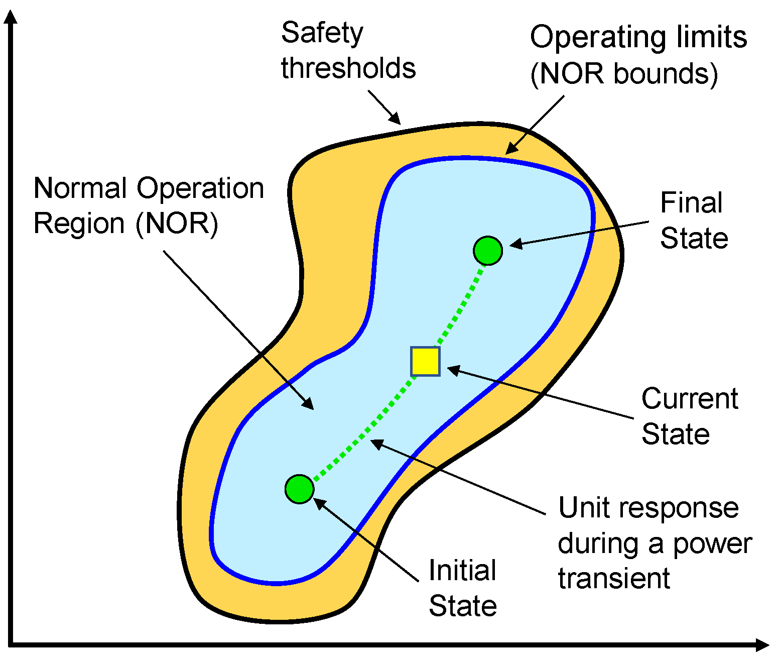
Figure 2.
Tentative solutions to account for both explicit and implicit constraints into the optimization algorithm.
Figure 2.
Tentative solutions to account for both explicit and implicit constraints into the optimization algorithm.
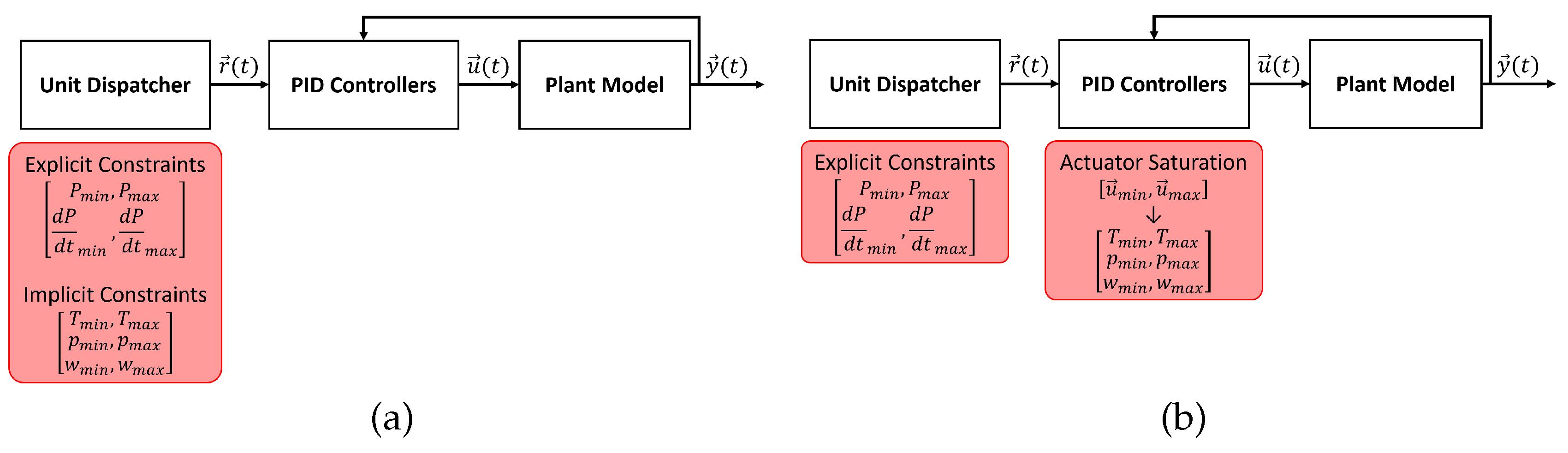
Figure 3.
Proposed scheme for efficiently addressing both explicit and implicit constraints.
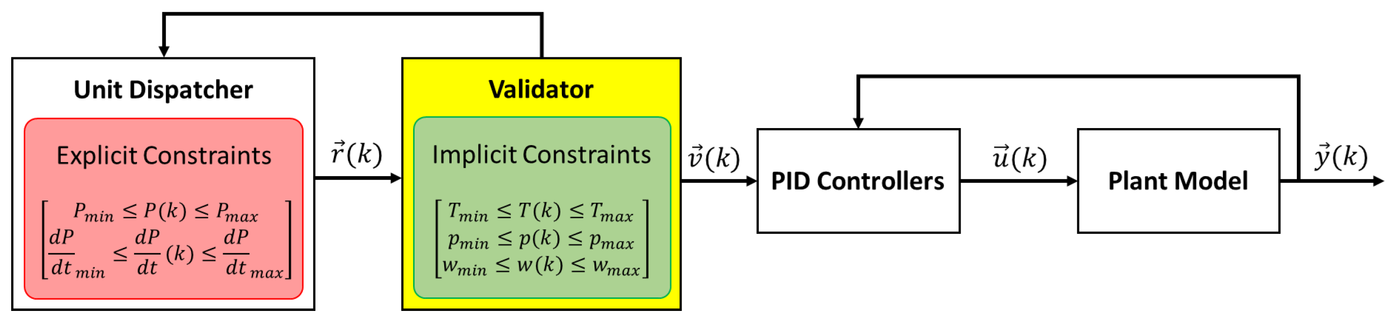
Figure 4.
Graphical representation of the feedback system formed by the Unit Dispatcher and the Validator. The limits on process variables are translated into constraints on production variables and returned to the Unit Dispatcher.
Figure 4.
Graphical representation of the feedback system formed by the Unit Dispatcher and the Validator. The limits on process variables are translated into constraints on production variables and returned to the Unit Dispatcher.
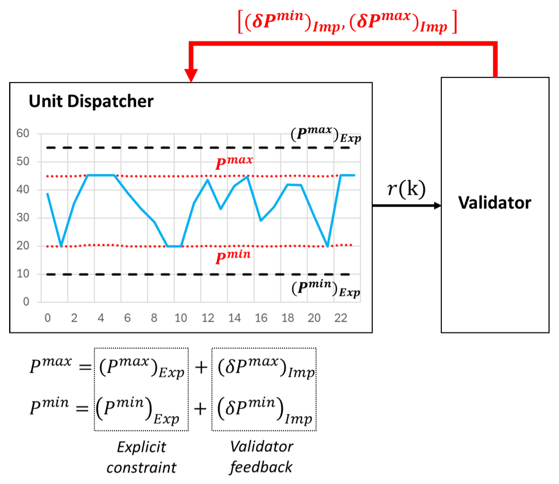
Figure 5.
Workflow of the Framework for Optimization of ResourCes and Economics ecosystem (FORCE) [19]. FARM serves as the bridge between high-fidelity and low-fidelity description of the IES unit.
Figure 5.
Workflow of the Framework for Optimization of ResourCes and Economics ecosystem (FORCE) [19]. FARM serves as the bridge between high-fidelity and low-fidelity description of the IES unit.
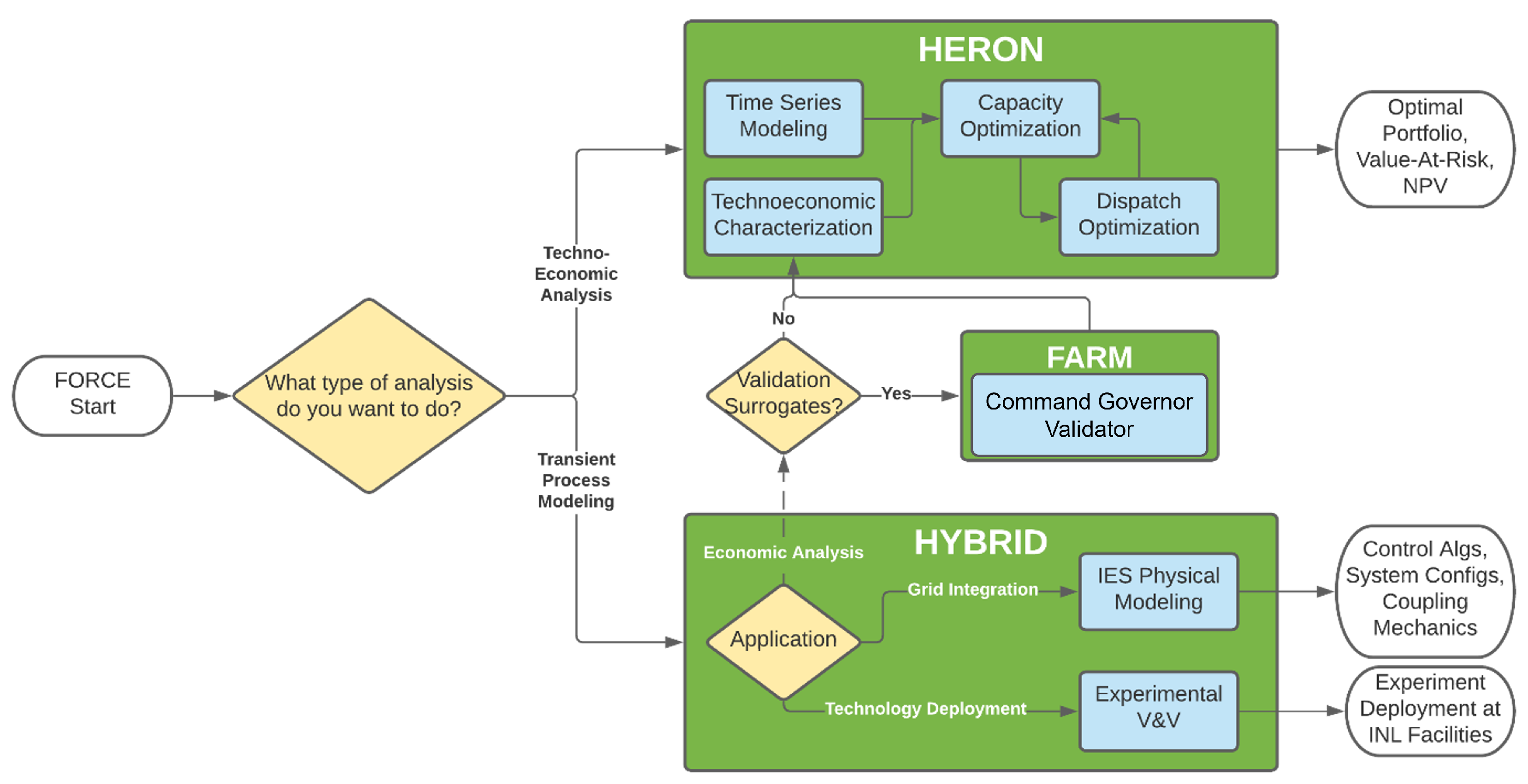
Figure 6.
Detailed view of the FARM-based workflow.
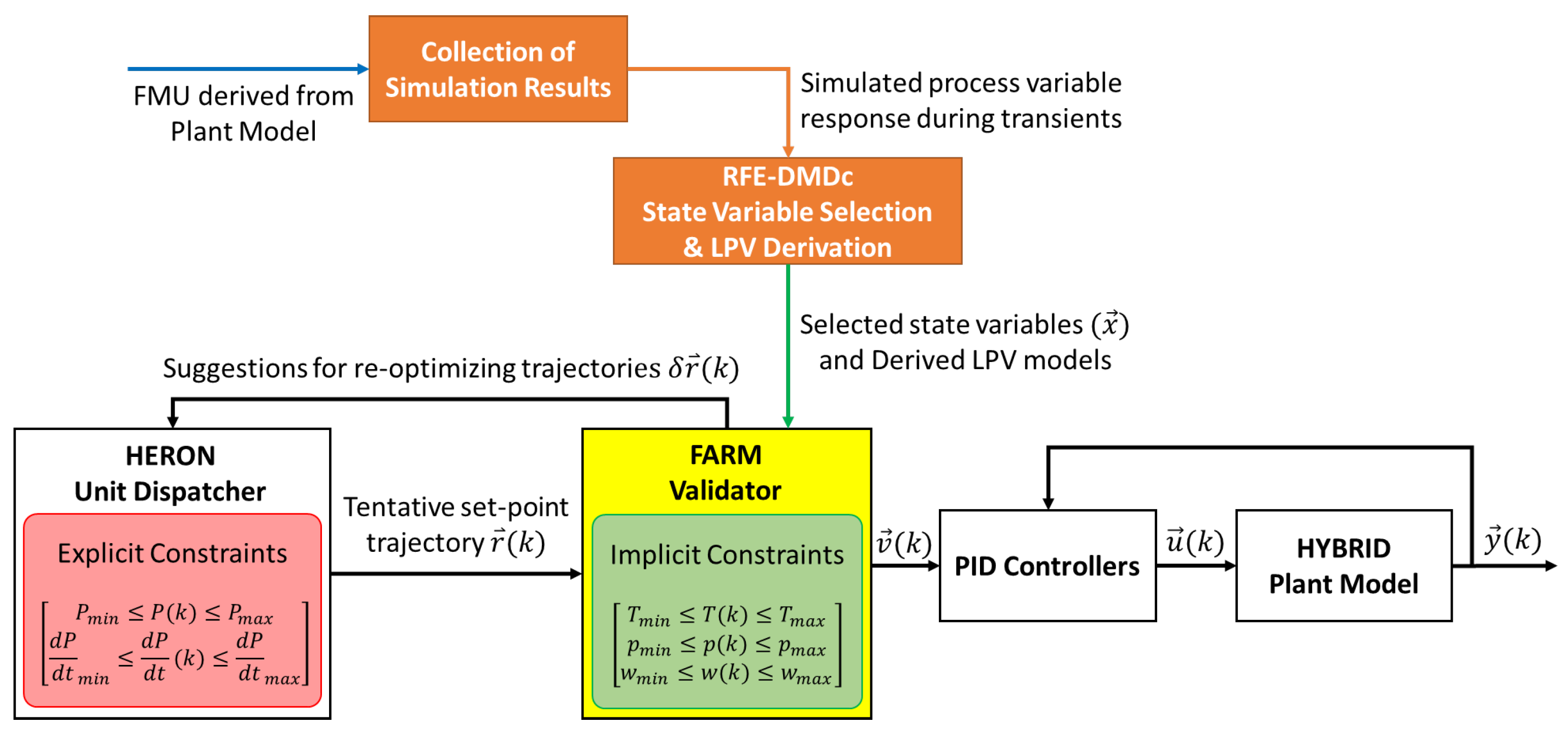
Figure 7.
Graphical representation of the Convex Hull containing 2,888 points.
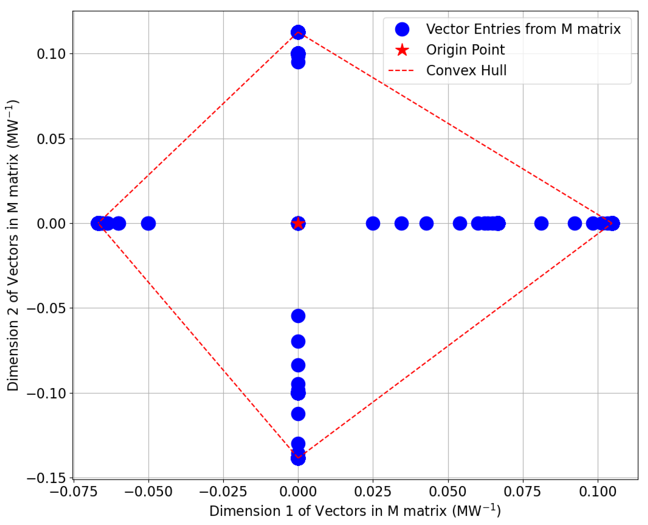
Figure 8.
Comparison of the constrained optimization problem defining the same MOAS. Original MOAS defined by 2,888 constraints and the sub-optimal solution (a), final MOAS defined by 4 non-redundant constraints calculated by the Convex Hull method and the optimal solution (b).
Figure 8.
Comparison of the constrained optimization problem defining the same MOAS. Original MOAS defined by 2,888 constraints and the sub-optimal solution (a), final MOAS defined by 4 non-redundant constraints calculated by the Convex Hull method and the optimal solution (b).
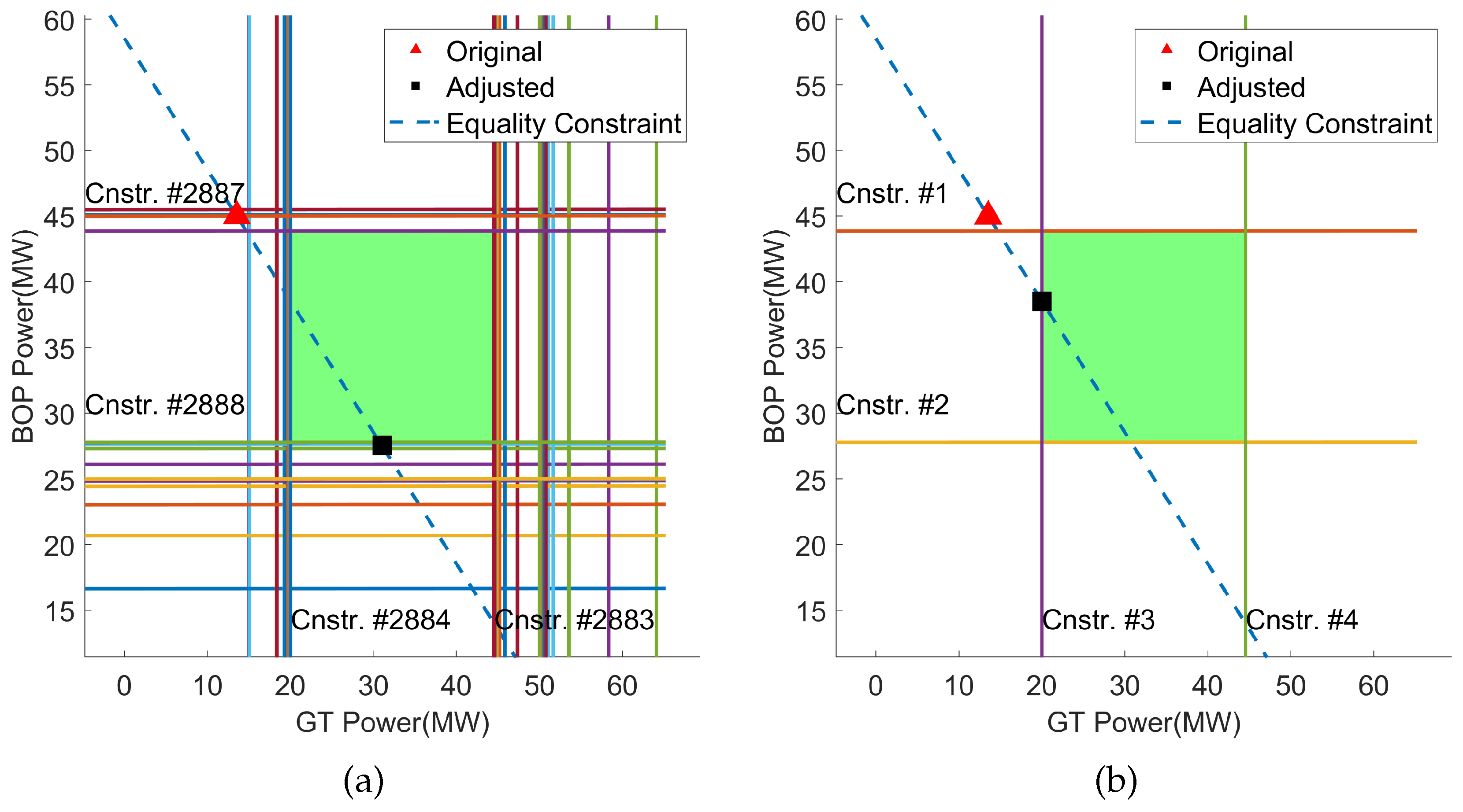
Figure 9.
Simplified representation of interacting subsystems. The process variables for subsystems A and B as well as the state variables of the coupled system are outlined.
Figure 9.
Simplified representation of interacting subsystems. The process variables for subsystems A and B as well as the state variables of the coupled system are outlined.
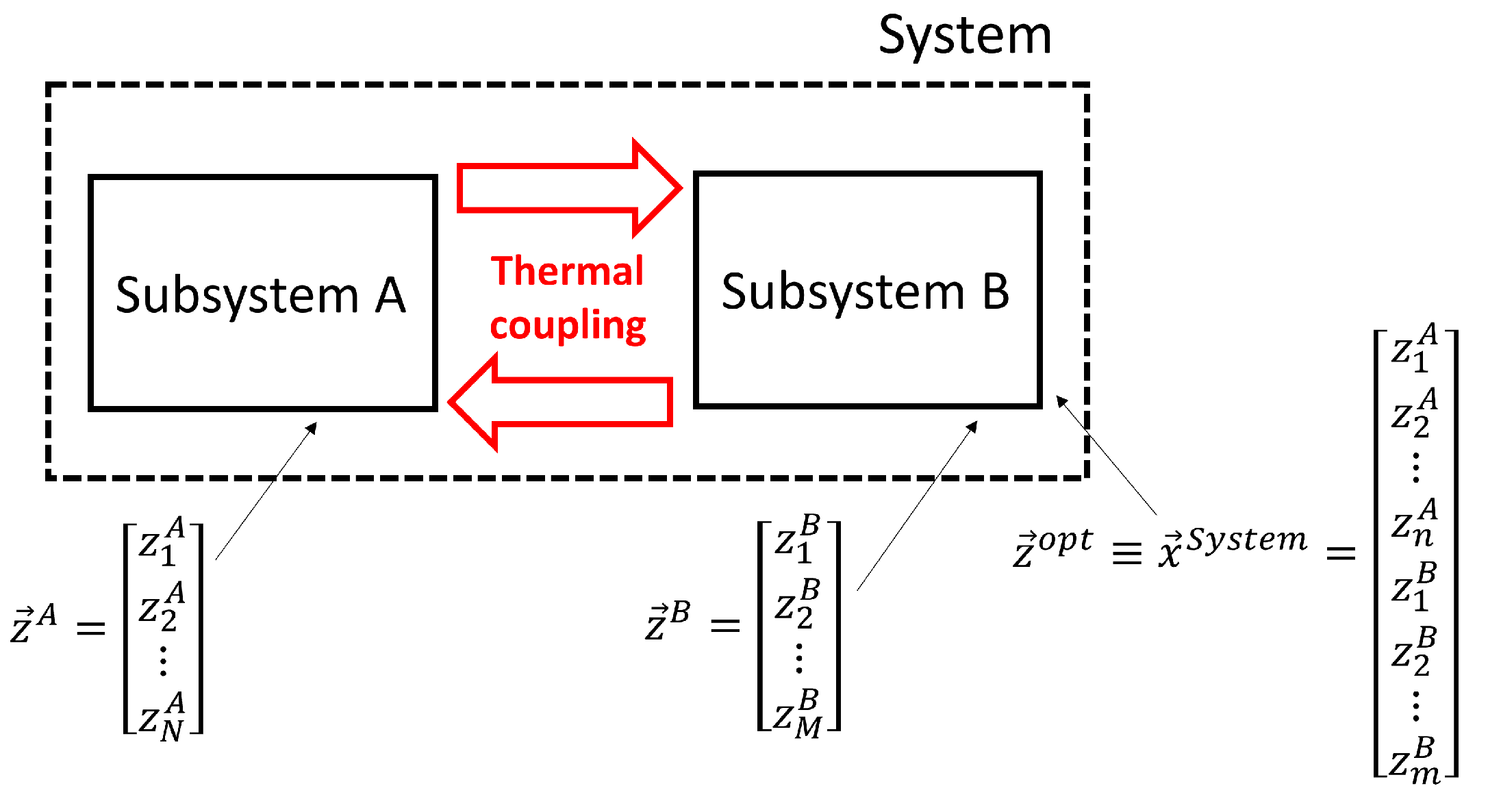
Figure 10.
A graphical representation of the IES unit selected as a test-case. The thermal coupling between subsystems is outlined [45].
Figure 10.
A graphical representation of the IES unit selected as a test-case. The thermal coupling between subsystems is outlined [45].
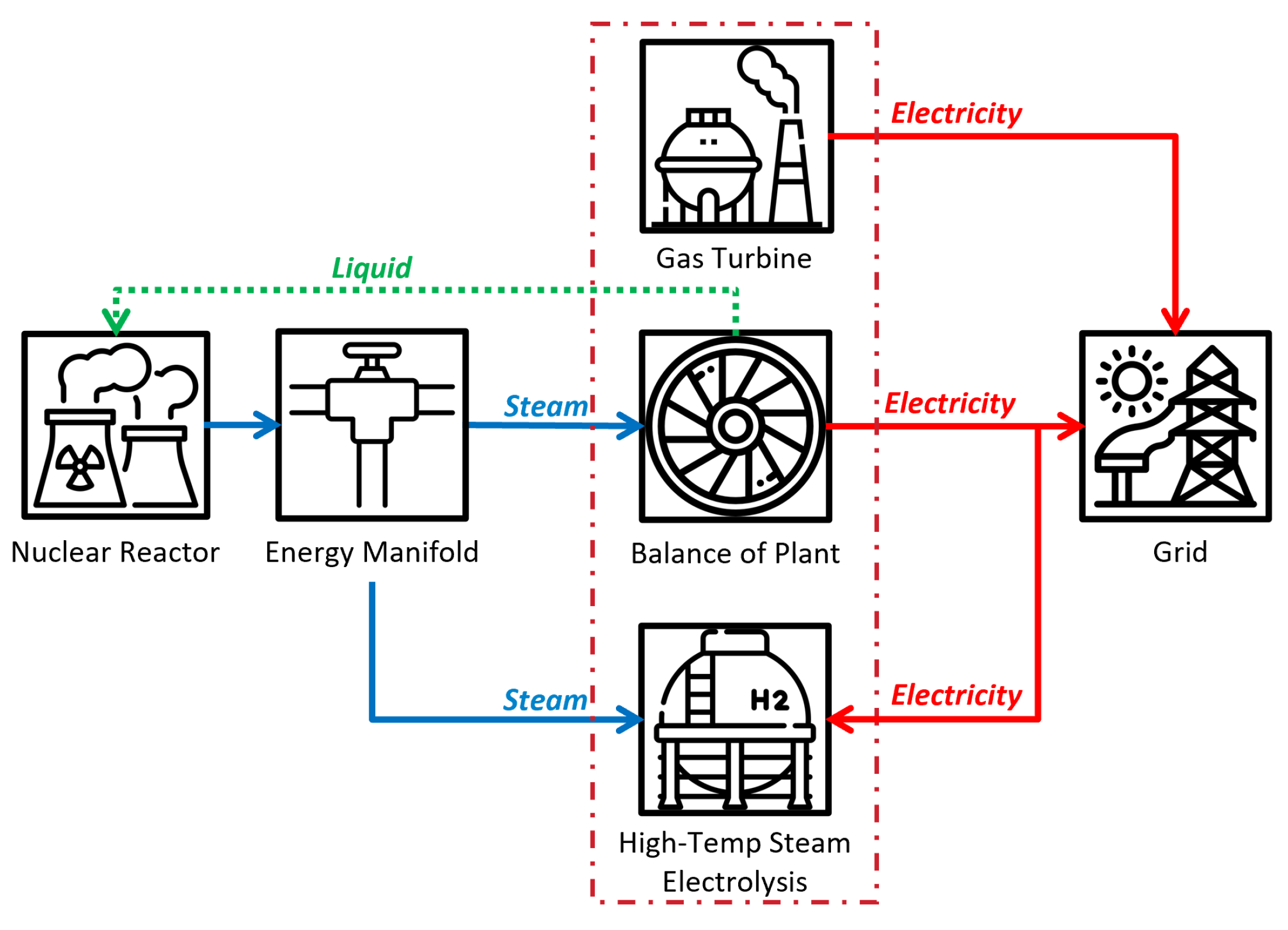
Figure 11.
Graphical user interface of the Dymola GT model [22].
Figure 11.
Graphical user interface of the Dymola GT model [22].
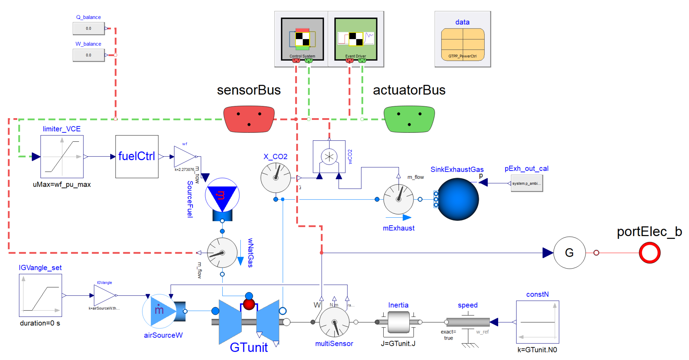
Figure 12.
Graphical user interface of the Dymola BOP model [22].
Figure 12.
Graphical user interface of the Dymola BOP model [22].
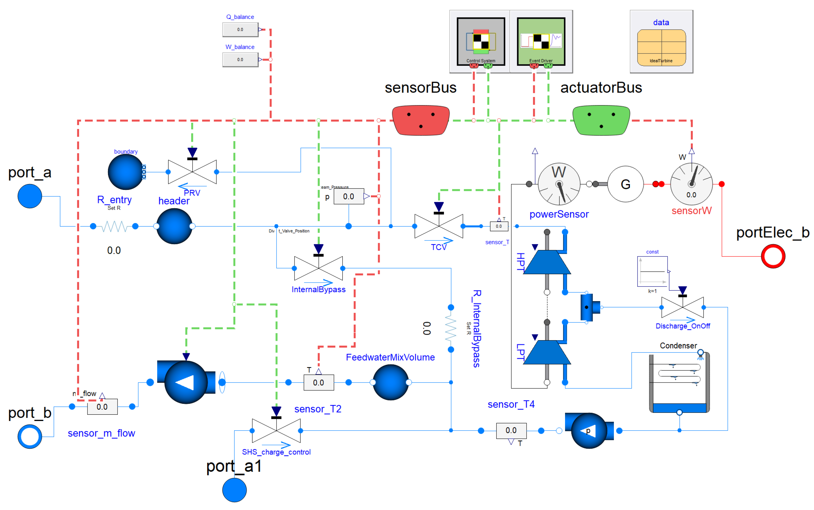
Figure 13.
Graphical user interface of the Dymola HTSE model [22].
Figure 13.
Graphical user interface of the Dymola HTSE model [22].
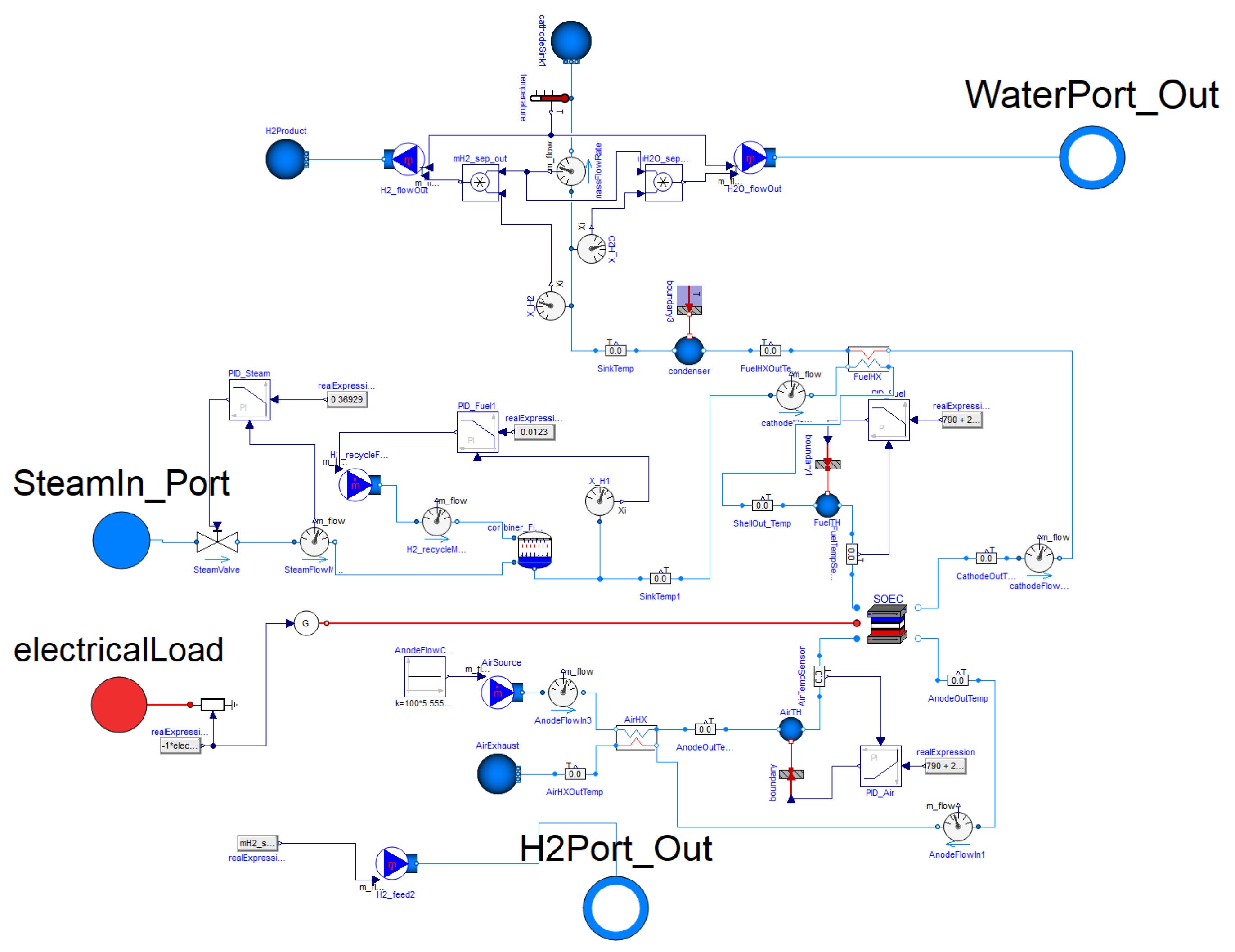
Figure 14.
Representation of the shifted, square-wave shaped set-point trajectories supplied to BOP, GT and HTSE.
Figure 14.
Representation of the shifted, square-wave shaped set-point trajectories supplied to BOP, GT and HTSE.
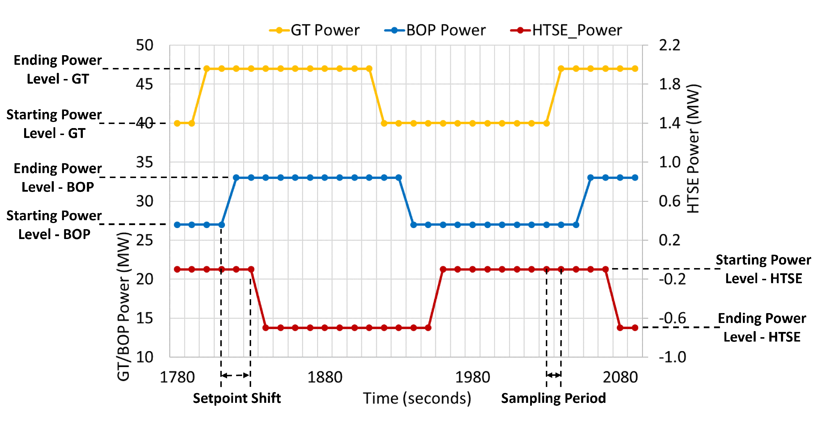
Figure 15.
Validation of the state variable selection. The comparison between the predicted and the expected responses of output variables (top two rows) and selected state variables (bottom row) is shown.
Figure 15.
Validation of the state variable selection. The comparison between the predicted and the expected responses of output variables (top two rows) and selected state variables (bottom row) is shown.
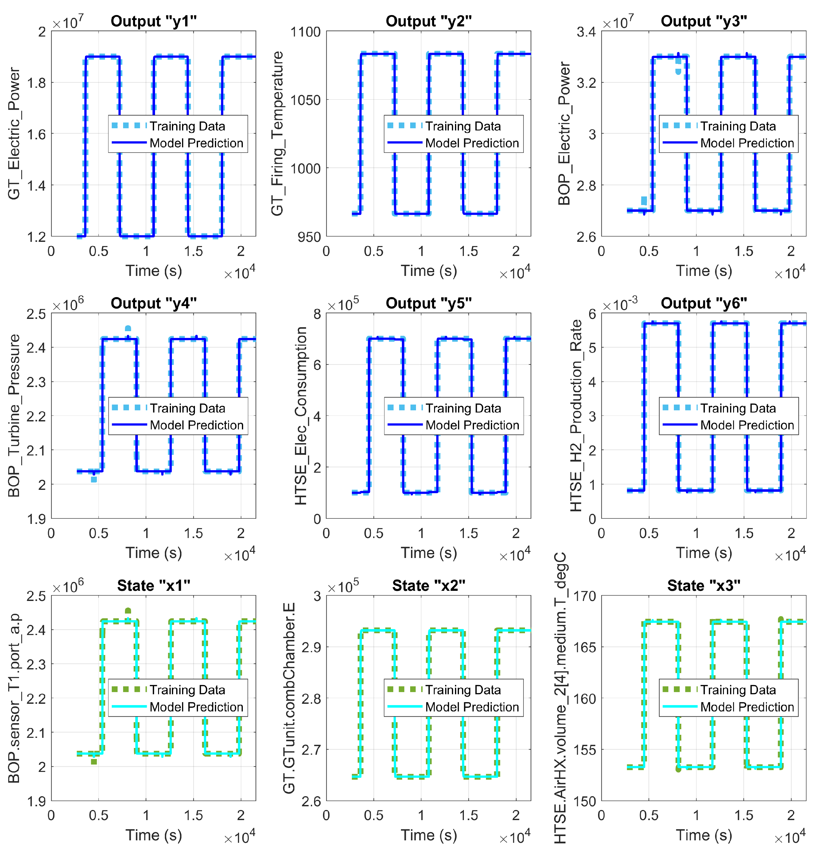
Figure 16.
Graphical representation of using an LPV model to solve the unit dispatch problem. In this simplified illustration, a scalar scheduling parameter is used.
Figure 16.
Graphical representation of using an LPV model to solve the unit dispatch problem. In this simplified illustration, a scalar scheduling parameter is used.
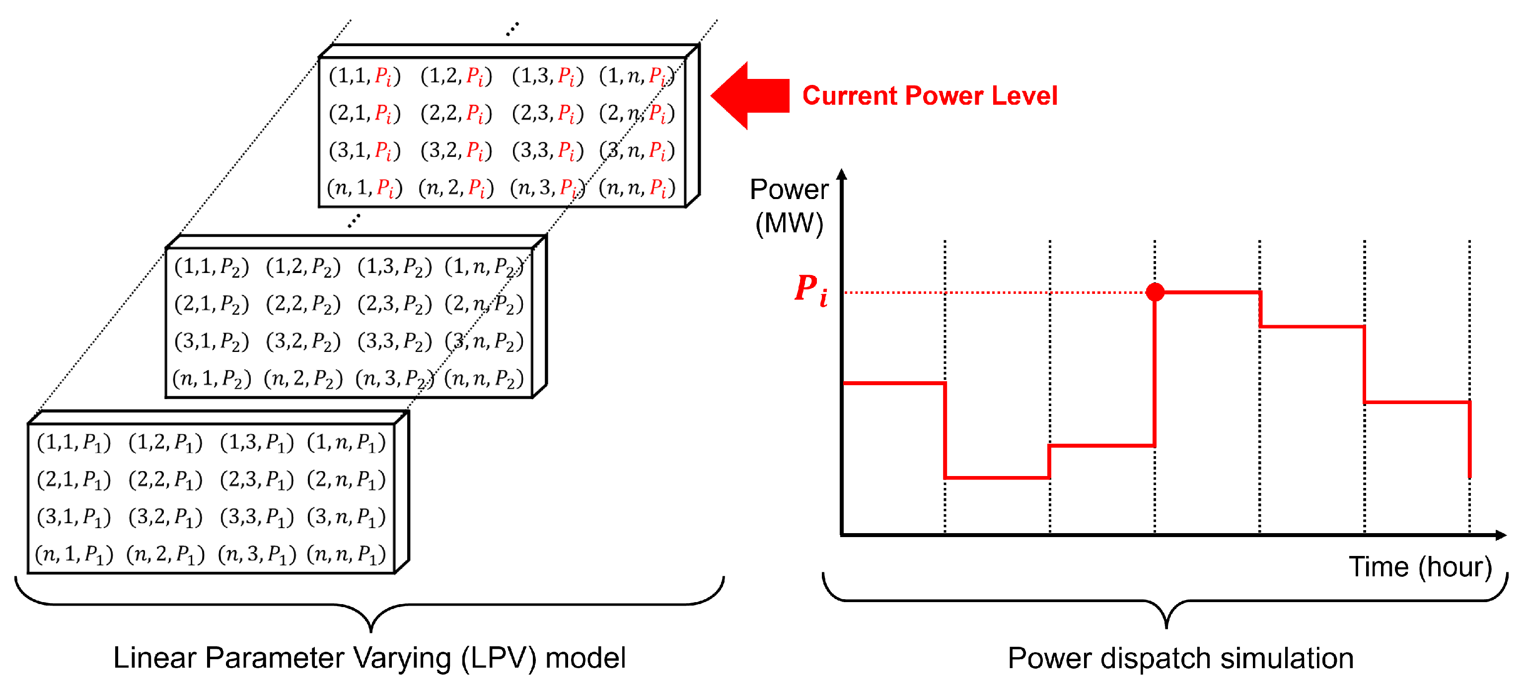
Figure 17.
Solution of Unit Dispatch Problem 1 (time-varying GT generation cost) calculated by HERON-FARM scheme.
Figure 17.
Solution of Unit Dispatch Problem 1 (time-varying GT generation cost) calculated by HERON-FARM scheme.
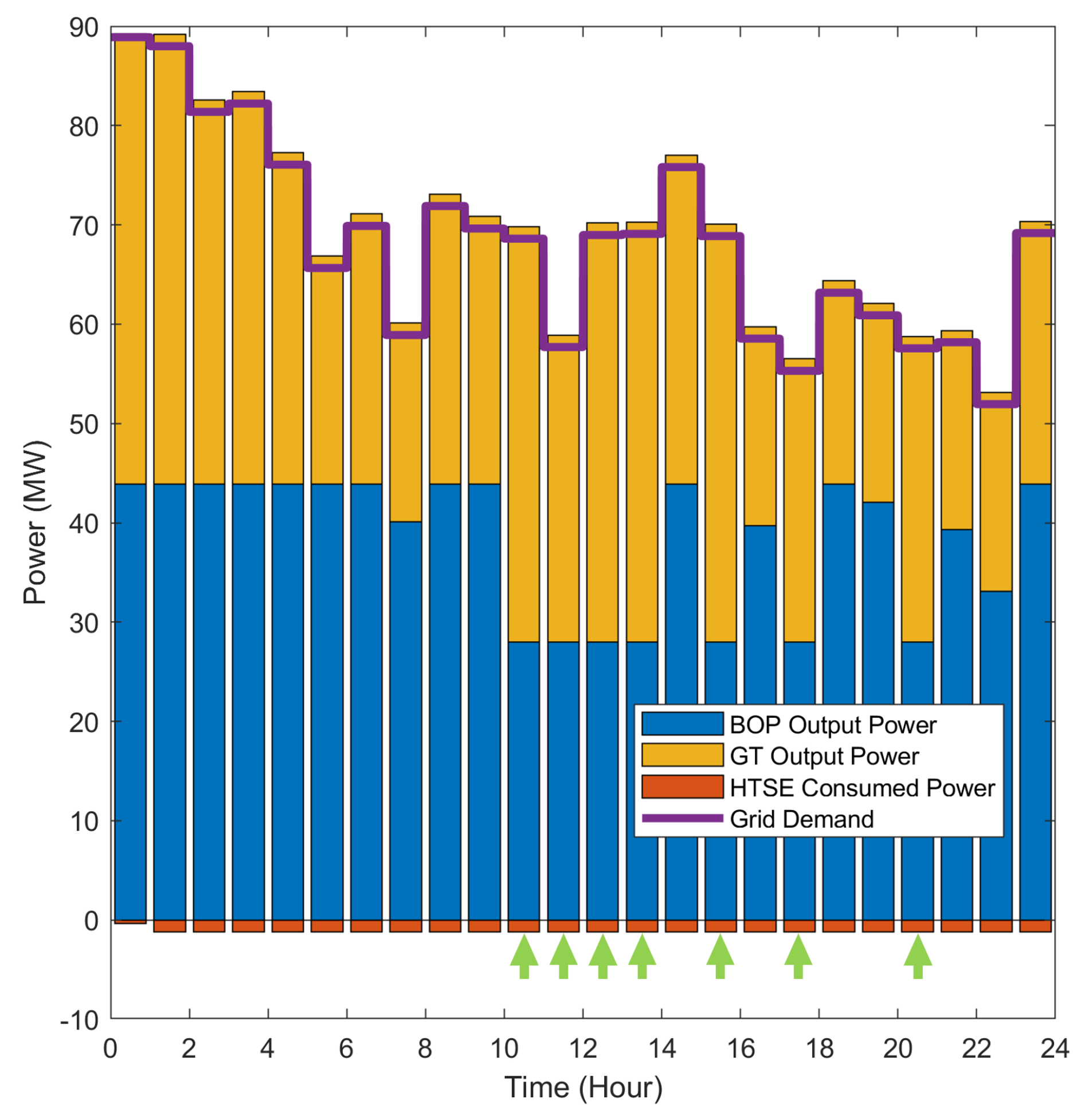
Figure 18.
Trajectories for BOP and GT power generation costs throughout the unit dispatch period.
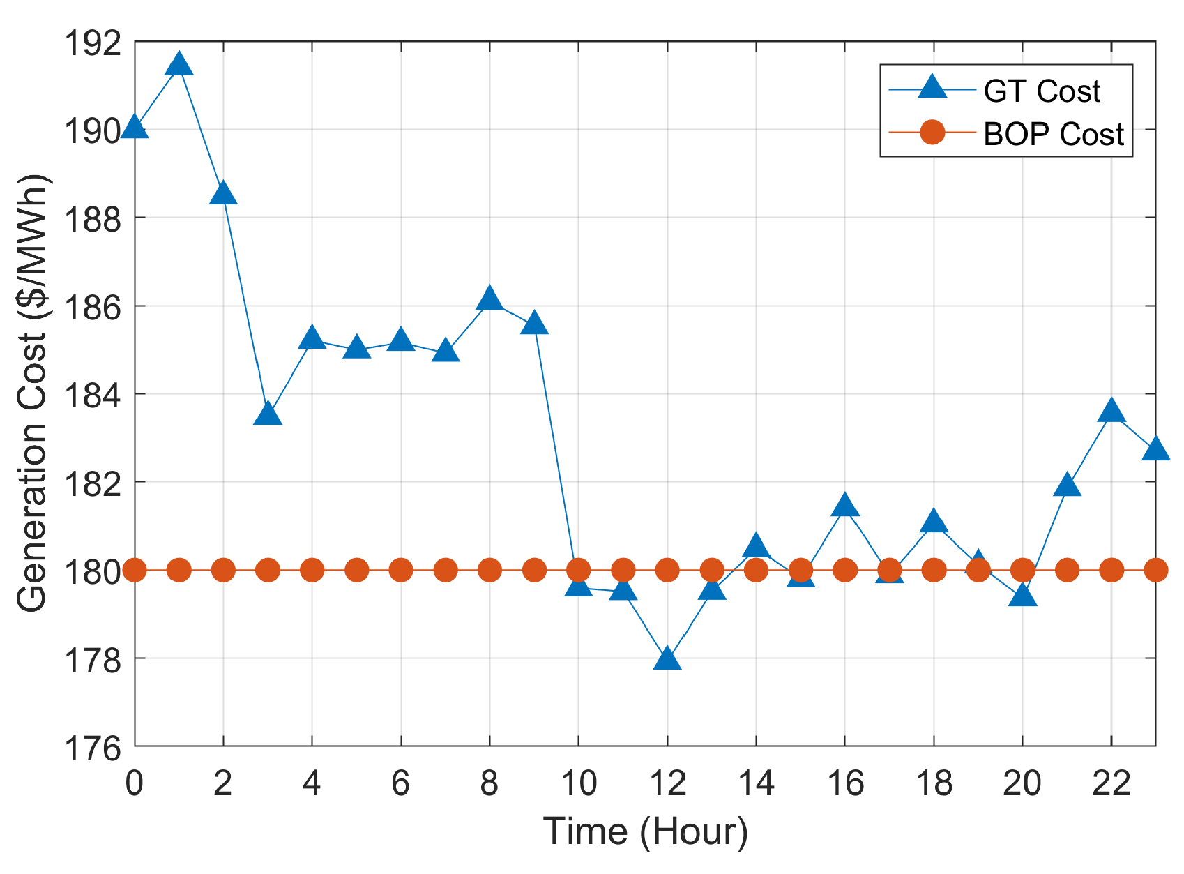
Figure 19.
Responses of output variables for Unit Dispatch Problem 1.
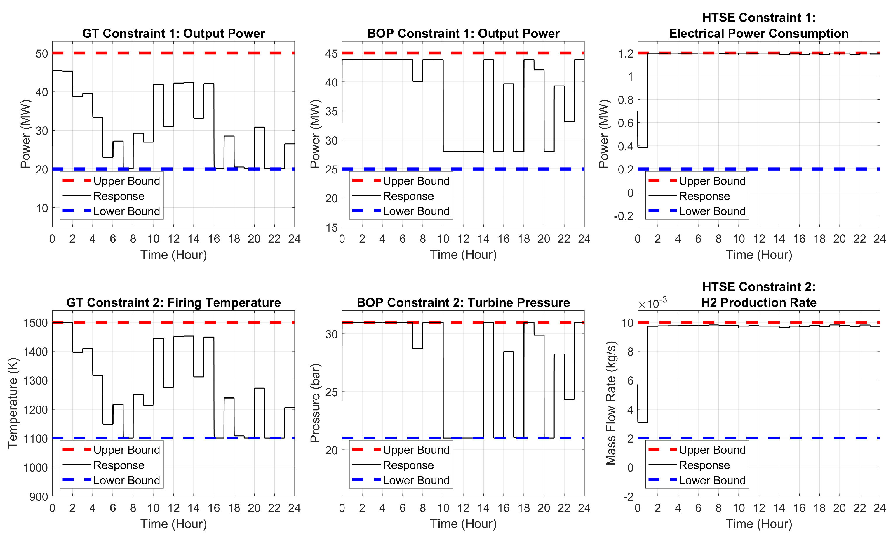
Figure 20.
Iterative feedback between FARM and HERON for Unit Dispatch Problem 1.
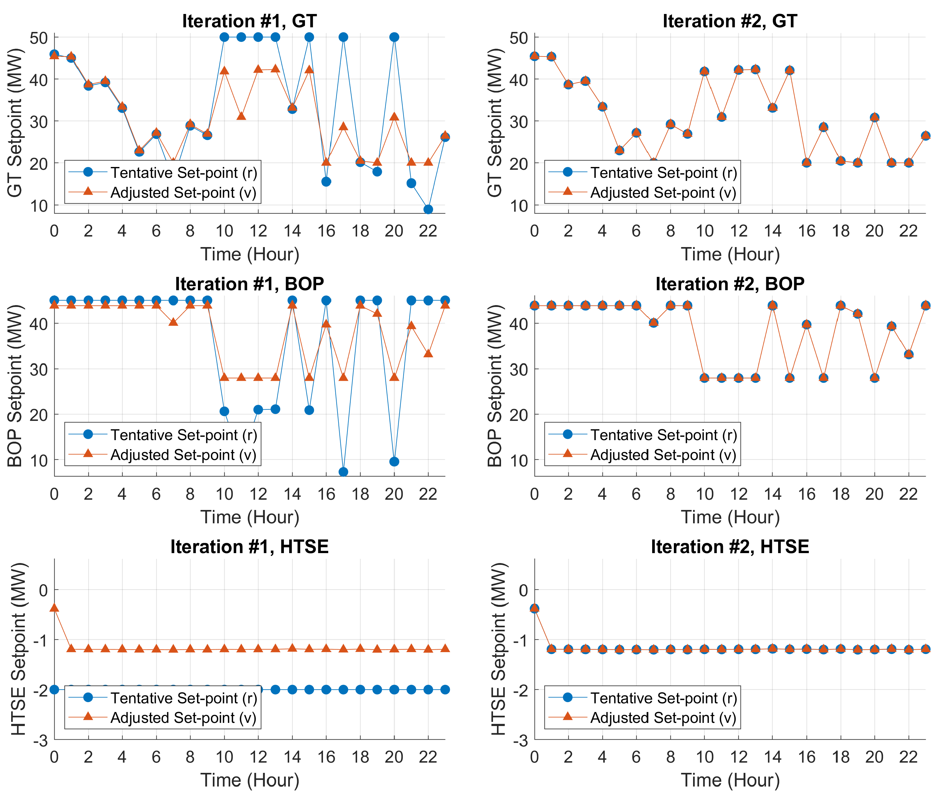
Figure 21.
Hydrogen sales price trajectory throughout the unit dispatch period.
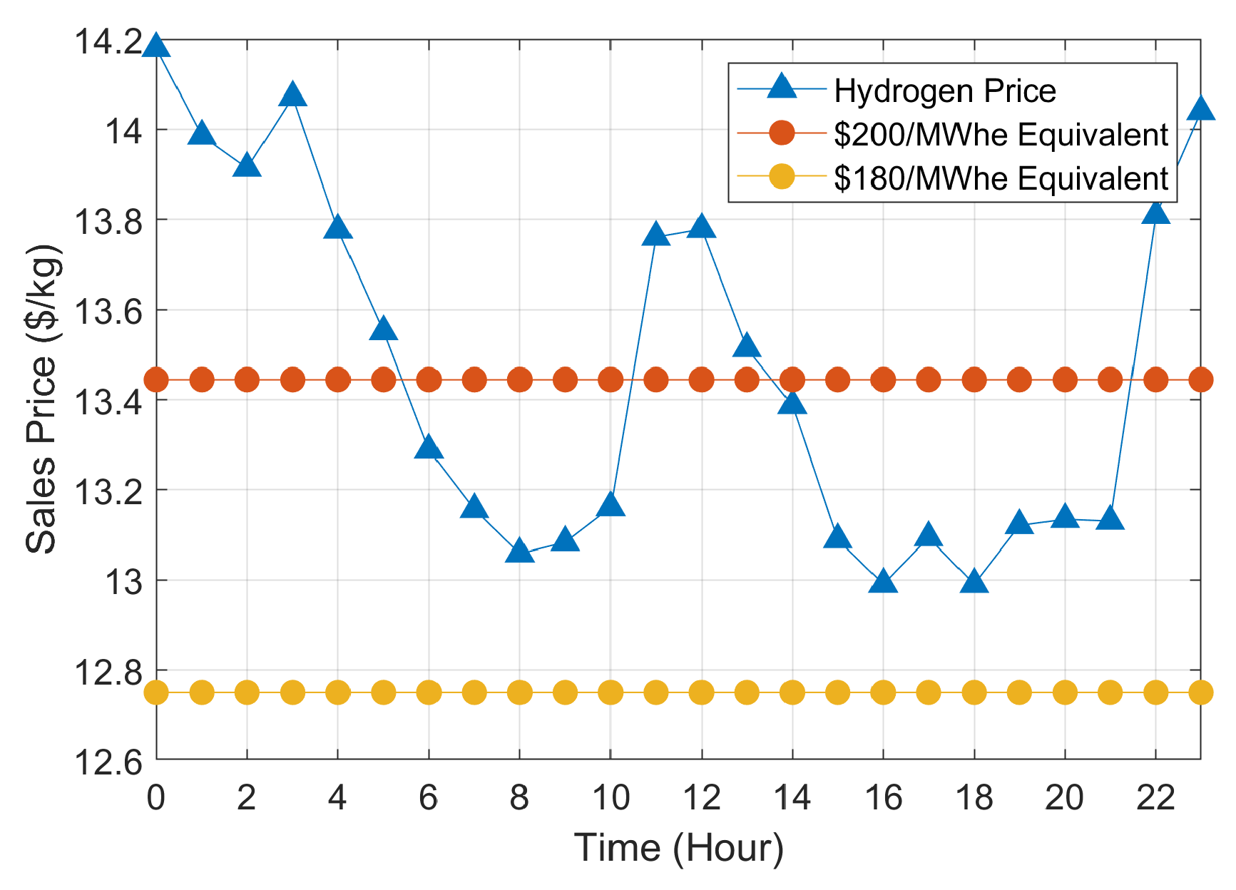
Figure 22.
Solution of the Unit Dispatch Problem 2 (time-varying hydrogen sales price) calculated by HERON-FARM scheme.
Figure 22.
Solution of the Unit Dispatch Problem 2 (time-varying hydrogen sales price) calculated by HERON-FARM scheme.
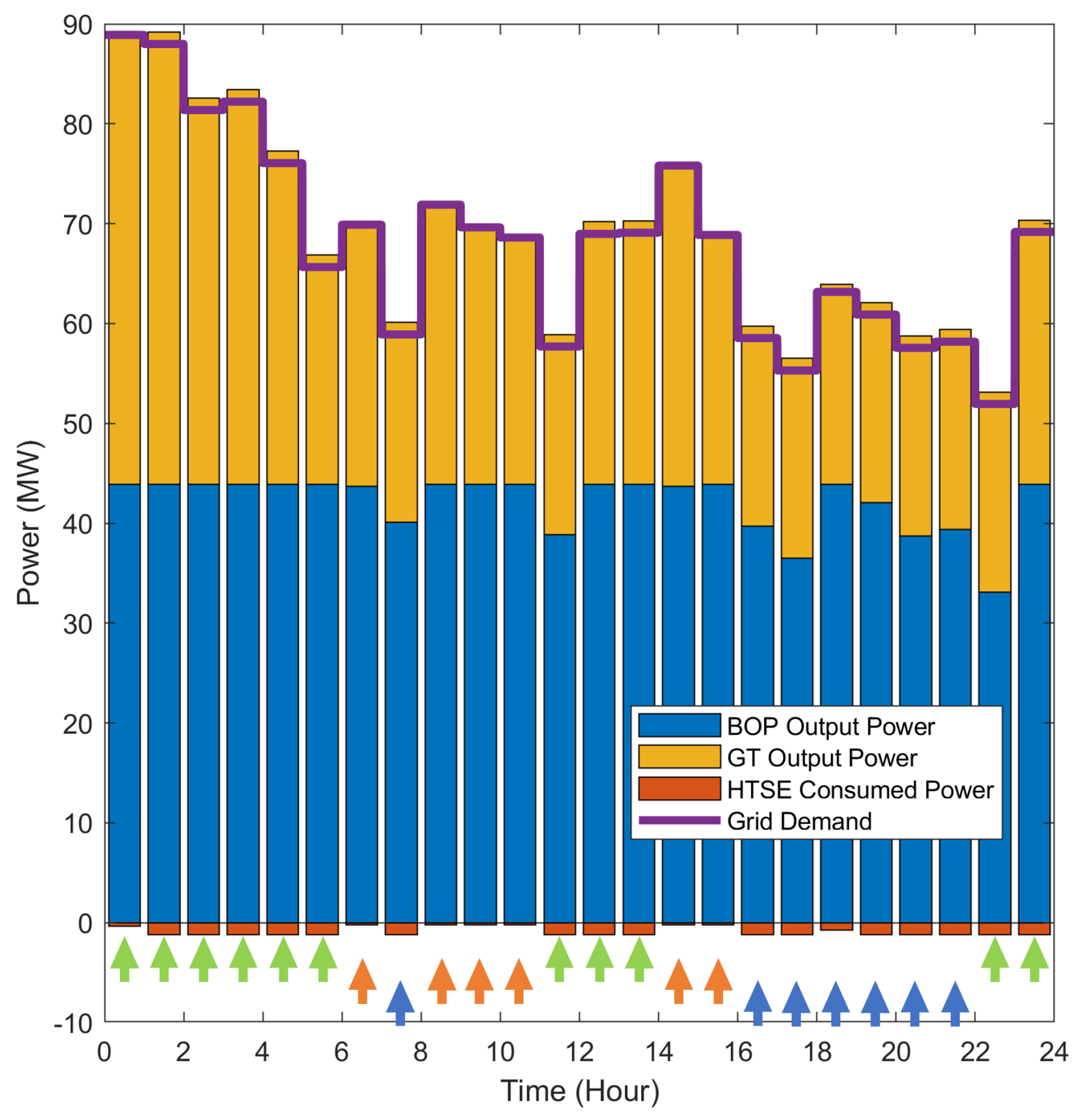
Figure 23.
Efficiency of the HERON-FARM optimization scheme. The computational costs associated with different scheme configurations (with and without FARM validator and for various sample times) (a) and the contributions for a specific case () (b) are shown.
Figure 23.
Efficiency of the HERON-FARM optimization scheme. The computational costs associated with different scheme configurations (with and without FARM validator and for various sample times) (a) and the contributions for a specific case () (b) are shown.

Figure 24.
Dynamic Spider Chart displaying the NOR corresponding to Unit Dispatch Problem 1 at time .
Figure 24.
Dynamic Spider Chart displaying the NOR corresponding to Unit Dispatch Problem 1 at time .
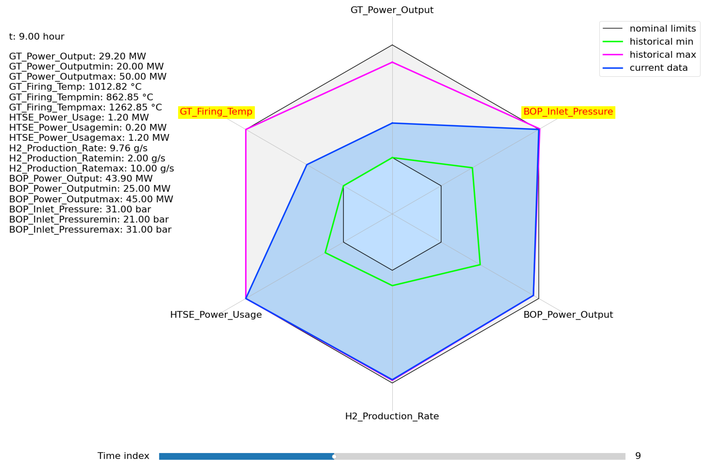
Figure 25.
Phase Space Diagram displaying the NOR corresponding to Unit Dispatch Problem 1 at time .
Figure 25.
Phase Space Diagram displaying the NOR corresponding to Unit Dispatch Problem 1 at time .
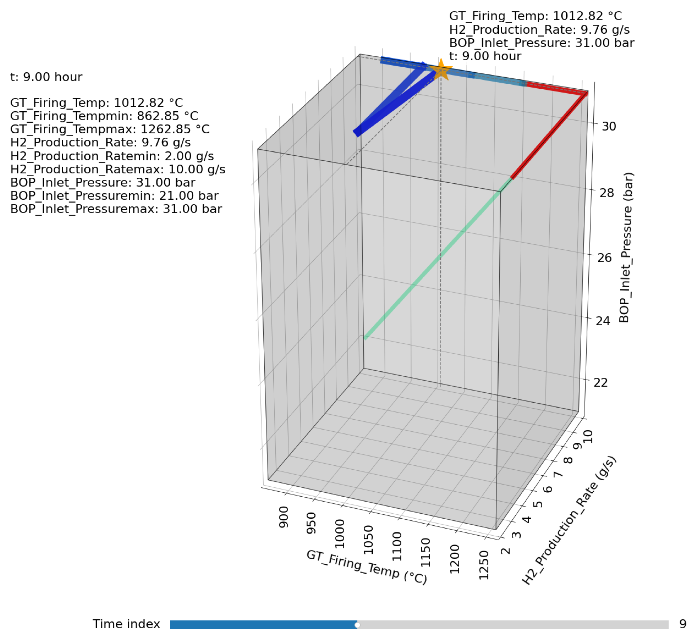
Figure 26.
Representation of the Admissible Region calculated by the CG algorithm during the solution of Unit Dispatch Problem 1 at time (first iteration).
Figure 26.
Representation of the Admissible Region calculated by the CG algorithm during the solution of Unit Dispatch Problem 1 at time (first iteration).
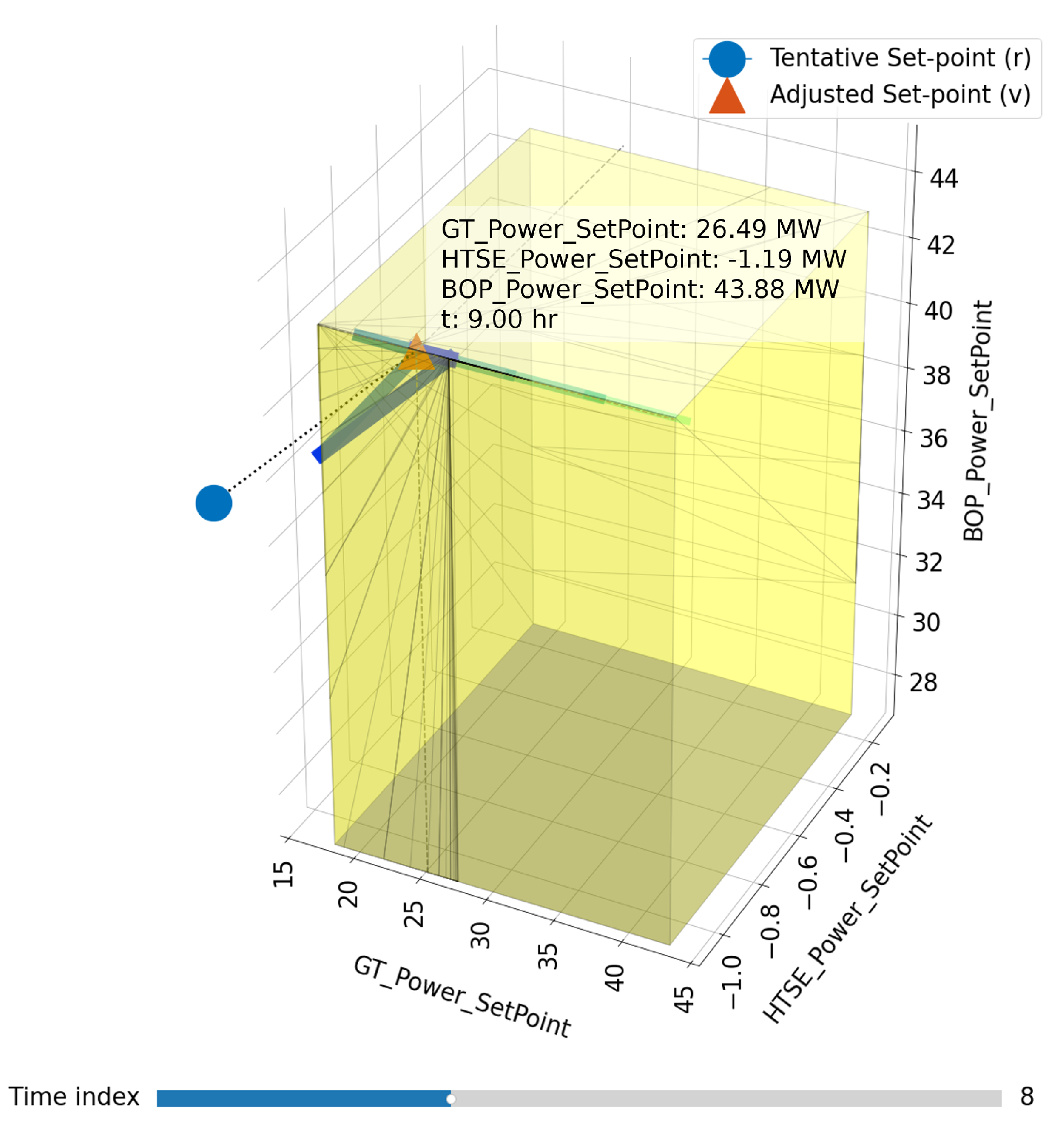

Table 1.
List of input and constrained output variables for each subsystem. The adopted values for the upper and lower bounds are reported.
Table 1.
List of input and constrained output variables for each subsystem. The adopted values for the upper and lower bounds are reported.
| Subsystem | Input (v) | Outputs () | Lower | Upper |
|---|---|---|---|---|
| Bounds | Bounds | |||
| GT | Power set- | Electrical power output () | 20.0 MW | 50.0 MW |
| point () | Firing temperature () | 1100 K | 1500 K | |
| BOP | Power set- | Electrical power output () | 25.0 MW | 45.0 MW |
| point () | Turbine inlet pressure () | 21.0 bar | 31.0 bar | |
| HTSE | Power set- | Electrical power consumption () | 0.2 MW | 1.2 MW |
| point () | Hydrogen production rate () | 2.0 g/s | 10.0 g/s |
Table 2.
Starting and ending values of the power set-point trajectories supplied to BOP, GT and HTSE.
Table 2.
Starting and ending values of the power set-point trajectories supplied to BOP, GT and HTSE.
| Subsystem | Starting Power Level (MWe) | Ending Power Level (MWe) |
|---|---|---|
| GT | 19.0 | 26.0 |
| 26.0 | 33.0 | |
| 33.0 | 40.0 | |
| 40.0 | 47.0 | |
| 47.0 | 19.0 | |
| BOP | 27.0 | 33.0 |
| 33.0 | 39.0 | |
| 39.0 | 45.0 | |
| 45.0 | 27.0 | |
| HTSE | -0.11 | -0.71 |
| -0.71 | -1.31 | |
| -1.31 | -0.11 |
1 Negative values indicate power consumption.
Table 3.
List of the state variables selected by the RFE-DMDc algorithm.
| State Variable | Name and Physical Meaning |
|---|---|
| BOP.sensor_T1.port_a.p | |
| (Steam pressure at High Pressure Turbine inlet (Pa)) | |
| GT.GTunit.combChamber.E | |
| (Total gas energy within the Combustion chamber (J)) | |
| HTSE.AirHX.volume_2[4].medium.T_degC | |
| (Air temperature at node 4 of Air Heater exchanger hot side volume (°C)) |
Table 4.
Adopted economic parameters in two unit dispatch problems.
| Parameter | Dispatch Problem 1 | Dispatch Problem 2 |
|---|---|---|
| BOP Generation Cost | $180.0/MWh | $180.0/MWh |
| GT Generation Cost | Time-varying | Constant |
| $177.9 - $191.4/MWh | $200.0/MWh | |
| Hydrogen Sales Price | Constant | Time-varying |
| $14.0/kg | $13.0 - $14.2/kg | |
| ($216.0/MWh of | ($186.9 - $221.2/MWh of | |
| consumed electricity) | consumed electricity) | |
| Electricity Sales Price | $400.0/MWh | $400.0/MWh |
Table 5.
Computational costs for solving Unit Dispatch Problem 1 using different configurations of HERON-FARM scheme. All the reported values for the task duration are expressed in seconds.
Table 5.
Computational costs for solving Unit Dispatch Problem 1 using different configurations of HERON-FARM scheme. All the reported values for the task duration are expressed in seconds.
| Sample Time | LPV Derivation | HERON Dispatcher | FARM Validator |
|---|---|---|---|
| 30.0 | |||
| 60.0 | |||
| 100.0 | |||
| 150.0 | |||
| 225.0 | |||
| 300.0 |
Disclaimer/Publisher’s Note: The statements, opinions and data contained in all publications are solely those of the individual author(s) and contributor(s) and not of MDPI and/or the editor(s). MDPI and/or the editor(s) disclaim responsibility for any injury to people or property resulting from any ideas, methods, instructions or products referred to in the content. |
© 2024 by the authors. Licensee MDPI, Basel, Switzerland. This article is an open access article distributed under the terms and conditions of the Creative Commons Attribution (CC BY) license (http://creativecommons.org/licenses/by/4.0/).
Copyright: This open access article is published under a Creative Commons CC BY 4.0 license, which permit the free download, distribution, and reuse, provided that the author and preprint are cited in any reuse.


