
Submitted:
02 May 2024
Posted:
07 May 2024
You are already at the latest version
Abstract
In this work, we explore the ability to dynamically group the Wind Turbine (WT) of a Wind Farm (WF) based on the behaviour of some of their Supervisory Control And Data Acquisition (SCADA) signals to detect the turbines that exhibit abnormal behaviour. We centre this study on a small WF of five WTs. We use the fact that the same signals from different turbines in the same WF coherently evolve temporally in a time domain, describing very similar waveforms. In this contribution, we use averaged signals from the SCADA system and omit maximums, minimums and standard deviations, focusing mainly on velocities and other slowly varying signals. For the temporal analysis, sliding windows of different temporal durations and overlapings are explored. The capability to automatically identify WTs whose signals differ from the group’s behaviour can alert and program preventive maintenance operations on such WTs before a major breakdown occurs.
Keywords:
Hierarchical Clustering (HC)
; Wind Turbine (WT)
; SCADA Data
; Industrial AI
; Dynamic Clustering (DC)
1. Introduction
The urgent need to transition to more sustainable energy sources directly responds to the challenges imposed by climate change and the growing global energy demand. In this scenario, wind power stands out as a promising alternative, showing remarkable technological development and capacity expansion in recent decades. Thus, it has established itself as one of the primary renewable energy sources, with increasing acceptance by society and strong support from international public policies.
WFs made up of sets of WTs, play an essential role in transforming wind into electrical energy. The efficient management of these parks is critical not only to ensure optimal energy production but also to extend the useful life of the equipment and minimize periods of inactivity. An effective preventive maintenance system, which proactively identifies potential failures before they become major problems, is key to achieving these goals [1,2,3]
The present research proposes dynamically applying the Hierarchical Cluster (HC) method to SCADA data to understand and manage turbines’ operational behaviour better. This approach is novel because it applies clustering based on the shape of signals considered in consecutive time windows.
Groupings of WT sets with similar characteristics in the WF will allow the WF operators to understand their operation and improve their management and maintenance. Specifically, in this work, we explore the ability to group WTs according to criteria of similarity of specific signals since this would allow us to compare the subsystems of the machines that generate them and behave similarly to detect possible irregularities prematurely. This can be of particular relevance when monitoring, for example, temperatures at critical points of the WT. In the context of WTs, this task presents specific difficulties since the behaviour of WTs is highly non-linear and varies enormously over time. The WTs are subject to important behaviour changes due to wind fluctuation and other meteorological changes. Consequently, the variations of the shapes of the collected signals over time, or equivalently, the characteristics that represent them, also vary enormously.
As observed and proposed in [4,5], a detailed analysis of the variability and continuity of the collected signals and clustering WTs appropriately will facilitate the early detection of anomalies and the planning of maintenance interventions [6].
In the literature, clustering techniques have been used in the context of WTs in different ways, for instance, in [7,8]. Liu et al.’s (2014) article [9] explores the application of WT clustering methods to improve short-term wind power forecasts. These authors develop and validate different clustering techniques to categorize turbines based on similar performance characteristics, enabling more accurate prediction models. This research proposes using clustering to optimize energy management strategies, resulting in more accurate and efficient power generation predictions. The article [10] addresses the development of a dynamic cluster equivalent model for WTs based on the use of spanning trees. This approach allows the clustering of WTs dynamically to improve the efficiency and representativeness of WF simulation models. Such an approach uses spanning tree techniques to identify and represent the most critical connections between turbines, thus facilitating the creation of simplified yet effective equivalent models. This methodology offers a significant advancement in modelling the collective behaviour of WTs, contributing to improving WF planning and operation. The article [4] presents a method for diagnosing and warning of faults in WTs using cluster analysis and a modified version of the Adaptive Neuro-Fuzzy Inference System (ANFIS). The article [11] presents an advanced methodology for early fault detection in WTs, combining operational condition clustering with optimised deep belief network modelling. This approach segments WT operations into different sub-conditions, facilitating more effective detection of possible anomalies and improving fault detection accuracy by effectively handling the WTs’ nonlinear and heterogeneous operational data. The article [5] explores a new strategy for fault detection in WTs through SCADA data clustering. This methodology groups WTs based on similarities in operational data to enhance fault detection and diagnosis, enhancing detection and diagnosis through comparative analysis. Finally, advanced data visualization techniques are implemented to represent the information and facilitate its graphic interpretation. This study seeks to provide a clear and detailed understanding of the dynamics within the WF by using scatter plots, time plots and other graphical tools. The HC process is then applied to identify groupings of data that will share similar properties, revealing meaningful patterns that can inform maintenance and operation decisions [9,10]. This approach improves WFs’ operational performance and provides a replicable and scalable methodology for data analysis in other industrial applications, expanding companies’ ability to adapt to technological and market changes.
In the present work, we focus on the problem of dynamic clustering [12] based on the shape of specific signals. We analyze a signal of all WT in a WF fragment-by-fragment in time windows we call frames, which, in the first experiments, initially lasted around one day. We obtain the clustering of the signals of each WT in every frame. Clustering considers the shapes of those signals in a temporal frame; we obtain clustering updated with every new frame.
The detailed methodology first involves a comprehensive review and selection of the most impactful variables, such as air temperature, relative humidity, wind speed, and generated power. The next step involves a meticulous data cleaning process, where the inputs are selected and filtered to remove outliers or erroneous values. This task is crucial to maintaining the integrity of the analytical model [11,13] but is very common, so we do not focus on it very much. The database employed for this work contains SCADA signals that provide data every 5 minutes, so they collected 288 points daily. More relevant in our approach is that to compact the information, we use the Discrete Cosine Transform (DCT), and we consider only the first coefficients that we organize in vectors of features to represent the signals frame-to-frame. The experiments reveal that a few coefficients (3 to 5) already synthesize the information very effectively.
We use the representative vectors of each signal to calculate the distances (we use the Euclidean distance) between each pair of signals. Then we build a binary, agglomerative, HC tree from those distances [14]. In this step, the objects (signals) are linked in pairs according to proximity, building a series of nested clusters, where the most similar elements are grouped first, and differences are incorporated as one descends the hierarchy. In agglomerative clustering, each element starts as an independent cluster and progressively merges into larger clusters based on similarity. This hierarchical tree (HT) provides an intuitive view of data structure, allowing exploration of different levels of detail in organizing elements, which is helpful in classification and pattern exploration in complex datasets because one can cut the HT to form the clusters at any particular point independently of a preestablished number of clusters [15]. Finally, we develop a way to name the clusters so that the signals with the most similarity appear in the first cluster, and as they differ more, they appear in higher clusters. This nomenclature facilitates, at least in a small WF, the monitoring of the temporal evolution of the clusters.
This work will be organized into a Materials and Methods (section 2) where we provide detailed descriptions of the following contents: the data used, the shape parameterization based on the Discrete Cosine Transform (DCT) coefficients, a description of the hierarchical clustering employed, and the protocol to name the clusters that permits to follow the temporal evolution of clusters. Then, section 3, Results, explains the interpretation of the dynamical clustering graphs and contains two experiments. The first is a study of the wind speeds recorded in the WTs’ nacelles through these clustering techniques. The second is a comparative study of applying this technique to two control variables commonly used for wt prognosis, such as the rotation speed of the generator shaft and the temperature of the oil in the gearbox. Finally, the main Conclusions are summarized in Section 4.
2. Materials and Methods
2.1. Data Used
The present study thoroughly analyzes SCADA records of five 2.5 MW Fuhrläender FL2500 wind turbines for three years and a sampling frequency of 5 minutes. The system has IEC 61400-25 as its standard communication protocol for transmitting data from the wind turbines and storing it in a MySQL database. This database includes 312 analog variables from 78 different sensors. Thus, the status of various essential components, such as the transmission, generator, and converter, among many others, can be known. The data are extracted from the open-access database available at https://github.com/alecuba16/fuhrlander, and it is described in [16].
2.2. Shape Parameterization trough the DCT
In this work, we will exploit the DCT as a tool for parameterizing relatively long signals into a few parameters to compress their information. Unlike other transforms, such as the Fourier Transform, which yields complex-valued coefficients, DCT produces real-valued ones, simplifying signal processing.
To present it, let us consider the set of N points , and their N DCT (of type-II) transformed coefficients . The forward and backward expressions take the form:
and,
Where for and for .
As it is well known, one of DCT’s key features is its ability to concentrate most of the signal energy into a few coefficients. Thus, a relatively small number of coefficients can capture much of the signal’s information, making it an efficient representation for compression purposes. In many applications, such as image and video compression, DCT is applied to small blocks of the signal rather than the entire signal. This block-based processing allows for parallelization and efficient implementation. DCT, like other discrete transforms, also has fast algorithms that are being computed very efficiently. Additionally, DCT has an inverse transform that reconstructs the original signal from its DCT coefficients. This property is essential for applications where compression is used, as it facilitates decompression to retrieve the original signal.
To concentrate the shape characteristics of the time series of length N in a few parameters, we will take advantage of the compaction properties presented by the DCT in the first coefficients of the transform. So, we will work in the transformed domain, characterizing the N points of the signals by the L first transformed coefficients of their DCTs, where L will be much smaller than N. It is interesting to check the reconstruction capacity of only the L=2, 4, or 6 DCT coefficients to reconstruct a sequence of 128 points from the following reconstruction formula.
where are the reconstructed samples from the first L DCT coefficients. Figure 1 shows some reconstructions for an original bloc signal of 128 points by L =2, 4 and 6 DCT coefficients.
Notice that by organizing the elements anf of (1) in the vectors and , the DCT can be written in matrix form as: , with their elements taking the form:
The matrix is unitary. Because their column vectors are orthogonal, it is fulfilled that . That is why the backward expression in (2) can be expressed as , and the reconstructions as: , being .
2.3. Hierarchical Clustering
HC is a technique used in data mining and statistics to group similar data points into clusters based on their characteristics. It creates a hierarchical structure of clusters, where clusters at higher levels of the hierarchy contain fewer data points but represent broader similarities. In comparison, clusters at lower levels are more specific and may include individual data points.
There are two main types of HC: agglomerative and divisive. In agglomerative HC, each data point starts as its cluster. At each step, the two most similar clusters are merged until only one cluster remains, forming a HT-like structure. Divisive HC, on the other hand, starts with all data points in a single cluster and recursively splits them into smaller clusters until each data point is in its cluster.
This work uses agglomerative HC analysis, which follows three main steps on a data set. The first requires computing the similarity or dissimilarity between every pair of objects in the data set by calculating the distance between objects. Distance can be computed in many different ways. Standard distance metrics include Euclidean distance, Manhattan distance, and correlation-based distances, among many others. Once a distance metric is selected, the first task is to compute all the distances between all pairs of objects. Then, the distances between objects allow grouping them into a binary, HC tree. So, the second step consists of linking pairs of objects nearby by using the distance information according to their proximity. As objects are paired into binary clusters, the newly formed clusters are grouped into larger clusters until a HT is formed. The third step is determining where to cut the HT to form the final clusters. This involves pruning branches off the bottom and assigning all the objects below each cut to a single cluster.
Once the HC is complete, dendrograms are often used to visualize the hierarchical structure of clusters. A dendrogram is a tree-like diagram that illustrates the order in which clusters are merged or split and can help identify the optimal number of clusters based on this structure.
HC is extremely useful in our application because it does not require specifying the number of clusters beforehand. However, it can be computationally intensive for large datasets, as it requires storing the entire dataset and computing pairwise distances between data points.
We will establish a threshold for the formation of clusters. The magnitude of this threshold will decide the size of the clusters and the degree of similarity of the signals they will include.
In Figure 2, we show the most essential parts of this process. In the upper graphic, the 5 WT signals we want to classify according to their shape are represented, so, in this particular case, we use the first three coefficients of the DCT to parametrize them. Notice that the signal of each WT is represented in a particular colour, which is maintained in all the representations. The graph below shows the original signals’ reconstructions based on just these three coefficients. In this case, the original signals have 128 points, corresponding to almost 11 hours. Based on the vectors of only 3 components, we calculate the distances between signals (objects) and construct the HC in the figure below on the left, represented as a dendrogram. In the dendrogram, we also represent the threshold we use to form clusters, a distance of 60, to observe how the two clusters formed. The figure below on the right shows the result, meaning that in the time interval analyzed and according to the threshold used, we classify four signals together for reasons of similarity, while the remaining falls into a second cluster.
2.4. Dynamic Evolution of Clusters and Cluster Nomenclature Protocol
Achieving a good visualization of the temporal evolution of the clusters over time in this type of problem represents a challenge. Because the signals, and therefore the feature vectors that represent them, can vary a lot over time, the HTs built before the formation of the clusters also vary a lot. Even though the signals of the same WTs tend to fall in the same clusters, these can change their name from frame to frame. That means, for instance, that in frames k-1, k and k+1, the cluster with signals A, B, and C is named 1, 2 and 3, making it difficult to follow the dynamics of the clusters, even in a small park like the one we are considering. So, even if the clusters are well formed, the fact that cluster 1 with signals 1 and 2 changes its name in the next frame to be called cluster 3 (also with signals 1 and 2) can make it difficult to monitor the system dynamically. To mitigate this problem, we have developed a cluster nomenclature protocol according to the distance of the cluster in the HT, which can be represented in the dendrogram of Figure 3 so that cluster 1 will be the one with the lowest distance in its highest node, cluster 2, the next one, and so on, according to such distance. Notice in Figure 3 that the clusters are formed based on the distance we take to prune the tree, represented by a vertical red line. Once the clusters are formed, we named them, starting with the one with a lower distance to its junction point in the dendrogram (represented by the horizontal two-pointed arrows) and continuing as those distances increase. This nomenclature stabilizes cluster names frame-by-frame, making them much easier to track. Figure 4 illustrates the disordered numbering of the clusters caused by the significant variation that the HTs (represented in the dendrograms) can present frame by frame. The index k represents time and the order proposed to facilitate tracking. Each of the WTs is identified with a particular colour. The left part of the graphic, part a), exemplifies the arrangement we find by default, and the right part, part b, is the one we propose.
3. Results
3.1. Interpretation of Dynamic Clustering Graphs
The proposed procedure must configure three interrelated basic parameters to perform dynamic clustering. These parameters are the size of the temporal window, which we measure in the number of samples, the number of DCT coefficients that will form the feature vectors with which they represent the signals, and the distance we choose to cut the HTs. As we have seen, the number of temporal samples taken determines the size of the picture with which we take and observe the signals. In the first test, we chose a power of 2, N=128, which corresponded to time intervals of 640 minutes, almost 11 hours in the analyzed park. This allowed the DCT to be calculated very efficiently through fast algorithms. Monitoring the temperature signals, which have a slow variation in time twice a day, is sufficient. Figure shows that the number of coefficients considered determines the amount of shaper information incorporated from the analyzed signals. The DCT concentrates the power in the first coefficients, as seen in the reconstructions with a limited number of coefficients. As we incorporate additional coefficients, we incorporate more detail into the reconstructed shapes. We note, however, that to determine a good clustering, it is not necessary to work with many coefficients. Usually, 2 to 5 can be enough. However, with larger N frame sizes or faster varying signals, it could be interesting to incorporate a more significant number. Then, working with vectors of greater dimensionality increases the cost of calculating distances. However, in our type of problem, it is not a drawback since large parks will hardly have more than 200 WTs. The third parameter, perhaps the most relevant, is the distance we will use to determine cluster membership. Such distance is the parameter used to prune the HTs, and it will decide the number of clusters formed at each new realization. Choosing a very low value causes all the vectors to be classified into different clusters. Conversely, choosing a ’very’ high value will classify most objects in a single cluster since the difference must be huge to assign them to different groups.
Apart from these three parameters, we could consider the type of distance used to build the HTs; however, in these initial studies, we choose the Euclidean distance and work exclusively with it throughout the work.
Figure 5 and Figure 6 show the evolution of the temperature signal during 100 consecutive realizations (44.44 days). In both cases, each set of 5 vertical points represents the clustering of these signals from each machine at time frame k and corresponds to 128 points (640 minutes). The difference between the two representations is the distance with which the clustering algorithm has been set to perform the pruning. In the case of Figure 5, the HTs are pruned at a distance of 120, meaning that to split the signals into different clusters, their vectors must have a distance greater than 120.
3.2. Analysis of Wind Speeds Measured in the WT Nacelle
In this section, the similarity of the wind speeds measured in the nacelles of each WT is studied through the dynamic clustering tools developed. We know that for being a small WF, the WTs are close, and therefore, the wind conditions to which they are exposed are very similar, even though it is known that they are not the same. For the analysis, we consider time frames of 128 samples that we encode through 5 DFT coefficients. We perform the clustering for all the recorded wind speeds in the database. From the DCT vectors, we build the HT using distances of 20, 15, and 10 to evaluate tree cluster formations. We show the results graphically in Figure 7, where the upper part shows the formation of clusters cutting at 20, the central part cutting at 15 and the bottom at 10. These distances are generally small. In the case of wind speed, we see that pruning from a value of 20 practically results in a unique cluster. As we cut to a smaller distance, as is the case with 15, we see that even though most of the signals continue to be classified in the first cluster, we notice that the WT1, represented in blue, begins to appear in cluster 2 and occasionally also the WT5, represented in green, appears outside the cluster 1. That means the wind conditions in WT1 and, although in less intensity in WT5, differ from the others. When the pruning is carried out at a distance of 10, it is still confirmed that the turbines with a more differentiated wind incidence are WT1 and WT5. However, sporadically, some other WTs appear outside cluster 1.
We observe the consistency of the clustering results when comparing them with the wind speed-power curves estimated directly from the SCADA data. To do so, we provide Figure 8, belonging to the work in [17] carried out with the same database. Notice that the WT curves are distinguished by the same code of colours followed in the work, while the wind-power curve (WPC) provided by the WT’s manufacturer is presented in black. Figure 8 shows a close correspondence between the generated active power and wind speed, a relationship expected given the nature of wind energy production [18]. In that figure, we observe that almost all of the curves of the different WTs overlap, except the one of WT1, in blue. Not surprisingly, the signal wind frames of WT1 often fall into a different cluster than the other WTs. Since the wind is the system’s input, observing from the clustering techniques makes sense that differences in the input wind are reflected in the wind power curve estimation. We also observe that WTs with similar WPCs classify the wind signals in the same clusters.
3.3. Analysis of Clustering between Generator Speed and Gearbox Oil Temperature
Monitoring and comparing critical variables is crucial in the preventive maintenance of WTs. By way of example, in this section, two variables are analyzed and compared through the dynamic clustering that we propose: the generator shaft’s rotation speed, , and the gearbox oil’s temperature, . This comparison makes it possible to detect abnormal patterns indicative of wear or malfunction, facilitating proactive interventions before serious failures occur. The objective is to detect the WTs whose critical variables suffer more variations concerning those of the WF and to identify the machines where priority maintenance should be applied.
In Figure 9 we present the dynamic study of the variable , which measures the temperature of the oil in the gearbox subsistem and, to some extent, is related to the degradation of oil in the gearbox. Distinctive patterns are identified between the five WTs studied (WT1 to WT5). WT1 predominantly shows a low wear profile, clustering in Clusters 1 and 2. In contrast, WT2 and WT3 exhibit more significant variability, with sporadic episodes reaching Cluster 3, which may indicate more significant wear and tear events. The behaviour of WT4 was similar to that of WT1, suggesting less wear. WT5 presents numerous appearances in Cluster 2 and Cluster 3, suggesting that it is subject to more significant wear than the set of WTs.
In Figure 10, we present the dynamic study of variables . Given the variability and the dynamic range of the analyzed magnitude, the HTs can be at a distance of 350 in this study. Regarding the speed of rotation of the generator, it is observed that WT1 remains clustered most of the time in cluster 1 and sporadically in cluster 2, which aligns with the results obtained in the previous oil analyses. WT2 and WT3 have intermittent appearances in Cluster 4, which may imply a relationship between high operating speeds and an increase in wear. WT4 confirms its low wear profile with consistently low rotational speeds. The WT5 shows a more significant number of appearances than the rest of the WTs in Clusters 2 to 4, which is also seen in the analysis of the oil temperature.
The two figures show many similarities in the distribution of the clustering of the signals of each WT, whether the study is carried out from the shaft’s speed of rotation or the oil’s temperature. In the absence of other indicators, when considering predictive maintenance, it is a good strategy to prioritize those machines that present many clusterings in high clusters in the dynamical clustering analysis of their critical variables.
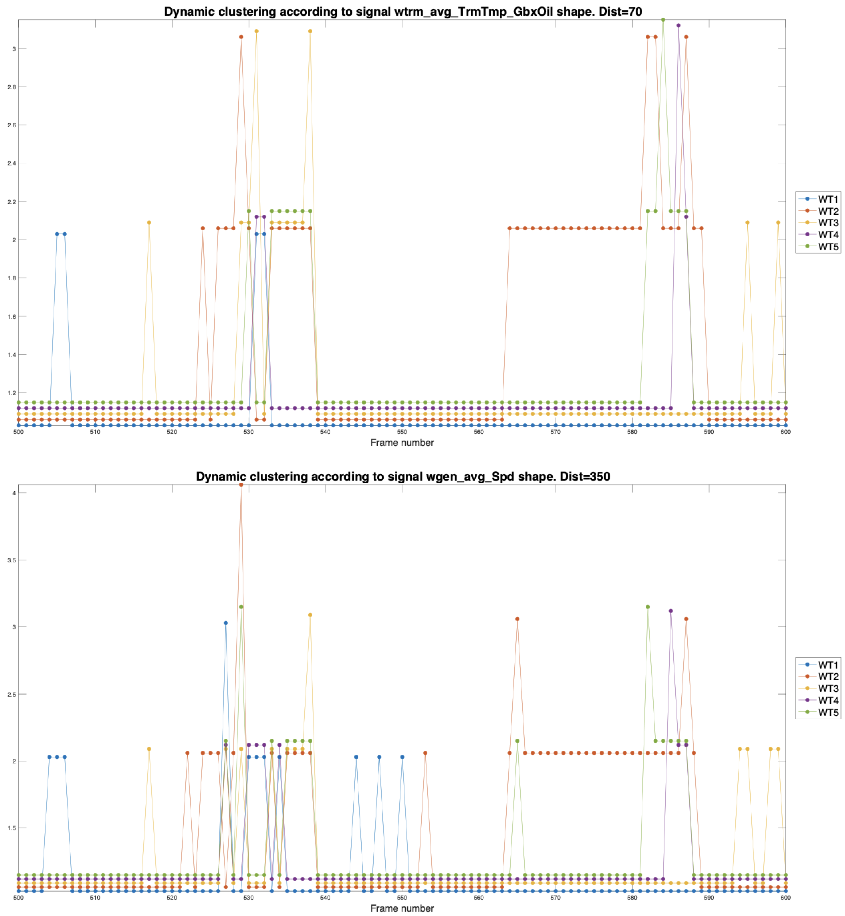
For example, WT2 and WT3 demonstrate a more apparent direct relationship when expanding the graphics between frames 500 and 600 in Figure 11, where one can observe the remarkable similarity of the signals in the oil and the rotational speed.
4. Conclusions
In this work, we propose a new methodology to cluster the WTs of a WF into clusters. It should be noted that the operation of wind turbines is highly non-linear and time-varying, so dynamic monitoring over time is required if we want to supervise them for a long time because conditions at different instants can be very different. The work is at an early stage, but the results we obtain show great potential. Below, we highlight the main contributions:
- (1)
- Clustering is based on a certain SCADA signal observed during a time interval, which we call a frame. It is done frame by frame, and it works for any averaged signal.
- (2)
- Compressing the information of the signals is critical, so the first coefficients of the DCT are used. With the DCT’s help, we represent each WT’s signals in low-dimensional vectors.
- (3)
- We use widely known agglomerative hierarchical clustering techniques and work with the Euclidean distance that we apply to the vectors of DCT coefficients. In a more advanced phase of knowledge, other distances can be explored. The advantage of these techniques is that they do not impose a fixed number of clusters. However, it is necessary to set a distance to prune the hierarchical trees. To explore the appropriate distance, we can use dendrogram-type representations. Once such distance is decided, it is maintained, and we use it to process all frames.
- (4)
- To keep an interpretable temporal track of the clusters frame by frame, it is crucial to define a stable cluster nomenclature. We use the information generated when the hierarchical tree is built from the distances between vectors according to a previously explained criterion. According to this nomenclature, the most similar signals are organized in low clusters and the most different in high clusters.
Due to the investigations’ initial state, different topics must be explored in more detail. For example, it should be noted that this approach may not fully capture complexities in waveforms depending on the signal analysed and their rapid transitions, thus implying more research on how best to select the appropriate number of DCT coefficients according to signal type, the length of the frame and operational conditions. Another point that may require a significant amount of research is the study of how to understandably represent dynamic WF diagrams with a more significant number of WTs and helpfully for making decisions, which indeed goes parallel to developing a form better to name the clusters.
In this work, however, one can already see the potential of the method presented by first analyzing an individual signal, such as the wind speed measured in the nacelles of the WTs, or the comparison of two critical variables, such as a rotation speed of the generator shaft or the gearbox oil temperature. Being able to know, for all critical variables, which are the WTs that deviate the most from normality, that is, from clusters 1 and 2, objectively can be an invaluable help to improve the preventive maintenance of the WFs.
Applying this clustering model in WF operational management could successfully plan preventive maintenance through early detection of abnormal conditions. Case studies have validated its practical applicability by reducing downtime and associated costs, demonstrating that this approach works. However, more research is needed on the scalability of the method and how it adapts to different WF configurations, especially concerning large and diverse farms. Limitations of the study are that large historical sets are required, and the input data must be very accurate. Still, the method proved to be strong for the WF investigated.
Funding
This research was supported by the Ministerio de Ciencia e Innovación of the Spanish Government (ref: PID2020-120314RB-I00).
Data Availability Statement
The data can be extracted from the freely available database at: https://github.com/alecuba16/fuhrlander
Acknowledgments
The author would like to thank the Smartive company (http://smartive.eu/) for providing the data used in the experimental part.
Conflicts of Interest
The authors declare no conflicts of interest
Abbreviations
The following abbreviations are used in this manuscript:
| DCT | Discrete cosine transform |
| HT | Hierarchical tree |
| HC | Hierarchical cluster |
| SCADA | Supervisory control and data acquisition |
| WF | Wind farm |
| WPC | Wind-power curve |
| WT | Wind turbine |
| WT81 | Wind turbine 81 |
| WT82 | Wind turbine 82 |
| WT83 | Wind turbine 83 |
| WT84 | Wind turbine 84 |
| WT85 | Wind turbine 85 |
References
- Surucu, O.; Gadsden, S.A.; Yawney, J. Condition monitoring using machine learning: A review of theory, applications, and recent advances. Expert Systems with Applications 2023, 221, 119738. [Google Scholar] [CrossRef]
- Pandit, R.; Astolfi, D.; Hong, J.; Infield, D.; Santos, M. SCADA data for wind turbine data-driven condition/performance monitoring: A review on state-of-art, challenges and future trends. Wind Engineering 2023, 47, 422–441. [Google Scholar] [CrossRef]
- Nunes, P.; Santos, J.; Rocha, E. Challenges in predictive maintenance–A review. CIRP Journal of Manufacturing Science and Technology 2023, 40, 53–67. [Google Scholar] [CrossRef]
- Zhou, Q.; Xiong, T.; Wang, M.; Xiang, C.; Xu, Q. Diagnosis and early warning of wind turbine faults based on cluster analysis theory and modified ANFIS. Energies 2017, 10, 898. [Google Scholar] [CrossRef]
- Du, B.; Narusue, Y.; Furusawa, Y.; Nishihara, N.; Indo, K.; Morikawa, H.; Iida, M. Clustering wind turbines for SCADA data-based fault detection. IEEE Transactions on Sustainable Energy 2022, 14, 442–452. [Google Scholar] [CrossRef]
- Ali, M.; Ilie, I.S.; Milanović, J.V.; Chicco, G. Probabilistic clustering of wind generators. In Proceedings of the IEEE PES General Meeting. IEEE; 2010; pp. 1–6. [Google Scholar]
- Blanco-M, A.; Gibert, K.; Marti-Puig, P.; Cusidó, J.; Solé-Casals, J. Identifying health status of wind turbines by using self organizing maps and interpretation-oriented post-processing tools. Energies 2018, 11, 723. [Google Scholar] [CrossRef]
- Rodriguez, P.C.; Marti-Puig, P.; Caiafa, C.F.; Serra-Serra, M.; Cusidó, J.; Solé-Casals, J. Exploratory analysis of SCADA data from wind turbines using the K-means clustering algorithm for predictive maintenance purposes. Machines 2023, 11, 270. [Google Scholar] [CrossRef]
- Liu, Y.; Gao, X.; Yan, J.; Han, S.; Infield, D.G. Clustering methods of wind turbines and its application in short-term wind power forecasts. Journal of Renewable and Sustainable Energy 2014, 6. [Google Scholar] [CrossRef]
- Teng, W.; Wang, X.; Meng, Y.; Shi, W. Dynamic clustering equivalent model of wind turbines based on spanning tree. Journal of Renewable and Sustainable Energy 2015, 7. [Google Scholar] [CrossRef]
- Wang, H.; Wang, H.; Jiang, G.; Li, J.; Wang, Y. Early fault detection of wind turbines based on operational condition clustering and optimized deep belief network modeling. Energies 2019, 12, 984. [Google Scholar] [CrossRef]
- Pei, M.; Ye, L.; Li, Y.; Luo, Y.; Song, X.; Yu, Y.; Zhao, Y. Short-term regional wind power forecasting based on spatial–temporal correlation and dynamic clustering model. Energy Reports 2022, 8, 10786–10802. [Google Scholar] [CrossRef]
- Paik, C.; Chung, Y.; Kim, Y.J. Power Curve Modeling of Wind Turbines through Clustering-Based Outlier Elimination. Applied System Innovation 2023, 6, 41. [Google Scholar] [CrossRef]
- Xie, W.B.; Lee, Y.L.; Wang, C.; Chen, D.B.; Zhou, T. Hierarchical clustering supported by reciprocal nearest neighbors. Information Sciences 2020, 527, 279–292. [Google Scholar] [CrossRef]
- Lee, H.G.; Piao, M.; Shin, Y.H. Wind power pattern forecasting based on projected clustering and classification methods. Etri Journal 2015, 37, 283–294. [Google Scholar] [CrossRef]
- Marti-Puig, P.; Blanco-M, A.; Cusidó, J.; Solé-Casals, J. Wind turbine database for intelligent operation and maintenance strategies. Scientific Data 2024, 11, 255. [Google Scholar] [CrossRef] [PubMed]
- Marti-Puig, P.; Hernández, J.Á.; Solé-Casals, J.; Serra-Serra, M. Enhancing Reliability in Wind Turbine Power Curve Estimation. Applied Sciences 2024, 14, 2479. [Google Scholar] [CrossRef]
- Kusiak, A.; Li, W. Short-term prediction of wind power with a clustering approach. Renewable Energy 2010, 35, 2362–2369. [Google Scholar] [CrossRef]
- Marti-Puig, P.; Bennásar-Sevillá, A.; Blanco-M, A.; Solé-Casals, J. Exploring the effect of temporal aggregation on SCADA data for wind turbine prognosis using a normality model. Applied Sciences 2021, 11, 6405. [Google Scholar] [CrossRef]
Figure 1.
Reconstruction of N=128 original signal points from L=2, 4 and 6 DCT coefficients.
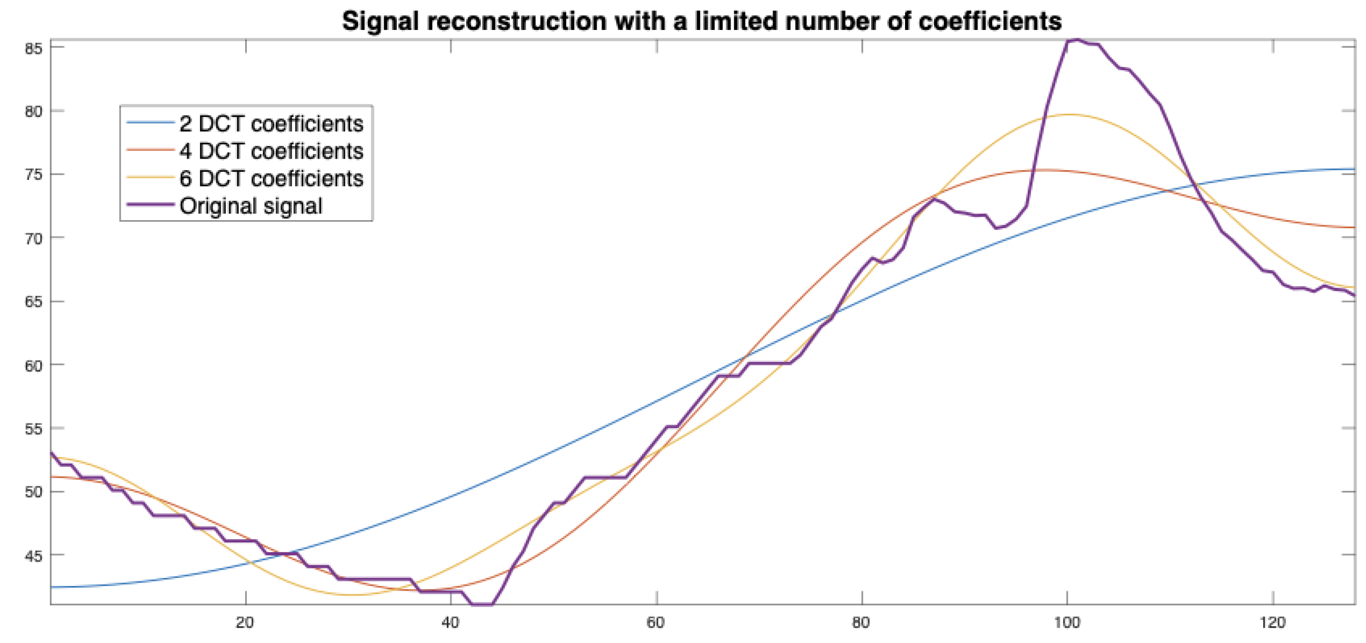
Figure 2.
This is a graphic representation of the main steps of the clustering of 5 temperature signals of 128 points using a vector of 3 DCT coefficients. Above are the original signs, and just below are reconstructions of the original signals based on just these three coefficients. On the bottom left is the HC represented as a dendrogram, and on the bottom right is the result of the clustering when using a threshold of 60.
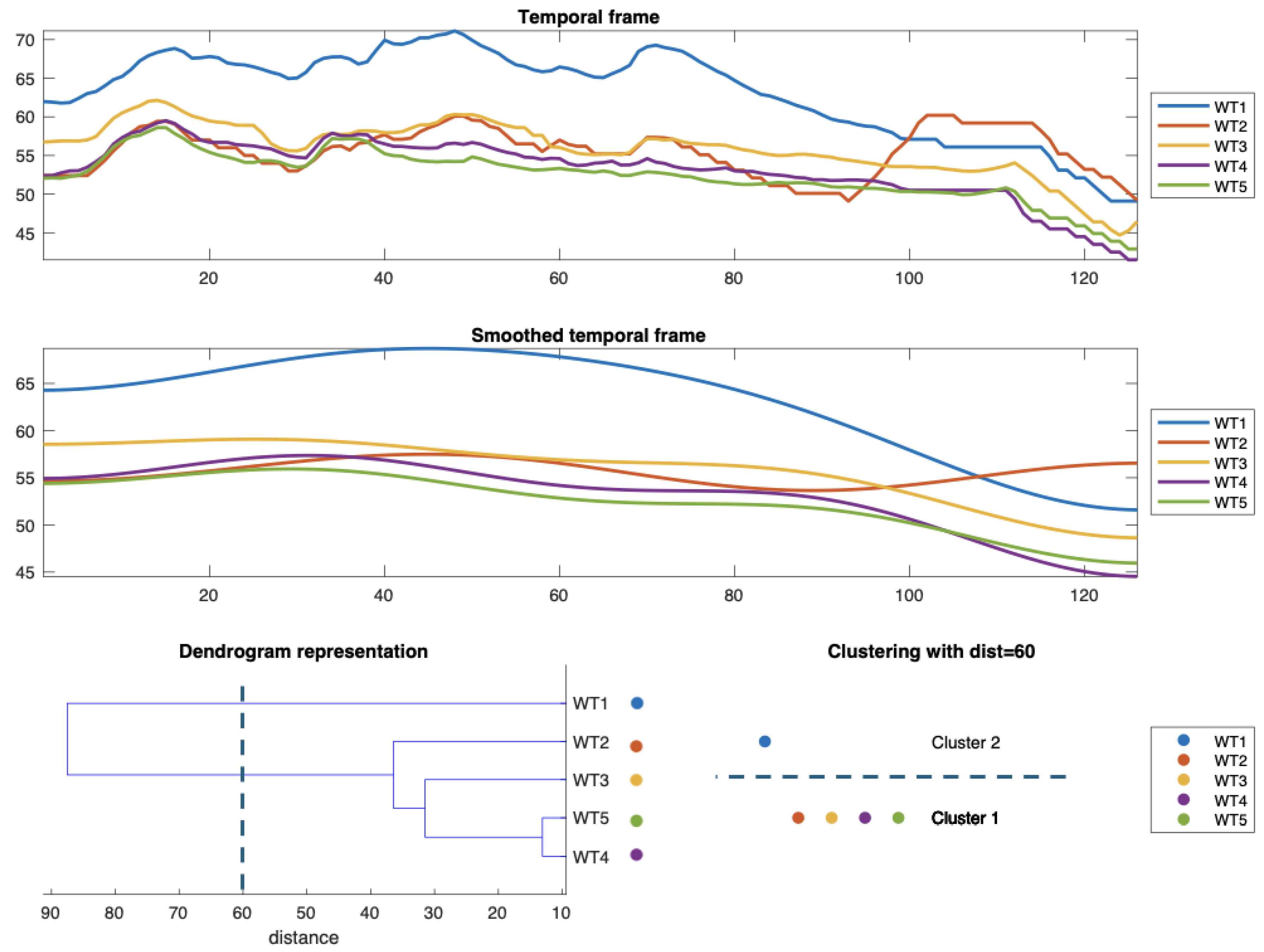
Figure 3.
Once the clusters have been formed, we sort them in the increasing order of the horizontal distances represented by the two-pointed arrows. The vertical line represents the distance used to prune the HT and form the clusters.
Figure 3.
Once the clusters have been formed, we sort them in the increasing order of the horizontal distances represented by the two-pointed arrows. The vertical line represents the distance used to prune the HT and form the clusters.
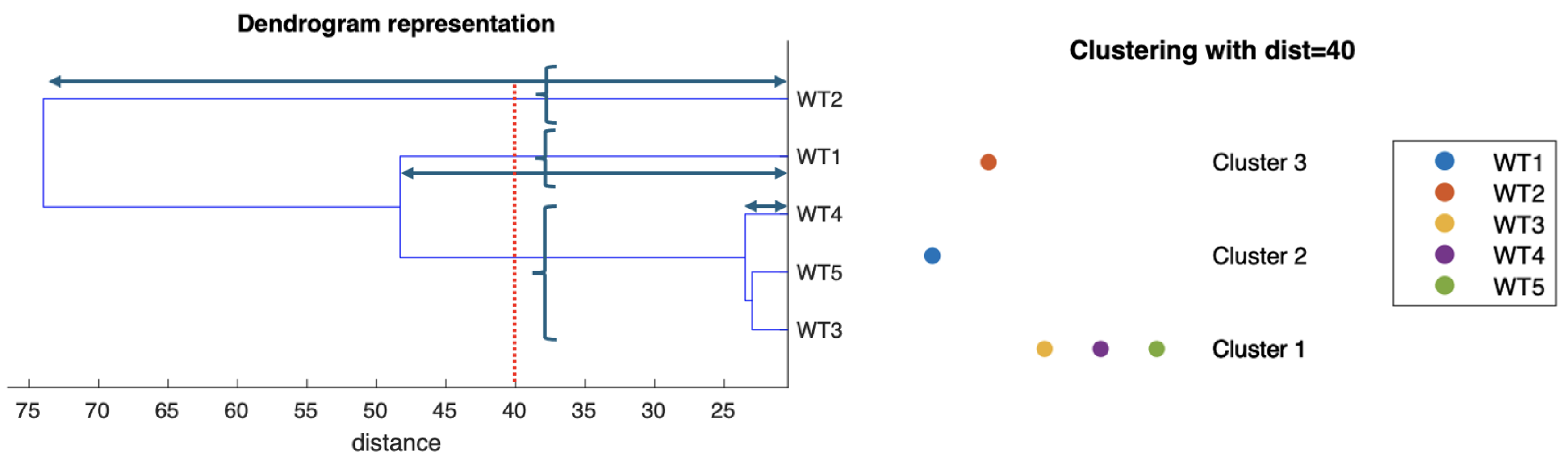
Figure 4.
a) Representation of the ordering of the clusters obtained by default after cutting the HTs. b) The arrangement we propose, based on the distances represented by black arrows on the dendrograms, aims to facilitate the interpretation of the evolution of the clusters over time. Notice that each WT is identified using a particular colour.
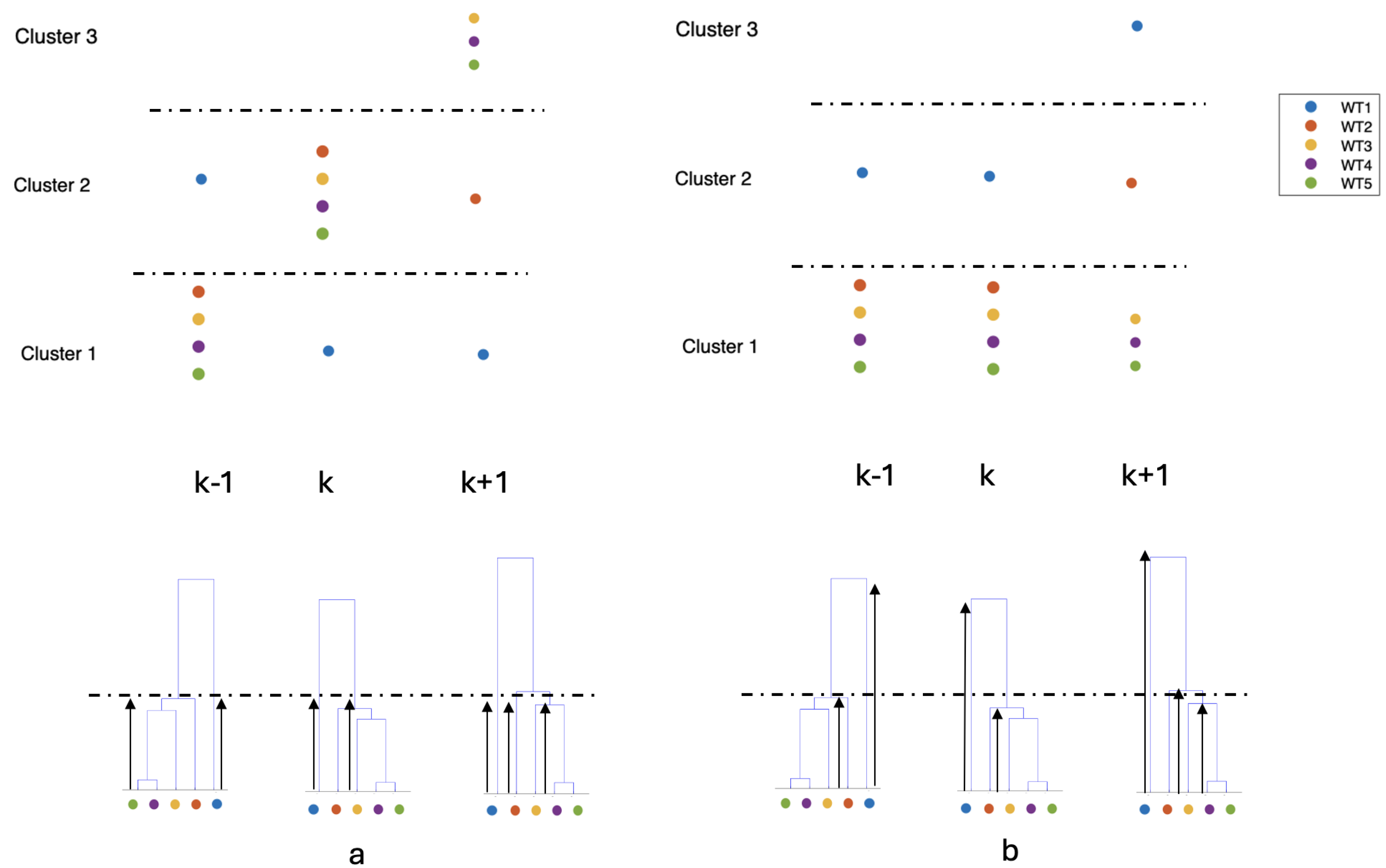
Figure 5.
Cluster’s dynamic evolution for the temperature signals . Each point represents a time window of 128 samples (640 minutes). The distance used to prune the HT is 120.
Figure 5.
Cluster’s dynamic evolution for the temperature signals . Each point represents a time window of 128 samples (640 minutes). The distance used to prune the HT is 120.
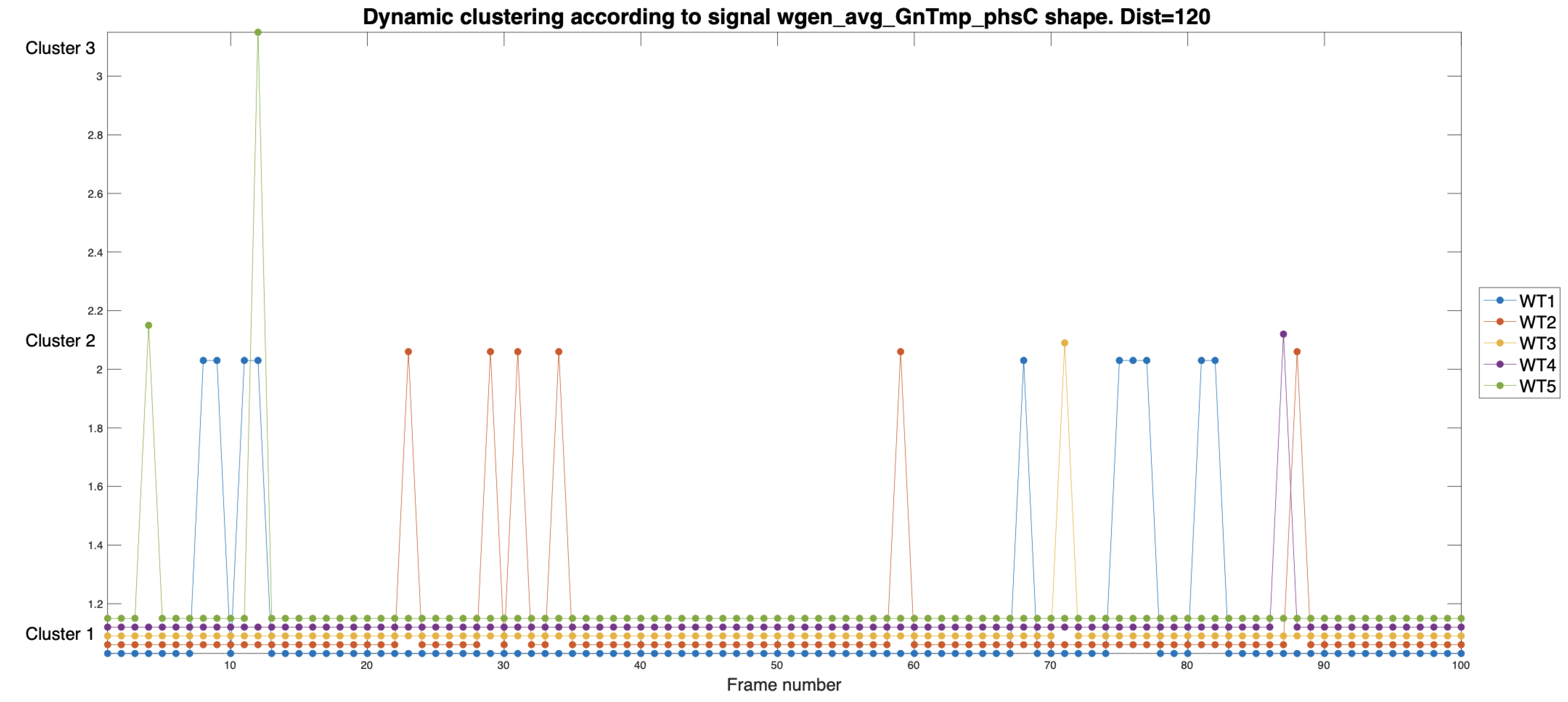
Figure 6.
Cluster’s dynamic evolution for the temperature signals . Each point represents a time window of 128 samples (640 minutes). The distance used to prune the HT is 40.
Figure 6.
Cluster’s dynamic evolution for the temperature signals . Each point represents a time window of 128 samples (640 minutes). The distance used to prune the HT is 40.
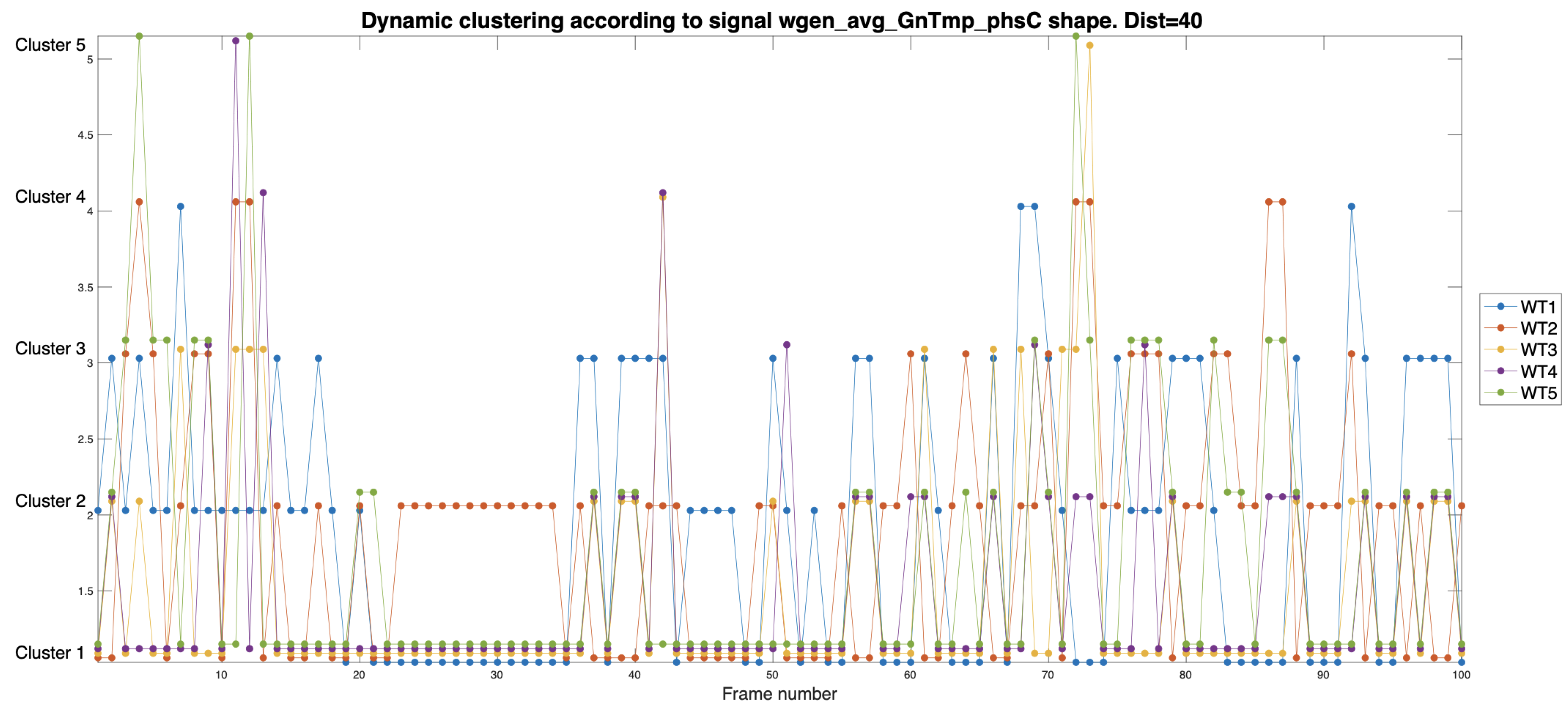
Figure 7.
Dynamic Clustering Analysis of the Wind Speeds measured in the nacelles by pruning the HT at distances of 20, 15 and 10, respectively.
Figure 7.
Dynamic Clustering Analysis of the Wind Speeds measured in the nacelles by pruning the HT at distances of 20, 15 and 10, respectively.
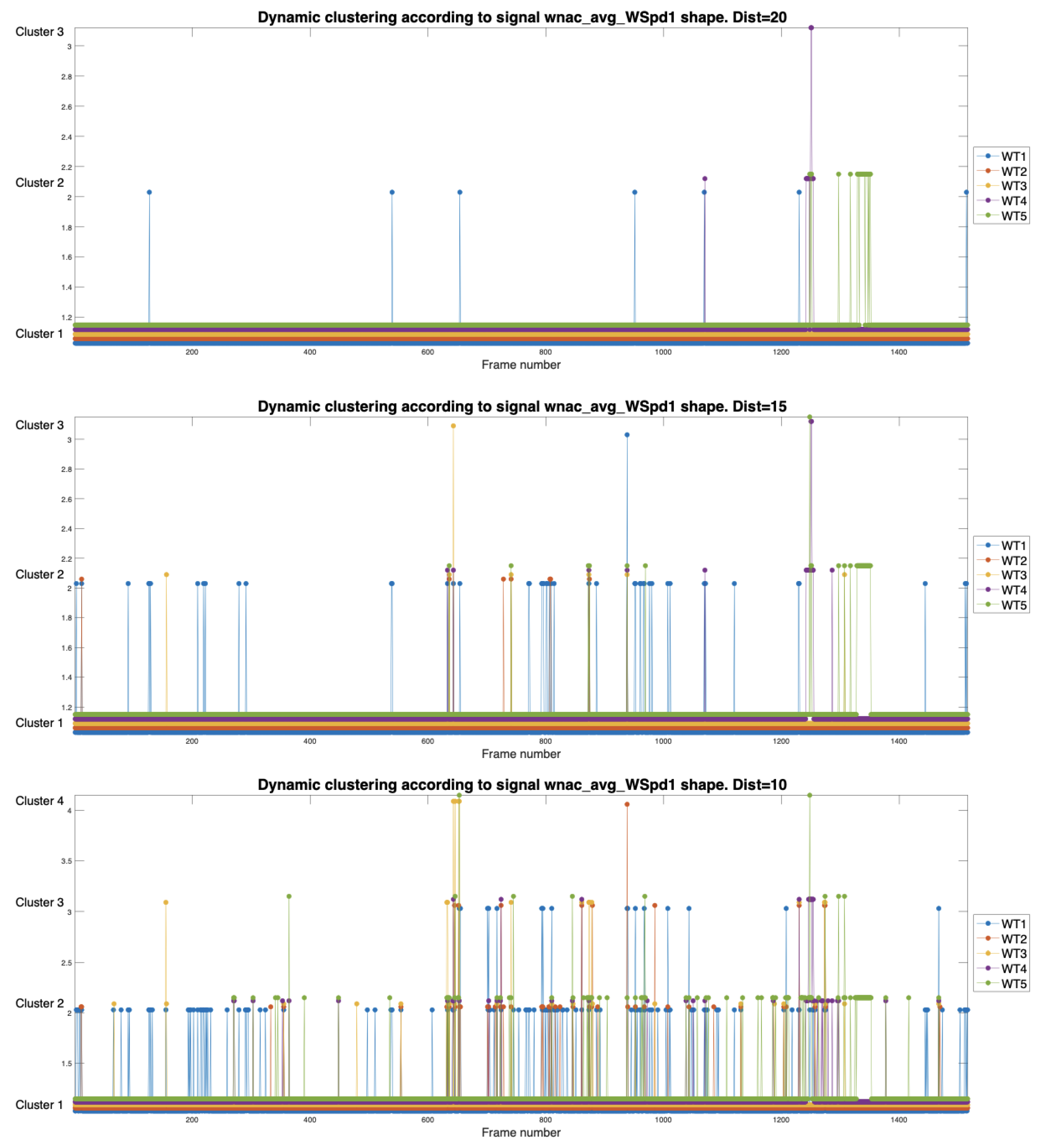
Figure 8.
Wind power curves of the WTs estimated from SCADA data. Graphic generated in [19].
Figure 8.
Wind power curves of the WTs estimated from SCADA data. Graphic generated in [19].
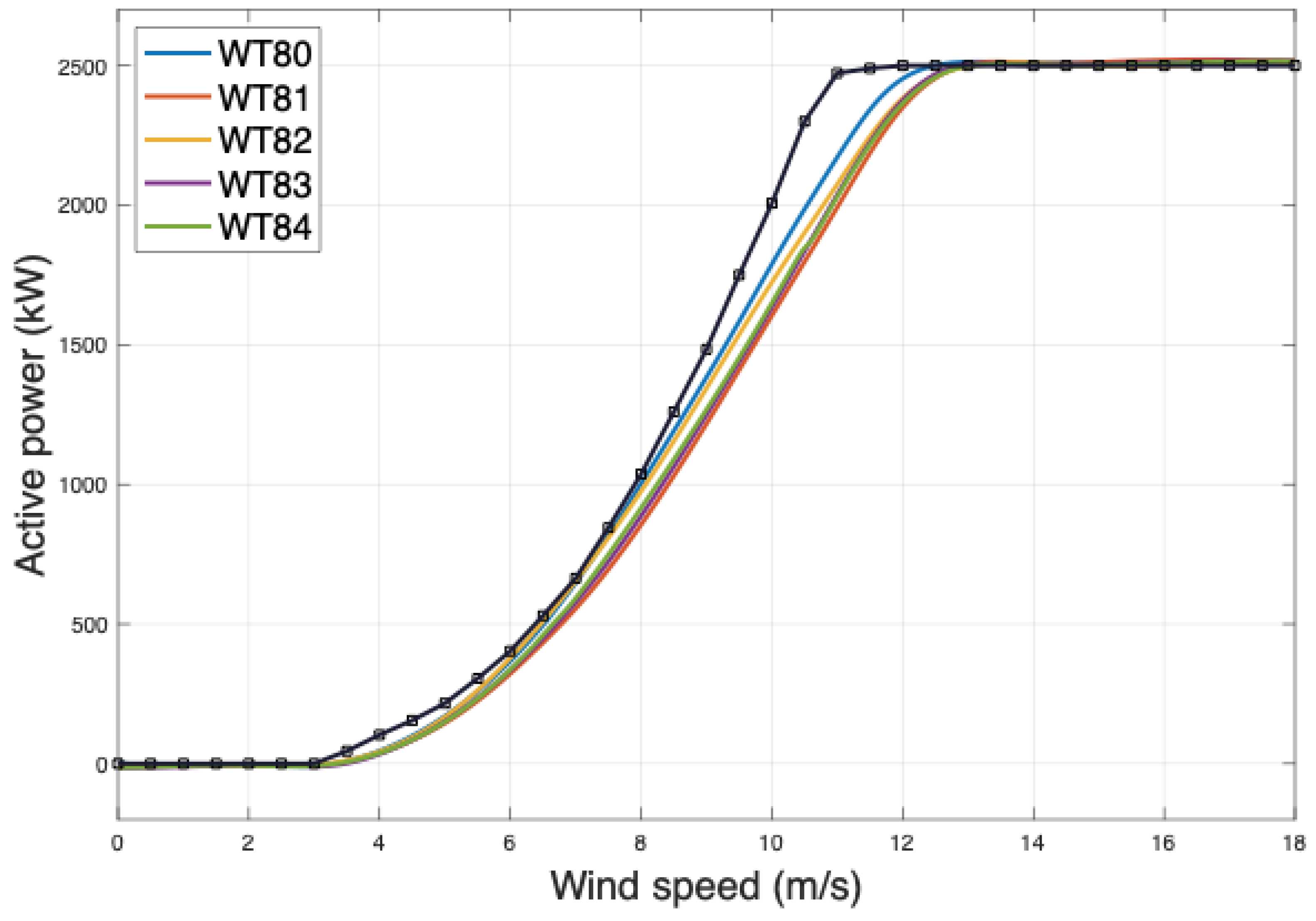
Figure 9.
Dynamic clustering of , the mean gearbox oil temperature performed by pruning the HTs with a distance of 120.
Figure 9.
Dynamic clustering of , the mean gearbox oil temperature performed by pruning the HTs with a distance of 120.
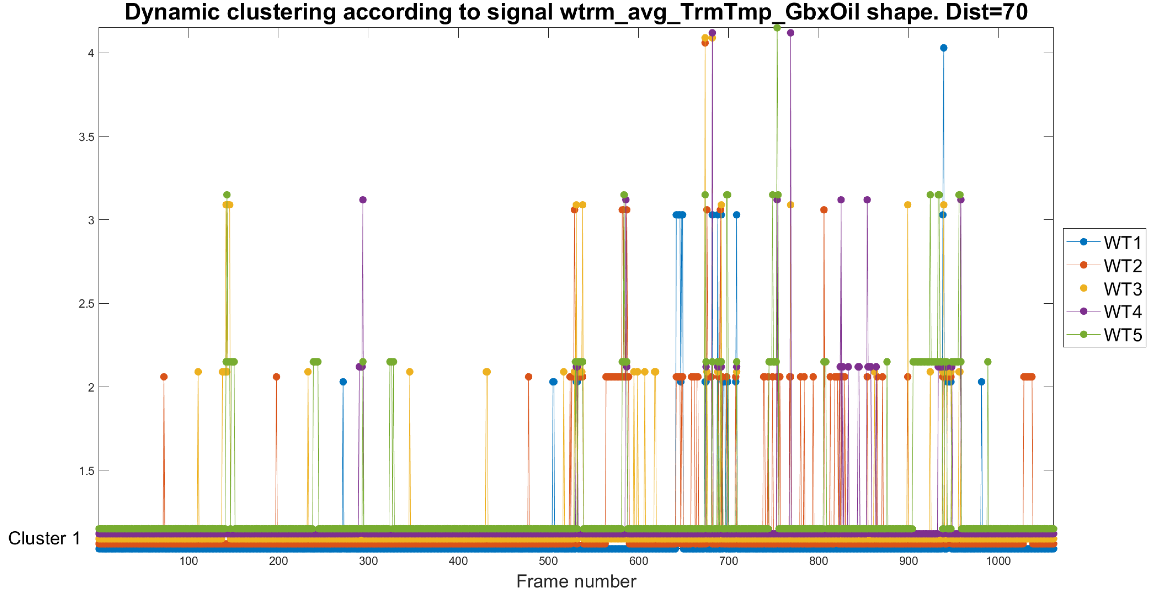
Figure 10.
Dynamic clustering of performed by pruning the HTs with a distance of 350.
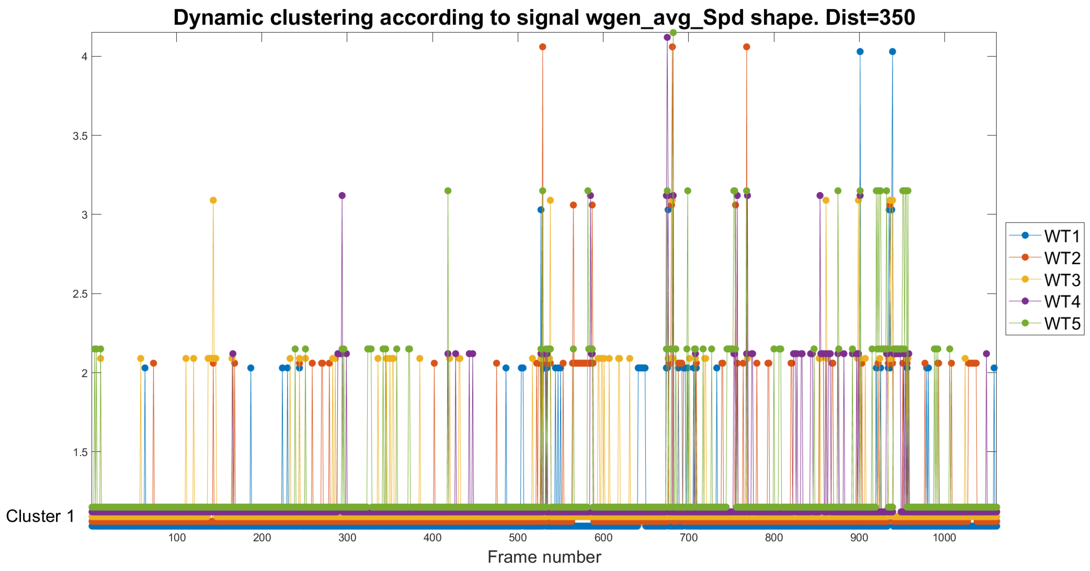
Figure 11.
Comparison of gearbox oil temperature and generator speed of the different WT’s studied. The analysis focuses on selected intervals for detailed inspection, revealing key patterns in operating behaviour that could influence equipment efficiency and maintenance.
Figure 11.
Comparison of gearbox oil temperature and generator speed of the different WT’s studied. The analysis focuses on selected intervals for detailed inspection, revealing key patterns in operating behaviour that could influence equipment efficiency and maintenance.
Disclaimer/Publisher’s Note: The statements, opinions and data contained in all publications are solely those of the individual author(s) and contributor(s) and not of MDPI and/or the editor(s). MDPI and/or the editor(s) disclaim responsibility for any injury to people or property resulting from any ideas, methods, instructions or products referred to in the content. |
© 2024 by the authors. Licensee MDPI, Basel, Switzerland. This article is an open access article distributed under the terms and conditions of the Creative Commons Attribution (CC BY) license (https://creativecommons.org/licenses/by/4.0/).
Copyright: This open access article is published under a Creative Commons CC BY 4.0 license, which permit the free download, distribution, and reuse, provided that the author and preprint are cited in any reuse.


