Submitted:
02 May 2024
Posted:
03 May 2024
You are already at the latest version
Abstract
Pinus occidentalis, Swartz is the primary timber species in the Dominican Republic (DR). Despite its economic importance, studies conducted on this species are very scarce, making it difficult to estimate current inventory levels. This study aims to enhance the accuracy of estimating total bole volume of P. occidentalis in different ecological zones (EZs) within La Sierra, evaluating and comparing two established volume equations—combined variable and Schumacher-Hall—across nine modeling variants (MVs). An indicator variables analysis determined the necessity of distinct equations for two EZs. Fitting included both linear and nonlinear models. Our comprehensive statistical analysis included goodness-of-fit metrics to evaluate each model variant's performance rigorously. Modeling variant SH02 was most effective in the Dry Ecological Zone, showing superior performance in both fitting and validation phases. Similarly, SH03 emerged as the best fit for the Combined Intermediate and Humid Ecological Zones, achieving the lowest overall ranking sum among tested variants. The SH equation variants SH02 and SH03, provide reliable and precise volume estimations, allowing optimization of forestry management practices for P. occidentalis trees. The SH models outperformed the CV model variants' consistency in parameter estimation. This tailored approach employed ensures more accurate volume predictions, which is crucial for sustainable management and conservation efforts.
Keywords:
indicator variables analysis
; ecological zones
; modeling variants
; goodness-of-fit
; volume estimation
; forestry management.
1. Introduction
Accurate measurements of tree dimensions like diameter, height, stem form, and volume are not just academic exercises, but crucial for estimating forest attributes. This research provides practical tools like individual-tree and species-specific volume equations, which are necessary to predict inventory levels and ensure long-term wood yields. Volume equations use DBH and height to calculate stem volume, providing reliable estimates of tree volumes by accounting for size and shape variations. These practical tools are essential in forestry practices, empowering forest managers and timber industry professionals with accurate and reliable data.
Stem volume models estimate timber volume, biomass, and carbon sequestration potential for individual trees and larger areas. They are useful in forest management planning and growth simulations, driven by the need for accurate estimation of tree bole volume. Because the same regression may not be equally suitable for predicting total volume estimates in different ecological conditions [1], specific details and techniques for developing statistical models for stem volume estimation may vary.
The history of excurrent tree bole volume estimation dates back several decades. Various statistical techniques can be used to develop stem volume models, including linear regression, nonlinear regression, mixed-effects procedures, and machine learning algorithms. The choice depends on the dataset’s underlying assumptions and characteristics [2]. They are developed in a two-step process: model fitting and validation. The model is fitted to the dataset using a statistical technique and then validated using an independent dataset. Evaluation uses measures such as mean squared error, root mean squared error, bias, and coefficient of determination.
The most common statistical procedure for developing volume tables is ordinary least squares (OLS) regression analyses, which relate bole volume to explanatory variables such as diameter-at-breast-height (DBH), height (H), and sometimes stem form. When dealing with biological data, the constant variance assumption is often violated whenever a direct measure of stem content is used as the dependent variable in a regression equation [3]. If the assumption of constant variance is unmet, the equation must be weighted by a factor proportional to the standard deviation of the dependent variable.
Weighted least squares can be used when the ordinary least squares assumption of constant variance in the errors is violated It will produce a new regression model which results in the dependent variable having constant variance [3]. In the weighted linear regression model, each observation is assigned a weight . The weighted sum of squared residuals, is minimized.
Assumptions related to linear and nonlinear statistical models involve linearity, independence, homoscedasticity, normality, and zero mean of residuals. Additionally, nonlinear models must have a correct expectation function [4]. These assumptions guide the development and application of these equations in forestry practices, and their violation may lead to biased predictions and incorrect inferences.
The scarcity of data on volume models for tropical and sub-tropical tree species negatively impacts the accuracy of estimating tree volume for both research and operational purposes [5]. Even when developed, stem volume models should be periodically updated to account for changes in forest structure, climate conditions, or management practices to ensure accurate predictions and relevant decision support. P. occidentalis is the main timber species in the DR, growing on approximately 302,500 hectares and comprising approximately 95% of all timber harvested [6]. Despite its economic importance, estimating inventory levels and accounting for harvested volume is difficult because no standardized system is used for volume appraisal and inventory purposes.
The Schumacher and Hall [7] equation (SH) has been widely used in forestry to estimate tree bole volumes. Other researchers have shown that this equation and the Combined Variable equation developed by Bennett et al. [8] provide accurate results for estimating tree volumes, good performance in graphical analysis, and reliable estimates without bias [9].
The objectives of this study were: (1) to fit two commonly used volume equations, the combined variable (CV) and the SH equations with nine different modeling alternatives (MV), to estimate total bole volume content of P. occidentalis trees growing in three ecological zones (EZ) within La Sierra, DR; (2) to evaluate goodness-of-fit statistics of these nine MVs in each EZ; (3) to conduct and indicator variable analysis to determine if separate equations were needed for each EZ; and (4); based on ranking of performance in terms of accuracy and precision, recommend the best MV alternative for estimating total bole volume in individual P. occidentalis trees.
2. Materials and Methods
The study area is located in the north-central part of Cordillera Central, DR, covering approximately 1,800 km2 (Figure 1). Even-aged natural stands of P. occidentalis are located within three ecological zones (EZs) according to the Holdridge [10] classification: Subtropical Dry Forest (DEZ), Subtropical Humid Forest (IEZ), and Subtropical Very Humid Forest (HEZ). Average elevations above sea level are 500, 650, and 800 m, respectively [11]. The climate varies depending on the altitude and precipitation. The average annual temperature is between 12ºC and 24ºC. These forests usually develop in shallow, carbonate, lateritic, low-producing soils with rugged topography.
2.1. Tree Data Sets
Three data sources were used for fitting total bole volume outside bark () models, one for each ecological zone (EZ). Trees from either dominant, intermediate, or overtopped classes in each zone were selected for destructive sampling, given that their phytosanitary status would allow it. After recording DBH outside bark at 1.30 m from the ground and measured with a diameter tape (0.1 cm precision), trees were felled as close to the ground as possible and H was measured with open-reel tape (0.1 cm precision). Besides DBH, other diameters were recorded at every meter along the bole from the base (10 cm above ground) up to the apex. Stem analysis data for model fitting purposes included 37 trees from the DEZ, 48 from the IEZ, and 72 from the HEZ. In addition, an independent data set collected from each zone was available to validate the resulting best total model. These data included 85, 90, and 75 independently measured P. occidentalis trees for the DEZ, IEZ, and HEZ. Table 1 showcases descriptive statistics for both the fitting and validation data set.
2.1. Data Exploration
To visualize the form of the relation between de dependent variable and the chosen explanatory variables DBH and total tree height (H), we proceeded to merge corresponding data from all three EZs and plot the against DBH first and later against D2H.
Approaches to Individual Tree Volume Prediction
2.1. Indicator Variables Analysis
An indicator variable analysis was conducted to check if three different equations were necessary for each EZ. We searched for statistically significant differences in the intercept and slope parameters in a regression equation fitted to the data for all three EZs, employing a single combined effect variable (D2H) and indicator variables. A statistically significant test for the intercept and/or the slope for two zones would indicate that each would require different equations. Equation [1] was used in the indicator variable analysis.
where,
- are as previously defined,
- are dichotomous variables,
- are parameters to be estimated,
2.1. Total Bole Volume Model Fitting
Observed outside bark bole volume (m3) computations were made using Smalian’s formula [12] for each 1 m section from the base to the apex, except for the last portion where the cone formula was used. The outside bark volume computed for each section was then summed up for each tree to calculate .
To estimate/predict of Pinus occidentalis individual trees, we choose two models,
The combined variable equation (CV):
- Schumacher and Hall’s (1933) equation (SH):
where
- total stem volume content outside bark (m3)
- normal diameter at 1.30 meters from the ground outside bark (cm)
- total tree height (m)
- natural logarithm
- error term.
- coefficients to be estimated.
We fitted five variants to our model [2] and four variants to our model [3], including linear, nonlinear, and weighted regression estimation techniques. The ordinary and weighted least squares method fitted the five Model [2] variants. These variants are:
- a.
- (CV01) Original equation
- b.
- Weighted linear regression using four different weights:
- (CV02) Weight 1 = 1/ Fitted Values from the original linear regression between the dependent variable “observed volume” (Vol), and the predictor normal diameter squared times total tree height (D2H).
- (CV03) Weight 2 = 1/fitted value resulting from fitting absolute values of original residuals against the fitted values of original combined variable regression.
- (CV04) Weight 3 = 1/fitted value resulting from fitting squared values of original residuals against the fitted values of original combined variable regression.
- (CV05) Weight 4 = 1/ , where the variance of ɛ is assumed to be proportional to [13].
Where
- CV0i = Variant identification code for model [2],
- C = exponent to be assumed or estimated.
The four variants from model [3] were fitted by the ordinary least squares and nonlinear methods, using multiple regression techniques between de dependent variable, , and the predictor variables, DBH and total tree height (H).
- (SH01) De-transformation of the logarithmic conversion (), solved by employing linear regression and correcting for bias. The correction is achieved by adding one-half of the estimated variance from the fitted regression before exponentiation [14]. The resulting expression is:
- = corrected estimate of the stem volume outside bark.
- = mean volume outside bark estimated in log scale.
- =half estimated variance in log scale.
2.1. Statistical Analysis
Weighted linear and nonlinear least squares were used to maximize the efficiency of parameter estimation. All tests on the full model parameters were conducted at α= 0.05. Data analysis and model development procedures were performed using lm, nls, and nlme commands in RStudio [15] to obtain parameter estimates for .
Starting values of the coefficients for nonlinear and weighted nonlinear variants were obtained by applying ordinary least squares to the log-transformed data, ensuring faster iteration. Even though log-transformed and nonlinear models are not mathematically equivalent, the coefficients of the former estimated by multiple regression may serve as starting values for the algorithm that estimates the coefficients of the latter [13].
To estimate coefficient c for the weighting of the observations in variants CV05 and SH04, observations were divided into five DBH classes containing approximately the same number of observations. Then, we calculated the standard deviation of in each D class. Following a methodology from Picard et al. [13], we plotted the standard deviation of against the median D in each of the five D in the log scale. The five points on the plot should be roughly aligned along a straight line to confirm that the power model was appropriate for modeling the residual variance. If that were the case, we would proceed to fit a linear regression of the log of the standard deviation of on the log of the median D for each class. The slope of such regression corresponds to exponent c. The standard deviation of the stem volume would be approximately proportional to D2C, and a weighting of the observations would be inversely proportional to it.
Statistical analyses performed on model [3] variant SH01 included initially working on the log-transformed data and fitting an ordinary least square (OLS) multiple regression of ln(V) against ln(D) and ln(H) and then transforming to original units the coefficient estimates of this initial equation and correcting it for bias by adding one-half of the estimated variance from the fitted regression before exponentiation.
2.1. Evaluation Criteria
2.1.1. Model Validation and Goodness of Fit Statistics
The goodness-of-fit statistics used to determine how well the regression functions fitted the sample data were (1) root mean square error (RMSE); (2) Bias; (3) the sum of squared relative residuals (SSRR); (4) the residual variance estimator (RVE), and (5) Akaike Information Criteria (AIC), used only in the fitting phase, to compare different models and balance goodness of fit with model complexity.
The “validation” statistics used to determine how well the regression functions performed on the independent data representing the population were (1) RMSE, (2) Bias, (3) SSRR, and (4) RVE. The best model for total bole volume in each of the three zones was selected based on the ranking of these evaluation criteria. We also considered the significance of parameter estimates [13,16]. Computational formulas for the goodness-of-fit statistics are:
where
: is the model’s likelihood,
p: is the number of free parameters estimated,
: is the observed stem wood volume outside bark,
: is the estimated stem wood volume outside bark,
: is the total number of observations,
: is the empirical variance of the response variable.
2.1.1. Ranking of Models
To rank the 9 MVs tested in each EZ, fit and validation goodness-of-fit statistics values were ranked. Rank valued 1 was linked to the best value for each of these statistics, rank No. 2 the second best, and so on. The overall rank for each model variant was determined by summing the ranks for the various goodness-of-fit statistics for total volume and then choosing the lowest sum as the best model variant.
2.1.1. Residual and QQ Plot Graphs
Scatterplots were constructed to check regression assumptions for the best-ranked MVs in the DEZ and CIHEZ zones to check that the hypotheses assumed for the residuals were satisfied.
The hypothesis that the residuals were independent has already been satisfied due to the sampling plan adopted. The constant variance hypothesis of the residuals was visually checked by plotting the cluster of points for the residuals in function to the predicted values. The hypothesis that the residuals are normally distributed was visually inspected with the quantile–quantile graphs, plotting the residuals’ empirical quantiles against the theoretical quantiles of the standard normal distribution. To further assess how well predictions from model variants align with the actual data, we plotted observed versus predicted stem volume values, and observed volumes versus predictor variables.
3. Results
3.1. Data Exploration
On average, sampled trees were smaller in terms of DBH, H, and in the DEZ, and largest in the HEZ. DBH ranged from 11.50 to 42.00 cm in the DEZ, from 16.50 to 53.50 cm in the IEZ, and from 21.50 to 46.50 cm in the HEZ. Following the same zone order, H from 10.30 to 24.00 m, 14.00 to 25.10 m, and 14.50 to 35.00 m. Volume outside bark ranged from 0.06 to 1.10 m3, 0.32 to 1.30 m3, and 0.20 to 2.73 m3, respectively (Table 1).
The cluster of points plotted to visualize the form of the relation between and DBH is depicted in the left side panel of Figure 2. It shows that the relation is not linear, and the volume variance increases with DBH. The relationship between against the combined effect variable D2H shown on the right side of Figure 2 shows that the relationship between these two variables is linear, but as before, the volume variance increases with D2H.
and DBH (left panel) and D2H. On the left, the relationship is nonlinear and presents heteroscedasticity. On the right, the relationship is linear, but heteroscedasticity persists.
3.1. Indicator Variables Analysis (IVA)
The results from IVA show that the HEZ and DEZ have different intercepts and the same slope. HEZ and IEZ have the same intercept and slope, and DEZ and IEZ zones have the same intercept but different slopes (Table 2). Therefore, the HEZ and IEZ can have the same equations to estimate of individual P. occidentalis trees, while the DEZ requires its own equations. Tree stem form has been observed to change in different zones with variation attributable to environmental factors [1]. Based on these IVA results, we combined the observed data from the HEZ and IEZ and fitted the tested models to the combined data.
Merged fitting data from the HEZ and IEZ totaled 121 observations. DBH ranged from 16.50 to 53.50 cm; H ranged from 14.00 to 35.00 m; and ranged from 0.20 to 2.76 m3. Respective averages and sample standard deviations (within parenthesis) were 31.77 cm, 22.67 m and 0.84 m3. After merging data from both zones, the validation data set had 165 observations with DBH ranging from 10.60 to 54.20 cm; H ranging from 9.40 to 27.80 m; and from 0.11 to 2.22 m3. Respective averages and sample standard deviations were 28.53 cm, 20.27 m, and 0.59 m3.
3.1. Total Bole Volume Model Fitting in the DEZ and the Combined IEZ and HEZ Ecological Zone (CIHEZ)
The SH02 variant fitted by non-linear least square (NLS) procedures, was ranked number one for estimating P. occidentalis in the DEZ; while in the CIHEZ, the best variant was SH03, which was fitted by weighted non-linear least squares (WNLS) procedures. Based on the ranks of goodness-of-fit statistics criteria applied to the data fitting and validation phases, these results indicate the superiority of the SH model variants in this study. The fitting and validation statistics values, along with rank sums and overall ranks for each MV in each EZ, are presented in Table 3 and Table 4.
Considering both the fitting and validation phases, SH02 in the DEZ was ranked No. 1 in terms of RMSE (0.0146) and RVE (0.0002) and No. 2 in AIC criteria (-199.86) in the fitting phase (Table 3). Likewise, it was ranked No. 1 in terms of RMSE (0.0702), Bias (-0.0099), and RVE (0.0030) in the validation phase. Percent bias calculated as in the fitting phase indicated that SH02 tends to overestimate slightly by approximately -0.059 %. Percent RMSE was calculated at 4.77% for SH02, suggesting that predictions deviate by about 4.77% from the mean of the actual values. We consider these values to be adequate for estimating for individual trees of P. occidentalis in this EZ.
SH02 had an overall sum rank of 31, being the lowest ranked of all volume variants tested in the DEZ. It was followed by SH04, the fourth variant of model (3) with a sum rank of 33 and fitted by WNLS procedure, where exponent “c” in the variance model (), was a parameter that needed to be estimated.
SH03 in the CIHEZ was ranked No. 1, achieving the lowest sum in the ranking (23) among the nine variants tested in this combined EZ (Table 4). For weights, the conditional standard deviation of derived from DBH is proportional to DBH4. In the fitting phase, SH03 was first regarding AIC criteria (-311.66). Similarly, it was ranked No. 1 in terms of RMSE (0.0943), Bias (-0.0614), and RVE (0.0059) in the validation phase. Percent bias calculated as in the fitting phase indicated that SH03 tends to underestimate on average by approximately 0.025%. Percentage RMSE was calculated at 8.96%, suggesting predictions that deviate by about 8.96% from the mean of the actual values for estimating for individual trees of P. occidentalis in the CIHEZ. Regarding the sum rank, SH03 was followed by MV SH01, the unweighted nonlinear version of the SHMV, with a sum rank of 35.
The parameterization of SH02 and SH03 are, respectively:
Although different fitting procedures estimated them, the intercept and coefficient corresponding to the DEZ and CIHEZ tree height are very similar. The intercepts differed by 2.54%, and the tree height (H) coefficients differed by 0.009%. The coefficients for D differed by 4.49%.
In checking regression assumptions, our plots show no curvature, although there is one point beyond the cutoff limit of two standard deviations in the top left panel corresponding to the DEZ. We assumed that MVs SH02 and SH03 do not seriously contradict the constant variance assumption. Even though the quantile–quantile plots of the residuals appear to have a slight structure in both zones, most of the points are aligned along a straight line and remain relatively consistent across all levels of the predictor variables, indicating that the constant variance assumption is sustained.
In Figure 3, scatter plots show randomly clustered values around the 1:1 line for outer bark volumes in the DEZ (top left) and the CIHEZ (bottom left). The points around the line remain relatively constant across all levels of the predictor variables, confirming the constant variance assumption and closely following the observed values, suggesting that these models capture the variability in the data well.
In Figure 4, the top right panel shows predictions made by MV SH02 against predictors DBH and H in the DEZ. Likewise, the bottom right panel shows the predictions made by MV SH03 against the same predictors in the CIHEZ. These plots to the right support observations in the left panel graphs by showing the agreement between predictions and measured variables. SH02 and SH03 efficiently estimated stem volume outside bark for P. occidentalis in both EZs and effectively captured the variability in the data.
4. Discussion
Alvarado-Segura et al. [17] used a nonlinear version of the SH model to estimate the stem volume of Pinus patula Schiede ex Schlechtendal et Chamisso var. Patula, in Hidalgo, Mexico and reported an RMSE of 0.0914. Our RMSE statistic value is much better for our SH02 MV (0.0146), while the corresponding value for SH03 (0.0943) is close to that reported by these authors. The SH model has been found to perform well in predicting stem volume for many species and genera in diverse environments [18]. Castillo-López et al. [19] and Valerio-Hernández et al. [19] used this model in studying volume equations for pine species in Mexico and Nicaragua. Based on the evaluation criteria, this study’s nonlinear version (SH02) and the nonlinear weighted variant (SH03) of the SH model performed best.
All nine variants tested from models (2) and (3) in both EZs resulted in parameter estimates that are statistically significant and logically consistent for outside bark volume estimation (Table 5 and Table 6). The estimates for intercept, interpreted as the average value of total stem volume accumulated by a tree until it reaches breast height (when DBH is zero and total height is 1.3 m) were positive and significantly different from zero. All other parameters were consistent in terms of sign and magnitude.
The best-ranked Combined Variable model variant was CV02 which achieved an overall ranking of 3 in the DEZ and 4 in the CIHEZ. Values for intercept coefficients of variants in model (2) resemble in a certain way the shape and form of a geometric solid, with higher numbers representing better and more cylindrical form and thus greater volume [12]. On average, model (2) variants intercepts are lower (105.77%) in the DEZ than their counterparts in the CIHEZ, indicating that stem volume accumulated by individual P. occidentalis trees below breast height is lower in the former zone. A t-test assuming unequal variances indicates that intercepts from the two zones are statistically and significantly different (P=0.0026). Slope coefficients for D2H in the same model (2) variants are also statistically and significantly different (P=0.000126).
In mathematics, the volume of a circular base solid with base diameter D and height H is expressed as: [21]. If the diameter is measured in cm, for a cylinder, for a paraboloid, for a cone, and for a neiloid. This is equivalent to , the coefficient in the second term of the CV. The averages of the five values from our results are equivalent to 0.0000347 in the DEZ, and 0.0000321 in the CIHEZ, differing by about 12.4 % and 20.47% off the perfect paraboloid, respectively. Similar values for using the CV equation in fitting data from 150 P. patula trees were found by Alvarado-Segura et al. [17] in Mexico. Therefore, tree shapes in our study approximate a paraboloid solid, which is described mathematically by the expression π/80000 = 0.0000393 (diameters are in cm units). This contrasts with the results of Sharma [21] who found that the shape of the trees is not a solid described by a cylinder, paraboloid, cone, or neiloid while assessing tree volume of several species in natural stands of Canada and northeastern United States.
Differences in the parameters of the CV models between EZs may result from differences in the height-dbh relationship, tree form, tree taper, or a combination of these factors [1], although all were logically consistent. These results agree with the findings reported by Sharma [22], who employed the CV equation to compare goodness-of-fit statistics, logical consistency, and predictive accuracy of several models in Pinus resinosa Sol. ex Aiton. Exploratory analyses of variance not reported in the study showed that the form and quotient coefficients of P. occidentalis trees in these zones were statistically significant. That, combined with higher values for the coefficient in the HEZ Zone may indicate that the form may be better there.
5. Conclusions
Nine model variants (MVs), five from the CV and four from the SH, were evaluated in their capacity to estimate stem volume outside bark (SVOB) of individual P. occidentalis trees growing in natural stands within three EZs in La Sierra, D.R. All variants produced results consistent with those of other pine species. All MVs gave good results on the fitting dataset, but the performance was poorer when used in the validation dataset. Ercanli et al. [23] and Sahin [24] encounter the same situation while modeling tree volume of conifer species in Turkey.
An indicator variable analysis indicated that only one equation was required to estimate SVOB in the IEZ and HEZ. Therefore, observations from these two EZs were combined to evaluate the different MVs further.
The CV model variants were logically consistent in parameter estimation. They complied with regression assumptions but were inferior to the chosen SHVE model variants regarding a ranking based on goodness-of-fit statistics and predictive ability. MVs SH02 and SH03, strategies for modeling individual P. occidentalis trees were efficient and selected as the volume equations for the DEZ and CIHEZ, respectively.
The maximum bias among all MVs in the DEZ was 0.20% and 5.54% in the fitting and validation phases, respectively. Likewise, in the CIHEZ, bias was 0.007% and 8.84%, respectively. According to Sharma [21], volume equations resulting in a bias larger than 10% should not be recommended for forest management decision-making. The minimum observed variability explained by all variants in both zones was 94% for outside bark volume estimates.
Developing forest management strategies requires accurate tree volume estimates, employing tools such as tree volume models. These volume models are simpler to use if the entire stem volume is of interest [25]. As the assumptions underlying the regression methods employed in the study for constructing these nine volume model variants were validated, and the results showed that these MVs performed well in both the fitting and validation phases, we propose their use as useful tools for predicting total stem volume outside bark in these EZs within La Sierra, D.R. The equations presented here provide a more scientifically accurate and consistent predictions of individual P. occidentalis trees. They are a valuable tool for supporting present and future management decisions.
Author Contributions
Conceptualization, S.W.B.L. and J.G.T.H.; methodology, S.W.B.L. and L.R.C.R.; validation, S.W.B.L. and L.R.C.R..; formal analysis, S.W.B.L..; investigation, S.W.B.L..; data curation, S.W.B.L. and J.G.T.H..; writing—original draft preparation, S.W.B.L., L.R.C.R. and J.G.T.H.; writing—review and editing, S.W.B.L.; project administration, S.W.B.L.; funding acquisition, S.W.B.L. and L.R.C.R. All authors have read and agreed to the published version of the manuscript.
Funding
This research was funded by the Ministry of Higher Education, Science and Technology of the Dominican Republic, grant number FONDOCyT 2018. The APC was funded by Pontificia Universidad Católica Madre y Maestra (PUCMM).
Data Availability Statement
The authors will make the raw data supporting this article’s conclusions available upon request.
Acknowledgments
We recognize the effort and contribution of the acquisitions department of PUCMM and the administrative staff of the Vice-Rectory of Research and Innovation at PUCMM. We are also grateful to José Reyes and Roque Herrera, who assisted us in field data collection.
Conflicts of Interest
The authors declare no conflicts of interest.
References
- Kangas, A.; Pitkänen, T.P.; Mehtätalo, L.; Heikkinen, J. (2023) Mixed linear and non-linear tree volume models with regional parameters to main tree species in Finland, Forestry: An International Journal of Forest Research, 96:2, 188–206, https://doi.org/10.1093/forestry/cpac038. [CrossRef]
- Li, R.; Weiskittel, A.R. (2010) Comparison of model forms for estimating stem taper and volume in the primary conifer species of the North American Acadian Region. Ann. For. Sci. 67:302. https://doi.org/10.1051/forest/2009109. [CrossRef]
- Clutter, J.L.l; Fortson, J.C.; Pienaar, L.V.; Brister, G.H.; Bailey, R.L. (1983) Timber management: a quantitative approach. (First edition) Krieger Publishing Company, Malabar, Florida. 333 p.
- Bates, D.M.; Watts, D.G. (2014) Nonlinear Regression Analysis and its Applications (First ed.). Wiley India Pvt. Ltd., John Wiley & Sons, Inc., New York. 365 p.
- Vibrans, A.C.; Moser, P.; Oliveira, L.Z.; Maçaneiro, J.P. (2016) Generic and specific stem volume models for three subtropical forest types in southern Brazil. Annals of Forest Science. https://doi.org/10.1007/s13595-015-0481-x. [CrossRef]
- MMARN - MINISTERIO DE MEDIO AMBIENTE Y RECURSOS NATURALES (2021). Inventario Nacional Forestal de la República Dominicana. Programa Regional de Reducción de Emisiones de la Deforestación y Degradación de Bosques en Centroamérica y Republica Dominicana (REDD III). Santo Domingo, República Dominicana. 292 pp.
- Schumacher, F.X.; Hall, F.S. (1933) Logarithmic expression of timber-tree volume. Journal of Agricultural Research. 47:9, 719–734.
- Bennett, F.A.; McGee, C.E.; Clutter, J.L. (1959) Yield of old-field slash pine plantations. U.S.D.A. For. Serv., S. E. For. Exp. Stn. Paper No. 107.
- Azevedo, G.B.; Tomiazzi, H.V.; Azevedo, S.; Pereira, L.; Teodoro, R.; Pereira de Souza, T.; Silva, T.; Philipe, B.; Guerra, S. (2020) Multi-volume modeling of Eucalyptus trees using regression and artificial neural networks PLOSONE. 1- 17. https://doi.org/10.1371/journal.pone.0238703. [CrossRef]
- Holdridge, L. (1987) Ecología basada en zonas de vida. First edition. Instituto Interamericano de Cooperación para la Agricultura, San José, Costa Rica. 304 p.Abreu JC, Soares CPB, Leite HG, Binoti DHB and Silva GF (2020) Alternatives to estimate the volume of individual trees in forest formations in the state of Minas Gerais-Brazil. CERNE, 26:3, 393-402. https://doi.org/10.1590/01047760202026032728. [CrossRef]
- Bueno-López, S.W. (2009) Understanding Growth and Yield of Pinus Occidentalis, Sw. in La Sierra, Dominican Republic (Doctor of Philosophy Degree Dissertation). State University of New York College of Environmental Science and Forestry. Syracuse. New York. 256 p.
- Burkhart, H.E.; Tomé, M. (2012). Modeling Forest Trees and Stands. First edition. Springer Science & Business Media. 457 p. https://doi.org/10.1007/978-90-481-3170-9. [CrossRef]
- Picard, N.; Saint-André, L.; Henry, M. (2012) Manual for building tree volume and biomass allometric equations: from field measurement to prediction. (First edition) Food and Agricultural Organization of the United Nations, Rome, and Centre de Coopération Internationale en Recherche Agronomique pour le Développement, Montpellier. 215 pp.
- Flewelling, J.W.; Pienaar, L.V. (1981) Multiplicative regression with lognormal errors. Forest Science 27:3, 281-289.
- RStudio Team (2020) RStudio: Integrated Development for R. RStudio, PBC, Boston, MA URL http://www.rstudio.com/.
- Hu, N. (2003) Development of a new variable-form taper equation to investigate differences in stem form following release in eastern white pine (Pinus strobus L.). (Master of Science Thesis). State University of New York; College of Environmental Science and Forestry, Syracuse, New York. 97p.
- Alvarado-Segura, A.A.; Zamudio-Sánchez, F.J.; De La Cruz-De La Cruz, K,I, (2020) A Procedure For Choosing Tree-Stem Volume Equations Previously Fitted in a Forest. Journal of Sustainable Forestry. 1 – 14. https://doi.org/10.1080/10549811.2020.1711776. [CrossRef]
- Abreu, J.C.; Soares, C.P.B.; Leite, H.G.; Binoti, D.H.B.; Silva, G.F. (2020) Alternatives to estimate the volume of individual trees in forest formations in the state of Minas Gerais-Brazil. CERNE. 26:3, 393-402. https://doi.org/10.1590/01047760202026032728. [CrossRef]
- Castillo-López, A.; Quiñonez-Barraza, G.; Diéguez-Aranda, U.; Corral-Rivas, J.J. (2021) Compatible Taper and Volume Systems Based on Volume Ratio Models for Four Pine Species in Oaxaca Mexico. Forests 12, 145. https://doi.org/10.3390/f12020145. [CrossRef]
- Valerio-Hernández, L.A.; Campos-Vanegas, W.A.; Cruz-Tórrez, L.E.; Pena-Ortiz, J.A.; Vargas-Larreta, B. (2024) Improving Volume and Biomass Equations for Pinus oocarpa in Nicaragua. Forests, 15, 309. https://doi.org/10.3390/f15020309. [CrossRef]
- Sharma, M. (2021) Total and Merchantable Volume Equations for 25 Commercial Tree Species Grown in Canada and the Northeastern United States. Forests, 12, 1270. https://doi.org/10.3390/f12091270. [CrossRef]
- Sharma, M. (2020) Increasing Volumetric Prediction Accuracy: An Essential Prerequisite for End-Product Forecasting in Red Pine. Forests, 11,1050; https://doi.org/10.3390/f11101050. [CrossRef]
- Ercanli, I.; Senyurt, M.; Bolat, F. (2022). A major challenge to machine learning models: compatible predictions with biological realism in forestry: a case study of individual tree volume. In: Proceeding of the “3rd International Conference on Environment and Forest Conservation (ICEFC)”. Kastamonu (Turkey) 21-23 Feb 2022, pp. 39.
- Sahin, A. (2024). Analyzing regression models and multi-layer artificial neural network models for estimating taper and tree volume in Crimean pine forests. iForest 17: 36-44. – doi: 10.3832/ifor4449-017. [CrossRef]
- Sharma, M. (2019) Inside and outside bark volume models for jack pine (Pinus banksiana) and black spruce ( Picea mariana ) plantations in Ontario, Canada. The Forestry Chronicle 95:01, 50-57. https://doi.org/10.5558/tfc2019-009. [CrossRef]
Figure 1.
Study area within La Sierra region in the north-central portion of Cordillera Central, Dominican Republic.
Figure 1.
Study area within La Sierra region in the north-central portion of Cordillera Central, Dominican Republic.
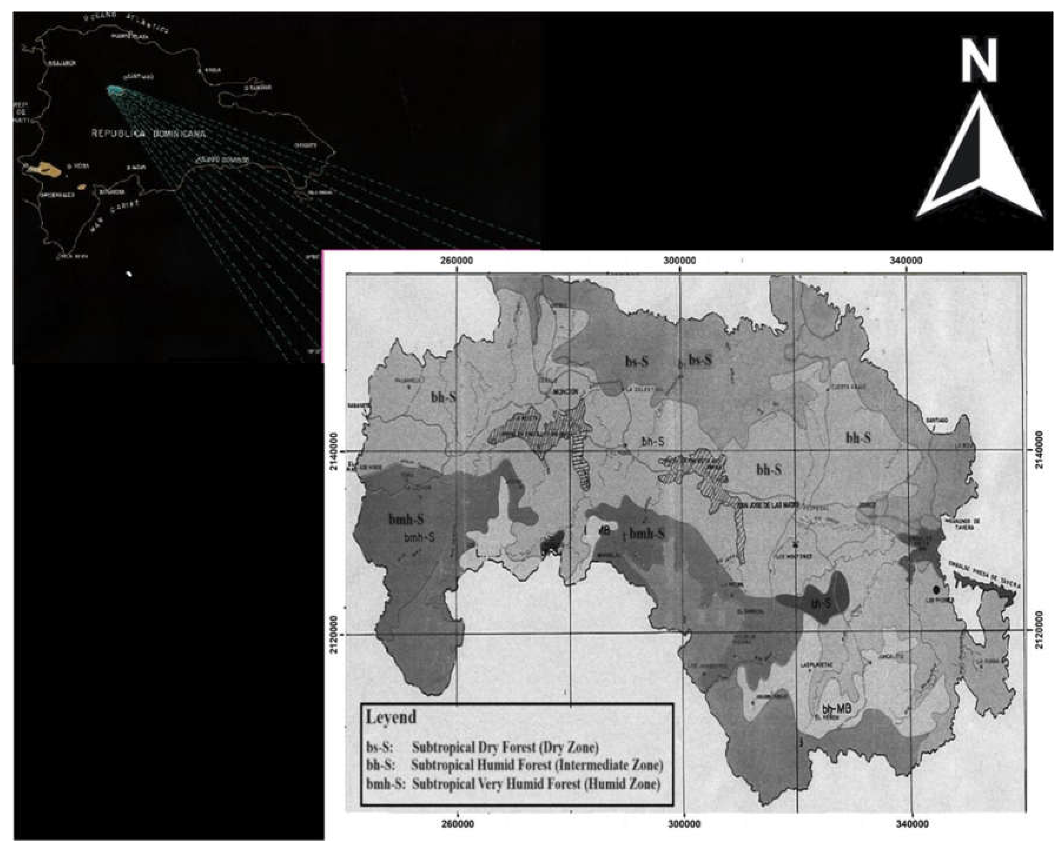
Figure 2.
Scatterplots of the relation between
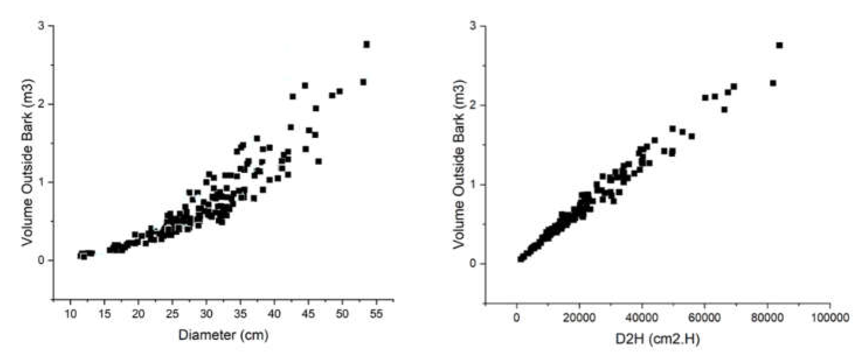
Figure 3.
Standardized residuals plotted against fitted values and quantile–quantile plots as tools to check constant variance and normal distribution hypotheses of the residuals in the DEZ and CIHEZ using MVs SH02 and SH03. Residuals versus fitted values in the DEZ (top) and CIHEZ (bottom) are shown on the left. Sample versus theoretical quantiles in the DEZ (top) and CIHEZ (bottom) are depicted on the right.
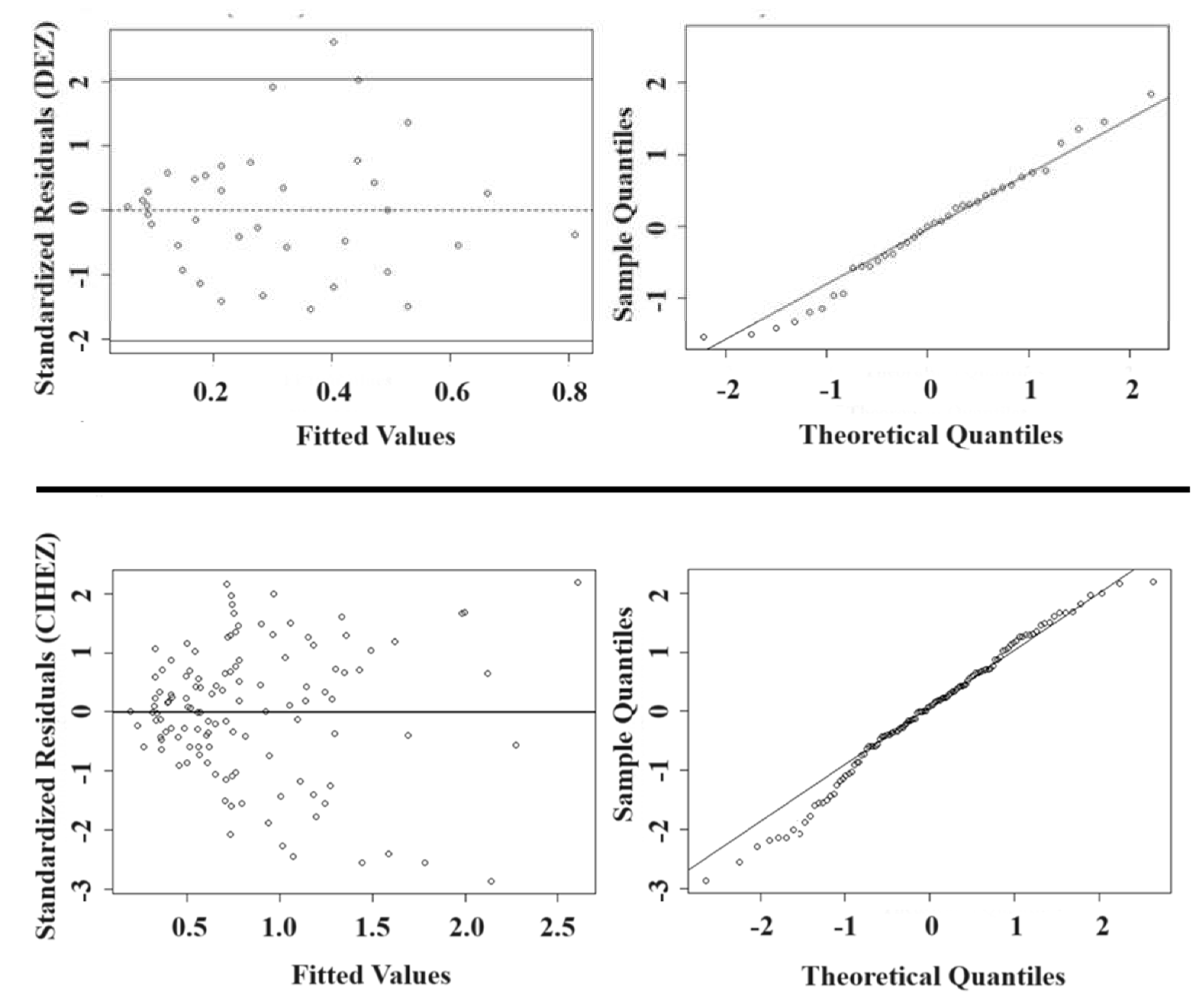
Figure 4.
Predicted outside bark volumes plotted against corresponding observed volumes (left), and predicted volumes plotted versus predictor variables DBH and H, for P. occidentalis in the DEZ. The solid 45-degree line in the left panel represents the 1:1 line for outside bark volumes. On the left, observed volume (m3) versus predicted volumes in the DEZ (top) and CIHEZ (bottom) are illustrated. Observed volume versus predictor variables in the DEZ (top) and CIHEZ (bottom) are shown on the right.
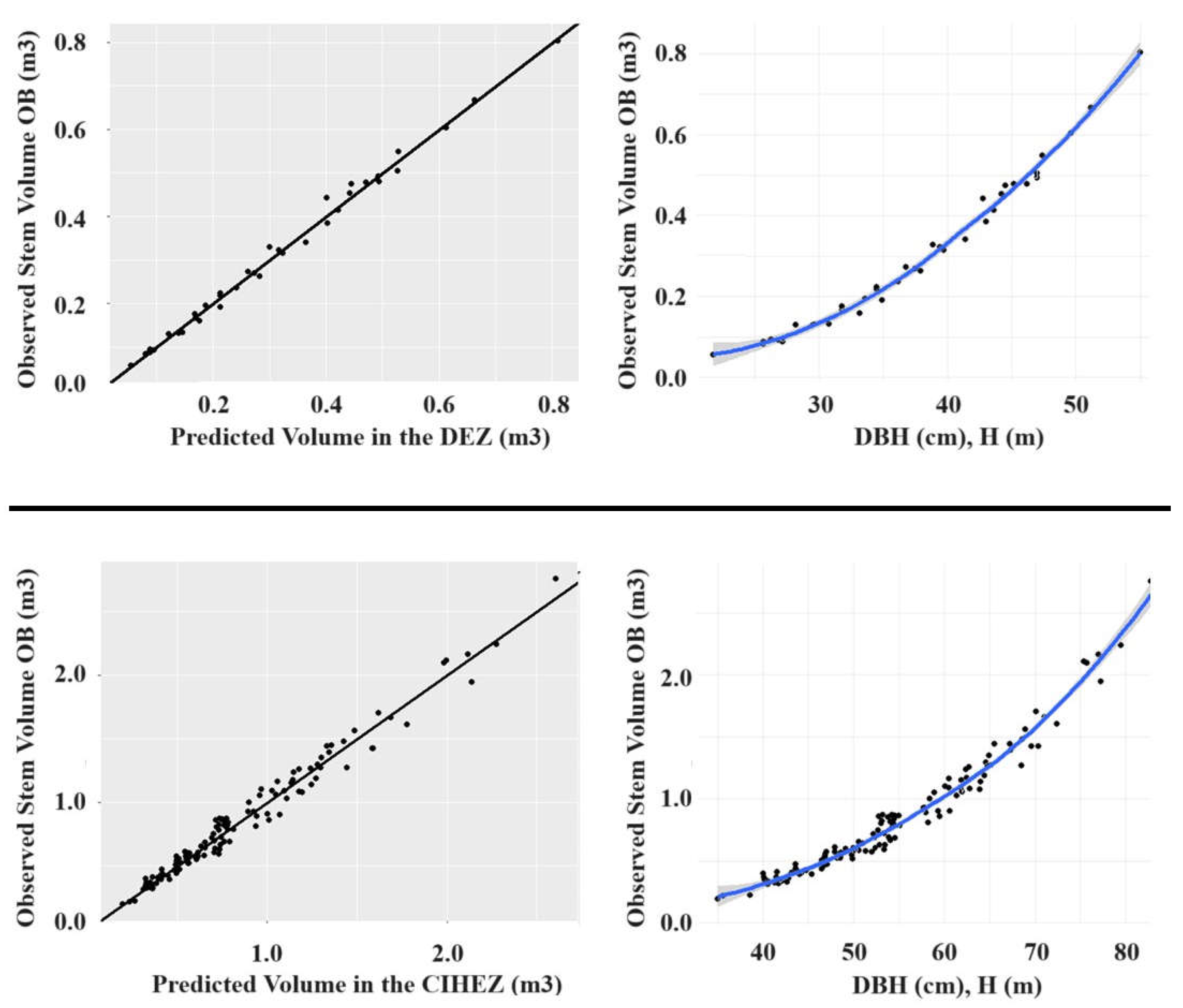

Table 1.
Descriptive statistics of tree measurements in each ecological zone for the fitting and validation data sets used in the study.
Table 1.
Descriptive statistics of tree measurements in each ecological zone for the fitting and validation data sets used in the study.
| Variable | Ecological Zone | n | Mean | Std Dev | Minimum | Maximum |
|---|---|---|---|---|---|---|
| Fitting Data Set | ||||||
| Diameter (cm) | DEZ | 37 | 22.13 | 6.57 | 11.50 | 42.00 |
| IEZ | 48 | 32.63 | 8.34 | 16.50 | 53.50 | |
| HEZ | 72 | 31.18 | 5.18 | 21.50 | 46.50 | |
| Height (m) | DEZ | 37 | 16.49 | 2.92 | 10.30 | 24.00 |
| IEZ | 48 | 19.78 | 2.78 | 14.00 | 25.10 | |
| HEZ | 72 | 24.65 | 4.76 | 14.50 | 35.00 | |
| Volume (m3) | DEZ | 37 | 0.34 | 0.22 | 0.06 | 1.10 |
| IEZ | 48 | 0.66 | 0.24 | 0.32 | 1.30 | |
| HEZ | 72 | 0.98 | 0.57 | 0.20 | 2.76 | |
| Validation Data Set | ||||||
| Diameter (cm) | DEZ | 85 | 21.32 | 7.95 | 8.00 | 42.10 |
| IEZ | 90 | 27.26 | 8.20 | 11.00 | 54.20 | |
| HEZ | 75 | 30.06 | 7.87 | 10.60 | 50.10 | |
| Height (m) | DEZ | 85 | 16.33 | 4.46 | 7.30 | 26.10 |
| IEZ | 90 | 19.96 | 4.06 | 10.10 | 27.80 | |
| HEZ | 75 | 20.65 | 3.40 | 9.40 | 27.40 | |
| Volume (m3) | DEZ | 85 | 0.35 | 0.25 | 0.10 | 1.23 |
| IEZ | 90 | 0.55 | 0.35 | 0.12 | 2.22 | |
| HEZ | 75 | 0.64 | 0.36 | 0.11 | 1.81 | |
Table 2.
Statistical test results for the intercept and slope coefficients from the Indicator Variable Analysis of the dependent variable Stem Volume Outside Bark in the three ecological zones.
Table 2.
Statistical test results for the intercept and slope coefficients from the Indicator Variable Analysis of the dependent variable Stem Volume Outside Bark in the three ecological zones.
| Zone Analysis | Intercept | Slope |
|---|---|---|
| HEZ versus DEZ | Different: = 0.0277 | Same: =0.1414 |
| HEZ versus IEZ | Same: = 0.4851 | Same: =0.974 |
| DEZ versus IEZ | Same: = 0.104 | Different: =0.0294 |
Table 3.
Goodness-of-fit statistics and ranking were obtained in the fitting and validation stage of five variants of the Combined Variable Equation and four of the Schumacher and Hall model to estimate stem volume outside bark of P. occidentalis trees in the DEZ within La Sierra, Dominican Republic.
| Fit Statistics | Validation Statistics | Ranking | ||||||||||
|---|---|---|---|---|---|---|---|---|---|---|---|---|
| Model | Variant Code | RMSE (Rank) | BIAS (Rank) | SSRR (Rank) | RVE (Rank) | AIC (Rank) | RMSE (Rank) | BIAS (Rank) | SSRR (Rank) | RVE (Rank) | Sum Rank | Overall Rank |
| Model (2): Effect Variable D2H | CV01 | 1.61E-02 | 3.87E-19 | 1.06E-01 | 2.82E-04 | -1.95E+02 | 7.92E-02 | -1.32E-02 | 5.98E+00 | 3.52E-03 | 46 | 6 |
| (5) | (1) | (9) | (9) | (8) | (4) ) |
(5) | (1) | (4) | ||||
| CV02 | 1.62E-02 | 9.96E-19 | 9.66E-02 | 2.80E-04 | -2.07E+02 | 8.11E-02 | -1.28E-02 | 6.41E+00 | 3.63E-03 | 38 | 3 | |
| (6) | (2) | (6) | (5) | (4) | (5) ) |
(3) | (2) | (5) | ||||
| CV03 | 1.62E-02 | -2.41E-04 | 9.67E-02 | 2.80E-04 | -2.06E+02 | 8.21E-02 | -1.37E-02 | 6.42E+00 | 3.71E-03 | 53 | 7 | |
| (7) | (6) | (7) | (6) | (5) | (7) | (6) | (3) | (6) | ||||
| CV04 | 1.63E-02 | -5.93E-04 | 9.57E-02 | 2.81E-04 | -2.12E+02 | 8.31E-02 | -1.38E-02 | 6.59E+00 | 3.77E-03 | 58 | 8 | |
| (9) | (8) | (4) | (8) | (1) | (8) | (7) | (5) | (8) | ||||
| CV05 | 1.63E-02 | -6.83E-04 | 9.62E-02 | 2.81E-04 | -2.11E+02 | 8.32E-02 | -1.42E-02 | 6.51E+00 | 3.77E-03 | 61 | 9 | |
| (8) | (9) | (5) | (7) | (2) | (9) | (8) | (4) | (9) | ||||
| Model (3): Effect Variables D, H | SH01 | 1.48E-02 | 2.70E-04 | 9.55E-02 | 2.49E-04 | -1.08E+02 | 7.36E-02 | -1.30E-02 | 7.20E+00 | 3.19E-03 | 41 | 4 |
| (4) | (7) | (1) | (4) | (9) | (3) | (4) | (6) | (3) | ||||
| SH02 | 1.46E-02 | -1.81E-04 | 9.85E-02 | 2.39E-04 | -2.00E+02 | 7.02E-02 | -9.89E-03 | 7.28E+00 | 2.97E-03 | 31 | 1 | |
| (1) | (5) | (8) | (1) | (6) | (1) | (1) | (7) | (1) | ||||
| SH03 | 1.47E-02 | -6.23E-06 | 9.56E-02 | 2.43E-04 | -2.11E+02 | 8.14E-02 | -1.89E-02 | 7.33E+00 | 3.71E-03 | 44 | 5 | |
| (3) | (3) | (2) | (3) | (3) | (6) | (9) | (8) | (7) | ||||
| SH04 | 1.47E-02 | -2.54E-05 | 9.56E-02 | 2.42E-04 | -1.97E+02 | 7.15E-02 | -1.02E-02 | 7.33E+00 | 3.06E-03 | 33 | 2 | |
| (2) | (4) | (3) | (2) | (7) | (2) | (2) | (9) | (2) | ||||
CV01: Combined Variable (OLS); CV02: Combined Variable (W1); CV03: Combined Variable (W2); CV04: Combined Variable (W3); CV05: Combined Variable (W2); SH01: De-transformed S & H Model with Bias Corrected; SH02: S & H Non-linear Model; SH03: S & H Weighted Non-linear Model Assuming Exponent C; SH04: S & H Weighted Non-linear Model Modeling Exponent C; OLS: Ordinary Least Squares; WLS: OLS*: Ordinary Least Squares (Retransformed and Corrected for Bias); Weighted Least Squares; NLS: Nonlinear Least Squares; WNLS: Weighted Nonlinear Least Squares; ML: Maximum Likelihood Estimation; DBH: Normal Diameter at 1.30 m aboveground; H: Total Tree Height.
Table 4.
Goodness-of-fit statistics and respective ranking obtained in the fitting and validation stage of five variants of the Combined Variable Equation and four variants of the Schumacher and Hall model to estimate stem volume outside bark of P. occidentalis trees in the CIHEZ within La Sierra, Dominican Republic.
| Fit Statistics | Validation Statistics | Ranking | |||||||||||
|---|---|---|---|---|---|---|---|---|---|---|---|---|---|
| Model | Variant Code | RMSE (Rank) | BIAS (Rank) | SSRR (Rank) | RVE (Rank) | AIC (Rank) | RMSE (Rank) | BIAS (Rank) | SSRR (Rank) | RVE (Rank) | Sum Rank | Overall Rank | |
| Model (2): Effect Variable D2H | CV01 | 7.85E-02 | 6.11E-18 | 1.06E+00 | 6.31E-03 | -2.67E+02 | 1.01E-01 | -7.29E-02 | 2.22E+00 | 6.70E-03 | 50 | 7 | |
| (5) | (2) | (9) | (9) | (8) | (4) | (8) | (1) | (4) | |||||
| CV02 | 7.87E-02 | -4.01E-18 | 1.01E+00 | 6.19E-03 | -2.99E+02 | 1.03E-01 | -7.06E-02 | 2.39E+00 | 6.84E-03 | 41 | 4 | ||
| (6) | (1) | (7) | (6) | (5) | (5) | (4) | (2) | (5) | |||||
| CV03 | 7.89E-02 | -1.29E-03 | 1.01E+00 | 6.17E-03 | -3.01E+02 | 1.06E-01 | -7.24E-02 | 2.56E+00 | 7.17E-03 | 49 | 6 | ||
| (7) | (7) | (6) | (5) | (3) | (6) | (5) | (3) | (7) | |||||
| CV04 | 8.08E-02 | -5.31E-03 | 1.00E+00 | 6.19E-03 | -3.11E+02 | 1.14E-01 | -7.27E-02 | 3.23E+00 | 7.81E-03 | 59 | 8 | ||
| (9) | (8) | (5) | (7) | (2) | (9) | (6) | (5) | (8) | |||||
| CV05 | 8.07E-02 | -7.43E-03 | 1.02E+00 | 6.21E-03 | -3.00E+02 | 1.14E-01 | -7.43E-02 | 3.10E+00 | 7.85E-03 | 67 | 9 | ||
| (8) | (9) | (8) | (8) | (4) | (8) | (9) | (4) | (9) | |||||
| Model (3): Effect Variables D, H | SH01 | 7.59E-02 | -5.22E-04 | 9.56E-01 | 5.94E-03 | -2.39E+02 | 9.49E-02 | -6.17E-02 | 4.14E+00 | 6.02E-03 | 35 | 2 | |
| (4) | (5) | (1) | (4) | (9) | (2) | (2) | (6) | (2) | |||||
| SH02 | 7.55E-02 | 6.86E-04 | 9.57E-01 | 5.86E-03 | -2.74E+02 | 9.86E-02 | -6.53E-02 | 4.33E+00 | 6.41E-03 | 36 | 3 | ||
| (1) | (6) | (2) | (3) | (7) | (3) | (3) | (8) | (3) | |||||
| SH03 | 7.56E-02 | 2.08E-04 | 9.65E-01 | 5.83E-03 | -3.12E+02 | 9.43E-02 | -6.14E-02 | 4.22E+00 | 5.97E-03 | 23 | 1 | ||
| (2) | (4) | (4) | (2) | (1) | (1) | (1) | (7) | (1) | |||||
| SH04 | 7.56E-02 | -9.23E-05 | 9.65E-01 | 5.81E-03 | -2.98E+02 | 1.08E-01 | -7.27E-02 | 4.75E+00 | 7.43E-03 | 45 | 5 | ||
| (3) | (3) | (3) | (1) | (6) | (7) | (7) | (9) | (6) | |||||
CV01: Combined Variable (OLS); CV02: Combined Variable (W1); CV03: Combined Variable (W2); CV04: Combined Variable (W3); CV05: Combined Variable (W2); SH01: De-transformed S & H Model with Bias Corrected; SH02: S & H Non-linear Model; SH03: S & H Weighted Non-linear Model Assuming Exponent C; SH04: S & H Weighted Non-linear Model Modeling Exponent C; OLS: Ordinary Least Squares; WLS: OLS*: Ordinary Least Squares (Retransformed and Corrected for Bias); Weighted Least Squares; NLS: Nonlinear Least Squares; WNLS: Weighted Nonlinear Least Squares; ML: Maximum Likelihood Estimation; DBH: Normal Diameter at 1.30 m aboveground; H: Total Tree Height.
Table 5.
Parameter estimates, corresponding confidence intervals, residual standard error, and adjusted coefficient of determination obtained in fitting five variants of the Combined Variable Equation and four variants of the Schumacher and Hall model to estimate stem volume outside bark of P. occidentalis trees in the DEZ, La Sierra, Dominican Republic.
| CV (Model (2)) | S & H (Model (3)) | |||||||||
|---|---|---|---|---|---|---|---|---|---|---|
| Parameters | Statistics | CV01 | CV02 | CV03 | CV04 | CV05 | SH01 | SH02 | SH03 | SH04 |
| Residual Est. Error | 1.66E-02 | 2.79E-02 | 1.25E+00 | 6.07E+01 | 6.87E-05 | 1.48E-02 | 1.52E-02 | 3.16E-05 | 1.47E-02 | |
| Adjusted R2 | 9.92E-01 | 9.93E-01 | 9.92E-01 | 9.92E-01 | 7.60E-01 | 9.93E-01 | 9.93E-01 | 9.93E-01 | 9.93E-01 | |
| B0 | Estimate | 1.59E-02 | 1.35E-02 | 1.34E-02 | 1.25E-02 | 1.29E-02 | 6.14E-05 | 5.81E-05 | 5.88E-05 | 5.84E-05 |
| Lower Bound 95% CI | 5.54E-03 | 6.80E-03 | 6.36E-03 | 7.69E-03 | 7.66E-03 | 4.69E-05 | 4.29E-05 | 4.48E-05 | 5.84E-05 | |
| Upper Bound 95% CI | 2.63E-02 | 2.02E-02 | 2.05E-02 | 1.73E-02 | 1.81E-02 | 8.04E-05 | 7.85E-05 | 7.71E-05 | 5.84E-05 | |
| Pr(>|t|) Bo | 3.66E-03 | 2.43E-04 | 4.72E-04 | 6.80E-06 | 1.49E-05 | 5.59E-39 | 1.02E-07 | 1.00E-08 | 9.99E-09 | |
| B1 | Estimate | 3.44E-05 | 3.46E-05 | 3.47E-05 | 3.48E-05 | 3.48E-05 | 1.82E+00 | 1.78E+00 | 1.82E+00 | 1.81E+00 |
| Lower Bound 95% CI | 3.33E-05 | 3.37E-05 | 3.36E-05 | 3.38E-05 | 3.38E-05 | 1.73E+00 | 1.67E+00 | 1.72E+00 | 1.81E+00 | |
| Upper Bound 95% CI | 3.54E-05 | 3.56E-05 | 3.57E-05 | 3.59E-05 | 3.58E-05 | 3.63E+00 | 1.89E+00 | 1.91E+00 | 1.81E+00 | |
| Pr(>|t|) B1 | 1.44E-38 | 1.51E-39 | 1.11E-38 | 7.22E-39 | 5.88E-40 | 1.52E-30 | 1.07E-27 | 2.04E-30 | 2.97E-30 | |
| B2 | Estimate | 1.02E+00 | 1.08E+00 | 1.04E+00 | 1.04E+00 | |||||
| Lower Bound 95% CI | 8.79E-01 | 9.64E-01 | 8.95E-01 | 1.04E+00 | ||||||
| Upper Bound 95% CI | 2.04E+00 | 1.19E+00 | 1.18E+00 | 1.04E+00 | ||||||
| Pr(>|t|) B2 | 3.88E-16 | 9.02E-20 | 1.75E-16 | 1.35E-16 | ||||||
| C | Estimate | 1.74E+00 | 2.00E+00 | 1.90E+00 | ||||||
Table 6.
Parameter estimates, corresponding confidence intervals, residual standard error, and adjusted coefficient of determination obtained in fitting five variants of the Combined Variable Equation and four variants of the Schumacher and Hall model to estimate stem volume outside bark of P. occidentalis trees in the CIHEZ, La Sierra, Dominican Republic.
| CV (Model (2)) | S & H (Model (3)) | |||||||||
|---|---|---|---|---|---|---|---|---|---|---|
| Parameters | Statistics | CV01 | CV02 | CV03 | CV04 | CV05 | SH01 | SH02 | SH03 | SH04 |
| Residual Est. Error | 5.82E-02 | 4.81E-02 | 4.61E-02 | 3.27E-02 | 3.63E-02 | 6.13E-05 | 5.86E-05 | 5.67E-05 | 5.57E-05 | |
| Adjusted R2 | 3.04E-02 | 2.55E-02 | 2.34E-02 | 1.65E-02 | 1.70E-02 | 4.63E-05 | 4.33E-05 | 4.28E-05 | 5.57E-05 | |
| B0 | Estimate | 8.60E-02 | 7.07E-02 | 6.88E-02 | 4.89E-02 | 5.55E-02 | 8.15E-05 | 7.92E-05 | 7.50E-05 | 5.58E-05 |
| Lower Bound 95% CI | 6.27E-05 | 4.80E-05 | 1.03E-04 | 1.13E-04 | 2.98E-04 | 3.84E-96 | 1.36E-09 | 1.33E-10 | 1.07E-10 | |
| Upper Bound 95% CI | 3.13E-05 | 3.17E-05 | 3.19E-05 | 3.26E-05 | 3.25E-05 | 1.82E+00 | 1.79E+00 | 1.78E+00 | 1.79E+00 | |
| Pr(>|t|) Bo | 3.04E-05 | 3.07E-05 | 3.08E-05 | 3.15E-05 | 3.14E-05 | 1.74E+00 | 1.71E+00 | 1.70E+00 | 1.79E+00 | |
| B1 | Estimate | 3.23E-05 | 3.28E-05 | 3.30E-05 | 3.37E-05 | 3.36E-05 | 3.65E+00 | 9.72E-01 | 1.86E+00 | 1.79E+00 |
| Lower Bound 95% CI | 5.65E-95 | 9.39E-92 | 1.66E-88 | 5.40E-90 | 2.43E-91 | 1.67E-75 | 4.29E-76 | 5.83E-75 | 3.44E-75 | |
| Upper Bound 95% CI | 1.01E+00 | 1.06E+00 | 1.08E+00 | 1.08E+00 | ||||||
| Pr(>|t|) B1 | 9.28E-01 | 1.87E+00 | 9.89E-01 | 1.08E+00 | ||||||
| B2 | Estimate | 2.02E+00 | 1.14E+00 | 1.17E+00 | 1.08E+00 | |||||
| Lower Bound 95% CI | 5.59E-46 | 2.36E-48 | 2.71E-47 | 3.74E-47 | ||||||
| Upper Bound 95% CI | 2.03E+00 | 2.00E+00 | 2.20E+00 | |||||||
| Pr(>|t|) B2 | 7.91E-02 | 8.08E-02 | 1.17E+00 | 1.29E+01 | 6.45E-05 | 7.59E-02 | 7.55E-02 | 6.80E-05 | 7.56E-02 | |
| C | Estimate | 9.73E-01 | 9.69E-01 | 9.65E-01 | 9.67E-01 | 9.68E-01 | 9.73E-01 | 9.73E-01 | 9.74E-01 | 9.74E-01 |
Disclaimer/Publisher’s Note: The statements, opinions and data contained in all publications are solely those of the individual author(s) and contributor(s) and not of MDPI and/or the editor(s). MDPI and/or the editor(s) disclaim responsibility for any injury to people or property resulting from any ideas, methods, instructions or products referred to in the content. |
© 2024 by the authors. Licensee MDPI, Basel, Switzerland. This article is an open access article distributed under the terms and conditions of the Creative Commons Attribution (CC BY) license (http://creativecommons.org/licenses/by/4.0/).
Copyright: This open access article is published under a Creative Commons CC BY 4.0 license, which permit the free download, distribution, and reuse, provided that the author and preprint are cited in any reuse.


