Submitted:
23 April 2024
Posted:
26 April 2024
You are already at the latest version
Abstract
In this paper, a multi-patch weakly singular isogeometric boundary element method (WSIGABEM) for two-dimensional elastostatics is proposed. Since the method based on the weakly singular boundary integral equation, the quadrature techniques, dedicated for the weakly singular and regular integrals, are applied in the method. A new formula for the generation of collocation points is suggested to take the full advantage of the multi-patch technique. The generated collo-cation points are essentially inside the patches without any correction. If the boundary conditions are assumed to be continuous in every patch, no collocation point lies on the discontinuous boundaries, thus simplifying the implementation. The multi-patch WSIGABEM is verified by the simple examples with analytical solutions. The feature of the present multi-patch WSIGABEM is investigated by the comparison with the traditional IGABEM. Furthermore, the combination of the present multi-patch WSIGABEM and the particle swarm optimization algorithm results in a shape optimization method in two-dimensional elastostatics. By changing some specific control points and their weights, the shape optimizations of the fillet corner, the spanner and the arch bridge are verified to be effective.
Keywords:
Isogeometric analysis
; Boundary element method
; Weakly singular integral
; Multi-patch
; Elas-tostatics
; Structure optimization
; Particle swarm optimization algorithm
1. Introduction
Isogeometric Analysis (IGA) was first proposed by Hughes et al. in 2005 [1]. This method aims to bridge the gap between Computer-Aided Design (CAD) and Computer-Aided Engineering (CAE) through using the same geometric description. In many engineering fields such as automotive, shipbuilding, and aerospace, the mesh generation occupies a significant portion of the entire analysis process, accounting for about 80% of the total time. The conversion of CAD geometric data to finite element meshes requires extensive manual operations, and adaptive mesh refinement needs to interact with CAD systems. Furthermore, frequent adjustments to the product’s shape during the design process necessitate the continual regeneration of meshes. Therefore, the simplification, automation and intelligence of the mesh generation are important directions in the development of computational mechanics and CAE software. In isogeometric analysis, CAE software directly uses the same geometrical model built by CAD for computation without the need for mesh conversion. Mesh refinement can be achieved by adding knots or increasing order of spline function [2,3]. Isogeometric analysis technology significantly improves the accuracy of the engineering analysis and simplifies workflows by making information exchange during geometric refinement more direct and efficient. The isogeometric analysis has been explored mainly on single-patch technique [4,5,6,7,8,9,10,11,12,13,14], while relatively few studies have been conducted on the multi-patch technique. The advantage of the multi-patch method lies in its ability to be applied to irregularly trimmed NURBSs [15,16].
The Boundary Element Method (BEM) is a numerical method that converts the boundary value problem of domain differential equations into integral equations on the boundary, thereby performing numerical solutions only on the boundary. This method significantly reduces the dimensionality of the problem, potentially improving computational efficiency in certain cases [17,18]. Over the past few decades, the boundary element method has developed into a widely used and powerful computational tool in engineering fields and is often an alternative to the more commonly used finite element method. The BEM utilizes only geometric information from the boundary. Since the boundary contains all the geometric information of the entire entity, the boundary element method is more efficient in CAD/CAE communication than the finite element method. In the boundary element method (BEM), the numerical techniques for the singular integrals are key research focuses and challenges. In recent years, many scholars have investigated singular integral problems in various applied fields, as referenced in [19,20,21,22,23,24,25,26].
The application of isogeometric analysis in the boundary element method began with research by Simpson and others in the framework of two-dimensional static structural analysis of elastic mechanics [27,28]. At the same time, Gu and others applied it to solving three-dimensional potential problems [29]. Isogeometric Boundary Element Method (IGABEM) has been widely used to solve various problems, such as linear elasticity [30,31,32,33], acoustics [34,35,36], fluid mechanics [37], fracture mechanics [38,39], and inclusion problems [40,41]. In recent years, the application of IGABEM in shape and topology optimization has also received attention [42,43,44]. For a comprehensive introduction and detailed techniques regarding IGABEM, refer to the monograph by Bear [45]. Collocation points are essential for the completeness of IGABEM. Different scholars hold different opinions on the optimal collocation method, and the common ones are Gaussian collocation method [46], orthogonal function collocation method [47], and uniform collocation method [48], Reference [49] evaluates different collocation methods and concludes that the Greville abscissae collocation method is a simple and efficient method that produces quite accurate and stable results. And reference [50,51] extend the development of collocation methods within the framework of IGA to multi-patch NURBS configurations.
In the community of the boundary element method, the boundary integral equations of weakly singular form or nonsingular form are of special interest. Gu et al. [29] developed a weakly singular isogeometric boundary element method for potential problems. It effectively improved the computational efficiency of the boundary element method for 3D potential problems since that the computation of a large number of nearly singular and strongly singular integrals was not necessary. Heltai et al. [37] proposed a non-singular isogeometric boundary element method for solving the 3D Stokes flow problem, making it possible to use the standard numerical integration formulation to solve the equations. Wang et al. [32] proposed an efficient multi-patch nonsingular isogeometric boundary element method for 3D elastostatic problems. However, the strongly- and weakly-singular integrals were still involved in the implementation, i.e., the integrals in Equation (46) of reference [28]. A large number of Gauss points were still required in the numerical integration.
Due to IGA closely links the design model with the analysis model, it is more suitable for shape optimization design [52]. NURBS splines have efficient shape parameters and can represent complex free-form shapes with fewer control points [53]. Currently, isogeometric analysis methods have been widely applied to a variety of engineering optimization problems, such as optimization of beam structures [54], shape optimization of vibrating membranes [55], and shape design optimization of SPH fluid–structure interactions [56]. Lian H J et al. [57,58] developed a gradient-based optimization algorithm, provides an efficient solution for shape optimization of 2D and 3D linear elastic structures, but the process requires complex sensitivity analysis. Sun et al. [59] proposed a structural shape optimization method combining IGABEM and Particle Swarm Optimization (PSO) algorithm. By using NURBS control points as design parameters, the unified description of design model, analysis model and optimization model was realized, and avoids complicated sensitivity analysis. However, the paper does not make full use of the characteristics of NURBS splines, such as weight that affect the shape of curves are not included in the design parameters.
In this paper, a multi-patch weakly singular isogeometric boundary element method (WSIGABEM) for two-dimensional elasticity problems is proposed, aiming to provide a numerical method with higher accuracy and lower computational cost. The multi-patch WSIGABEM simplifies the numerical integration since the absence of the strong singular integral, remaining only the weakly singular integrals. The numerical integration is evaluated by Telles [60]. A simple formula is suggested for the generation of the collocation points, which automatically locate inside the patch without any correction. By using the multi-patch technique so that the displacements and tractions in each patch is continuous, all the collocation points are continuous, i.e., no collocation points at any edge or corner. The numerical computation results of the multi-patch WSIGABEM are verified for the accuracy by comparing with the traditional IGABEM via two simple problems with analytical solutions. Further, based on the multi-patch WSIGABEM, and the PSO algorithm, a shape optimization method, suitable for complicated models, is proposed. Both the coordinates and weights of the control points serve as the design parameters in the three shape optimization examples, which show the elegance of the present method.
2. B-Splines and NURBS
B-spline curves are generated from the control points and B-spline basis functions. Among the many different methods for the evaluation of B-spline functions, the recursive method is the most efficient in computer implementations. One can define a monotonically non-decreasing sequence of real numbers as the knot vector
where is a knot, p is the order of the basis function, and n is the number of B-spline basis functions generated by the knot vector. A knot vector is uniform if all internal knots are equidistantly distributed, otherwise is non-uniform. The knot vectors with knots repeating p+1 times at the beginning and the end are open knot vectors, which are commonly used in industrial design software. The B-spline basis function with order p > 0 is defined recursively by
with
A curve in the geometric space could be expressed as a linear combination of the B-spline basis function and the control points, which are the selected points in the space. A B-spline curve of order p is defined as follows
where Pi represents the ith control point. The order represents the complexity of the curve. From Equation (2), it can be seen that the high-order basis functions are linear combinations of the basis functions of one order lower.
In the subsequent implementation of the boundary element method, the calculation of the derivatives of the basis functions, used for the approximation of the unknown field, is indispensable. The first derivative of the ith B-spline basis function of order p is defined
High-order derivatives are obtained by the recurrence relation:
Based on B-spline curves, NURBS curves introduce a weight w, which reflects the influence of control points on the NURBS curve. Generally, the larger the weight is, the closer the control point is to the curve. The NURBS curve is defined as follows
where the NURBS basis function is defined by
The introduction of weight makes the expression of curve shapes more flexible, allowing the modification of curve shapes not only by changing the positions of control points but also by adjusting the weight.
3. Multi-Patch WSIGABEM
3.1. Weakly Singular Boundary Integral and Discretization
In a physical domain Ω with boundary Γ, the boundary integral equation of linear elastostatics in the absence of body forces is expressed as
where the integral on the left side represents a Cauchy principal value integral, Cij represents the jump term, and and are respectively the plane-strain fundamental solution kernels for 2D problems, i.e.,
The integrals involving the kernel are usually strongly singular, and in conventional IGABEM it is usual to separate the jump term from the integral and produce a Cauchy principal-value integral [61], which is a rather complicated process.
In this paper, through the equation proposed by Liu [62,63], the jump term is transformed into the form of an integral, which has the following integral properties when the source point is at the boundary of the geometric model
Applying the above equation in Equation (9), the following weakly-singular form of the BIE is obtained:
In Equation (13), both the integrals are weakly singular.
In the IGABEM, the shape functions, which are usually taken as general polynomials in the traditional BEM, are replaced with NURBS basis functions, thus maintaining all the geometric information of the original geometry model. And relationship implies that in the parameter coordinates , the displacements and tractions in Equation (13) are approximated by
where and ,denoting the displacement coefficients and traction coefficients of the lth control point of the eth element, are associated with a particular control point. Due to the localized support of the basis functions, only p+1 basis functions are non-zero for each element.
In this paper, the boundary of the geometric model is divided into multiple independent NURBS curves with the end points of the C0 continuity. The boundary is discretized into a set of non-overlapping Nh patches
Each patch Nh is then discretized separately into a set of non-overlapping Neh elements
The discretized boundary integral equation is then rewritten as  where ·leh is the quantity on the lth control point of the eth element of the hth patch, and is the element in which the collocation point locates, and the Jacobian of transformation is given by [27]
  where ξ2 and ξ1 represent the upper and lower bounds of the element in the parameter space.
where ·leh is the quantity on the lth control point of the eth element of the hth patch, and is the element in which the collocation point locates, and the Jacobian of transformation is given by [27]
where ξ2 and ξ1 represent the upper and lower bounds of the element in the parameter space.To to obtain the linear system, a series of source points (collocation points) are selected on the boundary
where H is the coefficient matrix of the displacement vector u and G is the coefficient matrix of the traction vector t. Rearranging this set of equations by placing all unknown components on the left-hand side and known components on the right, the following can be written [27]:
where b is the vector containing the unknowns d and q. Mallardo and Ruocco [31] give a general method for the imposition of boundary conditions. In the present paper, the approach in the work by Simpson et al. [27,28] is used for the imposition of boundary conditions for the simplicity.
3.2. Collocation Method
To obtain a system of equations in IGABEM, the collocation points must be given. In this paper, a new collocation method with no correction coefficient is proposed to move the points inside the patches. The collocation points are evaluated by the following formula 
The number of total collocation points is usually not equal to the number of total control points when this method is used because some control points may be shared by multiple patches. Since each collocation point only belongs to one patch, and a simple method for merging equations handles the extra equations [32]
 where
where  where Aip and Ajp represent the initial assembly matrix of two collocation points associated with corner points, which are directly added and combined.
3.3. Weakly Singular Numerical Integration Method
The coordinate transformation method proposed by Telles [60] is a simple and efficient method for the evaluation of weakly singular integrals. Compared with the element division method, this transformation technique uses fewer boundary elements and reduces the computational cost while maintaining higher accuracy. In the coordinate transformation method proposed by Telles, there exist two forms of transformation, i.e., second-order and third-order. The second order transformation is suitable for dealing with the case where the singularities are located at the ends of the element. For the general case where the singularity is located inside the element, the element is splitted at the singular point and then the coordinate transformation method of the second order can be applied to both sides of the element separately. The third-order form, on the other hand, is able to handle singularities at arbitrary locations, but the corresponding equations are more complicated. Here Telles’ method of order 2 is adopt to deal with the weakly singular integrals.
4. Optimization Algorithm
4.1. PSO Algorithm
PSO is an optimization technique proposed by Kennedy et al. [64] based on the study of bird flock foraging behavior. Individuals of a flock of birds search for the optimal destination while at the same time making the group find the collective optimal destination by continuously sharing information.
As in Table 1, the flock foraging behavior and the algorithm principle are corresponded. In the PSO algorithm, the initial value is a set of particles randomly distributed within the D-dimensional solution space, each particle corresponds to an objective function value, and the position of the ith particle at the kth iteration is:

The position update vector of a particle is called velocity, and each particle has its own position and velocity. The individual historical optimum in an iterative step is called the individual extreme value (xpbest), and the group optimum in this step is called the group extreme value (xgbest). In PSO algorithm, each particle is regarded as a potential solution in the problem search space, and these particles move iteratively in the solution space and adjust their flight paths by tracking their own individual optimal positions as well as the global optimal position of the whole group. The particle position and velocity iteration formulas are [65]
 where k is the number of iterations; w is the inertia weight, which representing the dependence of the particle on its previous motion state; c1 and c2 are learning factors, which respectively adjust the maximum step towards to the individual best particle and the global best particle; r1k and r2k are two random numbers between 0 and 1.
where k is the number of iterations; w is the inertia weight, which representing the dependence of the particle on its previous motion state; c1 and c2 are learning factors, which respectively adjust the maximum step towards to the individual best particle and the global best particle; r1k and r2k are two random numbers between 0 and 1.A fitness function is a function, incorporating the objective function and constraints to assess the quality of solutions, defined as follow [59]
 where f(x) is the objective function, gj and hi, respectively represent the inequality constraints and equality constraints, and ξ and ξ’ are the penalty factors for the constraints. In this study, the equality constraints are not considered, i.e., hi = 0. The fitness functions are given in every optimization design example.
5. Numerical Examples of Multi-Patch WSIGABEM
In order to verify the accuracy of the algorithm, the multi-patch WSIGABEM are compared with the analytical solutions and the traditional IGABEM. Starting from the simple case of a fillet plate model subjected to uniaxial tension, the algorithm is further applied to a more complex plate with holes. In order to investigate the advantages and disadvantages of the collocation methods in the multi-patch WSIGABEM, the newly proposed collocation point method, i.e., the no coefficient collocation method, is compared with the improved collocation method with coefficient by Wang et al. [32], which has optimal coefficients for different n (number of mesh refinements), d (number of Gauss points), and p (number of basis function orders).
The following definition is used to calculate the relative L2 error norm in displacements on the boundary
[27]:
5.1. A Plate Under Uniaxial Tension
A plate under uniaxial tension is considered. Due to the symmetry of the problem, a quarterof the plate, shown in Figure 1, is sufficient to represent the mechanical behavior of the entire plate. When performing the analysis, the corresponding symmetric boundary conditions are applied. This approach is common in engineering analysis and can greatly improve the efficiency [1]. Figure 2 shows the different meshes used in the following numerical calculations, in which the order p is 2 or 3.
Figure 3 are the numerical errors of the displacement on the boundary calculated by the multi-patch WSIGABEM with the collocation points suggested by Wang et al. [32]. As shown in Figure 3a, when p=2 and d=4, the optimal value of β is 0.6 for the different meshes. As shown in Figure 3b, when p=2 and d=8, the optimal value of β is 0.3 for the different meshes. When p=3 and d=4, as shown in Figure 3c, the optimal value of β is 0.2; when p=3 and d=8, as shown in Figure 3d, the optimal value for β is 0.45. It seems like that meshes have no obvious influence on the value of the optimal coefficient β. The optimal choice of the coefficient β is empirical. It is influent by the number of Gauss points, the order of the curve, and the refinement of the mesh. From Figure 3a,b or Figure 3c,d, it’s obvious that the optimal value of β is different when the number of the Gauss points is 4 and 8. The comparison of Figure 3a,c or Figure 3b,d, concludes that the optimal value of β is different when the order of the curves is 2 and 3. All the four subfigures in Figure 3 show the insensitivity of the coefficient β on the mesh refinement.
Figure 4 is a comparison of the results by the IGABEM [27] and by the multi-patch WSIGABEM with the collocation points suggested by Wang et al. [32]. The multi-patch WSIGABEM has a higher accuracy when the number of the Gauss points is low and the degree of freedom is small when the value of coefficient β is optimal.
Figure 5 shows the numerical errors of the results calculated by the multi-patch WSIGABEM with three different methods for the generation of the collocation points. The three methods are the no coefficient collocation point method, and the improved collocation point methods with coefficient β 0.3 and 0.6. As shown in Figure 5a, with the same refinement, n=4, and the same order of basis functions, p=2, the no coefficient collocation point method has high accuracy and good convergence, and its error is between the other two methods. In addition, the relationship between the error and the degree of freedom is shown in Figure 5b, the errors of the three methods are in the same order. Therefore, the new collocation method has quite similar accuracy with the improved collocation method by Wang et al. [32], while it locates the collocation points inside the patch without any correction.
5.2. An Infinite Plate with a Hole
The problem of a hole within an infinite plate subjected to unidirectional stretching has a known analytical solution [66]. Given the symmetry of the structure and boundary conditions, the problem can be reduced to analyze a quarter plate. To facilitate the numerical solution, the infinite-sized plate problem is equated to a finite-sized plate. A finite rectangular plate is intercepted while replacing the boundary force with an analytical traction at the boundary. The model of the problem is given in Figure 6, where one-way displacement constraints are imposed on the lower and right edges, while analytic tractions are imposed on the upper and left edges. When the NURBS curves are quadratic and cubic (p = 2 and p = 3), the meshes of the boundary are shown in Figure 7.
Figure 8 are the numerical results calculated by the multi-patch WSIGABEM for the refinement, the curve order and the number of Gaussian points. The optimal values of the coefficient β are observed in Figure 8, and are list in Table 2 and Table 3. By comparing the data in the tables, it is obvious that the number of Gauss points and the order of the basis function are the main influencing factor. As show in Figure 8c,d, The relationship between the correction coefficient and different mesh refinements is different. The optimal value of β changes with the number of mesh refinements, which is different from the conclusion of the square plate case.
This difference may be related to the complexity of the problem. The optimal values of the correction coefficients β are also inconsistent in different cases. As shown in the Figure 3 and Figure 8 that different values of correction coefficients may lead to an order of magnitude difference in computational accuracy. Therefore, in practical application, it is necessary to select the appropriate coefficient for the specific analysis to achieve the best calculation accuracy.
Figure 9 proves that the multi-patch WSIGABEM has a higher accuracy when the number of the Gauss points is low and the degree of freedom is small when the value of coefficient β is optimal.
Figure 10 is a comparison with different collocation point methods in the multi-patch WSIGABEM. According to Table 2 and Table 3, the coefficients β are chosen to be 0.1 and 0.15. Although the improved collocation point method seems to be more accuracy, it depends on the choice of the coefficient. The newly proposed collocation point method has comparable accuracy, while it has the advantage in the implementation.
6. Optimization Design Based on the Multi-Patch WSIGABEM
In this section, three optimal designs of the shapes of the fillet corner, spanner and arch bridge based on the multi-patch WSIGABEM and PSO are present for the verification of the accuracy and effectiveness. For the simplicity, the materials in the examples are assumed to be the same with Young’s modulus E = 107, and Poison’s ratio v = 0.3, while the yield strength different. The number of Gaussian’s points is 4. For the better accuracy, the order of the curves is p =3, and the mesh is refined to be mesh7 following the same procedure in Figure 2 and Figure 7. The von Mises stresses on the boundaries are calculated by the stress recover method explained in Appendix A. The learning factors c1 and c2 are 1.5, the maximum flight speed v is 1/5 of the search space, and inertia weights in PSO method is improved by:  where the maximum weight wmax and the minimum weight Wmin are respectively set to be 0.6 and 0.2 in three examples, i is the step of the current iteration, and imax is the maximum number of iterations, the weights w are adjusted by using the adaptive linear method, which enables the algorithm to have a strong global search ability in the early stage, and a better local convergence speed in the later stage. These parameters are chosen to ensure the convergence and efficiency of the optimization algorithm. The accuracy of the algorithm is verified by the comparison of the optimal shape of the fillet corner by the present method and by the existed method [57,59]. Then the shape optimizations of the spanner and the arch bridge are investigated. The coordinates and weights of the control points of the shapes before the optimizations are given in Appendix B.
where the maximum weight wmax and the minimum weight Wmin are respectively set to be 0.6 and 0.2 in three examples, i is the step of the current iteration, and imax is the maximum number of iterations, the weights w are adjusted by using the adaptive linear method, which enables the algorithm to have a strong global search ability in the early stage, and a better local convergence speed in the later stage. These parameters are chosen to ensure the convergence and efficiency of the optimization algorithm. The accuracy of the algorithm is verified by the comparison of the optimal shape of the fillet corner by the present method and by the existed method [57,59]. Then the shape optimizations of the spanner and the arch bridge are investigated. The coordinates and weights of the control points of the shapes before the optimizations are given in Appendix B.6.1. The Shape Optimization of the Fillet Corner
As in Figure 11a, a normal traction t = 100 is prescribed at the blue line, resulting a stress concentration at point N. The shape optimization of the fillet corner is conducted to find the minimum area while the von Mises stress is no greater than the yield strength 125. The symmetric condition is prescribed on the left and bottom sides, denoted as the red, since the shape in Figure 11 is only one-quarter of the whole fillet. The design parameters are chosen to be the coordinates and weights of the control point A and B, denoted as red points in the figure. The shape of the corner changes when the design parameters change. During the optimization the point A is assumed to be at the left top of point B.
The initial values of the design parameters are randomly distributed in the ranges listed in Table 4. The fitness function is defined as follows:
 where f(x) is the objective function, representing the area of the part, vonMisesmax represents the maximum von Mises stress value on the boundary, and ξ is the penalty factor, which is chosen to be 1 after some trials. At the initial stage, there 20 sets of design parameters and the maximum number of iterations is 20. After the optimization procedure, the shape of the fillet is shown in Figure 11b. The area of the fillet with the minimum value of the fitness function on every iteration step is shown in Figure 12. The last column of Table 4 gives the values of the design parameters after the shape optimization. To speed up the iteration process, one set of the design parameters at the initial stage is chosen to be the same with the Figure 11a, i.e., A(11.17, 7.5), B(13.33, 6) and weights wA = wB = 1.
where f(x) is the objective function, representing the area of the part, vonMisesmax represents the maximum von Mises stress value on the boundary, and ξ is the penalty factor, which is chosen to be 1 after some trials. At the initial stage, there 20 sets of design parameters and the maximum number of iterations is 20. After the optimization procedure, the shape of the fillet is shown in Figure 11b. The area of the fillet with the minimum value of the fitness function on every iteration step is shown in Figure 12. The last column of Table 4 gives the values of the design parameters after the shape optimization. To speed up the iteration process, one set of the design parameters at the initial stage is chosen to be the same with the Figure 11a, i.e., A(11.17, 7.5), B(13.33, 6) and weights wA = wB = 1.
Figure 13a,b show von Mises stresses on the boundary before and after the optimization, respectively, with the first and last knot values of the closed curves corresponding to the coordinates starting from the point (0,0) counterclockwise to the end of the point (0,0). The similar shape optimization was conducted by Lian et al. [57] and Sun et al. [59], in which only the vertical coordinates of the control points served as the design parameters. The optimal area predicted by the former works was about 138, while in the present design all the coordinates and weights of the control points are served as the design parameters. The optimal area by the present method is 132.46, which is less than 138. Due to the PSO algorithm, the complicated analysis of sensitivity is not necessary, making the realization process simpler and easier.
6.2. The Shape Optimization of the SPANNER
Figure 14 shows the optimal design of the shape of the spanner. The boundaries denoted by the red lines are fixed and the shear traction t=10 is prescribed at the blue line. The vertical coordinates and the weights of the red points are the design parameters to be optimized. Since that the control points are symmetrically distributed, only the top 4 control points are set as the design parameters. Besides, for the simplicity, the weights of points A, D keep the same during the optimization. In summary, there are 6 design parameters, which are the vertical coordinates y1, y2, y3, y4 of points A, B, C, and D, and the weights w1, w2 of points B and C. To speed up the iteration process, one set of the design parameters at the initial stage is chosen to be A(-2,1.5), B(-1,3), C(1,1), B(5,1) and weights w1 = w2 = 2.
The shape optimization of the spanner is conducted to find the minimum area while the von Mises stress is no greater than the yield strength 825, and the fitness function is defined as follows 
where f(x) is the area of the spanner and the penalty factor ξ = 10. At the initial stage, there 20 sets of design parameters. The maximum number of iterations is set to be 20. After the optimization procedure, the shape of the spanner is shown in Figure 14b, while the trajectory of the area in the iteration procedure is shown in Figure 15. The range of design parameters and the optimized design parameter values are shown in Table 5. The area of the spanner is reduced from 68.43 to 25.96, which is only 37.93% of the original shape.
6.3. The Shape Optimization of the Arch Bridge
The shape optimization of the arch bridge is shown in Figure 16. The fixed constraint is applied at the red line and the normal traction t=10 is prescribed at the blue line, which is at the center of the bridge. The design parameters are related to the red points. Due to the symmetry, only points A and B in the figure are optimized. Since the weight of point B is the main factor affecting the shape of the boundary, the weight of point A remains the same during the optimization. The design parameters are the horizontal coordinates of point A, and the coordinates and weight of point B. To speed up the iteration process, one set of the design parameters at the initial stage is chosen to be A(4,0), B(4,1) and weight wB =1/.
The shape optimization of the Arch bridge is conducted to find the minimum area while the von Mises stress is no greater than the yield strength 50, and the fitness function is defined as follows 
In this example, the penalty factor ξ = 1, the number of particles is taken as 20, and the maximum number of iterations is 20. After the optimization procedure, the shape of the arch bridge is shown in Figure 16b, while the trajectory of the area iteration process is shown in Figure 17. The range of design parameters and the values of the design parameters before and after the optimization are shown in Table 6. The area is reduced from 20.78 to 14.73, which is only 70.88% of the original.
7. Conclusions
A multi-patch WSIGABEM is implemented in the present paper. A new formula is proposed for the generation of the collocation points to keep the points off the discontinues boundaries. The multi-patch WSIGABEM is verified by the comparison with analytical solutions and the traditional IGABEM. The multi-patch WSIGABEM with the newly proposed formula for the generation of the collocation points has similar accuracy with the one with the improved Greville abscissae method. However the improved Greville abscissae method requires experience on the choose of the coefficients, while the newly proposed formula is more straightforward. The new collocation method is suggested to simplify the implementation of the multi-patch WSIGABEM.
In addition, the combination of the multi-patch WSIGABEM and the PSO algorithm yields to a novel shape optimization algorithm, in which the coordinates and weights of the control points are used as the design parameters. Proved by the three examples, the method effectively improves the structural performance, reduces the weight and lowers the cost, and provides a feasible algorithm in the field of structural shape optimization.
Author Contributions
Conceptualization, Z.C. and L.X.; methodology, Z.C. and L.X.; software, Z.C. and L.X.; validation, Z.C. and L.X.; formal analysis, Z.C. and L.X.; investigation, Z.C. and L.X.; resources, Z.C. and L.X.; data curation, Z.C. and L.X.; writing—original draft preparation, Z.C. and L.X.; writing—review and editing, Z.C. and L.X.; visualization, Z.C. and L.X.; supervision, L.X.; project administration,Z.C. and L.X.; funding acquisition, L.X. All authors have read and agreed to the published version of the manuscript.
Funding
This research is supported in part by the National Natural Science Foundation of China (Grant No. 11902169).
Conflicts of Interest
The authors declare no conflicts of interest.
Appendix A
The stress recovery method can effectively use the displacement and traction data to solve the boundary stress and strain, and avoid the direct solution of the singular integral problem on the boundary.
The boundary displacement and traction values in the Cartesian coordinate system are obtained from the displacement interpolation formulae through the boundary traction and boundary displacement coefficients:
The local coordinate system on the curve is shown in Figure A1 to calculate the local traction values:
Figure A1.
Local coordinate system on curve.
 where is the local tangential traction and is the local normal traction. The coordinate transformation matrix is:
The local strain in the x’ direction is obtained from the displacement derivative:
 The stress-strain relationship in the plane stress problem is:
where 
The local strain in the y’ direction is given by Hooke’s law and Cauchy’s formula:
Boundary tractions are related to stresses as follows:
Therefore the local coordinate x’ direction stress is:
The stress-strain matrix in the local coordinate system is obtained: 
where 
The global stress-strain tensor can be obtained by coordinate transformation:
where the coordinate transformation matrix:
The z-direction stress is:
The von Mises stress is expressed as:

In two-dimensional plane strain problems, the von Mises stress can be written as:

Appendix B

Table A1.
The coordinates and weights of control points for the fillet before the optimization.
| No. of control point | x | y | weight | No. of control point | x | y | weight |
|---|---|---|---|---|---|---|---|
| 1 | 0 | 0 | 1 | 8 | 13.3333 | 6 | 1 |
| 2 | 10 | 0 | 1 | 9 | 11.1667 | 7.5 | 1 |
| 3 | 20 | 0 | 1 | 10 | 9 | 9 | 1 |
| 4 | 20 | 2.25 | 1 | 11 | 4.5 | 9 | 1 |
| 5 | 20 | 4.5 | 1 | 12 | 0 | 9 | 1 |
| 6 | 17.75 | 4.5 | 1 | 13 | 0 | 4.5 | 1 |
| 7 | 15.5 | 4.5 | 1 | 14 | 0 | 0 | 1 |
Table A2.
The coordinates and weights of control points for the spanner before the optimization.
| No. of control point | x | y | weight | No. of control point | x | y | weight |
|---|---|---|---|---|---|---|---|
| 1 | 0 | 0 | 1 | 13 | 10 | 3 | 1 |
| 2 | 0 | -1 | 0.7071 | 14 | 5 | 3 | 1 |
| 3 | -1 | -1 | 1 | 15 | 1 | 3 | 1 |
| 4 | -1.5 | -1 | 1 | 16 | -1 | 3 | 1 |
| 5 | -2 | -1 | 1 | 17 | -2 | 3 | 1 |
| 6 | -2 | -2 | 1 | 18 | -2 | 2 | 1 |
| 7 | -2 | -3 | 1 | 19 | -2 | 1 | 1 |
| 8 | -1 | -3 | 1 | 20 | -1.5 | 1 | 1 |
| 9 | 1 | -3 | 1 | 21 | -1 | 1 | 1 |
| 10 | 5 | -3 | 1 | 22 | 0 | 1 | 0.7071 |
| 11 | 10 | -3 | 1 | 23 | 0 | 0 | 1 |
| 12 | 10 | 0 | 1 |
Table A3.
The coordinates and weights of control points for the Arch bridge before the optimization.
Table A3.
The coordinates and weights of control points for the Arch bridge before the optimization.
| No. of control point | x | y | weight | No. of control point | x | y | weight |
|---|---|---|---|---|---|---|---|
| 1 | 3.4641 | 0 | 1 | 10 | -2.3094 | 2 | 1 |
| 2 | 5.1961 | 0 | 1 | 11 | -3.4641 | 2 | 1 |
| 3 | 6.9282 | 0 | 1 | 12 | -5.1961 | 1 | 1 |
| 4 | 5.1961 | 1 | 1 | 13 | -6.9282 | 0 | 1 |
| 5 | 3.4641 | 2 | 1 | 14 | -5.1961 | 0 | 1 |
| 6 | 2.3094 | 2 | 1 | 15 | -3.4641 | 0 | 1 |
| 7 | 0.5773 | 2 | 1 | 16 | -1.7320 | 0 | 1 |
| 8 | 0 | 2 | 1 | 17 | 1.7320 | 0 | 1 |
| 9 | -0.5773 | 2 | 1 | 18 | 3.4641 | 0 | 1 |
References
- Hughes T J R, Cottrell J A, Bazilevs Y. Isogeometric analysis: CAD, finite elements, NURBS, exact geometry and mesh refinement[J]. Computer methods in applied mechanics and engineering, 2005, 194(39-41): 4135-4195. [CrossRef]
- Kagan P, Fischer A, Bar-Yoseph P Z. Mechanically based models: Adaptive refinement for B-spline finite element[J]. International Journal for Numerical Methods in Engineering, 2003, 57(8): 1145-1175. [CrossRef]
- Sederberg T W, Cardon D L, Finnigan G T, et al. T-spline simplification and local refinement[J]. ACM transactions on graphics (TOG), 2004, 23(3): 276-283. [CrossRef]
- Auricchio F, Da Veiga L B, Hughes T J R, et al. Isogeometric collocation methods[J]. Mathematical Models and Methods in Applied Sciences, 2010, 20(11): 2075-2107. [CrossRef]
- Anitescu C, Jia Y, Zhang Y J, et al. An isogeometric collocation method using superconvergent points[J]. Computer Methods in Applied Mechanics and Engineering, 2015, 284: 1073-1097. [CrossRef]
- Gomez H, De Lorenzis L. The variational collocation method[J]. Computer Methods in Applied Mechanics and Engineering, 2016, 309: 152-181. [CrossRef]
- Montardini M, Sangalli G, Tamellini L. Optimal-order isogeometric collocation at Galerkin superconvergent points[J]. Computer Methods in Applied Mechanics and Engineering, 2017, 316: 741-757. [CrossRef]
- da Veiga L B, Lovadina C, Reali A. Avoiding shear locking for the Timoshenko beam problem via isogeometric collocation methods[J]. Computer methods in applied mechanics and engineering, 2012, 241: 38-51.
- Schillinger D, Evans J A, Reali A, et al. Isogeometric collocation: Cost comparison with Galerkin methods and extension to adaptive hierarchical NURBS discretizations[J]. Computer Methods in Applied Mechanics and Engineering, 2013, 267: 170-232. [CrossRef]
- Reali A, Hughes T J R. An introduction to isogeometric collocation methods[J]. Isogeometric methods for numerical simulation, 2015, 1: 173-204.
- Marino E, Kiendl J, De Lorenzis L. Explicit isogeometric collocation for the dynamics of three-dimensional beams undergoing finite motions[J]. Computer Methods in Applied Mechanics and Engineering, 2019, 343: 530-549. [CrossRef]
- Kiendl J, Marino E, De Lorenzis L. Isogeometric collocation for the Reissner–Mindlin shell problem[J]. Computer Methods in Applied Mechanics and Engineering, 2017, 325: 645-665. [CrossRef]
- Evans J A, Hiemstra R R, Hughes T J R, et al. Explicit higher-order accurate isogeometric collocation methods for structural dynamics[J]. Computer Methods in Applied Mechanics and Engineering, 2018, 338: 208-240. [CrossRef]
- Fahrendorf F, De Lorenzis L, Gomez H. Reduced integration at superconvergent points in isogeometric analysis[J]. Computer Methods in Applied Mechanics and Engineering, 2018, 328: 390-410. [CrossRef]
- Kim H J, Seo Y D, Youn S K. Isogeometric analysis for trimmed CAD surfaces[J]. Computer Methods in Applied Mechanics and Engineering, 2009, 198(37-40): 2982-2995. [CrossRef]
- Kim H J, Seo Y D, Youn S K. Isogeometric analysis with trimming technique for problems of arbitrary complex topology[J]. Computer Methods in Applied Mechanics and Engineering, 2010, 199(45-48): 2796-2812. [CrossRef]
- Yao ZH,Wang HT. Boundary element method [M]. Beijing:Higher Education Press, 2010.
- Yu, D. Natural boundary integral method and its applications[M]. Berlin:Springer Science & Business Media, 2002.
- Tsamasphyros G J, Theotokoglou E E, Filopoulos S P. Study and solution of BEM-singular integral equation method in the case of concentrated loads[J]. International Journal of Solids and Structures, 2013, 50(10): 1634-1645. [CrossRef]
- Li H, Lei W, Zhou H, et al. Analytical treatment on singularities for 2-D elastoplastic dynamics by time domain boundary element method using Hadamard principle integral[J]. Engineering Analysis with Boundary Elements, 2021, 129: 93-104. [CrossRef]
- Zhang J, Lu C, Zhang X, et al. An adaptive element subdivision method for evaluation of weakly singular integrals in 3D BEM[J]. Engineering Analysis with Boundary Elements, 2015, 51: 213-219. [CrossRef]
- Oueslati S, Balloumi I, Daveau C, et al. Analytical method for the evaluation of singular integrals arising from boundary element method in electromagnetism[J]. International Journal of Numerical Modelling: Electronic Networks, Devices and Fields, 2021, 34(1): e2792. [CrossRef]
- Zhu M D, Sarkar T K, Zhang Y. On the shape-dependent problem of singularity cancellation transformations for weakly near-singular integrals[J]. IEEE Transactions on Antennas and Propagation, 2021, 69(9): 5837-5850. [CrossRef]
- Chen L, Li X. Numerical calculation of regular and singular integrals in boundary integral equations using Clenshaw–Curtis quadrature rules[J]. Engineering Analysis with Boundary Elements, 2023, 155: 25-37. [CrossRef]
- Gazonas G A, Powers B M. A numerical investigation of crack behavior near a fixed boundary using singular integral equation and finite element methods[J]. Applied Mathematics and Computation, 2023, 459: 128266.
- Takahashi, T. A time-domain boundary element method for the 3D dissipative wave equation: Case of Neumann problems[J]. International Journal for Numerical Methods in Engineering, 2023, 124(23): 5263-5292. [CrossRef]
- Simpson R N, Bordas S P A, Trevelyan J, et al. A two-dimensional isogeometric boundary element method for elastostatic analysis[J]. Computer Methods in Applied Mechanics and Engineering, 2012, 209: 87-100. [CrossRef]
- Simpson R N, Bordas S P A, Lian H, et al. An isogeometric boundary element method for elastostatic analysis: 2D implementation aspects[J]. Computers & Structures, 2013, 118: 2-12. [CrossRef]
- Gu J, Zhang J, Li G. Isogeometric analysis in BIE for 3-D potential problem[J]. Engineering Analysis with Boundary Elements, 2012, 36(5): 858-865. [CrossRef]
- Scott M A, Simpson R N, Evans J A, et al. Isogeometric boundary element analysis using unstructured T-splines[J]. Computer Methods in Applied Mechanics and Engineering, 2013, 254: 197-221. [CrossRef]
- Mallardo V, Ruocco E. An improved isogeometric boundary element method method in two dimensional elastostatics[J]. COMPUTER MODELING IN ENGINEERING & SCIENCES, 2014, 102(5): 373-391. [CrossRef]
- Wang Y J, Benson D J. Multi-patch nonsingular isogeometric boundary element analysis in 3D[J]. Computer Methods in Applied Mechanics and Engineering, 2015, 293: 71-91. [CrossRef]
- Taus M, Rodin G J, Hughes T J R, et al. Isogeometric boundary element methods and patch tests for linear elastic problems: Formulation, numerical integration, and applications[J]. Computer Methods in Applied Mechanics and Engineering, 2019, 357: 112591. [CrossRef]
- Simpson R N, Scott M A, Taus M, et al. Acoustic isogeometric boundary element analysis[J]. Computer Methods in Applied Mechanics and Engineering, 2014, 269: 265-290. [CrossRef]
- Peake M J, Trevelyan J, Coates G. Extended isogeometric boundary element method (XIBEM) for three-dimensional medium-wave acoustic scattering problems[J]. Computer Methods in Applied Mechanics and Engineering, 2015, 284: 762-780. [CrossRef]
- Venås J V, Kvamsdal T. Isogeometric boundary element method for acoustic scattering by a submarine[J]. Computer Methods in Applied Mechanics and Engineering, 2020, 359: 112670. [CrossRef]
- Heltai L, Arroyo M, DeSimone A. Nonsingular isogeometric boundary element method for Stokes flows in 3D[J]. Computer Methods in Applied Mechanics and Engineering, 2014, 268: 514-539. [CrossRef]
- Peng X, Atroshchenko E, Kerfriden P, et al. Isogeometric boundary element methods for three dimensional static fracture and fatigue crack growth[J]. Computer Methods in Applied Mechanics and Engineering, 2017, 316: 151-185. [CrossRef]
- Sun F L, Dong C Y, Yang H S. Isogeometric boundary element method for crack propagation based on Bézier extraction of NURBS[J]. Engineering Analysis with Boundary Elements, 2019, 99: 76-88. [CrossRef]
- Beer G, Marussig B, Zechner J, et al. Isogeometric boundary element analysis with elasto-plastic inclusions. Part 1: plane problems[J]. Computer Methods in Applied Mechanics and Engineering, 2016, 308: 552-570. [CrossRef]
- Sun F L, Gong Y P, Dong C Y. A novel fast direct solver for 3D elastic inclusion problems with the isogeometric boundary element method[J]. Journal of Computational and Applied Mathematics, 2020, 377: 112904. [CrossRef]
- Chen L L, Lian H, Liu Z, et al. Structural shape optimization of three dimensional acoustic problems with isogeometric boundary element methods[J]. Computer Methods in Applied Mechanics and Engineering, 2019, 355: 926-951. [CrossRef]
- Sun D, Dong C. Shape optimization of heterogeneous materials based on isogeometric boundary element method[J]. Computer Methods in Applied Mechanics and Engineering, 2020, 370: 113279. [CrossRef]
- Oliveira H L, e Andrade H C, Leonel E D. An isogeometric boundary element method for topology optimization using the level set method[J]. Applied Mathematical Modelling, 2020, 84: 536-553. [CrossRef]
- Beer G, Marussig B, Duenser C. The isogeometric boundary element method[M]. Cham: Springer, 2020.
- Xu J M, Brebbia C A. Optimum positionsfor the nodesin discontinuous boundary elements[C]//Boundary Elements VIII: Proceedings of the 8th International Conference, Tokyo,Japan, September 1986. Berlin, Heidelberg: Springer Berlin Heidelberg, 1986: 751-767.
- Atkinson K, E. The numericalsolution of integral equations of the second kind[M]. New York:Cambridge university press, 1997.
- Manolis G D, Banerjee P K. Conforming versus non-conforming boundary elementsin three-dimensional elastostatics[J]. International journal for numerical methodsin engineering, 1986, 23(10): 1885- 1904. [CrossRef]
- Li K, Qian X. Isogeometric analysis and shape optimization via boundary integral[J]. Computer-Aided Design, 2011, 43(11): 1427-1437. [CrossRef]
- Auricchio F, Da Veiga L B, Hughes T J R, et al. Isogeometric collocation for elastostatics and explicit dynamics[J]. Computer methods in applied mechanics and engineering, 2012, 249: 2-14.
- Jia Y, Anitescu C, Zhang Y J, et al. An adaptive isogeometric analysis collocation method with a recovery-based error estimator[J]. Computer Methods in Applied Mechanics and Engineering, 2019, 345: 52-74. [CrossRef]
- Wall W A, Frenzel M A, Cyron C. Isogeometric structural shape optimization[J]. Computer methods in applied mechanics and engineering, 2008, 197(33-40): 2976-2988. [CrossRef]
- Braibant V, Fleury C. Shape optimal design using B-splines[J]. Computer methods in applied mechanics and engineering, 1984, 44(3): 247-267. [CrossRef]
- Nagy A P, Abdalla M M, Gürdal Z. Isogeometric sizing and shape optimisation of beam structures[J]. Computer Methods in Applied Mechanics and Engineering, 2010, 199(17-20): 1216-1230. [CrossRef]
- Manh N D, Evgrafov A, Gersborg A R, et al. Isogeometric shape optimization of vibrating membranes[J]. Computer Methods in Applied Mechanics and Engineering, 2011, 200(13-16): 1343-1353.
- Ha Y D, Kim M G, Kim H S, et al. Shape design optimization of SPH fluid–structure interactions considering geometrically exact interfaces[J]. Structural and Multidisciplinary Optimization, 2011, 44: 319-336. [CrossRef]
- Lian H, Kerfriden P, Bordas S P A. Implementation of regularized isogeometric boundary element methods for gradient-based shape optimization in two-dimensional linear elasticity[J]. International Journal for Numerical Methods in Engineering, 2016, 106(12): 972-1017. [CrossRef]
- Lian H, Kerfriden P, Bordas S P A. Shape optimization directly from CAD: An isogeometric boundary element method using T-splines[J]. Computer Methods in Applied Mechanics and Engineering, 2017, 317: 1-41. [CrossRef]
- Sun S H, Yu T T, Nguyen T T, et al. Structural shape optimization by IGABEM and particle swarm optimization algorithm[J]. Engineering Analysis with Boundary Elements, 2018, 88: 26-40. [CrossRef]
- Telles J C, F. A self-adaptive co-ordinate transformation for efficient numerical evaluation of general boundary element integrals[J]. International journal for numerical methods in engineering, 1987, 24(5): 959-973.
- Beer G, Watson J O. Introduction to finite and boundary element methods for engineers[M]. Hoboken:Wiley, 1992.
- Liu Y, Rudolphi T J. Some identities for fundamental solutions and their applications to weakly-singular boundary element formulations[J]. Engineering analysis with boundary elements, 1991, 8(6): 301-311.
- Liu Y, J. On the simple-solution method and non-singular nature of the BIE/BEM—a review and some new results[J]. Engineering analysis with boundary elements, 2000, 24(10): 789-795.
- Kennedy J, Eberhart R. Particle swarm optimization[C]//Proceedings of ICNN’95-international conference on neural networks. ieee, 1995, 4: 1942-1948.
- Trelea I, C. The particle swarm optimization algorithm: convergence analysis and parameter selection[J]. Information processing letters, 2003, 85(6): 317-325. [CrossRef]
- Barber J, R. Elasticity[M]. Dordrecht: Kluwer academic publishers, 2002.
Figure 1.
A plate under uniaxial tension.
Figure 2.
Refinements of the model for the plate under uniaxial tension.
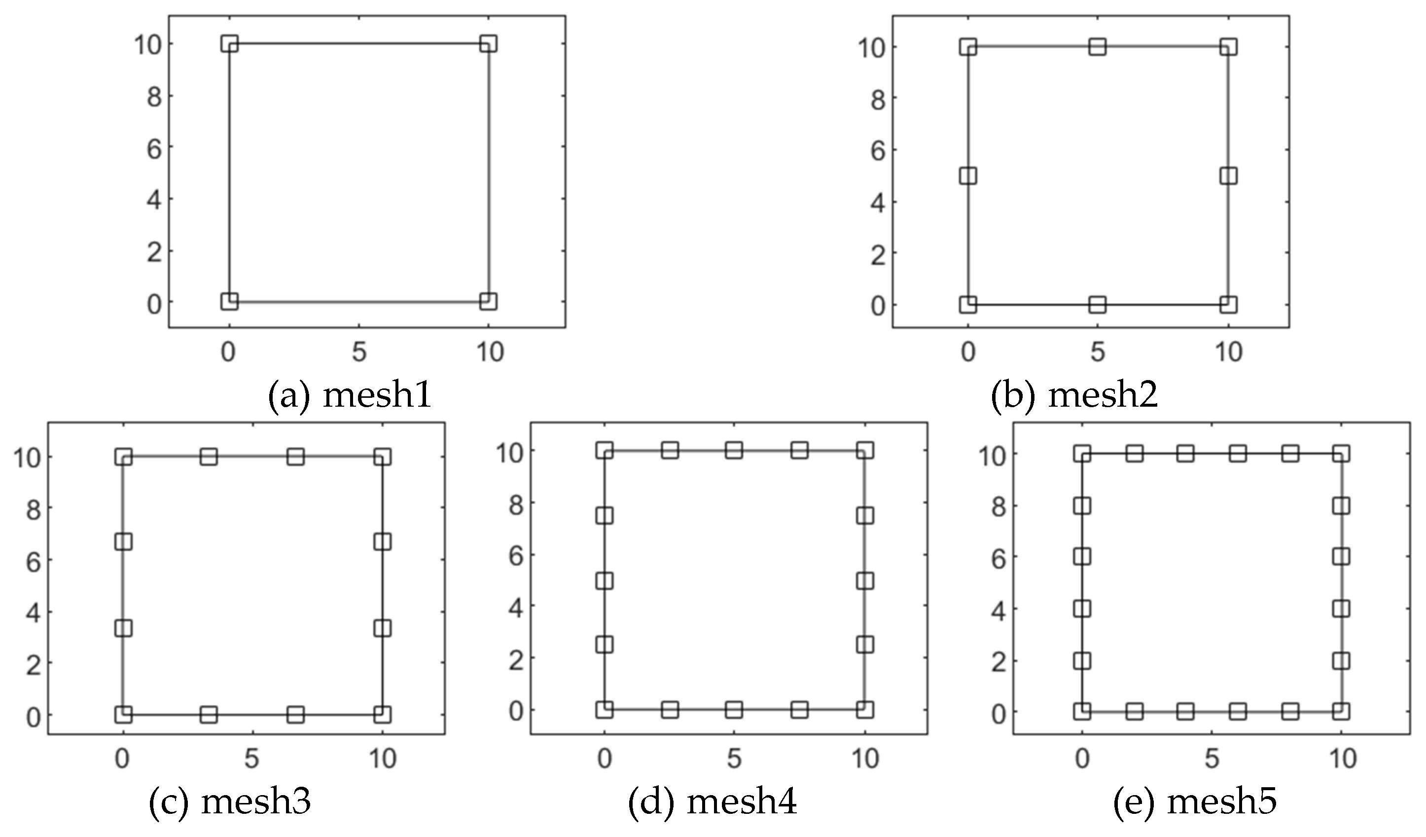
Figure 3.
The numerical errors of results of the plate under uniaxial tension calculated by the multi-patch WSIGABEM with collocation points generated by the improved Greville abscissae.
Figure 3.
The numerical errors of results of the plate under uniaxial tension calculated by the multi-patch WSIGABEM with collocation points generated by the improved Greville abscissae.
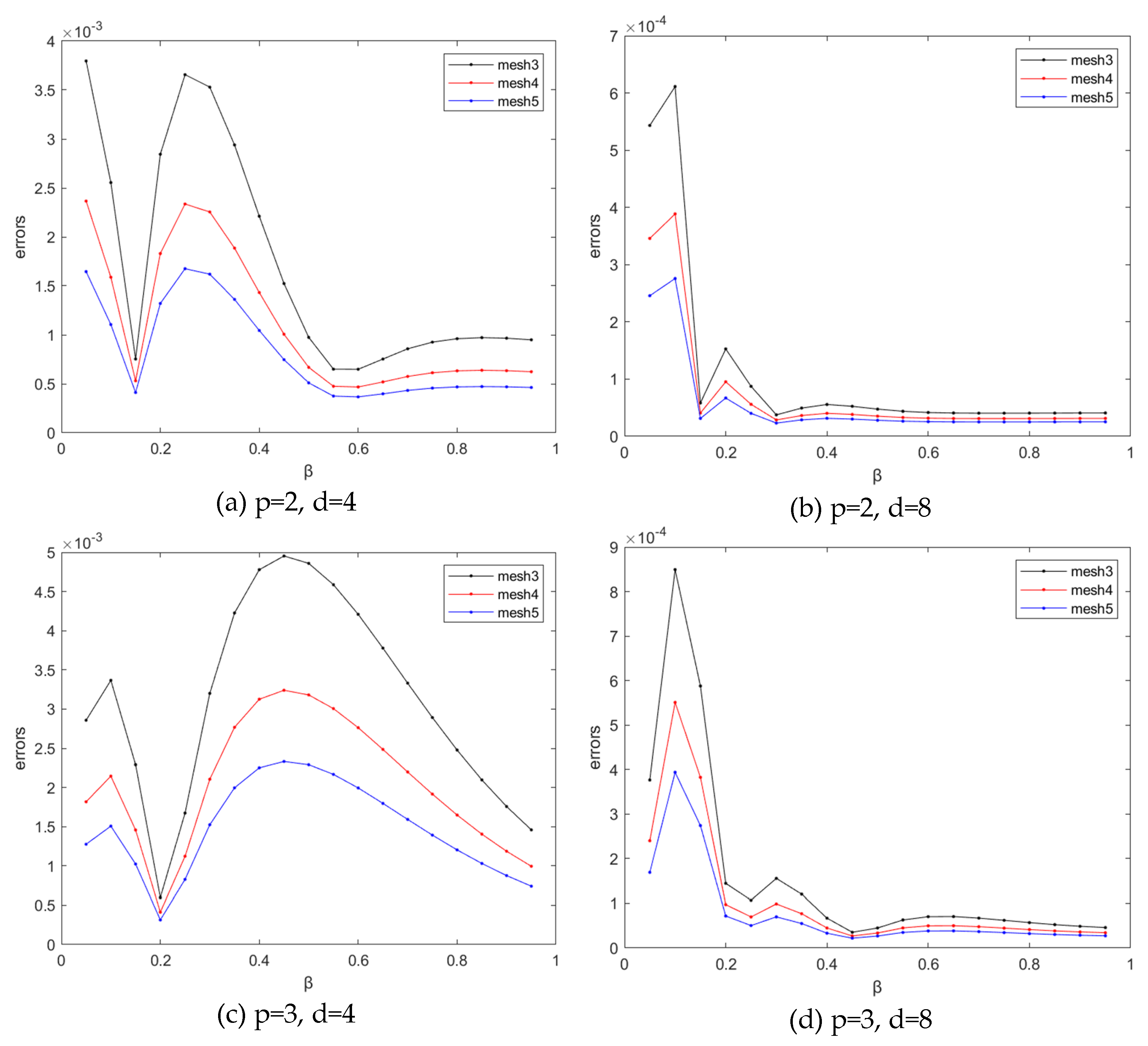
Figure 4.
Numerical Errors of the traditional IGABEM and the multi-patch WSIGABEM when the number of the Gauss points and the DOF are different.
Figure 4.
Numerical Errors of the traditional IGABEM and the multi-patch WSIGABEM when the number of the Gauss points and the DOF are different.
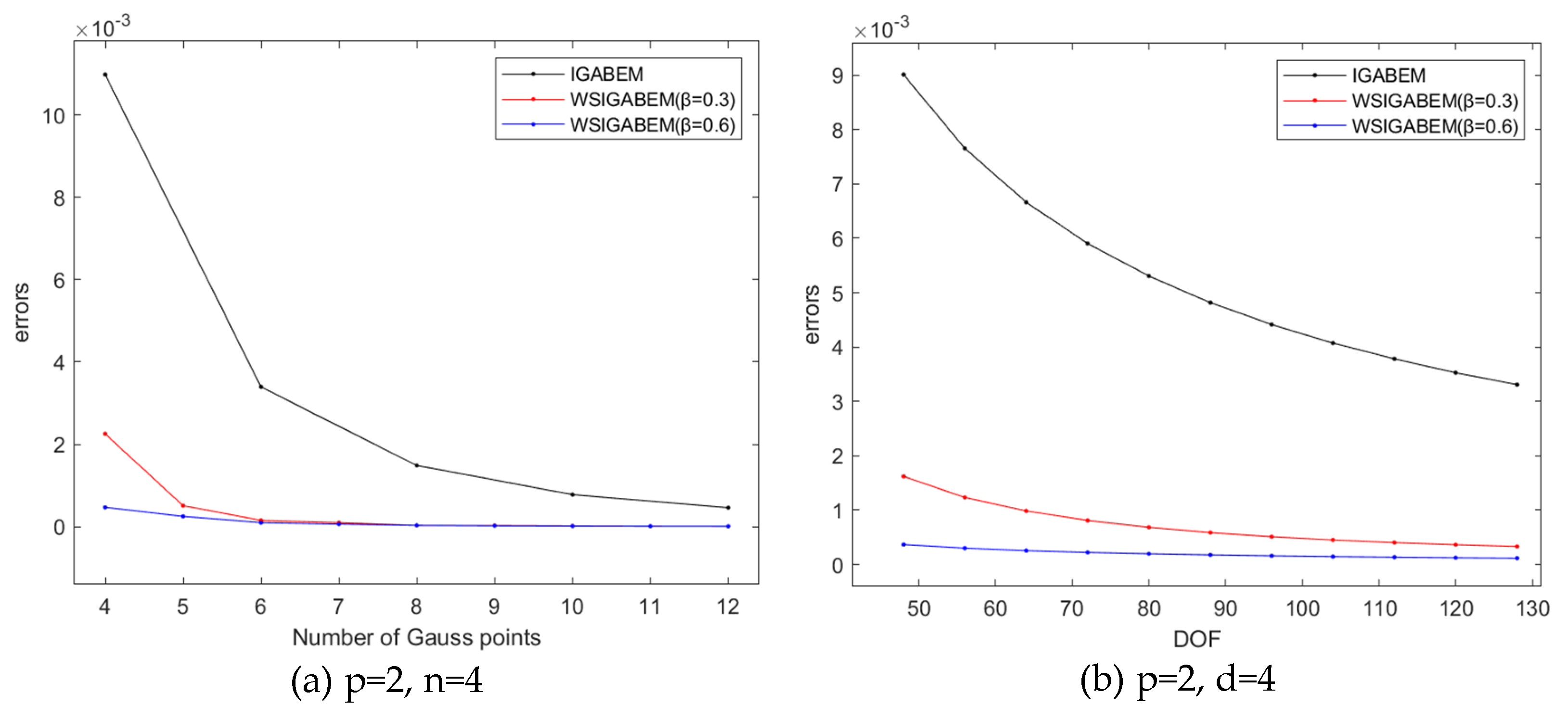
Figure 5.
Numerical Errors of the multi-patch WSIGABEM with different collocation point method when the number of the Gauss points and the DOF are different.
Figure 5.
Numerical Errors of the multi-patch WSIGABEM with different collocation point method when the number of the Gauss points and the DOF are different.
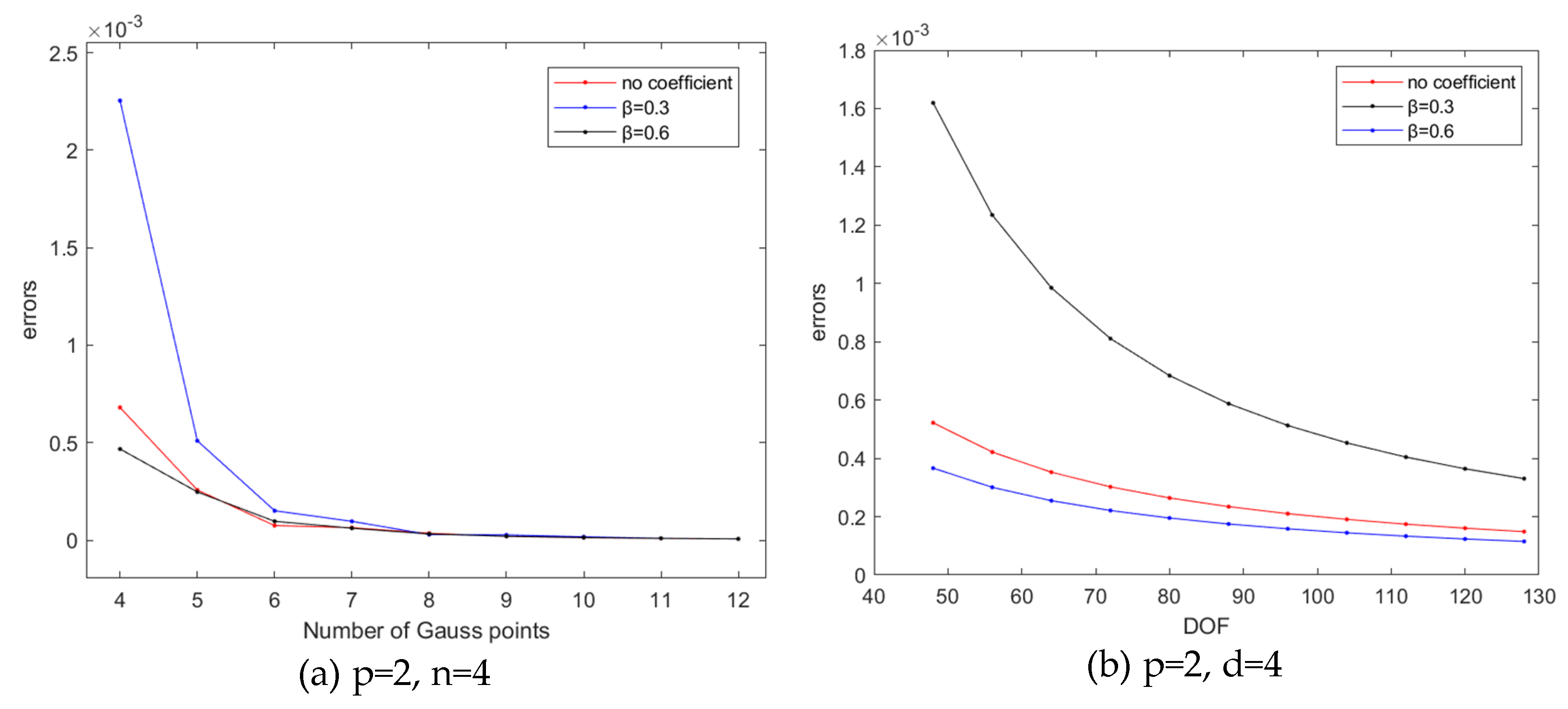
Figure 6.
An infinite plate with a hole under unidirectional stretching.
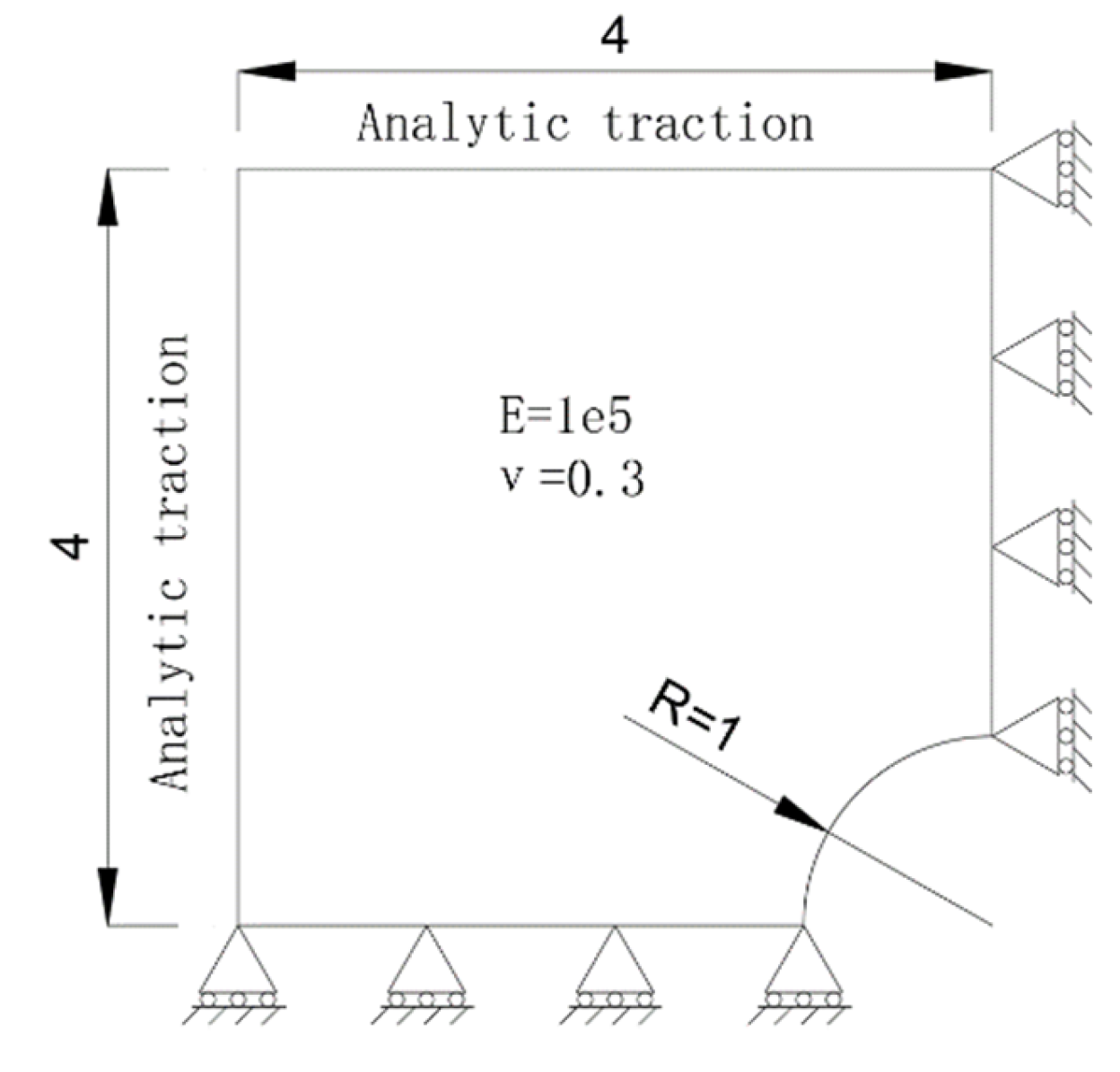
Figure 7.
Refinements of the model for the infinite plate with a hole under unidirectional stretching.
Figure 7.
Refinements of the model for the infinite plate with a hole under unidirectional stretching.

Figure 8.
The numerical errors of the multi-patch WSIGABEM with the improved collocation point method in different cases.
Figure 8.
The numerical errors of the multi-patch WSIGABEM with the improved collocation point method in different cases.
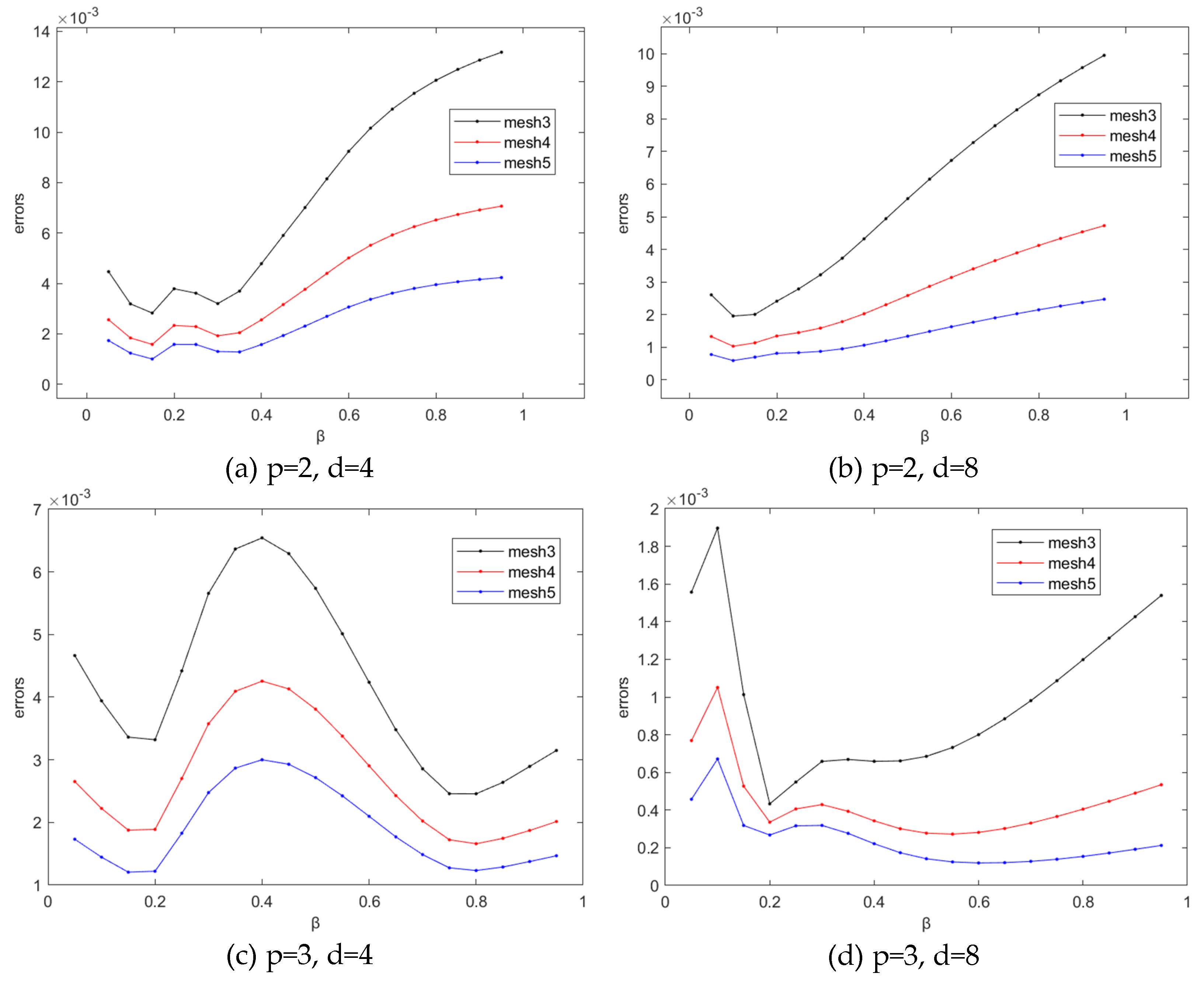
Figure 9.
Numerical Errors of the results of the infinite plate with hole calculated by the traditional IGABEM and the multi-patch WSIGABEM with the improved collocation point method when the number of the Gauss points and the DOF are different.
Figure 9.
Numerical Errors of the results of the infinite plate with hole calculated by the traditional IGABEM and the multi-patch WSIGABEM with the improved collocation point method when the number of the Gauss points and the DOF are different.
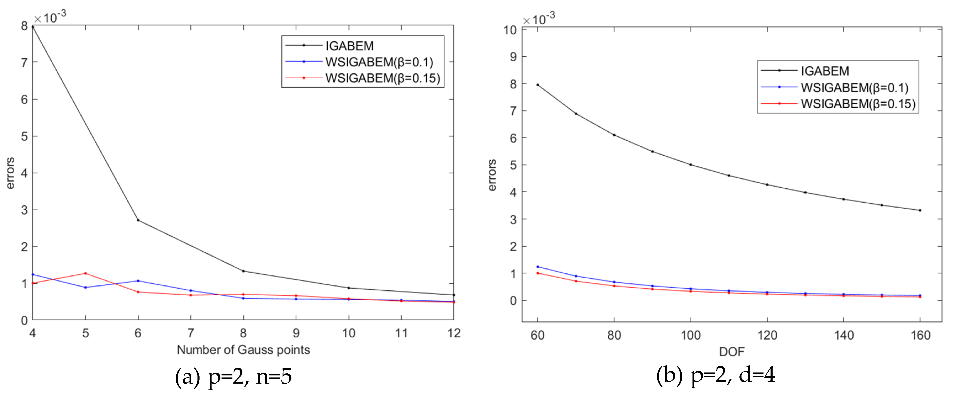
Figure 10.
Numerical Errors of the results of the infinite plate with hole calculated by the multi-patch WSIGABEM with different collocation point methods when the number of the Gauss points and the DOF change.
Figure 10.
Numerical Errors of the results of the infinite plate with hole calculated by the multi-patch WSIGABEM with different collocation point methods when the number of the Gauss points and the DOF change.
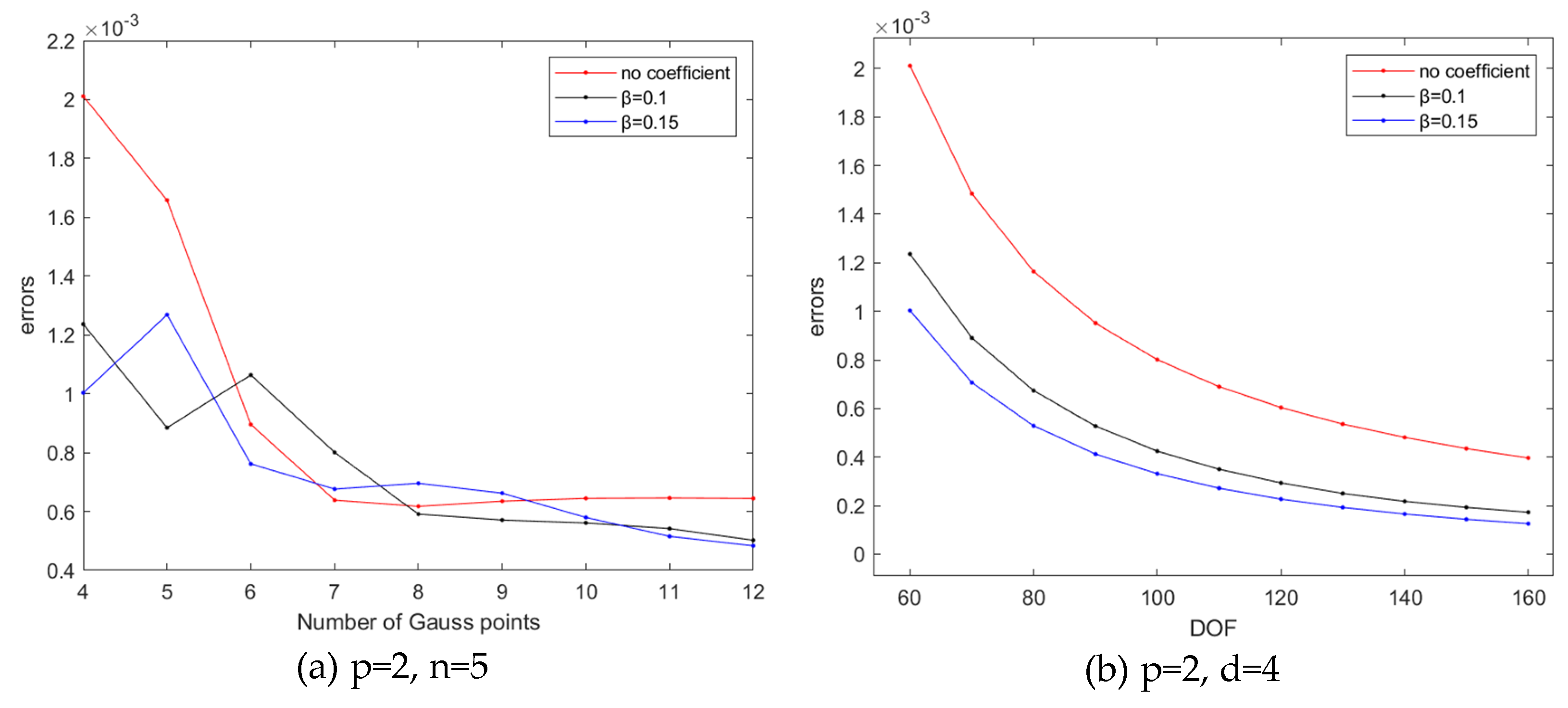
Figure 11.
Shape optimization of the fillet: (a) before the optimization; (b) after the optimization.
Figure 11.
Shape optimization of the fillet: (a) before the optimization; (b) after the optimization.
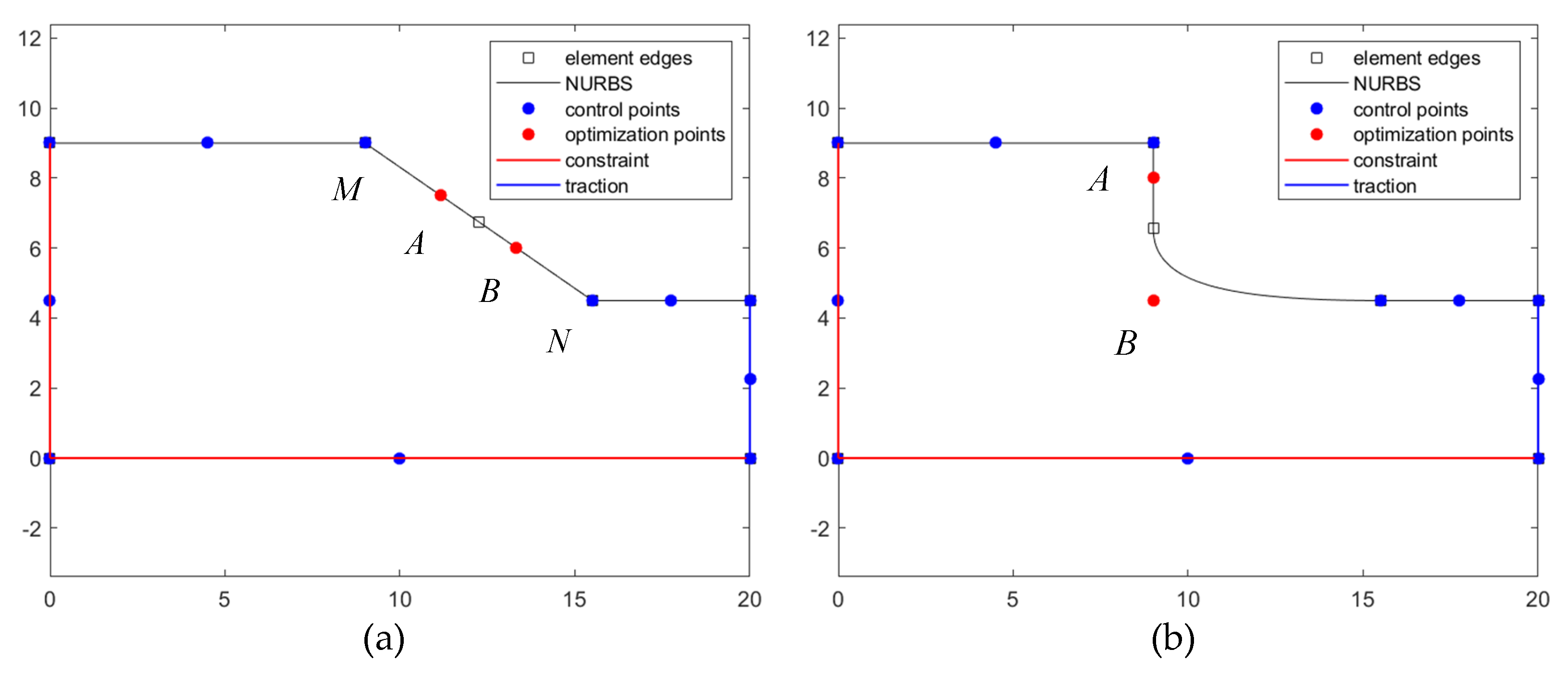
Figure 12.
The area of the fillet during the optimization.
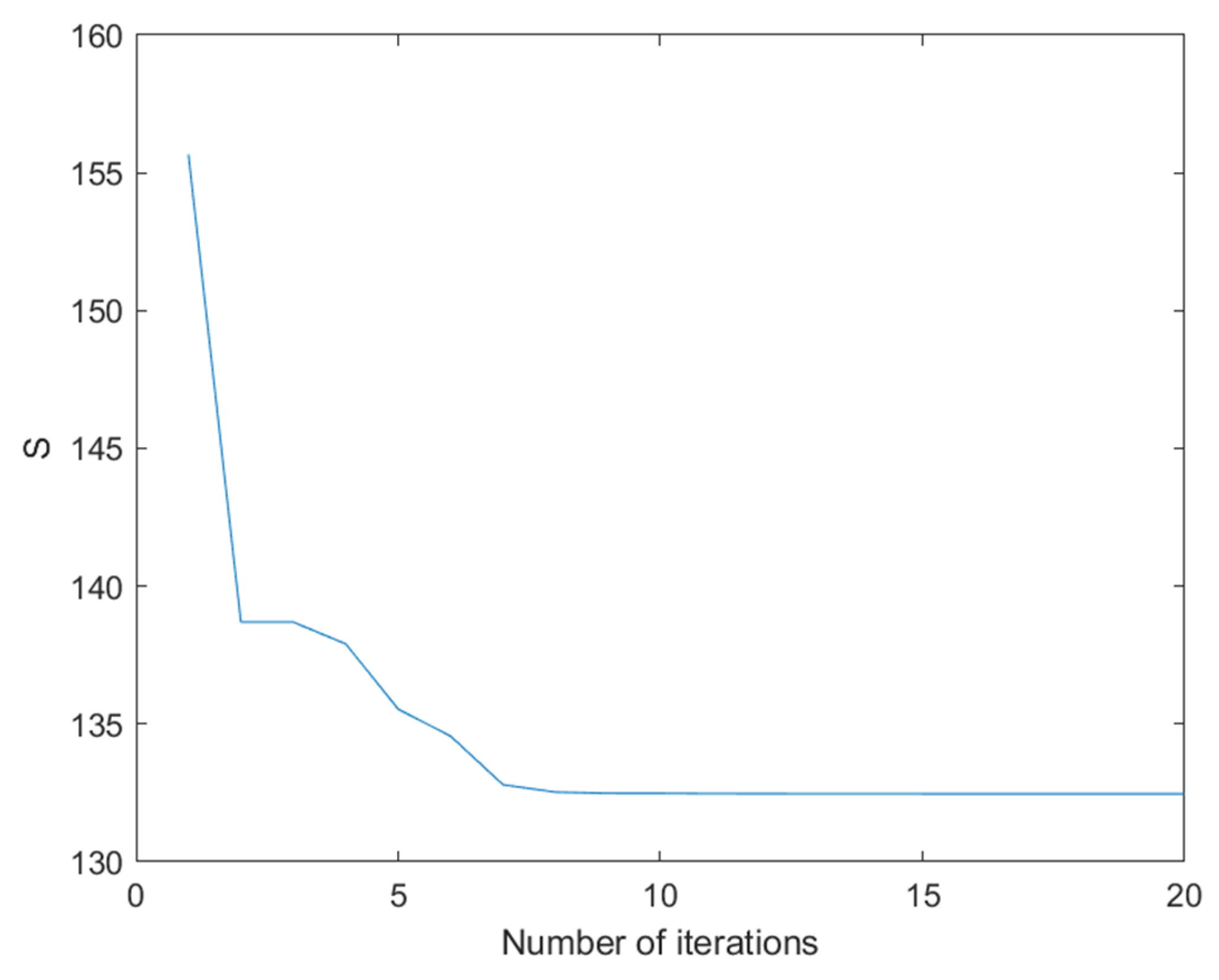
Figure 13.
Von Mises stress distribution on the boundary: (a) before the optimization; (b) after the optimization.
Figure 13.
Von Mises stress distribution on the boundary: (a) before the optimization; (b) after the optimization.
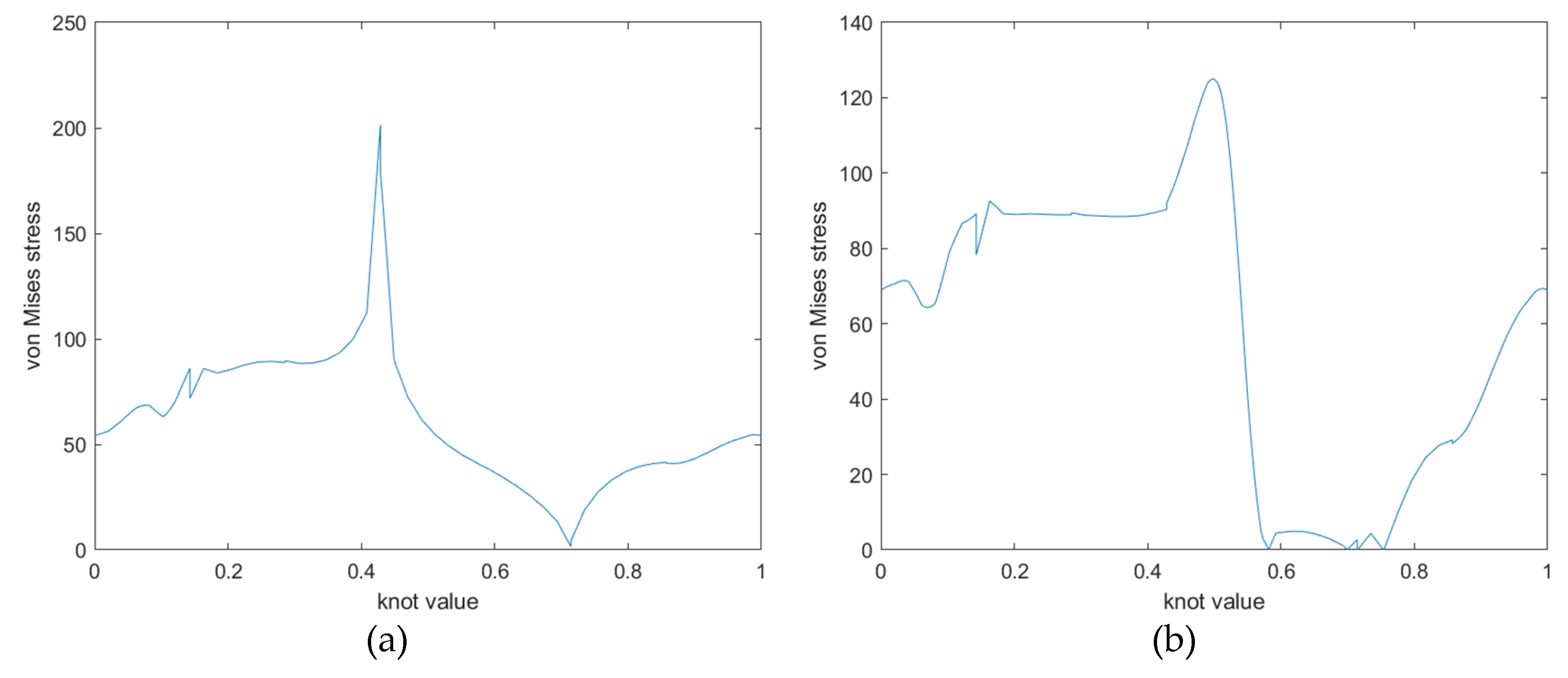
Figure 14.
The shape optimization of the spanner: (a) before the optimization; (b) after the optimization.
Figure 14.
The shape optimization of the spanner: (a) before the optimization; (b) after the optimization.
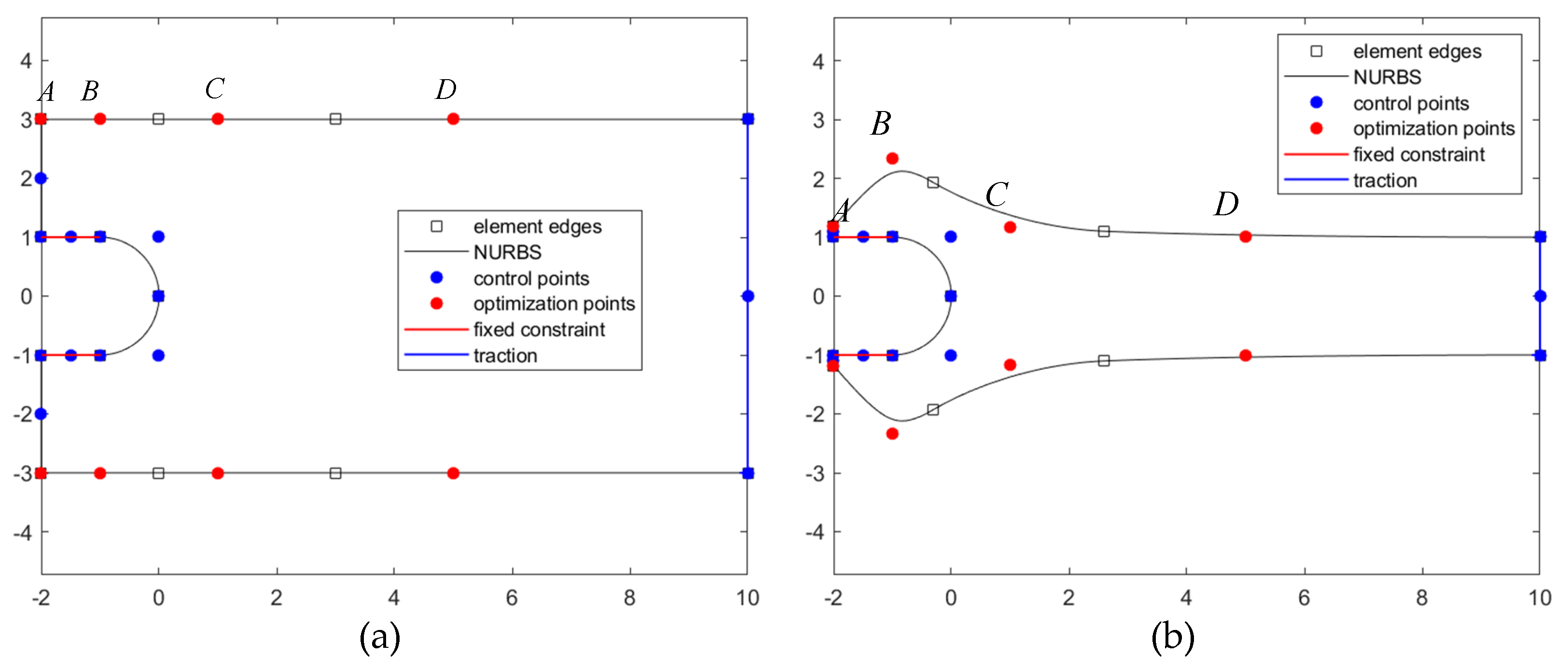
Figure 15.
The area of the spanner during the optimization.
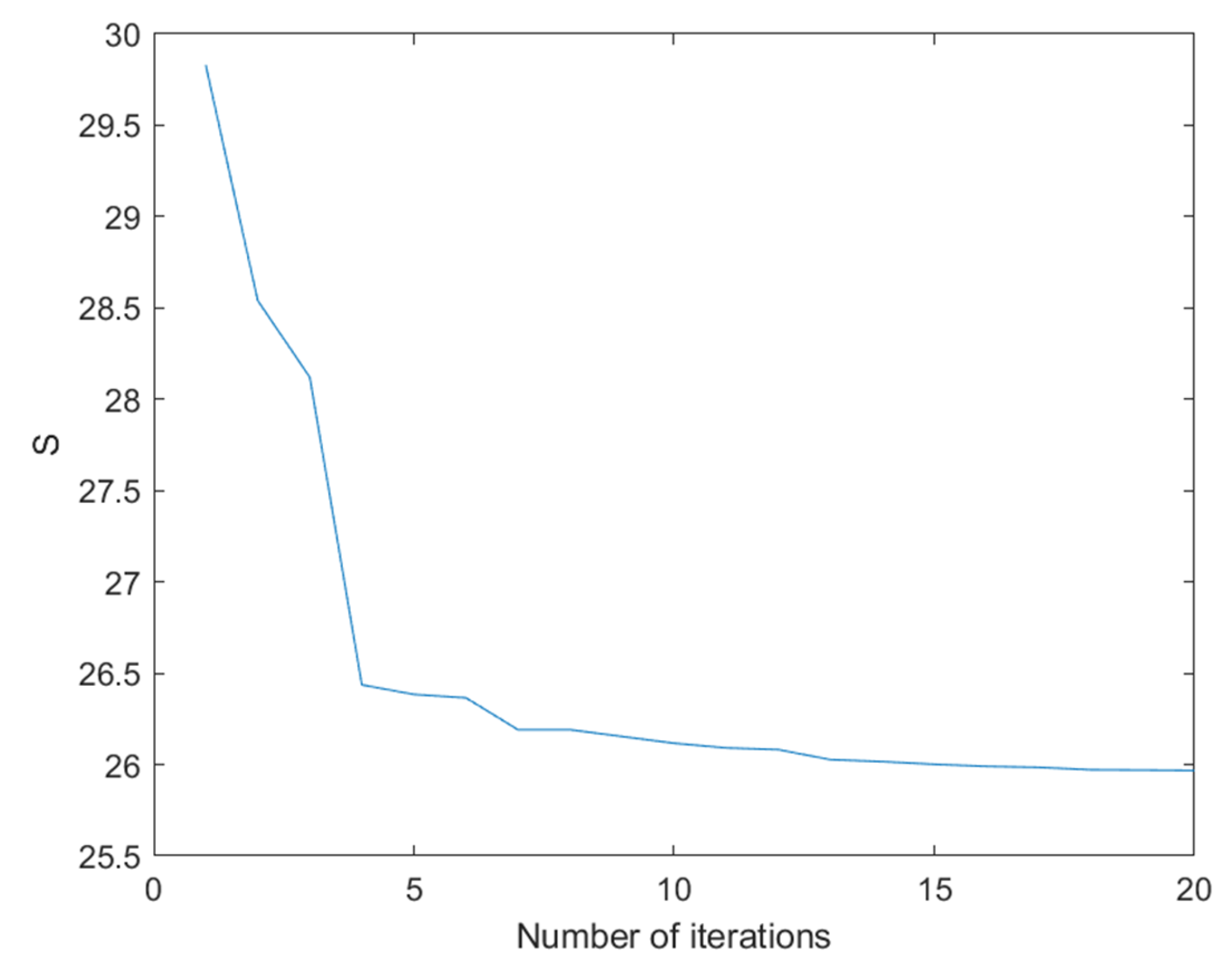
Figure 16.
The shape optimization of the arch bridge: (a) before the optimization; (b) after the optimization.
Figure 16.
The shape optimization of the arch bridge: (a) before the optimization; (b) after the optimization.
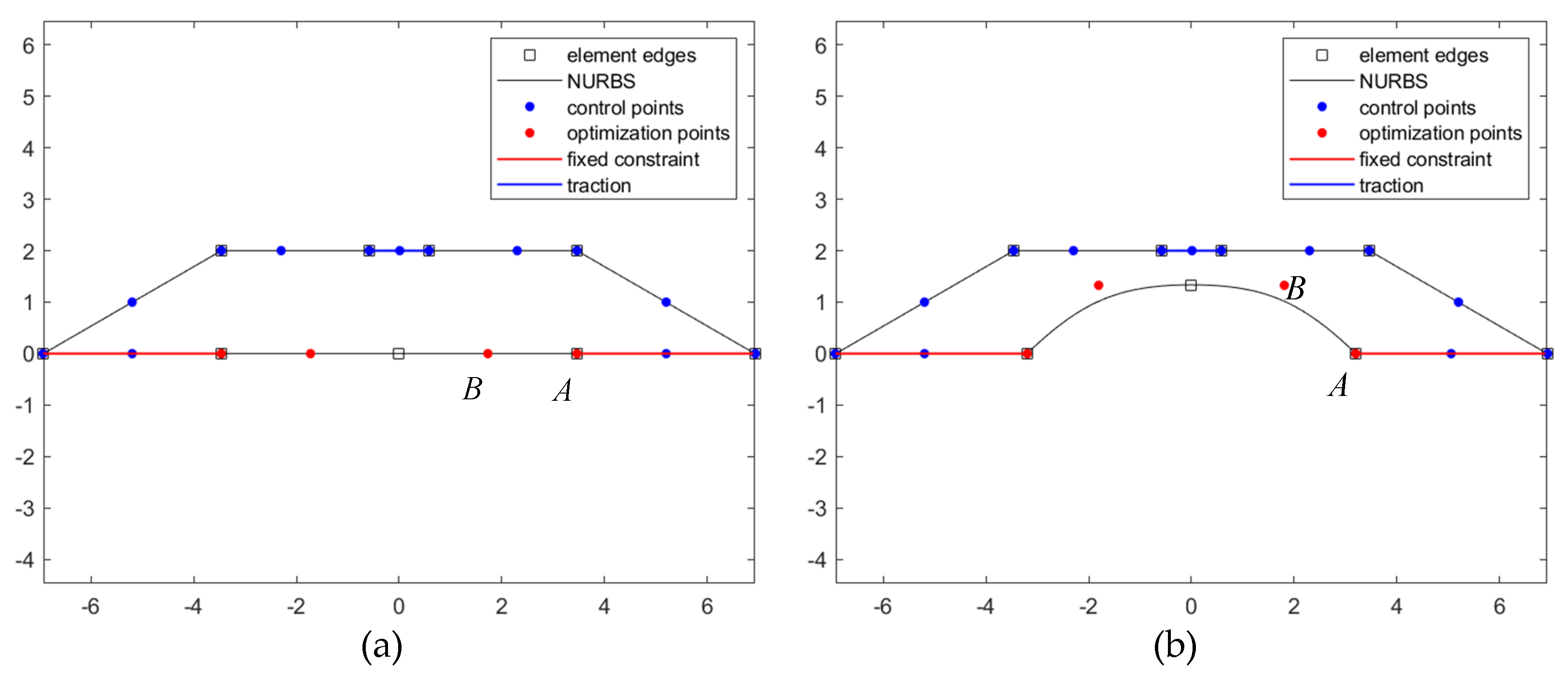
Figure 17.
The area of the arch bridge during the optimization.
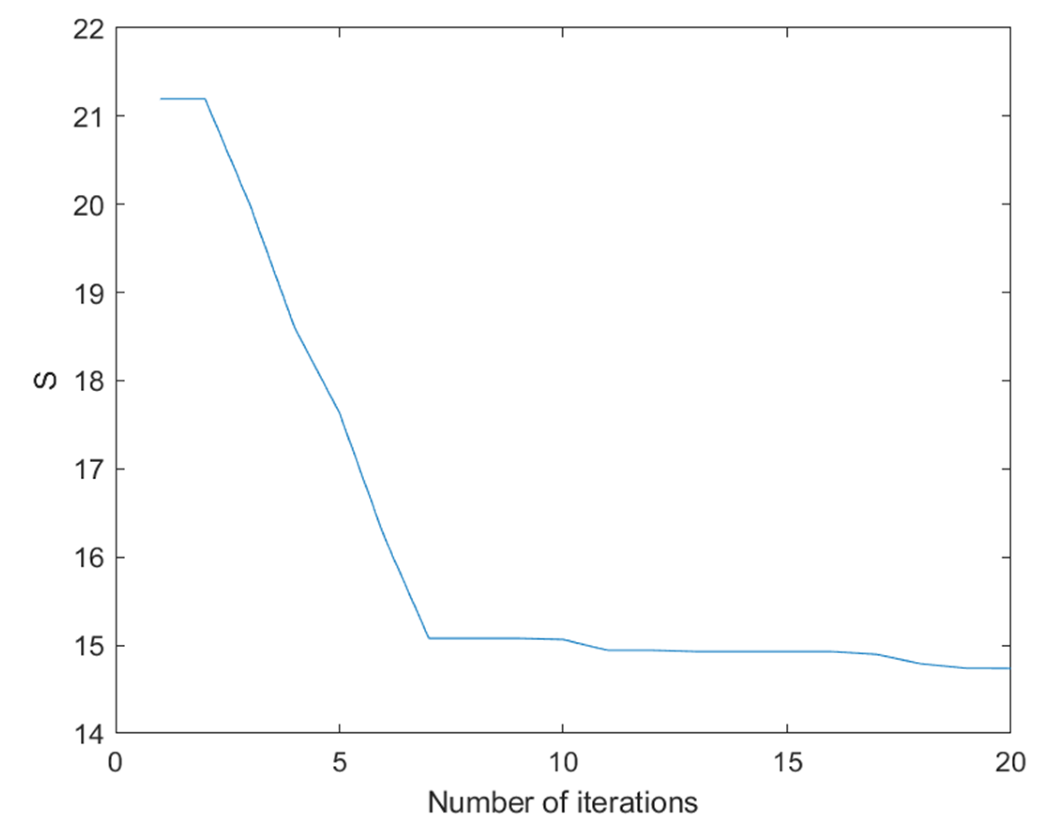
Table 1.
Algorithmic Principle Correspondence.
| Flock of Birds | PSO |
|---|---|
| Bird | Particle |
| Forest | Solution Space |
| Amount of food | Objective function value |
| Location of each bird | Particle position |
| The location with the most food | Global optimal solution |
Table 2.
The optimal correction coefficients for different d and n, when p = 2.
| p=2 | mesh3 | mesh4 | mesh5 |
|---|---|---|---|
| d=4 | 0.15 | 0.15 | 0.15 |
| d=8 | 0.1 | 0.1 | 0.1 |
Table 3.
The optimal correction coefficients for different d and n, when p = 3.
| p=3 | mesh3 | mesh4 | mesh5 |
|---|---|---|---|
| d=4 | 0.75 | 0.8 | 0.8 |
| d=8 | 0.2 | 0.55 | 0.6 |
Table 4.
The ranges and the values before and after the optimization of the design parameters for the shape optimization of the fillet.
Table 4.
The ranges and the values before and after the optimization of the design parameters for the shape optimization of the fillet.
| Design parameters | Lower bound | Upper bound | Before optimization | After optimization |
|---|---|---|---|---|
| A | (9, 4.5) | (15, 9) | (11.17, 1.5) | (9.00, 8.00) |
| B | (9, 4.5) | (15, 9) | (13.33, 6) | (9.00, 4.50) |
| wA | 0.1 | 10 | 1 | 2.49 |
| wB | 0.1 | 10 | 1 | 1.74 |
Table 5.
The ranges and the values before and after the optimization of the design parameters for the shape optimization of the spanner.
Table 5.
The ranges and the values before and after the optimization of the design parameters for the shape optimization of the spanner.
| Design variable | Lower bound | Upper bound | Before optimization | After optimization |
|---|---|---|---|---|
| A | (-2, 1.1) | (-2, 3) | (-2, 3) | (-2, 1.18) |
| B | (-1, 1) | (-1, 3) | (-1, 3) | (-1, 2.33) |
| C | (1, 0) | (1, 3) | (1, 3) | (1, 1.17) |
| D | (5, 1) | (5, 3) | (5, 3) | (5, 1.00) |
| wB | 0.1 | 10 | 1 | 2.93 |
| wC | 0.1 | 10 | 1 | 1.52 |
Table 6.
The ranges and the values before and after the optimization of the design parameters for the shape optimization of the arch bridge.
Table 6.
The ranges and the values before and after the optimization of the design parameters for the shape optimization of the arch bridge.
| Design variable | Lower bound | Upper bound | Before optimization | After optimization |
|---|---|---|---|---|
| A | (0,0) | (4, 0) | (2, 0) | (3.20, 0) |
| B | (0,0) | (2, 2) | (, 0) | (1.81, 1.34) |
| wB | 0.1 | 10 | 1 | 1.85 |
Disclaimer/Publisher’s Note: The statements, opinions and data contained in all publications are solely those of the individual author(s) and contributor(s) and not of MDPI and/or the editor(s). MDPI and/or the editor(s) disclaim responsibility for any injury to people or property resulting from any ideas, methods, instructions or products referred to in the content. |
© 2024 by the authors. Licensee MDPI, Basel, Switzerland. This article is an open access article distributed under the terms and conditions of the Creative Commons Attribution (CC BY) license (http://creativecommons.org/licenses/by/4.0/).
Copyright: This open access article is published under a Creative Commons CC BY 4.0 license, which permit the free download, distribution, and reuse, provided that the author and preprint are cited in any reuse.


