
Submitted:
05 February 2025
Posted:
06 February 2025
You are already at the latest version
Abstract
The Cauchy problem for the Laplace equation in an annular bounded region consists of finding a harmonic function from the Dirichlet and Neumann data known on the exterior boundary. This work considers a fractional boundary condition instead of the Dirichlet condition in a circular annular region. We found the solution to the fractional boundary problem using circular harmonics. Then, the Tikhonov regularization is used to handle the numerical instability of the fractional Cauchy problem. The regularization parameter was chosen using the L-curve method. From numerical tests, we found that the series expansion of the solution to the Cauchy problem can be truncated in N=20, N=25, or N=30. Thus, we found a stable method for finding the solution to the problem studied. To illustrate the proposed method, we elaborate synthetic examples and MATLAB programs to implement it. The numerical results show the feasibility of the proposed stable algorithm. In all cases, the solution with regularization gives better results than without regularization.
Keywords:
Cauchy problem
; Inverse problem
; Ill-posed problem
; Laplace equation
; Fractional boundary condition
; Tikhonov regularization
1. Introduction
The problem of determining a harmonic function defined in a bounded annular region from measurements on a part of the boundary (Cauchy data) is called the Cauchy problem for the Laplace equation [1]. It is well known that this problem is severely ill-posed in Hadamard’s sense, since small variations of the Cauchy data can produce large variations of the solution, i.e., the problem presents a numerical instability, implying that regularization techniques must be employed to solve it. To guarantee a solution to the Cauchy problem, some smoothness conditions must be imposed on the Cauchy data (see Theorem 1 in [2]).
The Cauchy problem is important because it has many applications, like estimating the deterioration of a pipeline, calculating a solution or potential in some regions or on boundaries where there is no direct access, and studying cracks on plates, [3,4,5]. Furthermore, the Cauchy problem is employed to study inverse electroencephalography and inverse electrocardiography [4,6,7,8,9,10].
There are different approaches to analyzing the Cauchy problem. In [11], the authors used the singular value decomposition to find the solution considering a circular annular region. Then, the admissible regularization strategy given by the spectral cut-off of the pseudo-inverse method was employed to handle the numerical instability of the problem. In [12] and [13], a new regularization method is proposed by applying the method of fundamental solutions to solve a Cauchy problem in an annular domain and a multi-connected domain, respectively. In [13], in order to effectively solve the discrete ill-posed problem resulting from a boundary collocation scheme, Tikhonov regularization, and L-curve methods were used to determine a stable approximate solution. In [11,14,15], and [16], the technique of layer potentials was used to obtain an equivalent system of integral equations. In [17], the Cauchy problem is resolved through a moment problem obtained using Green’s formula. This technique can be applied to annular regions that are more complex than circular ones. In [18], a similar technique is proposed for the 3-dimensional Cauchy problem, where the solution is expressed in terms of spherical harmonics and Tikhonov regularization is incorporated. In [19], a variational formulation of the problem was introduced, and the cost functional was minimized by conjugate gradient iterations, combined with a boundary element discretization of the state and adjoint equations. In [1], the potential on the interior boundary of the annular region is considered a control function, which must be determined for the potential on the exterior boundary to match the Cauchy input data adding to the cost function a penalized term that incorporates the Cauchy data. This allows determining the optimal solution using an iterative conjugate gradient algorithm. The computational cost of this algorithm is the solution to two elliptic problems per iteration, the state and adjoint equations, which are solved by the finite element method. A similar technique has been employed to solve other control problems, for instance, [9,10,19,20,21] and [22].
In this work, we consider one variant of the Cauchy problem. More precisely, we consider that we know the action of a fractional operator on the potential on the exterior boundary instead of the potential itself. We apply the Tikhonov regularization to handle the numerical instability that presents this variant, which we call the fractional Cauchy problem. Since we consider a circular geometry, we use the Fourier series method to solve the normal equations. The adjoint operator was found using its definition. From this, we found a stable algorithm for some of the parameters defining the fractional operator. To illustrate the results presented in this work, we elaborate synthetic examples and programs in MATLAB.
The paper is organized as follows: In Section 2, the definition and some results of the classical Cauchy problem, as well as the Sturm-Liouville operator, are presented. Section 2 also finalizes the definition of the fractional Cauchy problem. Section 3 applies the Tikhonov regularization to find an algorithm to recover the potential on the interior boundary. Section 4 presents numerical examples to illustrate the algorithm presented in this work. In section 5, we discuss the stability of the proposed algorithm. In section 6, we give the conclusions.
2. Problem Formulation
2.1. The Cauchy Problem
Let be a bounded annular region in with sufficiently smooth interior boundary and exterior boundary , as shown in Figure 1.
We consider the following boundary value problem: Find , such that
where , n is the outward unitary vector defined on , and denotes the outward normal derivative of w on . For simplicity, we consider (1) with by the change of variable , where is the unique harmonic function satisfying on , and . Then
where . For the analysis of the Cauchy problem (2) the following problem is employed (see [3,15]):
Given a function φ defined on , find u such that
This problem is well-posed, and we will call it the auxiliary problem.
The inverse problem associated with the Cauchy problem can be formulated in the following way:
Recover the potential on from the measurements on , where u is the solution to the auxiliary problem (3).
Definition 1.
A function is a weak solution to the auxiliary problem (3) if
where
Theorem 1 given in [1] guarantees the existence and uniqueness of the weak solution, and allows us to define the lineal, injective, and compact operator that associates to each the trace over of the weak solution u to the auxiliary problem (3). Operator K is compact because it is the composition of the continuous operator , which associates to each the weak solution to the auxiliary problem (3), with the trace operator from into , which is compact. The relationship between problem (2) and auxiliary problem (3) can be described by the operator K as follows:
A solution to the auxiliary problem (3) is also a solution to the problem (2) if we choose φ on , such that
where denotes the solution to the auxiliary problem (3), and V is the known measurement in problem (2), so we have .
The following result is very important for the statement of the minimization problem presented in Section 3 and its demonstration can be found in [19].
Theorem 1.
is dense in .
Equation (7) does not have a solution for all . However, if we impose some smoothness conditions on V, we can find global conditions of the existence of the solution, as in [19]. As K is an injective and well-defined ([3]) operator, it ensures uniqueness when a solution is available. Since the operator K is lineal, injective, and compact, its inverse is not continuous. Therefore, the inverse problem is ill-posed due to its numerical instability.
2.2. Sturm-Liouville Operator
The following material has been obtained from [23]. Let be a unit ball, . The corresponds with the unit sphere; , let be a Dirac operator, where . Let be a smooth function on the domain . For any the following expression
is called an operator of integration of the order in the Hadamard sense. Furthermore, we will assume that
We consider the following modification of the Hadamard operator:
where m is a positive integer.
Properties and application of the operators y have been studied in [23]. In that paper, the authors studied a certain generalization of the classical Neumann problem with the fractional order of boundary operators. Let , . In the domain the authors consider the following problem:
2.3. Fractional Cauchy Problem
We consider the following fractional Cauchy problem
where the operator is given in (9).
For the analysis of the fractional Cauchy problem (12), also we consider the auxiliary problem (3). We define the operator , which is a compact operator. We have the following two definitions to study the problem that concerns us.
Definition 2.
The Forward Problem (FP) related to the fractional Cauchy problem consists of finding the potential when φ is known.
Definition 3.
Given , the Inverse Problem (IP) related to the fractional Cauchy problem consists of finding such that .
3. Methods
3.1. Tikhonov Regularization of the Fractional Cauchy Problem
To find an approximate solution of equation (7) for when we have measurement with error , the minimization of the following Tikhonov functional is proposed in [24]:
where is the Tikhonov regularization parameter, which will be chosen by the L-curve method. It is proved that J is strictly convex and twice Frechet differentiable, so it has a unique minimum in . This least squares procedure is equivalent to solving the normal equation
where is the adjoint operator.
Given , the exact solution to the auxiliary problem (3) in a circular annular region , in polar coordinates, is given by:
where . The values , , are the Fourier coefficients of . The solution to the FP, called measurement, is given by , which is obtained by applying of the operator , the identities:
, ,
, ,
and then evaluating in , i.e.,
where the Fourier coefficients of exact measurement V are given by , for , 2, in which
In the numerical examples, the integrals are calculated using the function quadl of MATLAB.
The `exact solution’ u and the `exact measurement’ are generated taking terms of the Fourier series (15) and (16), with , which is obtained from numerical tests. To find the solution to the IP, we must solve the normal equations. To do this, we calculate the adjoint operator using its definition:
Without loss of generality, we consider functions in which the constant term of their series expansion is null. Using (16) and (18) we found
Thus, the adjoint operator is defined by ,
3.2. Tikhonov Regularization for the Classical Cauchy Problem
Given , the exact solution to the auxiliary problem (3) in a circular annular region is given, in polar coordinates, by (15). Therefore, the measurement is obtained with in (15):
which is the solution to the FP. The Fourier coefficients of V are given by
Therefore, the solution to the IP from the measurement with error
is given by the regularized solution
where
where are the Fourier coefficients of and is the Tikhonov regularization parameter. Thus, the solution to the IP (of the classical Cauchy problem) applying the Tikhonov regularization method (TRM) is given by (15) replacing the coefficients by the coefficients given by (25).
4. Numerical Results
In this section, we illustrate the method proposed in this work using synthetic examples. We know the exact defined on in this case. Then, we calculated the measurement with and without noise by solving the FP for the classical and fractional Cauchy problem.
The exact measurement is calculated by solving the FP. To generate the measurements with error , we added to the exact measurement a Gaussian error using the function of MATLAB. The exact measurement was calculated by solving the FP. Therefore, we define
where is a vector of random numbers of length m (numbers of nodes on ) with a normal distribution. The corresponding numerical solutions are denoted by .
In this section, we obtain the relative error between the exact source and the recovered source shown in Tables and denoted by . The relative error is given by
and the relative error between the exact measurement V and the measurement with error are denoted , which is given by
where is the norm of the space .
4.1. Solution to the IP Related to the Classical Cauchy Problem
In the following two examples, we consider a circular annular region with and , then and are two circumferences of radii and (see Figure 1), respectively.
Example 1. We take the `exact potential’ , , that in polar coordinates is . In this case, , and the solution to the forward problem, that is, the solution to the auxiliary problem (3), is given by
where . Then the `exact solution’ V and the `measurement with error’ are generated with the first N terms of the Fourier series (22) and (23), respectively. In this case, we take values of , 25, and 30 terms. Therefore, the measurement with error is given by the series
where are the Fourier coefficients of . The regularized solution to the inverse problem is given by the series (24) truncated to N terms. The solution without regularization to the IP is given by
where the coefficients are given by
Remark 1: In all Tables associated with the classical case, if , then the solution is the solution without regularization given by (28), where the coefficients are given by (29).
Table 1 shows the numerical results for data with and without error, applying TRM to solve the IP of the classical Cauchy problem (2). In this case, we observe that the solutions with regularization have a percentage of relative errors around equal to the percentage of error including in the data with error for . The regularization parameter was chosen as , for , 25, and 30. Also, we can see that the decrease when the error tends to zero, while the increases for each value of N. In particular, the increases faster when , for , , y . In this case, the regularization parameter depends on .
Figure 2(a) and Figure 2(b) show the graphs of the exact measurement V and with error , the graphs of the exact potential and its approximations (with regularization) and (without regularization) taking and , corresponding to the Example 1, for (see Table 1). In Figure 2(b), we can see the ill-posedness of the inverse problem if we do not apply regularization, where and .
Example 2. We consider the `exact potential’ , for . Similar to the first example, the `exact measurement’ V and the `measurement with error’ are generated with the first N terms of the Fourier series (22) and (23), respectively, such that , with . In this case, and the Fourier coefficients , are obtained numerically using the intrinsic function of . Here, we take values of , 25 and 30 terms.
Table 2 shows the numerical results for data with and without error, applying TRM to solve the IP of the classical Cauchy problem (2). Analogous to Example 1, we can observe that the solutions with regularization have a percentage of relative errors around equal to the percentage of error including in the data with error for . Also, we can see that the decrease when the error tends to zero, while the increases for each value of N. In particular, the increases when for each , , and . As in the previous example, the regularization parameter depends on , and we take for each value of , 25 and 30.
Figure 3(a) and Figure 3(b) show the graphs of the exact measurement V and with error , the graphs exact potential and its approximations (with regularization) and (without regularization) taking and , corresponding to the Example 2, for (see Table 2). In Figure 3(b), we can see the ill-posedness of the inverse problem if we do not apply regularization. In this case, and .
4.2. Solution to the IP Related to the Fractional Cauchy Problem
In this section, we look into the performance of the TRM to solve the IP of the fractional Cauchy problem (12), in a circular annular region with and , then and are two circumferences of radii and (see Figure 1), respectively. In this case, we consider as `exact potentials’ the two functions from the previous Subsection: , and , for .
Similar to the previous subsection, the `exact solution’ V and the `measurement with error’ are obtained by truncating the series (16) and (23) up to N terms, respectively, furthermore, the Fourier coefficients , and (given by (17)) are obtained numerically using the function of .
In this case, we take values of , 20, 25, and 30 terms. Therefore, the measurement with error is given by the series (23) truncated to N terms. The regularized solution to the IP is given by the series (21) truncated to N terms. Also, the solution without regularization to the IP is given by (28), where
Remark 2: In all Tables from fractional case, if , the solution is the solution without regularization given by (28), where the coefficients are given by (30).
4.2.1. Case 1: and , When Tends to Zero
In this section, we consider the case when , , and for different values of close to zero. Table 3 and Table 4 show the relative errors of the approximations and , when tends to zero, for the two exact functions considered in the SubSection 4.1. In both cases, we observe that the of the solutions with regularization are less than the , for each value of and N given in these Tables. Additionally, the and are of the same order, i.e., the solutions without regularization are close to regularized solutions , for and . In both cases, the measurements with errors do not have much impact on recovered solution , and they are close to . We observe from the relative errors that regularized approximations are better than those without regularization. In this case, the regularization parameter depends on , N, m and .
Considering , , and , we show the graphs for the following potentials (Figure 4), and (Figure 5), for , where:
- (a)
- The exact measurement V and the measurement with error .
- (b)
- The exact potential and its approximations (with regularization) and (without regularization) taking and .
4.2.2. Case 2: , for and .
Table 5 and Table 6 show that the relative errors of the approximations and when , for the two exact functions considered in the SubSection 4.1.
In Table 5, we observe that for each value of N, and m given in the mentioned Table. Also, the and are of the same order, i.e., the solutions without regularization are close to regularized solutions , for , , 25, 30, and . We can see similar results in Table 6 for , , 25, 30, , , and , 3, however the regularized approximates are better than the solutions without regularization. Furthermore, and these increase suddenly, starting in and (see Table 5 and Table 6) for the functions and for , respectively. As in the previous case, the regularization parameter changes depending on , N, m, and .
We show the graphs for the following functions:
- (Figure 8, with parameters , , , , and ),
for . These Figures show:
- (a)
- The exact measurement V and the measurement with error .
- (b)
- The exact potential and its approximations (with regularization) and (without regularization).
In both cases, as mentioned in the previous paragraph, the errors increase suddenly, starting in for the first function and for the second one, as can be seen in Figure 7(b) and Figure 8(b), where we can see the ill-posedness of the IP if we do not apply regularization. For example, for the second function, the is much greater than , for , and (see Table 6). However, in this same example, for , 10, 11, and 12 the increases around 90%. Nevertheless, is bigger than . In this case, we could use the regularized solution as an initial point of an iterative method to recover a better solution to the IP.
4.2.3. Case 3: , when is next to or m and .
This Section considers the case when and is next to or m. Table 7 and Table 8 show that the relative errors of the approximations and when for the same two exact functions considered in SubSection 4.1.
In Table 7, we observe that the are less than the , for each value of N, and m given in this Table. We can see that and are of the same order for , 2, i.e., the solutions without regularization are close to regularized solutions . However, the regularized approximates are better than the solutions without regularization, for , 2. Nonetheless, the increases more than starting in . Furthermore, we can observe similar results in Table 8 where the are less than the , for , 2, 3, 4, with , , and the different values of are close to m or given in this Table. For the values of , 6, 7 and 8, the are around the percentage of the . For the other values of , 10, 11 and 12, given in Table 8, the corresponding increases around 90%, but no more than , i.e., the TRM does not provide a good approximate solution to the IP. In this case, we could use the regularized solution as an initial point of an iterative method to recover a better solution to the IP. Besides, the relative errors of the recovered solutions without applying regularization increase suddenly, starting in and (see Table 7 and Table 8) for the functions and for , respectively. As in the previous cases, the regularization parameter changes depending on , N, m and .
We show the graphs for the following functions:
for . These Figures show:
- (a)
- The exact measurement V and the measurement with error .
- (b)
- The exact potential and its approximations (with regularization) and (without regularization).
In both cases, as mentioned in the previous paragraph, the errors increase starting in for the first function and starting in for the second one, as can be seen in Figure 9(b) and Figure 10(b) for , where we can see the ill-posedness of the IP if we do not apply regularization. For example, for the first function, the is greater than , for , and (see Table 7). For the second one, the is greater than , for , and (see Table 8). In this latter function, the approximate solution is far from the exact solution . In this case, we could apply an iterative method to obtain a better solution, taking as an initial point.
4.2.4. Case 4: , for ,...,12 and .
In this Section, we consider the case when for , 3,...,12 and . Table 9 and Table 10 show that the relative errors of the approximations and when , with the same two exact functions considered in the SubSection 4.1.
In Table 9, we observe that the from solutions with regularization are less than the . For some values of N, and m given in this same Table, we can see that and are of the same order, i.e., the solutions without regularization are close to regularized solutions , however the regularized solutions are better than the solutions without regularization. The increases faster than the starting in . Furthermore, we can observe similar results in Table 10 where the are of the same order than , for , 3, 4, with , , except for . Nevertheless, the increases faster than the starting in . For the values of , 9 10, 11, and 12, the increases between 40% and 90%, but no more than . In this case, the TRM does not provide a good approximate solution to the IP. However, as mentioned before, we could use the regularized solution as an initial point of an iterative method to recover a better solution to the IP. Also, the relative errors of the recovered solutions without applying regularization increase suddenly, starting in and (see Table 9 and Table 10) for the functions and for , respectively. Here also, as in the previous cases, the parameter of regularization changes depending on , N, m and .
Figure 11 and Figure 12 show the graphs of the exact measurement V and with error with , the graphs exact potential and its approximations (with regularization) and (without regularization), corresponding the functions and for , respectively. In both cases, as mentioned in the previous paragraph, the errors increase suddenly, starting in for the first function and starting in for the second one, as can be seen in Figure 11(b) and Figure 12(b), where we can see the ill-posedness of the IP if we do not apply regularization. For example, for the first function, the relative error is greater than , for , y (see Table 9). For the second one, the is greater than , for , and (see Table 10). In this case, we could use the regularized solution as an initial point of an iterative method to recover a better solution to the IP.
4.2.5. Case 5: , when is next to n or , where , for and .
In this Section, we consider the case when , when is next to n or , where , for and . Table 11 and Table 12 show that the relative errors of the approximations and when , for the same two exact functions considered in the SubSection 4.1.
In Table 11, we observe that . For , we can see that and are of the same order when is next to 1 or 0 (taking ), i.e., the solutions without regularization are close to regularized solutions . However, the regularized approximates are better than the solutions without regularization. The increases faster than the starting in , as shown in Figure 13(b) for , and , where and . These approximations and are recovered from measurements with error , shown in Figure 13(a). Also, we can observe similar results in Table 12 where and are of the same order for , 3, 4, and when is next to n or (taking , 1, and 3, respectively), for , nevertheless the increases between 17% and 38% but no more than the for , 6, 7, and 8. For the values of , 10, 11, and 12 the increases around 90%, but no more than . In this case, we could use the regularized solution as an initial point of an iterative method to recover a better solution to the IP. Nevertheless, the relative errors of the recovered solutions without applying regularization increase suddenly, starting in and (see Table 11 and Table 12) for the functions and for , respectively. Here, the regularization parameters also change depending on , N, m and .
Figure 13, Figure 14, Figure 15 and Figure 16 show the graphs of the exact measurement V and with error with , the graphs of the exact potential and its approximations (with regularization) and (without regularization), corresponding to the functions and for , respectively. In both cases, as mentioned in the previous paragraph, the errors increase suddenly starting in for the first function and starting in for the second one, as can be seen in Figure 14(b), Figure 15(b) and Figure 16(b), where we can see the ill-posedness of the IP if we do not apply regularization for , 8 and , respectively. For example, for the approximations and shown in Figure 14(b) of the first function, the is much greater than , for , and (see Table 11). For the approximations and shown in Figure 15(b) of the second one, the is much greater than , for , y (see Table 12). Lastly, for the approximations and shown in Figure 16(b) of the second one, the is greater than , for , and (see Table 12). In these last two examples, when the approximate solutions are not close to the exact solution , we could use the regularized solution as an initial point of an iterative method to recover a better solution to the IP.
4.2.6. Case 6: , for ,...,13 and .
In this case, we consider the case when , with for . Table 13 and Table 14 show that the relative errors of the approximations and when , for the same two exact functions considered in the SubSection 4.1.
In Table 13, we observe that . For , we can see that and are of the same order when , i.e., the solutions without regularization are close to regularized solutions . However, the regularized approximates are better than the solutions without regularization. Additionally, the relative errors of the solutions without regularization increase faster starting in . Furthermore, we can observe similar results in Table 14. In this case, the relative errors from solutions with regularization are less than the for , and increase between 29% and 46% for , when . Nevertheless, the corresponding relative errors of the solutions with regularization increase between 88% and 96% for , but no more than the corresponding . The relative errors of the recovered solutions without regularization increase suddenly, starting in . For example, for and the . For , the increases between 91% and 99%, but no more than the ), for , as well as for and with . Moreover, as in the previous cases, the regularization parameters change depending on the data with error , the values N, m, and . Analogous results can be obtained for values , as those obtained for , which are not included in this work.
5. Discussion
The numerical tests show that the proposed algorithm usually gives good results. Even if the numerical results are unsatisfactory, they are enough to start an iterative method. In all cases, the regularized method is worth more than the method without regularization. After some numerical tests, we found that the series expansion of the solution to the fractional Cauchy problem can be truncated in , , or .
When for , the results obtained are similar, i.e., the results obtained with and without regularization almost coincide. One possible explanation can be associated with the smoothing properties of the integral operator to have similar results when , for . In the other cases, the regularized case is better.
When , the regularized method loses precision. However, the approximate solution obtained can be used as an initial point of a stable iterative method. From the numerical results, we want to emphasize that the solution by the Tikhonov regularization method of the classical Cauchy problem works adequately in all cases.
The Tikhonov regularization parameter, which was chosen by the L-curve method, was very large in some cases. We do not have an explanation for this situation, but we consider this an interesting topic that must be studied in future works.
In the classical Cauchy problem, the adjoint operator is associated with a boundary value problem called the adjoint problem. In the fractional Cauchy problem, we calculate the adjoint equation operator using its definition. One interesting question is whether a boundary value problem is associated with the adjoint operator. If the answer is positive, the following question arises: Can the adjoint operator be used in irregular regions?
6. Conclusions
This work proposes an algorithm to solve the fractional Cauchy problem obtained from the Tikhonov regularization and the circular harmonics. The numerical results show that the algorithm is feasible for various parameters. In some cases, despite not being a good approximation, the regularized solution is much better than the solution without regularization. So, the solution that delivers the algorithm can be used as an initial point for an iterative method.
Author Contributions
Conceptualization, J.J.C.M., J.A.A.V., E.H.M., M.M.M.C. and J.J.O.O.; methodology, J.J.C.M., J.A.A.V., E.H.M., M.M.M.C. and J.J.O.O.; software, J.J.C.M., J.A.A.V. and E.H.M.; validation, J.J.C.M., J.A.A.V., and J.J.O.O.; formal analysis, J.J.C.M., J.A.A.V., E.H.M., M.M.M.C., C.A.H.G. and J.J.O.O.; investigation, J.J.C.M., J.A.A.V., E.H.M., M.M.M.C., C.A.H.G. and J.J.O.O.; resources, J.J.C.M., J.A.A.V., E.H.M., M.M.M.C., C.A.H.G. and J.J.O.O.; data curation, J.J.C.M., J.A.A.V. and J.J.O.O.; writing—original draft preparation, J.J.C.M., J.A.A.V., E.H.M., M.M.M.C., C.A.H.G. and J.J.O.O.; writing—review and editing, J.J.C.M., J.A.A.V., E.H.M., M.M.M.C. and J.J.O.O.; visualization, J.J.C.M., J.A.A.V., E.H.M., M.M.M.C., C.A.H.G. and J.J.O.O.; supervision, J.J.C.M. and J.J.O.O.; project administration, J.J.C.M. and J.J.O.O.; funding acquisition, J.J.C.M., J.A.A.V., E.H.M., M.M.M.C. and J.J.O.O. All authors have read and agreed to the published version of the manuscript.
Funding
This research was funded by the National Council of Science and Technology in Mexico (CONACYT), VIEP-BUAP, and PRODEP-SEP.
Institutional Review Board Statement
Not applicable.
Informed Consent Statement
The original contributions presented in the study are included in the article, further inquiries can be addressed to the corresponding author.
Data Availability Statement
Not applicable.
Acknowledgments
We thank VIEP-BUAP for the support provided. Also, we thank the National Council for Humanities, Sciences and Technologies in Mexico (CONAHCYT) for the partial funding provided through a PhD scholarship for the second author.
Conflicts of Interest
The authors declare that they have no competing interests.
References
- Conde Mones, J.J.; Juárez Valencia, L.H.; Oliveros Oliveros, J.J.; León Velasco, D.A. Stable numerical solution of the Cauchy problem for the Laplace equation in irregular annular regions. Numerical Methods for Partial Differential Equations 2017, 33, 1799–1822. [Google Scholar] [CrossRef]
- Oliveros, J.; Morín, M.; Conde, J.; Fraguela, A. A regularization strategy for the inverse problem of identification of bioelectrical sources for the case of concentric spheres. Far East Journal of Applied Mathematics 2013, 77, 1–20. [Google Scholar]
- Berntsson, F.; Lars, E. Numerical solution of a Cauchy problem for the Laplace equation. Inverse Problems 2001, 17, 839–853. [Google Scholar] [CrossRef]
- Fraguela, A.; Oliveros, J.; Morín, M.; Cervantes, L. Inverse electroencephalography for cortical sources. Applied Numerical Mathematics 2005, 55, 191–203. [Google Scholar] [CrossRef]
- Kress, R. Inverse Dirichlet problem and conformal mapping. Mathematics and Computers in Simulation 2004, 66, 255–265. [Google Scholar] [CrossRef]
- Clerc, M.; Kybic, J. Cortical mapping by Laplace-Cauchy transmission using a boundary element method. Inverse Problems 2007, 23, 2589–2601. [Google Scholar] [CrossRef]
- Denisov, A.M.; Zakharov, E.V.; Kalinin, A.V.; Kalinin, V.V. Numerical solution of an inverse electrocardiography problem for a medium with piecewise constant electrical conductivity. Computational Mathematics and Mathematical Physics 2010, 50, 1172–1177. [Google Scholar] [CrossRef]
- Kalinin, A.; Potyagaylo, D.; Kalinin, V. Solving the inverse problem of electrocardiography on the endocardium using a single layer source. Frontiers in physiology 2019, 10. [Google Scholar] [CrossRef]
- Conde Mones, J.J.; Estrada Aguayo, E.R.; Oliveros Oliveros, J.J.; Hernández Gracidas, C.A.; Morín Castillo, M.M. Stable identification of sources located on interface of nonhomogeneous media. Mathematics 2021, 9, 1932. [Google Scholar] [CrossRef]
- Hernandez-Montero, E.; Fraguela-Collar, A.; Henry, J. An optimal quasi solution for the Cauchy problem for Laplace equation in the framework of inverse ECG. Mathematical Modelling of Natural Phenomena 2019, 14, 204. [Google Scholar] [CrossRef]
- Lee, J.Y.; Yoon, J.R. A numerical method for Cauchy problem using singular value decomposition, Communications Korean Mathematical Society 2001, 16, 487–508.
- Wei, T.; Chen, Y.G. A regularization method for a Cauchy problem of Laplace’s equation in an annular domain. Mathematics and Computers in Simulation 2012, 82, 2129–2144. [Google Scholar] [CrossRef]
- Zhou, D.; Wei, T. The method of fundamental solutions for solving a Cauchy problem of Laplace’s equation in a multi-connected domain. Inverse Problems in Science and Engineering 2008, 16, 389–411. [Google Scholar] [CrossRef]
- Chang, J.R.; Yeih, W.; Shieh, M.H. On the modified Tikhonov’s regularization method for the Cauchy problem of the Laplace equation. Journal of Marine Science and Technology 2001, 9, 113–121. [Google Scholar] [CrossRef]
- Cortes, M.; Fraguela, A.; Grebennikov, A.; Morín, M.; Oliveros, J. Stable solution of the Cauchy problem for the Laplace equation using surface potentials (in Spanish). Lecturas Matemáticas, 2011, 32, 61–77. [Google Scholar]
- Gong, X.; Yang, S. A local regularization scheme of Cauchy problem for the Laplace equation on a doubly connected domain. Boundary Value Problems 2023, 2023, 30. [Google Scholar] [CrossRef]
- Cheng, J.; Hon, Y.C.; Wei, T.; Yamamoto, M. Numerical computation of a Cauchy problem for Laplace’s equation. ZAMM-Journal of Applied Mathematics and MechanicsZeitschrift für Angewandte Mathematik und Mechanik: Applied Mathematics and Mechanics 2001, 81, 665–674. [Google Scholar] [CrossRef]
- Borachok, I.; Chapko, R.; Tomas Johansson, B. Numerical solution of a Cauchy problem for Laplace equation in 3-dimensional domains by integral equations. Inverse problems in science and engineering 2016, 24, 1550–1568. [Google Scholar] [CrossRef]
- Hào, D.N.; Lesnic, D. The Cauchy problem for Laplace’s equation via the conjugate gradient method. IMA Journal of Applied Mathematics 2000, 65, 199–217. [Google Scholar] [CrossRef]
- Caubet, F.; Dardé, J.; Godoy, M. On the data completion problem and the inverse obstacle problem with partial Cauchy data for Laplace’s equation. ESAIM: Control, Optimisation and Calculus of Variations 2019, 25, 30. [Google Scholar] [CrossRef]
- Amdouni, S.; Ben Abda, A. The Cauchy problem for Laplace’s equation via a modified conjugate gradient method and energy space approaches. Mathematical Methods in the Applied Sciences 2023, 46, 3560–3582. [Google Scholar] [CrossRef]
- León-Velasco, A.; Glowinski, R.; Juárez-Valencia, L.H. On the controllability of diffusion processes on the surface of a torus: A computational approach. Pacific Journal of Optimization 2015, 11, 763–790. [Google Scholar]
- Turmetov, B.K.; Nazarova, K.D. On a generalization of the Neumann problem for the Laplace equation. Mathematische Nachrichten 2019, 1–9. [Google Scholar] [CrossRef]
- Kirsch, A. An introduction to the mathematical theory of inverse problems, Applied Mathematical Sciences, 2nd ed.; Springer: New York, NY, USA, 2011; Volume 120. [Google Scholar]
Figure 1.
Bi-dimensional circular annular region .
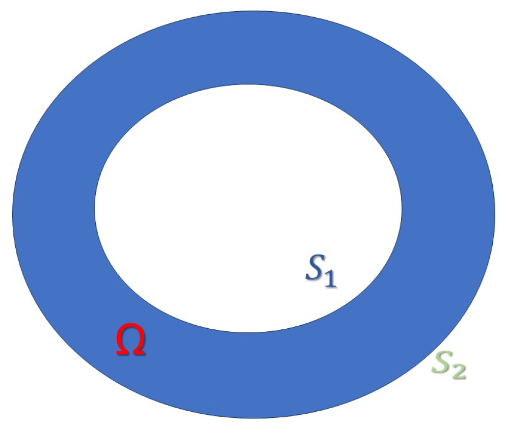
Figure 2.
(a) Exact measurement V (black line) and with error (red line). (b) Exact potential and its approximations and applying regularization and without regularization, corresponding to the Example 1 for (see Table 1). We take and in this case.
Figure 2.
(a) Exact measurement V (black line) and with error (red line). (b) Exact potential and its approximations and applying regularization and without regularization, corresponding to the Example 1 for (see Table 1). We take and in this case.
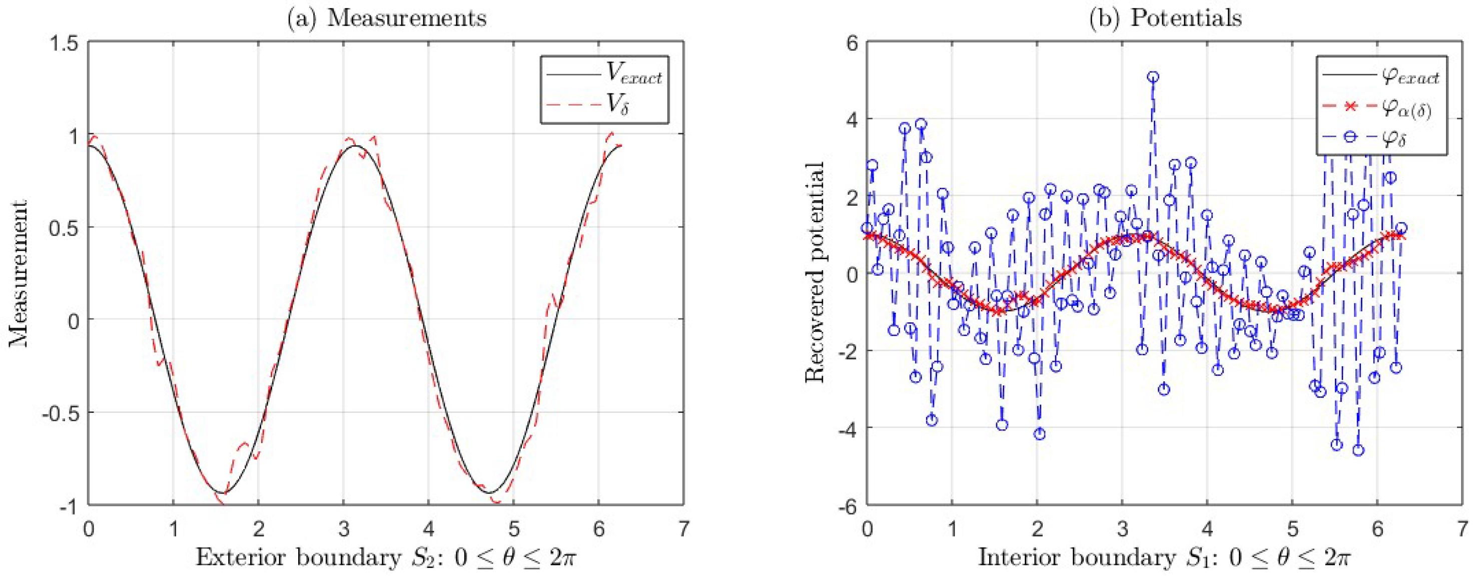
Figure 3.
(a) Exact measurement V (black line) and with error (red line). (b) Exact potential and its approximations and applying regularization and without regularization, corresponding to the Example 2 for (see Table 2). In this case, we take and
Figure 3.
(a) Exact measurement V (black line) and with error (red line). (b) Exact potential and its approximations and applying regularization and without regularization, corresponding to the Example 2 for (see Table 2). In this case, we take and
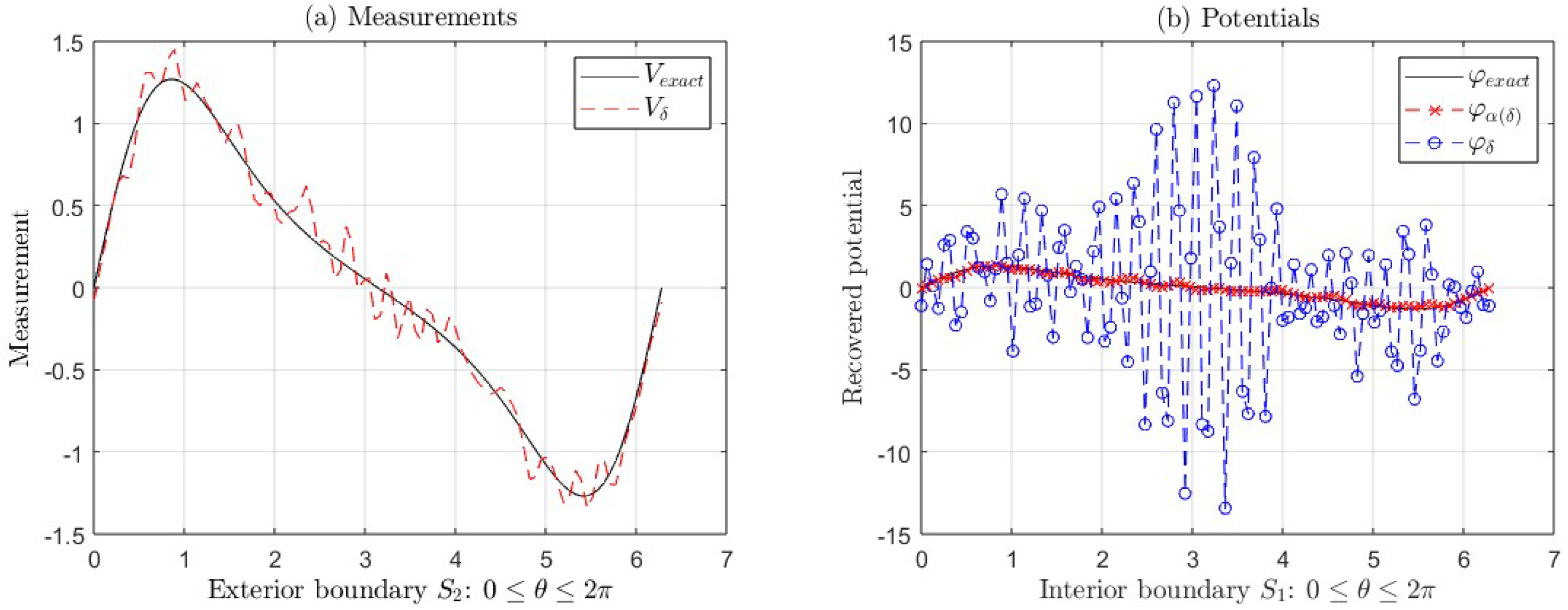
Figure 4.
(a) Exact measurement V (black line) and with error (red line). (b) Exact potential and its approximations and , corresponding to the Example 1 for (see Table 3). In this case, we take and .
Figure 4.
(a) Exact measurement V (black line) and with error (red line). (b) Exact potential and its approximations and , corresponding to the Example 1 for (see Table 3). In this case, we take and .
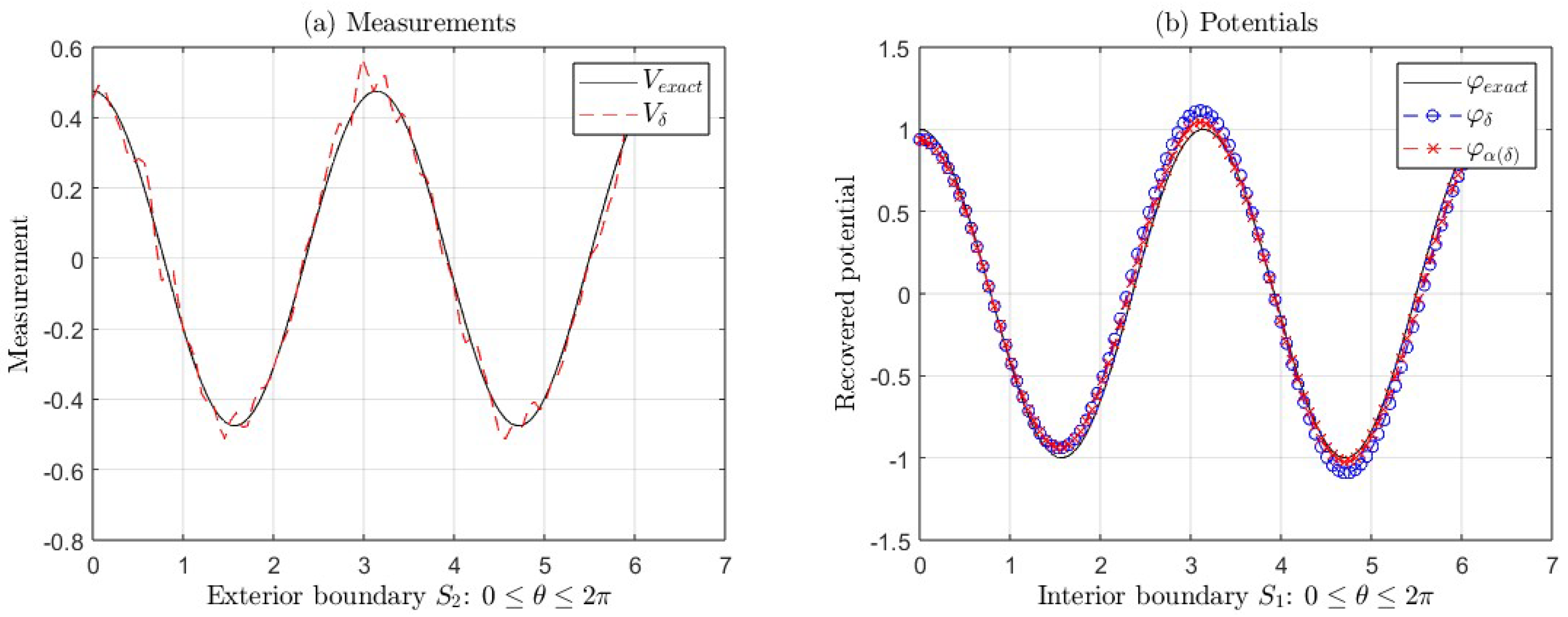
Figure 5.
(a) Exact measurement V (black line) and with error (red line). (b) Exact potential and its approximations and , corresponding to the Example 2 for (see Table 4). In this case, we take and .
Figure 5.
(a) Exact measurement V (black line) and with error (red line). (b) Exact potential and its approximations and , corresponding to the Example 2 for (see Table 4). In this case, we take and .
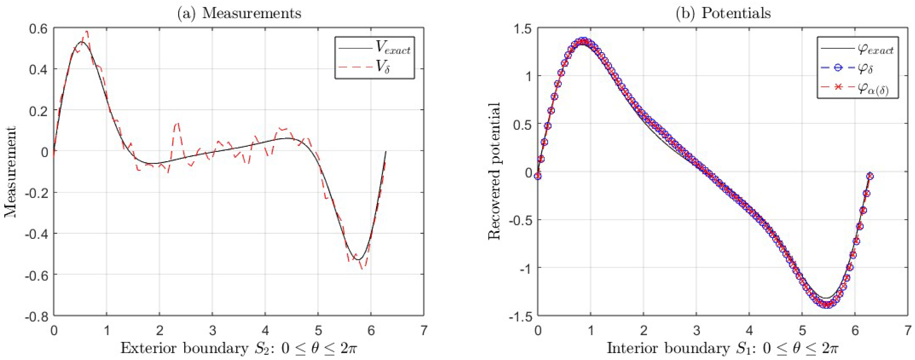
Figure 6.
(a) Exact measurement V (black line) and with error (red line). (b) Exact potential and its approximations and , corresponding to the Example 1 for , and (see Table 5). In this case, we take and .
Figure 6.
(a) Exact measurement V (black line) and with error (red line). (b) Exact potential and its approximations and , corresponding to the Example 1 for , and (see Table 5). In this case, we take and .
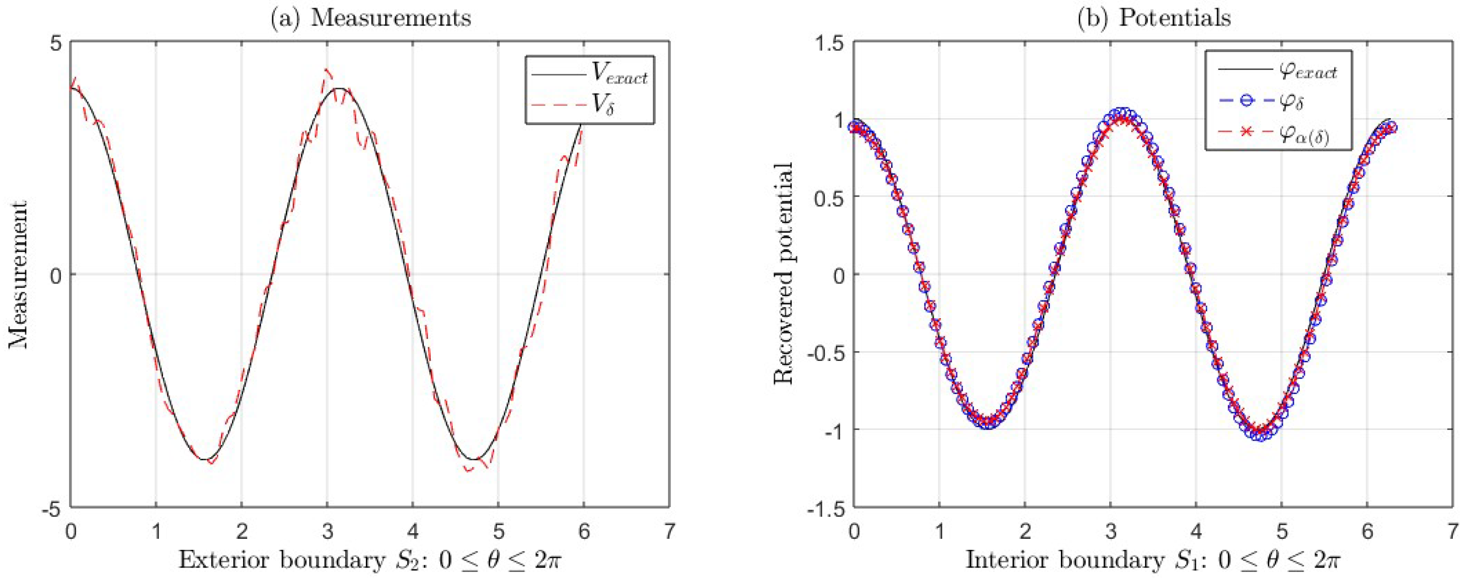
Figure 7.
(a) Exact measurement V (black line) and with error (red line). (b) Exact potential and its approximations and , corresponding to the Example 1 for , and (see Table 5). In this case, we take and .
Figure 7.
(a) Exact measurement V (black line) and with error (red line). (b) Exact potential and its approximations and , corresponding to the Example 1 for , and (see Table 5). In this case, we take and .
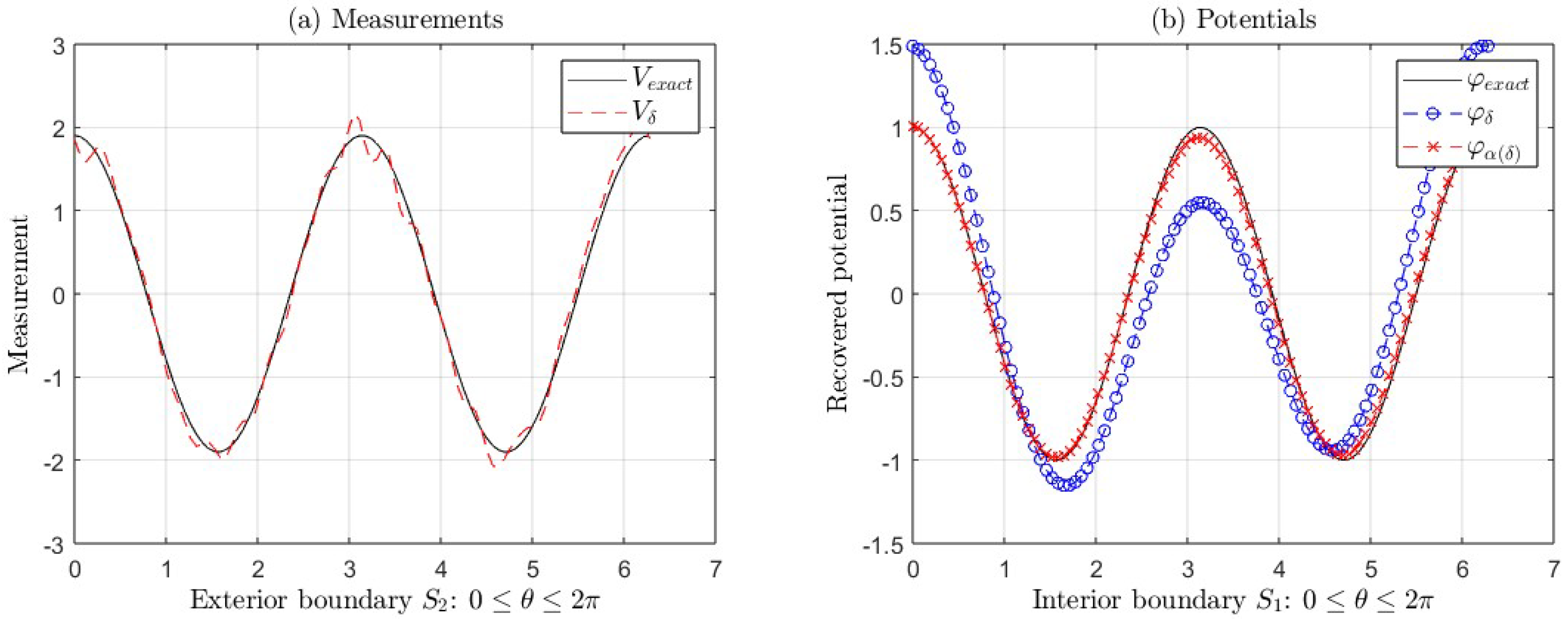
Figure 8.
(a) Exact measurement V (black line) and with error (red line). (b) Exact potential and its approximations and , corresponding to the Example 2 for , and (see Table 6). In this case, we take and .
Figure 8.
(a) Exact measurement V (black line) and with error (red line). (b) Exact potential and its approximations and , corresponding to the Example 2 for , and (see Table 6). In this case, we take and .
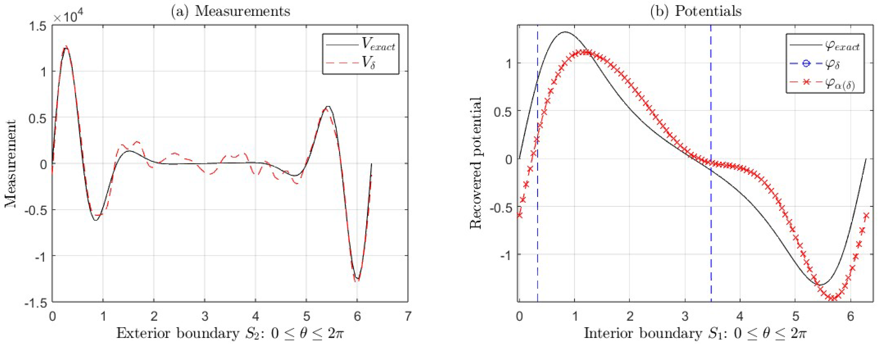
Figure 9.
(a) Exact measurement V (black line) and with error (red line). (b) Exact potential and its approximations and , corresponding to the Example 1 for , and (see Table 7). In this case, we take and .
Figure 9.
(a) Exact measurement V (black line) and with error (red line). (b) Exact potential and its approximations and , corresponding to the Example 1 for , and (see Table 7). In this case, we take and .
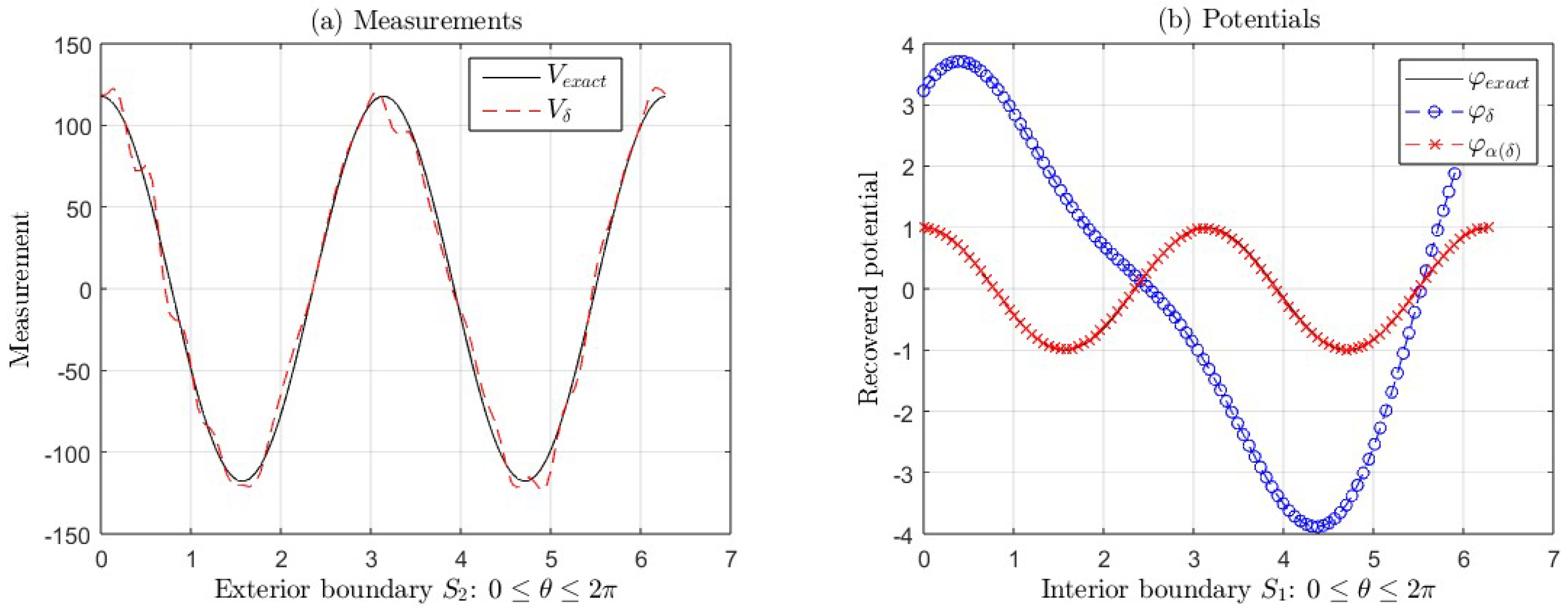
Figure 10.
(a) Exact measurement V (black line) and with error (red line). (b) Exact potential and its approximations and , corresponding to the Example 1 for , and (see Table 8). In this case, we take and .
Figure 10.
(a) Exact measurement V (black line) and with error (red line). (b) Exact potential and its approximations and , corresponding to the Example 1 for , and (see Table 8). In this case, we take and .
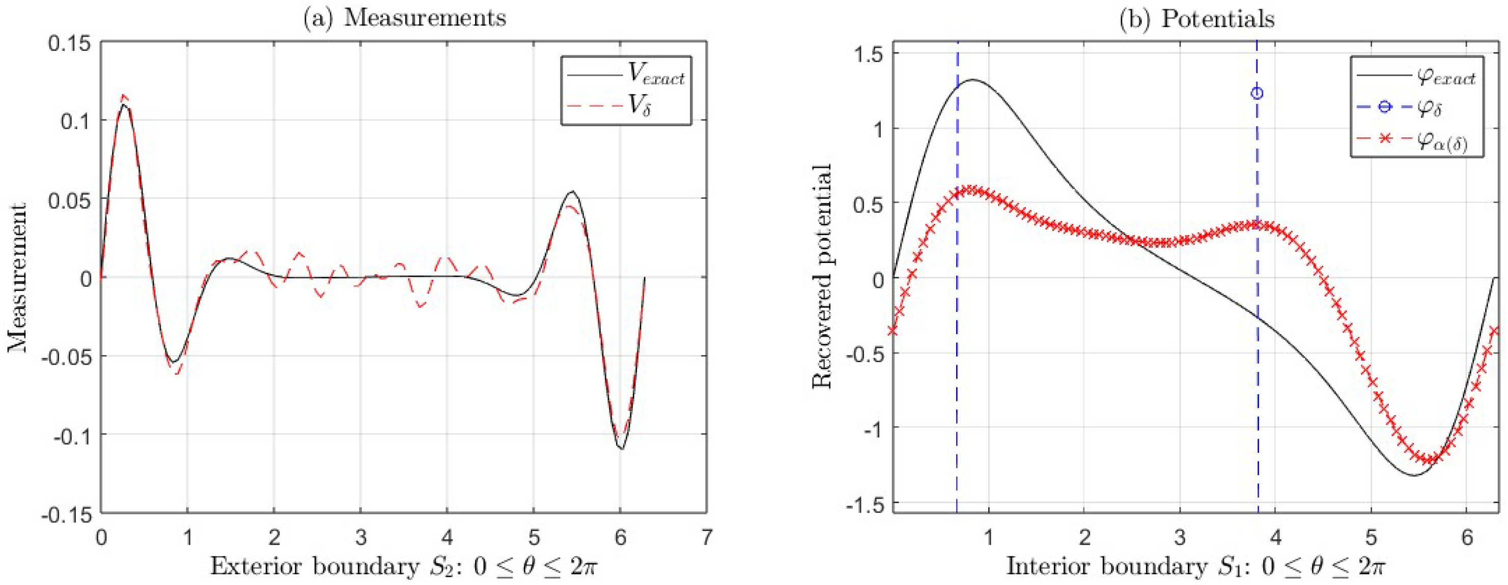
Figure 11.
(a) Exact measurement V (black line) and with error (red line). (b) Exact potential and its approximations and , corresponding to the Example 1 for , and (see Table 9). In this case, we take and .
Figure 11.
(a) Exact measurement V (black line) and with error (red line). (b) Exact potential and its approximations and , corresponding to the Example 1 for , and (see Table 9). In this case, we take and .
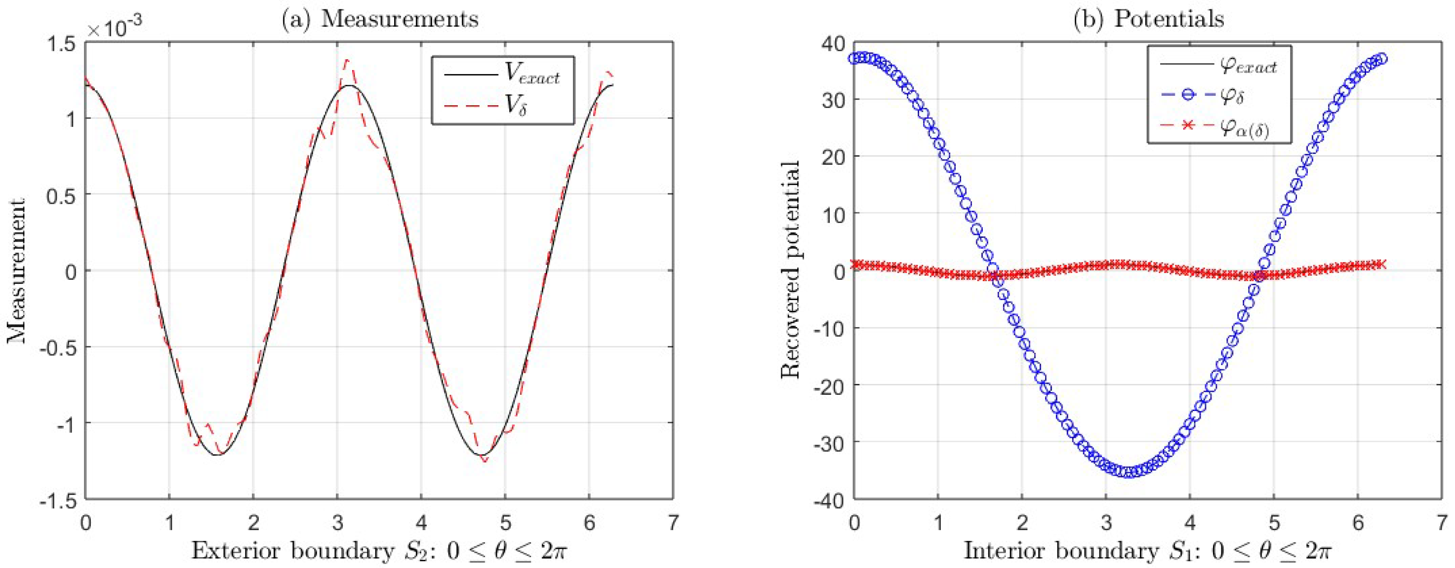
Figure 12.
(a) Exact measurement V (black line) and with error (red line). (b) Exact potential and its approximations and , corresponding to the Example 2 for , and (see Table 10). In this case, we take and .
Figure 12.
(a) Exact measurement V (black line) and with error (red line). (b) Exact potential and its approximations and , corresponding to the Example 2 for , and (see Table 10). In this case, we take and .
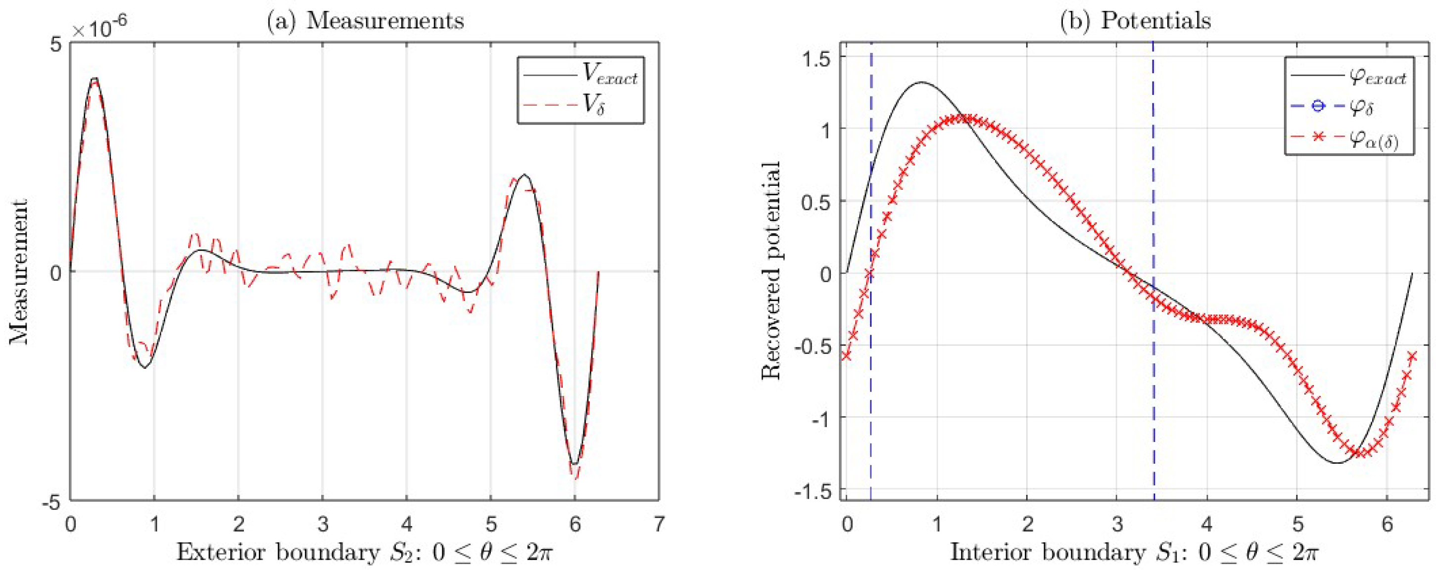
Figure 13.
(a) Exact measurement V (black line) and with error (red line). (b) Exact potential and its approximations and , corresponding to the Example 1 for , and (see Table 11). In this case, we take and .
Figure 13.
(a) Exact measurement V (black line) and with error (red line). (b) Exact potential and its approximations and , corresponding to the Example 1 for , and (see Table 11). In this case, we take and .
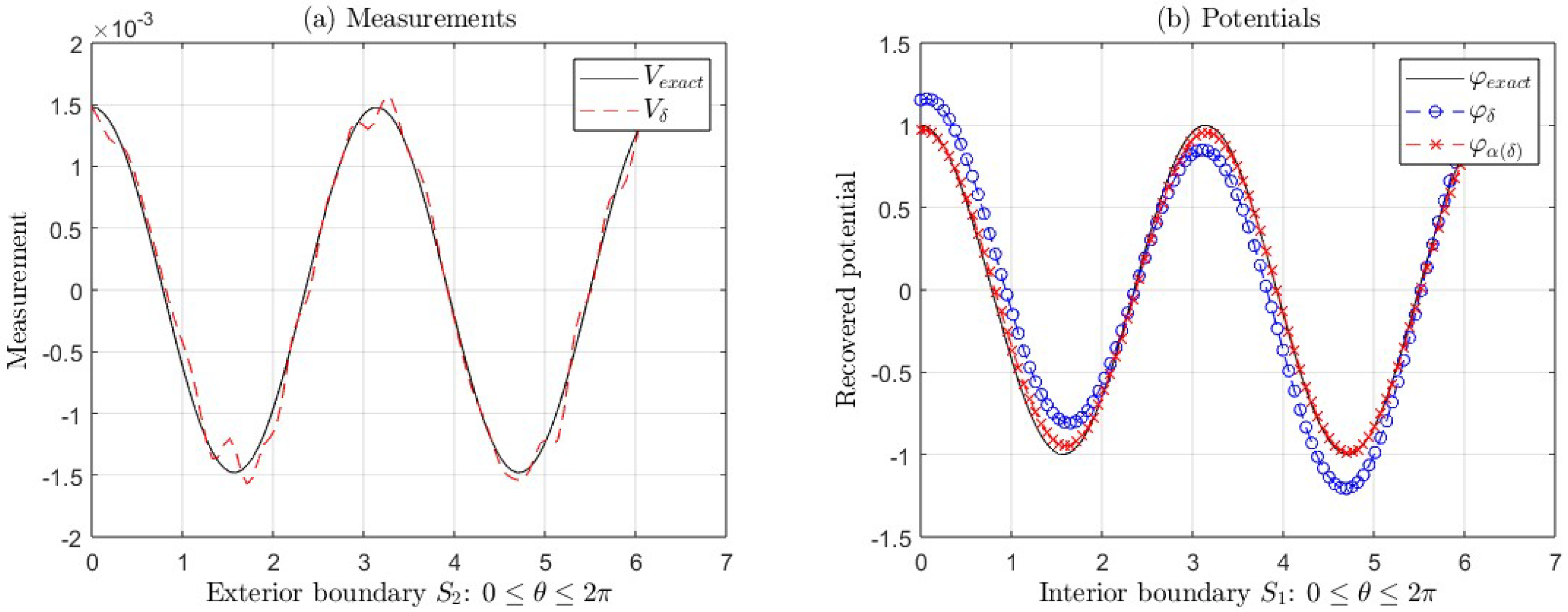
Figure 14.
(a) Exact measurement V (black line) and with error (red line). (b) Exact potential and its approximations and , corresponding to the Example 1 for , and (see Table 11). In this case, we take and .
Figure 14.
(a) Exact measurement V (black line) and with error (red line). (b) Exact potential and its approximations and , corresponding to the Example 1 for , and (see Table 11). In this case, we take and .
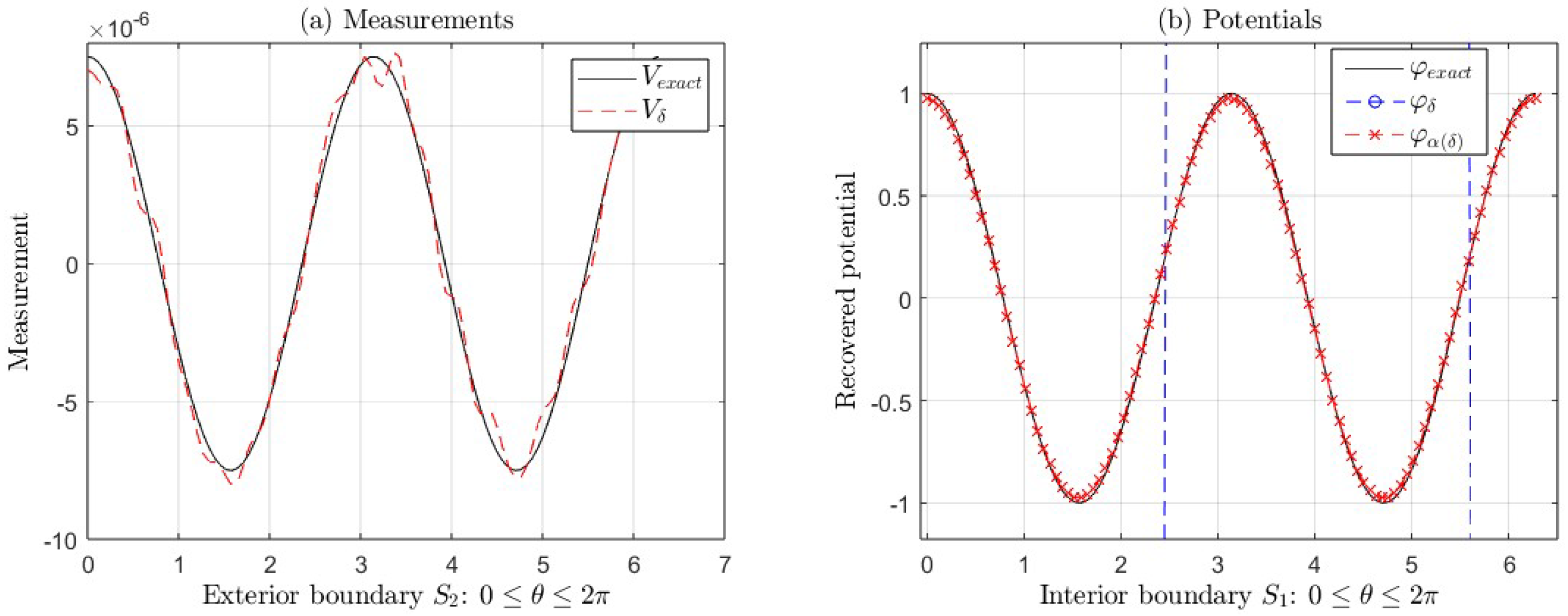
Figure 15.
(a) Exact measurement V (black line) and with error (red line). (b) Exact potential and its approximations and , corresponding to the Example 2 for , and (see Table 12). In this case, we take and .
Figure 15.
(a) Exact measurement V (black line) and with error (red line). (b) Exact potential and its approximations and , corresponding to the Example 2 for , and (see Table 12). In this case, we take and .
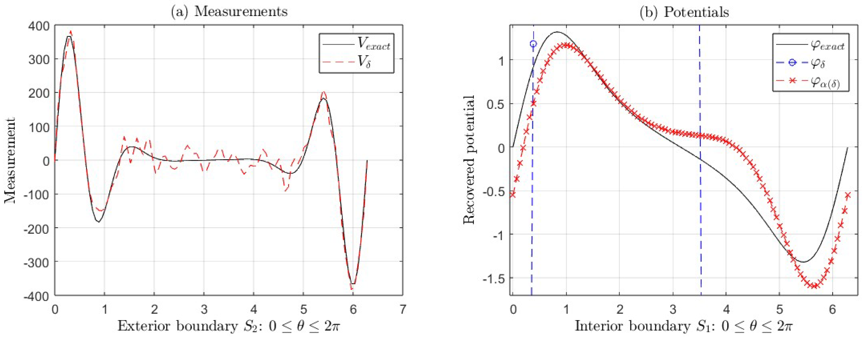
Figure 16.
(a) Exact measurement V (black line) and with error (red line). (b) Exact potential and its approximations and , corresponding to the Example 2 for , and (see Table 12). In this case, we take and .
Figure 16.
(a) Exact measurement V (black line) and with error (red line). (b) Exact potential and its approximations and , corresponding to the Example 2 for , and (see Table 12). In this case, we take and .
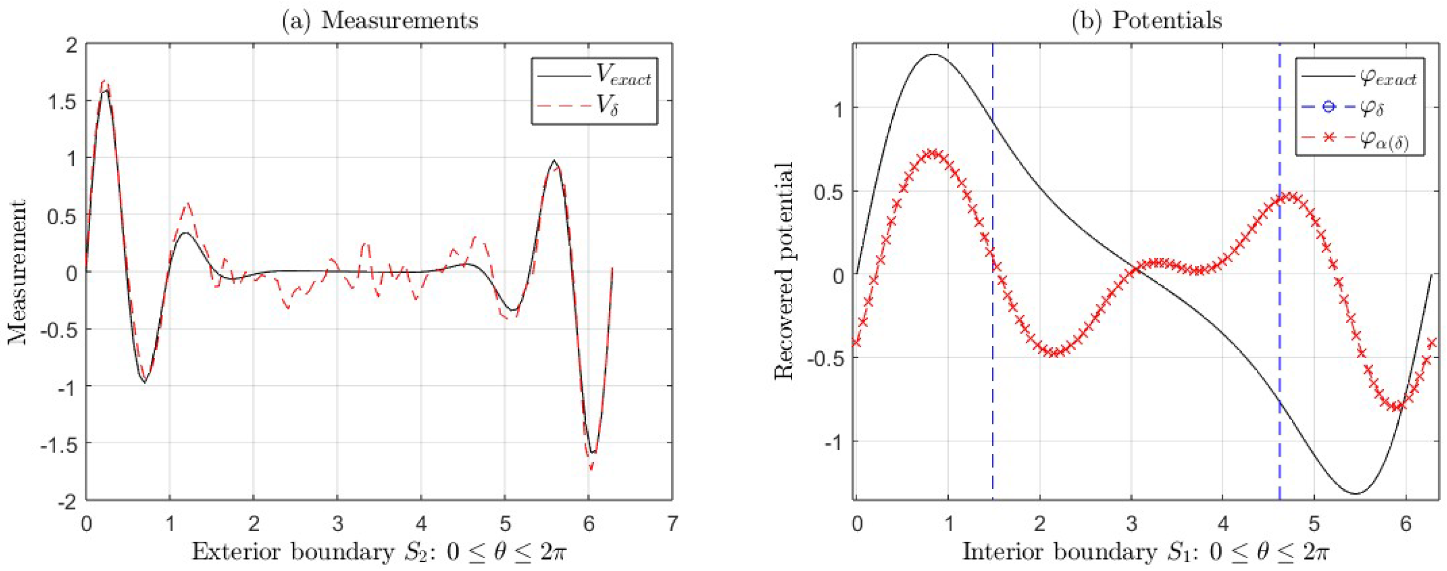

Table 1.
Numerical results applying TRM to solve the IP related to the classical Cauchy problem (2), for , , and different values of and N.
Table 1.
Numerical results applying TRM to solve the IP related to the classical Cauchy problem (2), for , , and different values of and N.
| N | |||||
|---|---|---|---|---|---|
| 0 | 20 | 0 | 0 | 0 | 0 |
| 0.1 | 20 | 0.1 | 0.1069 | 0.1465 | 0.8224 |
| 0.1 | 25 | 0.1 | 0.1034 | 0.1471 | 1.6048 |
| 0.1 | 30 | 0.1 | 0.1126 | 0.1435 | 3.0063 |
| 0.01 | 20 | 0.01 | 0.0102 | 0.0342 | 0.0663 |
| 0.01 | 25 | 0.01 | 0.0112 | 0.0360 | 0.2137 |
| 0.01 | 30 | 0.01 | 0.0114 | 0.0362 | 0.4820 |
| 0.001 | 20 | 0.001 | 9.0770 | 0.0050 | 0.0057 |
| 0.001 | 25 | 0.001 | 8.8517 | 0.0068 | 0.0122 |
| 0.001 | 30 | 0.001 | 9.5479 | 0.0083 | 0.0354 |
Table 2.
Numerical results applying TRM to solve the IP related to the classical Cauchy problem (2), for , and different values of and N.
Table 2.
Numerical results applying TRM to solve the IP related to the classical Cauchy problem (2), for , and different values of and N.
| N | |||||
|---|---|---|---|---|---|
| 0 | 18 | 0 | 0 | 2.5338 | 2.4537 |
| 0.1 | 18 | 0.1 | 0.1161 | 0.1590 | 0.8005 |
| 0.1 | 25 | 0.1 | 0.1125 | 0.1571 | 1.6366 |
| 0.1 | 30 | 0.1 | 0.1340 | 0.1512 | 5.7825 |
| 0.01 | 18 | 0.01 | 0.0117 | 0.0357 | 0.0509 |
| 0.01 | 25 | 0.01 | 0.0105 | 0.0392 | 0.1485 |
| 0.01 | 30 | 0.01 | 0.0112 | 0.0364 | 0.3478 |
| 0.001 | 18 | 0.001 | 8.8274 | 0.0046 | 0.0048 |
| 0.001 | 25 | 0.001 | 9.9199 | 0.0095 | 0.0162 |
| 0.001 | 30 | 0.001 | 0.0011 | 0.0099 | 0.0423 |
Table 3.
Numerical results applying TRM to solve IP related to the fractional Cauchy problem (12), for , , and different values of and N.
Table 3.
Numerical results applying TRM to solve IP related to the fractional Cauchy problem (12), for , , and different values of and N.
| N | m | ||||||
|---|---|---|---|---|---|---|---|
| 0 | 20 | 0 | 0.5 | 1 | 0 | 1.1102 | 0 |
| 0.1 | 20 | 1 | 0.5 | 1 | 0.0970 | 0.0617 | 0.0880 |
| 0.1 | 25 | 1 | 0.5 | 1 | 0.0979 | 0.0719 | 0.0990 |
| 0.1 | 30 | 1 | 0.5 | 1 | 0.1038 | 0.0775 | 0.1217 |
| 0.01 | 20 | 1 | 0.5 | 1 | 0.0093 | 0.0037 | 0.0039 |
| 0.01 | 25 | 1 | 0.5 | 1 | 0.0091 | 0.0070 | 0.0070 |
| 0.01 | 30 | 1 | 0.5 | 1 | 0.0127 | 0.0072 | 0.0073 |
| 0.001 | 20 | 1 | 0.5 | 1 | 9.6950 | 8.9805 | 8.9826 |
| 0.001 | 25 | 1 | 0.5 | 1 | 8.3006 | 3.4557 | 3.4620 |
| 0.001 | 30 | 1 | 0.5 | 1 | 9.8327 | 5.4898 | 5.4925 |
Table 4.
Numerical results applying TRM to solve IP related to the fractional Cauchy problem (12), for , , and different values of and N.
Table 4.
Numerical results applying TRM to solve IP related to the fractional Cauchy problem (12), for , , and different values of and N.
| N | m | ||||||
|---|---|---|---|---|---|---|---|
| 0 | 18 | 0 | 0.5 | 1 | 0 | 2.4537 | 2.4537 |
| 0.1 | 18 | 1 | 0.5 | 1 | 0.1292 | 0.1196 | 0.1212 |
| 0.1 | 25 | 1 | 0.5 | 1 | 0.1732 | 0.1238 | 0.1296 |
| 0.1 | 30 | 1 | 0.5 | 1 | 0.1921 | 0.0624 | 0.0672 |
| 0.01 | 18 | 1 | 0.5 | 1 | 0.0147 | 0.0126 | 0.0129 |
| 0.01 | 25 | 1 | 0.5 | 1 | 0.0166 | 0.0124 | 0.0129 |
| 0.01 | 30 | 1 | 0.5 | 1 | 0.0177 | 0.0069 | 0.0071 |
| 0.001 | 18 | 1 | 0.5 | 1 | 0.0012 | 8.6623 | 9.1811 |
| 0.001 | 25 | 1 | 0.5 | 1 | 0.0017 | 8.6801 | 9.1904 |
| 0.001 | 25 | 1 | 0.5 | 1 | 0.0018 | 7.3211 | 7.7961 |
Table 5.
Numerical results applying TRM to solve IP related to the fractional Cauchy problem (12) for and different values of and m, where , .
Table 5.
Numerical results applying TRM to solve IP related to the fractional Cauchy problem (12) for and different values of and m, where , .
| N | m | |||||
|---|---|---|---|---|---|---|
| 20 | 1 | 1.5 | 2 | 0.1027 | 0.0360 | 0.0392 |
| 25 | 8 | 1.5 | 2 | 0.1017 | 0.0518 | 0.0819 |
| 30 | 5 | 1.5 | 2 | 0.1136 | 0.0597 | 0.0718 |
| 20 | 2 | 2.5 | 3 | 0.0936 | 0.0508 | 0.4857 |
| 20 | 1 | 3.5 | 4 | 0.0969 | 0.0474 | 0.3523 |
| 20 | 1 | 4.5 | 5 | 0.0915 | 0.0421 | 1.5924 |
| 20 | 1 | 5.5 | 6 | 0.1112 | 0.0248 | 1.2606 |
| 20 | 1 | 6.5 | 7 | 0.1078 | 0.0366 | 5.8758 |
| 20 | 1 | 7.5 | 8 | 0.1045 | 0.0351 | 2.2946 |
| 20 | 1 | 8.5 | 9 | 0.0916 | 0.0197 | 16.6149 |
| 20 | 1 | 9.5 | 10 | 0.0996 | 0.0274 | 21.0258 |
| 20 | 1 | 10.5 | 11 | 0.0939 | 0.0176 | 46.6720 |
| 20 | 1 | 11.5 | 12 | 0.0861 | 0.0407 | 33.8060 |
Table 6.
Numerical results applying TRM to solve IP related to the fractional Cauchy problem (12) for and different values of and m, where , .
Table 6.
Numerical results applying TRM to solve IP related to the fractional Cauchy problem (12) for and different values of and m, where , .
| N | m | |||||
|---|---|---|---|---|---|---|
| 18 | 1 | 1.5 | 2 | 0.1279 | 0.0342 | 0.0411 |
| 25 | 1 | 1.5 | 2 | 0.1780 | 0.0258 | 0.0264 |
| 30 | 1 | 1.5 | 2 | 0.1732 | 0.0439 | 0.0509 |
| 18 | 9 | 2.5 | 3 | 0.1629 | 0.1437 | 0.1504 |
| 18 | 4 | 3.5 | 4 | 0.1461 | 0.0931 | 0.3543 |
| 18 | 1.4 | 4.5 | 5 | 0.1466 | 0.1385 | 7.4132 |
| 18 | 1 | 5.5 | 6 | 0.1757 | 0.3306 | 9.1616 |
| 18 | 1 | 6.5 | 7 | 0.1512 | 0.3654 | 478.6290 |
| 18 | 4.2 | 7.5 | 8 | 0.1643 | 0.3822 | 310.6255 |
| 18 | 3 | 8.5 | 9 | 0.1732 | 0.8982 | 633.1135 |
| 18 | 2 | 9.5 | 10 | 0.2062 | 0.9546 | 4.0208 |
| 18 | 2 | 10.5 | 11 | 0.1712 | 0.8948 | 1.9672 |
| 18 | 8 | 11.5 | 12 | 0.1636 | 0.9326 | 2.2607 |
Table 7.
Numerical results applying TRM to solve the IP related to the fractional Cauchy problem (12) for and different values of and m, where , .
Table 7.
Numerical results applying TRM to solve the IP related to the fractional Cauchy problem (12) for and different values of and m, where , .
| N | m | |||||
|---|---|---|---|---|---|---|
| 20 | 1 | 0.1 | 1 | 0.1093 | 0.0565 | 0.0765 |
| 20 | 1 | 0.0001 | 1 | 0.1032 | 0.0699 | 0.0705 |
| 20 | 1 | 0.0000001 | 1 | 0.1040 | 0.0394 | 0.0394 |
| 20 | 1 | 0.9 | 1 | 0.0922 | 0.0809 | 0.0817 |
| 20 | 1 | 0.9999 | 1 | 0.0988 | 0.0581 | 0.0583 |
| 20 | 1 | 0.9999999 | 1 | 0.0967 | 0.0921 | 0.1277 |
| 20 | 1 | 1.1 | 2 | 0.1081 | 0.0563 | 0.0647 |
| 20 | 5 | 1.0001 | 2 | 0.0931 | 0.0791 | 0.0984 |
| 20 | 1 | 1.0000001 | 2 | 0.0979 | 0.0901 | 0.0953 |
| 20 | 1 | 1.9 | 2 | 0.0980 | 0.0726 | 0.0746 |
| 20 | 1 | 1.9999 | 2 | 0.0971 | 0.0449 | 0.0488 |
| 20 | 1 | 1.9999999 | 2 | 0.1033 | 0.0997 | 0.1105 |
| 20 | 1 | 2.1 | 3 | 0.0998 | 0.0392 | 0.2108 |
| 20 | 1 | 2.0001 | 3 | 0.0905 | 0.0479 | 0.3250 |
| 20 | 1 | 2.0000001 | 3 | 0.0894 | 0.0264 | 0.1021 |
| 20 | 1 | 2.9 | 3 | 0.1110 | 0.0860 | 0.1731 |
| 20 | 1 | 2.9999 | 3 | 0.0999 | 0.0804 | 0.4756 |
| 20 | 1 | 2.9999999 | 3 | 0.1027 | 0.0672 | 0.3546 |
| 20 | 1 | 3.1 | 4 | 0.1061 | 0.0328 | 0.1583 |
| 20 | 1 | 3.9 | 4 | 0.1061 | 0.0738 | 0.5624 |
| 20 | 1 | 4.1 | 5 | 0.0863 | 0.0421 | 1.8856 |
| 20 | 1 | 4.9 | 5 | 0.1030 | 0.0401 | 0.2528 |
| 20 | 1 | 5.1 | 6 | 0.0751 | 0.0368 | 1.5197 |
| 20 | 1 | 5.9 | 6 | 0.0957 | 0.0438 | 1.0323 |
| 20 | 1 | 6.1 | 7 | 0.0917 | 0.0267 | 5.3155 |
| 20 | 1 | 6.9 | 7 | 0.1020 | 0.0600 | 5.5627 |
| 20 | 1 | 7.1 | 8 | 0.0935 | 0.0199 | 3.3483 |
| 20 | 1 | 7.0000001 | 8 | 0.0827 | 0.0206 | 1.7258 |
| 20 | 1 | 7.9 | 8 | 0.0870 | 0.0212 | 4.5019 |
| 20 | 1 | 7.9999999 | 8 | 0.0986 | 0.0454 | 4.2454 |
| 20 | 1 | 8.1 | 9 | 0.1155 | 0.0276 | 14.3075 |
| 20 | 1 | 8.9 | 9 | 0.0953 | 0.0342 | 34.0155 |
| 20 | 1 | 9.1 | 10 | 0.1013 | 0.0508 | 20.6047 |
| 20 | 1 | 9.9 | 10 | 0.0972 | 0.0095 | 24.1306 |
| 20 | 1 | 10.1 | 11 | 0.0941 | 0.0271 | 35.0730 |
| 20 | 1 | 10.9 | 11 | 0.0956 | 0.0090 | 90.0697 |
| 20 | 1 | 11.1 | 12 | 0.0951 | 0.0226 | 65.9229 |
| 20 | 1 | 11.9 | 12 | 0.0967 | 0.0475 | 101.7022 |
Table 8.
Numerical results applying TRM to solve IP related to the fractional Cauchy problem (12) for and different values of and m, where ,
Table 8.
Numerical results applying TRM to solve IP related to the fractional Cauchy problem (12) for and different values of and m, where ,
| N | m | |||||
|---|---|---|---|---|---|---|
| 30 | 1 | 0.1 | 1 | 0.1429 | 0.0210 | 0.0230 |
| 30 | 1 | 0.0001 | 1 | 0.1849 | 0.0396 | 0.0401 |
| 30 | 1 | 0.0000001 | 1 | 0.1762 | 0.0314 | 0.0314 |
| 30 | 1 | 0.9 | 1 | 0.1674 | 0.0448 | 0.0452 |
| 30 | 1 | 0.9999 | 1 | 0.1299 | 0.0544 | 0.0575 |
| 30 | 1 | 0.9999999 | 1 | 0.1748 | 0.0271 | 0.0272 |
| 30 | 1 | 1.1 | 2 | 0.1613 | 0.0454 | 0.0454 |
| 30 | 1 | 1.0001 | 2 | 0.1829 | 0.0492 | 0.0493 |
| 30 | 1 | 1.0000001 | 2 | 0.1842 | 0.0584 | 0.0585 |
| 30 | 1 | 1.9 | 2 | 0.1739 | 0.0353 | 0.0431 |
| 30 | 1 | 1.9999 | 2 | 0.1870 | 0.0380 | 0.0413 |
| 30 | 1 | 1.9999999 | 2 | 0.1690 | 0.0609 | 0.0674 |
| 30 | 1 | 2.1 | 3 | 0.2071 | 0.0760 | 0.1016 |
| 30 | 1 | 2.0001 | 3 | 0.2114 | 0.1688 | 0.1689 |
| 30 | 2.0000001 | 3 | 0.1877 | 0.1176 | 0.1176 | |
| 30 | 3 | 2.9 | 3 | 0.2256 | 0.1156 | 0.2868 |
| 30 | 1 | 2.9999 | 3 | 0.1676 | 0.0761 | 0.4059 |
| 30 | 5 | 2.9999999 | 3 | 0.2155 | 0.1581 | 0.1751 |
| 30 | 5 | 3.1 | 4 | 0.2057 | 0.1258 | 0.1717 |
| 30 | 1 | 3.9 | 4 | 0.2001 | 0.0881 | 0.3453 |
| 30 | 5 | 4.1 | 5 | 0.2545 | 0.3090 | 16.5294 |
| 30 | 1 | 4.9 | 5 | 0.2011 | 0.2408 | 6.8619 |
| 30 | 4 | 5.1 | 6 | 0.1983 | 0.4226 | 12.4482 |
| 30 | 5 | 5.9 | 6 | 0.2049 | 0.3878 | 7.9340 |
| 30 | 7 | 6.1 | 7 | 0.2124 | 0.4678 | 243.7232 |
| 30 | 6 | 6.9 | 7 | 0.2553 | 0.5497 | 363.0725 |
| 30 | 4 | 7.1 | 8 | 0.2463 | 0.4505 | 123.0513 |
| 30 | 5 | 7.0001 | 8 | 0.2452 | 0.2910 | 240.1527 |
| 30 | 2 | 7.0000001 | 8 | 0.2335 | 0.1839 | 119.2328 |
| 30 | 2 | 7.9 | 8 | 0.2184 | 0.1710 | 402.7594 |
| 30 | 1.3 | 7.9999 | 8 | 0.2308 | 0.3440 | 181.8997 |
| 30 | 2 | 7.9999999 | 8 | 0.1833 | 0.5806 | 164.4764 |
| 30 | 3 | 8.1 | 9 | 0.2548 | 0.8971 | 3.4981 |
| 30 | 2 | 8.9 | 9 | 0.2054 | 0.9059 | 2.8978 |
| 30 | 2 | 9.1 | 10 | 0.2260 | 0.8857 | 6.8133 |
| 30 | 7 | 9.9 | 10 | 0.2241 | 0.8896 | 6.2431 |
| 30 | 4 | 10.1 | 11 | 0.2233 | 0.9011 | 2.5172 |
| 30 | 2 | 10.9 | 11 | 0.2069 | 0.8934 | 1.9773 |
| 30 | 5 | 11.1 | 12 | 0.2479 | 0.9212 | 1.1346 |
| 30 | 5 | 11.9 | 12 | 0.2372 | 0.8996 | 3.4904 |
Table 9.
Numerical results applying TRM to solve the IP related to the fractional Cauchy problem (12) for and different values of and m, where , .
Table 9.
Numerical results applying TRM to solve the IP related to the fractional Cauchy problem (12) for and different values of and m, where , .
| N | m | |||||
|---|---|---|---|---|---|---|
| 20 | 1 | 0.5 | 2 | 0.1037 | 0.0369 | 0.0371 |
| 25 | 1 | 0.5 | 2 | 0.1043 | 0.0846 | 0.0850 |
| 30 | 1 | 0.5 | 2 | 0.1123 | 0.0947 | 0.0952 |
| 20 | 1 | 0.1 | 3 | 0.0953 | 0.0558 | 0.3293 |
| 20 | 1 | 0.8 | 3 | 0.0928 | 0.0397 | 0.1176 |
| 20 | 1 | 1.6 | 4 | 0.1031 | 0.0692 | 0.3781 |
| 20 | 1 | 2.9 | 4 | 0.0988 | 0.0550 | 0.2616 |
| 20 | 1 | 0.5 | 5 | 0.1063 | 0.0493 | 2.3272 |
| 20 | 1 | 3.5 | 5 | 0.1002 | 0.0479 | 0.6521 |
| 20 | 1 | 0.5 | 6 | 0.0824 | 0.0664 | 1.0640 |
| 20 | 1 | 3.4 | 6 | 0.1156 | 0.0541 | 1.0860 |
| 20 | 1 | 0.5 | 7 | 0.1093 | 0.0251 | 11.3550 |
| 20 | 1 | 4.2 | 7 | 0.0871 | 0.0203 | 4.0183 |
| 20 | 1 | 0.5 | 8 | 0.0915 | 0.0280 | 3.7583 |
| 20 | 1 | 3.7 | 8 | 0.1097 | 0.0212 | 4.3335 |
| 20 | 1 | 0.5 | 9 | 0.0969 | 0.0195 | 21.9486 |
| 20 | 1 | 5.2 | 9 | 0.0841 | 0.0345 | 9.1221 |
| 20 | 1 | 0.5 | 10 | 0.1022 | 0.0290 | 22.9009 |
| 20 | 1 | 7.6 | 10 | 0.1073 | 0.0181 | 7.2447 |
| 20 | 1 | 0.5 | 11 | 0.0936 | 0.0300 | 122.7548 |
| 20 | 1 | 6.6 | 11 | 0.0886 | 0.0121 | 91.7074 |
| 20 | 1 | 0.5 | 12 | 0.0926 | 0.0149 | 30.3739 |
| 20 | 1 | 6.3 | 12 | 0.1007 | 0.0329 | 36.2964 |
Table 10.
Numerical results applying TRM to solve IP related to the fractional Cauchy problem (12) for , and different values of m, where , .
Table 10.
Numerical results applying TRM to solve IP related to the fractional Cauchy problem (12) for , and different values of m, where , .
| N | m | |||||
|---|---|---|---|---|---|---|
| 20 | 1 | 0.5 | 2 | 0.1422 | 0.0274 | 0.0284 |
| 25 | 1 | 0.5 | 2 | 0.1537 | 0.0496 | 0.0551 |
| 30 | 1 | 0.5 | 2 | 0.1524 | 0.0585 | 0.0627 |
| 30 | 9 | 0.5 | 3 | 0.1619 | 0.1437 | 0.1438 |
| 30 | 5 | 0.5 | 4 | 0.1960 | 0.1656 | 0.2199 |
| 30 | 7 | 0.5 | 5 | 0.2014 | 0.1376 | 13.9836 |
| 30 | 4 | 0.5 | 6 | 0.2265 | 0.2261 | 8.6601 |
| 30 | 5 | 0.5 | 7 | 0.2419 | 0.2709 | 209.3490 |
| 30 | 5 | 0.5 | 8 | 0.2131 | 0.4002 | 205.2009 |
| 30 | 3 | 0.5 | 9 | 0.2154 | 0.8873 | 2.6220 |
| 30 | 1.4 | 0.5 | 10 | 0.2010 | 0.8863 | 4.1567 |
| 30 | 6 | 0.5 | 11 | 0.2148 | 0.9054 | 1.3299 |
| 30 | 3 | 0.5 | 12 | 0.2021 | 0.8935 | 1.6833 |
Table 11.
Numerical results applying TRM to solve the IP related to the fractional Cauchy problem (12) for and different values of and m, where , .
Table 11.
Numerical results applying TRM to solve the IP related to the fractional Cauchy problem (12) for and different values of and m, where , .
| N | m | |||||
|---|---|---|---|---|---|---|
| 20 | 1 | 0.1 | 2 | 0.0981 | 0.0294 | 0.0312 |
| 20 | 1 | 0.0001 | 2 | 0.0880 | 0.0665 | 0.0702 |
| 20 | 1 | 0.0000001 | 2 | 0.0877 | 0.0420 | 0.0436 |
| 20 | 1 | 0.9 | 2 | 0.0825 | 0.0252 | 0.0301 |
| 20 | 1 | 0.9999 | 2 | 0.0896 | 0.0355 | 0.0383 |
| 20 | 1 | 0.9999999 | 2 | 0.0988 | 0.0497 | 0.0524 |
| 20 | 1 | 0.1 | 3 | 0.0984 | 0.0736 | 0.4041 |
| 20 | 1 | 0.0001 | 3 | 0.0988 | 0.0556 | 0.2586 |
| 20 | 1 | 0.0000001 | 3 | 0.1063 | 0.0633 | 0.5828 |
| 20 | 1 | 0.9 | 3 | 0.0824 | 0.0632 | 0.2671 |
| 20 | 1 | 0.9999 | 3 | 0.0940 | 0.0747 | 0.4997 |
| 20 | 5 | 0.9999999 | 3 | 0.0843 | 0.0582 | 0.2323 |
| 20 | 1 | 2.1 | 4 | 0.1133 | 0.0813 | 0.4297 |
| 20 | 1 | 2.9 | 4 | 0.1097 | 0.0494 | 0.2746 |
| 20 | 1 | 3.1 | 5 | 0.0841 | 0.0521 | 0.5721 |
| 20 | 1 | 3.9 | 5 | 0.0923 | 0.0284 | 0.9725 |
| 20 | 1 | 4.1 | 6 | 0.0982 | 0.0441 | 1.3912 |
| 20 | 1 | 4.9 | 6 | 0.1192 | 0.0261 | 0.2905 |
| 20 | 1 | 5.1 | 7 | 0.1027 | 0.0331 | 12.2005 |
| 20 | 1 | 5.9 | 7 | 0.0926 | 0.0324 | 2.2300 |
| 20 | 1 | 5.1 | 8 | 0.0928 | 0.0306 | 2.3248 |
| 20 | 1 | 5.0001 | 8 | 0.0936 | 0.0312 | 5.2064 |
| 20 | 1 | 5.0000001 | 8 | 0.1020 | 0.0174 | 1.3253 |
| 20 | 1 | 5.9 | 8 | 0.0967 | 0.0113 | 3.4116 |
| 20 | 1 | 5.9999 | 8 | 0.0946 | 0.0260 | 7.0605 |
| 20 | 1 | 5.9999999 | 8 | 0.0907 | 0.0275 | 1.9174 |
| 20 | 1 | 7.1 | 9 | 0.0849 | 0.0118 | 9.9754 |
| 20 | 1 | 7.9 | 9 | 0.0916 | 0.0224 | 16.5564 |
| 20 | 1 | 3.1 | 10 | 0.0930 | 0.0114 | 20.7949 |
| 20 | 1 | 3.9 | 10 | 0.1054 | 0.0197 | 31.4437 |
| 20 | 1 | 6.1 | 11 | 0.0978 | 0.0207 | 79.4649 |
| 20 | 1 | 6.9 | 11 | 0.1048 | 0.0109 | 59.7459 |
| 20 | 1 | 4.1 | 12 | 0.1035 | 0.0133 | 108.9786 |
| 20 | 1 | 4.9 | 12 | 0.0978 | 0.0278 | 131.9629 |
Table 12.
Numerical results applying TRM to solve the IP related to the fractional Cauchy problem (12) for and different values of and m, where , .
Table 12.
Numerical results applying TRM to solve the IP related to the fractional Cauchy problem (12) for and different values of and m, where , .
| N | m | |||||
|---|---|---|---|---|---|---|
| 30 | 1 | 0.1 | 2 | 0.1918 | 0.0633 | 0.0669 |
| 30 | 1 | 0.0001 | 2 | 0.1747 | 0.0510 | 0.0551 |
| 30 | 1 | 0.0000001 | 2 | 0.1932 | 0.0408 | 0.0466 |
| 30 | 1 | 0.9 | 2 | 0.1678 | 0.0267 | 0.0338 |
| 30 | 1 | 0.9999 | 2 | 0.1879 | 0.0538 | 0.0996 |
| 30 | 1 | 0.9999999 | 2 | 0.1757 | 0.0330 | 0.0352 |
| 30 | 7 | 0.1 | 3 | 0.2035 | 0.1269 | 0.3288 |
| 30 | 3 | 0.0001 | 3 | 0.1945 | 0.0741 | 0.2384 |
| 30 | 6 | 0.0000001 | 3 | 0.1863 | 0.2035 | 0.2102 |
| 30 | 7 | 0.9 | 3 | 0.2208 | 0.1301 | 0.2493 |
| 30 | 2 | 0.9999 | 3 | 0.2057 | 0.0770 | 0.2885 |
| 30 | 5 | 0.9999999 | 3 | 0.2013 | 0.1809 | 0.2036 |
| 30 | 1 | 2.1 | 4 | 0.2001 | 0.1393 | 0.1397 |
| 30 | 3 | 2.9 | 4 | 0.1984 | 0.1061 | 0.2367 |
| 30 | 2 | 3.1 | 5 | 0.2106 | 0.2788 | 14.4371 |
| 30 | 6 | 3.9 | 5 | 0.1827 | 0.2914 | 6.9833 |
| 30 | 1 | 4.1 | 6 | 0.2299 | 0.3008 | 4.2311 |
| 30 | 5 | 4.9 | 6 | 0.1770 | 0.2723 | 3.9078 |
| 30 | 3 | 5.1 | 7 | 0.2095 | 0.1755 | 297.5818 |
| 30 | 5 | 5.9 | 7 | 0.1969 | 0.3580 | 51.0331 |
| 30 | 2 | 5.1 | 8 | 0.2424 | 0.2924 | 216.7317 |
| 30 | 3 | 5.0001 | 8 | 0.2004 | 0.3714 | 452.3457 |
| 30 | 1.4 | 5.0000001 | 8 | 0.1747 | 0.3650 | 239.9826 |
| 30 | 2 | 5.9 | 8 | 0.2001 | 0.3549 | 263.7365 |
| 30 | 1.3 | 5.9999 | 8 | 0.1829 | 0.3781 | 78.5332 |
| 30 | 5 | 5.9999999 | 8 | 0.2137 | 0.2490 | 311.6103 |
| 30 | 1.5 | 7.1 | 9 | 0.2263 | 0.8972 | 4.5033 |
| 30 | 1 | 7.9 | 9 | 0.2228 | 0.8943 | 4.3085 |
| 30 | 1 | 3.1 | 10 | 0.2658 | 0.8914 | 7.9703 |
| 30 | 8 | 3.9 | 10 | 0.2642 | 0.8948 | 5.5828 |
| 30 | 1 | 6.1 | 11 | 0.2378 | 0.9312 | 2.8572 |
| 30 | 5 | 6.9 | 11 | 0.2089 | 0.8950 | 5.1113 |
| 30 | 2 | 4.1 | 12 | 0.2311 | 0.8945 | 7.0888 |
| 30 | 4 | 4.9 | 12 | 0.1994 | 0.9057 | 7.9818 |
Table 13.
Numerical results applying TRM to solve IP related to the fractional Cauchy problem (12) for and different values of and m, where , .
Table 13.
Numerical results applying TRM to solve IP related to the fractional Cauchy problem (12) for and different values of and m, where , .
| N | m | |||||
|---|---|---|---|---|---|---|
| 20 | 1 | 1.001 | 1 | 0.0949 | 0.0430 | 0.0432 |
| 20 | 1 | 1.5 | 1 | 0.0860 | 0.0825 | 0.0965 |
| 20 | 1 | 2.0001 | 2 | 0.0911 | 0.0574 | 0.0581 |
| 20 | 1 | 3.1 | 2 | 0.0809 | 0.0783 | 0.0863 |
| 20 | 1 | 3.01 | 3 | 0.0894 | 0.0278 | 0.1076 |
| 20 | 1 | 4.5 | 3 | 0.1048 | 0.0639 | 0.2370 |
| 20 | 1 | 4.1 | 4 | 0.0942 | 0.0294 | 0.1592 |
| 20 | 1 | 7.1 | 4 | 0.1051 | 0.0495 | 0.2588 |
| 20 | 1 | 5.0001 | 5 | 0.0792 | 0.0298 | 1.3533 |
| 20 | 1 | 6.1 | 5 | 0.0946 | 0.0165 | 0.4475 |
| 20 | 1 | 6.1 | 6 | 0.0907 | 0.0277 | 0.9987 |
| 20 | 1 | 7.5 | 6 | 0.0867 | 0.0276 | 0.6014 |
| 20 | 1 | 7.1 | 7 | 0.0932 | 0.0109 | 3.5379 |
| 20 | 1 | 8.6 | 7 | 0.1024 | 0.0131 | 3.1745 |
| 20 | 1 | 8.001 | 8 | 0.1135 | 0.0277 | 2.2757 |
| 20 | 1 | 9.4 | 8 | 0.0877 | 0.0180 | 3.6123 |
| 20 | 1 | 9.0001 | 9 | 0.0935 | 0.0163 | 22.9725 |
| 20 | 1 | 10.7 | 9 | 0.0979 | 0.0342 | 3.1946 |
| 20 | 1 | 10.0001 | 10 | 0.1046 | 0.0345 | 50.3389 |
| 20 | 1 | 11.5 | 10 | 0.0979 | 0.0179 | 12.7233 |
| 20 | 1 | 11.001 | 11 | 0.0834 | 0.0164 | 12.8627 |
| 20 | 1 | 12.6 | 11 | 0.0915 | 0.0331 | 44.9837 |
| 20 | 1 | 12.0001 | 12 | 0.1136 | 0.0195 | 121.2423 |
| 20 | 1 | 13.4 | 12 | 0.0822 | 0.0165 | 113.4837 |
| 20 | 1 | 11.5 | 13 | 0.0941 | 0.0155 | 420.7545 |
| 20 | 1 | 12.0001 | 13 | 0.0950 | 0.0280 | 319.2454 |
| 20 | 1 | 12.5 | 13 | 0.1188 | 0.0187 | 701.4226 |
| 20 | 1 | 12.9999 | 13 | 0.0925 | 0.0198 | 183.4905 |
| 20 | 1 | 13.5 | 13 | 0.0938 | 0.0219 | 400.2461 |
| 20 | 1 | 14.5 | 13 | 0.1112 | 0.0295 | 319.4336 |
Table 14.
Numerical results applying TRM to solve IP related to the fractional Cauchy problem (12) for and different values of and m, where , .
Table 14.
Numerical results applying TRM to solve IP related to the fractional Cauchy problem (12) for and different values of and m, where , .
| N | m | |||||
|---|---|---|---|---|---|---|
| 30 | 3 | 1.001 | 1 | 0.1942 | 0.0575 | 0.1229 |
| 30 | 3 | 1.5 | 1 | 0.1687 | 0.0687 | 0.0965 |
| 30 | 6 | 2.0001 | 2 | 0.1681 | 0.0606 | 0.1017 |
| 30 | 1 | 3.1 | 2 | 0.1800 | 0.0660 | 0.0763 |
| 30 | 2 | 3.01 | 3 | 0.1855 | 0.1200 | 0.5139 |
| 30 | 5 | 4.5 | 3 | 0.2034 | 0.1517 | 1.0728 |
| 30 | 3 | 4.1 | 4 | 0.1930 | 0.0226 | 0.3616 |
| 30 | 5 | 7.1 | 4 | 0.2236 | 0.1517 | 0.4427 |
| 30 | 3.1 | 5.0001 | 5 | 0.2254 | 0.1550 | 13.8261 |
| 30 | 1.1 | 6.1 | 5 | 0.2046 | 0.1057 | 3.5558 |
| 30 | 6.3 | 6.0001 | 6 | 0.1984 | 0.1863 | 8.7178 |
| 30 | 6.4 | 7.5 | 6 | 0.2036 | 0.1233 | 4.9854 |
| 30 | 6.5 | 7.1 | 7 | 0.2188 | 0.3310 | 253.4635 |
| 30 | 4.4 | 8.2 | 7 | 0.1844 | 0.2976 | 36.0590 |
| 30 | 3.4 | 8.00001 | 8 | 0.1944 | 0.4695 | 460.0541 |
| 30 | 1.1 | 9.8 | 8 | 0.2512 | 0.4601 | 157.1510 |
| 30 | 3 | 9.0001 | 9 | 0.2299 | 0.8871 | 7.2299 |
| 30 | 5.1 | 10.7 | 9 | 0.2143 | 0.8912 | 4.4110 |
| 30 | 5 | 10.0001 | 10 | 0.2151 | 0.8907 | 2.0204 |
| 30 | 1 | 11.5 | 10 | 0.2191 | 0.8920 | 2.4527 |
| 30 | 6 | 11.0001 | 11 | 0.2632 | 0.8857 | 3.6429 |
| 30 | 9 | 12.4 | 11 | 0.2290 | 0.9571 | 1.8509 |
| 30 | 1.3 | 12.0001 | 12 | 0.2451 | 0.9564 | 3.7314 |
| 30 | 2.1 | 13.4 | 12 | 0.2211 | 0.9192 | 4.5936 |
| 30 | 5.9 | 11.5 | 13 | 0.2168 | 0.9964 | 1.3190 |
| 30 | 5 | 12.0001 | 13 | 0.2607 | 0.9994 | 1.0836 |
| 30 | 9 | 12.5 | 13 | 0.2326 | 0.9904 | 1.0214 |
| 30 | 1.1 | 12.9999 | 13 | 0.2439 | 0.9890 | 1.3107 |
| 30 | 1.3 | 13.5 | 13 | 0.2338 | 0.9895 | 5.7405 |
| 30 | 1.7 | 14.5 | 13 | 0.2424 | 0.9899 | 1.3997 |
Disclaimer/Publisher’s Note: The statements, opinions and data contained in all publications are solely those of the individual author(s) and contributor(s) and not of MDPI and/or the editor(s). MDPI and/or the editor(s) disclaim responsibility for any injury to people or property resulting from any ideas, methods, instructions or products referred to in the content. |
© 2025 by the authors. Licensee MDPI, Basel, Switzerland. This article is an open access article distributed under the terms and conditions of the Creative Commons Attribution (CC BY) license (http://creativecommons.org/licenses/by/4.0/).
Copyright: This open access article is published under a Creative Commons CC BY 4.0 license, which permit the free download, distribution, and reuse, provided that the author and preprint are cited in any reuse.


