Submitted:
19 October 2023
Posted:
20 October 2023
You are already at the latest version
Abstract
In the paper, we develop some numerical schemes including finite difference scheme and finite volume scheme for the fractional Laplacian operator, and apply the resulted numerical schemes
to solve some fractional diffusion equations.
First, the fractional Laplacian operator can be characterized as the weak singular integral by a integral operator with zero boundary
condition.
Second, because of the solution of fractional diffusion equation is usually singular near the boundary, we apply finite difference scheme to discrete fractional Laplacian operator and fractional diffusion equation by fractional interpolation function.
Moreover, it is find that the differential matrix of the above scheme is symmetric matrix, and strictly row-wise diagonally dominant in special fractional interpolation function.
Third, we show finite volume scheme to discrete fractional diffusion equation by fractional interpolation function,
and analyze the properties of differential matrix.
Finally, the numerical experiments are given, and verify the correctness of theoretical results and the efficiency of the schemes.
Keywords:
fractional laplacian
; fractional diffusion equation
; finite difference scheme
; finite volume scheme
; weak singular integral
1. Introduction
The fractional Laplacian is a very important fractional order operator that is often used to describe several phenomena such as the thin obstacle problem, optimization, finance, phase transitions, stratified materials, anomalous diffusion etc, and can be defined by the following form [1–3]
where is the Fourier transform. It can also be represented as the hypersingular integral form
where . In particular, one-dimensional fractional Laplacian can be expressed as the Riesz fractional derivative [4–8]
where are left and right Riemann-Liouville fractional derivatives of order respectively. When , the fractional Laplacian reduces to classical Laplacian operator. When , the fractional Laplacian is a nonlocal generalization of classical Laplacian operator. By investigating the literatures about fractional Laplacian operator, we find that the most of the numerical methods [9–21] for fractional Laplace operator are based on Fourier definition (1). However, the Fourier definition is suitable only for the problems defined either on the whole space or periodic boundary condition. The fractional Laplacian on a bounded domain is of great interest, not only from the mathematical point of view, but also in practical applications. Recently, some studies have been carried out on the fractional Laplacian with zero boundary conditions. First, based on Riesz fractional derivative, some finite difference methods such as fractional centered difference method, weighted and shifted Grünwald difference method, fourth-order compact method and the matrix transform method have been developed to discrete fractional Laplacian. Second, based on fractional Laplacian operator (2), some numerical methods have been proposed in [22–26] to discretize the fractional Laplacian operator, and show corresponding theoretical analysis.
Fractional diffusion equation with fractional Laplacian has been successfully used to simulate some physical phenomena such as the thin obstacle problem, stratified materials, anomalous diffusion etc. It is usually difficult to obtain the analytical solution of the Fractional diffusion equation with fractional Laplacian operator. Therefore, numerical methods have been playing more and more important roles for fractional diffusion equations [4–6]. In fact, some attentions have been paid to theory and numerical methods for the fractional diffusion equations with the fractional Laplacian operator. The main difficulties for dealing with the fraction diffusion equation are: i) the fractional Laplacian operator is non-local; ii) the solutions of the fractional diffusion equation is usually singular near the boundary; iii) the fractional Laplacian operator is a hypersingular integral. Recently, some attentions have been paid to theory and numerical methods to solve these difficulties. First, in order to deal with hypersingular integral representation of , the main approach is to change the hypersingular integral into weak singular integral. Second, in order to resolve the singularity of non-smooth solutions of fractional diffusion equation, several numerical approaches [27,28] have been developed. In [27], non-uniform refined grids have been employed to solve fractional diffusion equation with non-smooth solutions at the end-points. In [28], an improved algorithm based on finite difference scheme has been employed to solve fractional diffusion equation with non-smooth solutions. In addition, in order to deal with non-smooth solutions of fractional diffusion equation, other numerical methods such as non-uniform refined grids, correction convolution quadrature, and non-polynomial basis functions have also been developed, and display corresponding theoretical analysis. However, in these works only classical interpolation method have been considered. As far as we know, there exist few studies on fractional interpolation function [29] for the differential equations with the fractional Laplacian operator. Because of the solution of fractional diffusion equation is usually singular near the boundary, the fractional interpolation function is more suitable than the classical interpolation function in dealing with the fractional diffusion equation. The main goal of this paper is to construct some numerical schemes for fractional Laplacian operator based on fractional interpolation function with zero boundary condition, and apply the resulted numerical schemes to solve fractional diffusion equation with fractional Laplacian operator.
In this paper, we use mainly finite difference method and finite volume method to discretize the fractional Laplacian and fractional diffusion equation by fractional interpolation function. First, we deal with hypersingular integral representation of as weak singular integral by integral operator , and show finite difference scheme by linear interpolation function to deal with fractional Laplacian. Second, we use fractional interpolation function in the boundary region to approach fractional Laplacian based on some lemmas, and use classical interpolation function in the inner region. Moreover, applying resulted numerical scheme of fractional Laplacian to the fractional diffusion equation, and we show some corresponding theoretical analysis. Third, we show also finite volume schemes to solve the fractional Laplacian and fractional diffusion equation by fractional interpolation function and classical interpolation function. For simplicity’s sake, we only consider numerical scheme for uniform dissection, but, it is easy to generalize to nonuniform dissection by similar approach.
The outline of the paper is as follows. In Section 2, we present the finite difference scheme to deal with the fractional Laplacian by fractional interpolation function, and apply the resulted numerical schemes to solve some fractional diffusion equation. In Section 3, we present the finite volume scheme to deal with the fractional Laplacian and fractional diffuse equation by fractional interpolation function, and show corresponding theoretical analysis. In Section 4, the numerical experiments are made, and the results verify the efficiency of the schemes. Finally, some conclusion and discussion are given in Section 5.
2. Finite Difference Method for Fractional Laplacian and Fractional Diffusion Equation
Some difference schemes have been designed to discrete fractional Laplacian operator based on Riesz fractional derivative, including shifted Grünwald formula, second-order weighted, shifted Grünwald-Letnikov difference formulas and fractional central difference scheme. However, little attention was paid to approximate the hypersingular integral definition by fractional interpolation function. In this section, we show finite difference scheme for fractional Laplacian and fractional diffusion equation with zero boundary condition by fractional interpolation function. Here, one key idea is to deal with hypersingular integral representation of as weak singular integral.
2.1. Finite Difference Scheme for Fractional Laplacian
Under the zero boundary condition: , it follows from [12] that the fractional Laplacian can be expressed as
where
For a positive integer N, we set , . For simplicity’s sake, we only consider numerical scheme for uniform dissection on interval . For non-uniform dissection on interval , we can also obtain the numerical result by similar approach. Define linear interpolation function of as i.e.
It follows from central difference scheme that fractional Laplacian (3) can be expressed as the following form
Now, we consider numerical scheme for weak singular integral (4). Let , . Then, the integral operator can be expressed by
We use to approximate on every interval , and substituting (6) into (8) can yield
where
When , the integral operator can be expressed as
Substituting (6) into (10) can yield
where
It follows from numerical schemes (7), (9) and (11) that fractional Laplacian operator can be approximated by
The solution of fractional diffusion equation is usually singular near the boundary. In order to resolve the singularity of non-smooth solution of fractional diffusion equation, some numerical methods have been designed to discrete fractional Laplacian operator based on non-uniform refined grids. However, little attention was paid to fractional interpolation function to deal with fractional problems. In the section, we use fractional interpolation function to discrete fractional Laplacian operator.
Lemma 1.
Let . Then, we have is linearly independent.
Lemma 2.
Given different interpolation points and . Let
and
Then, the fractional interpolation function can be expressed as the following form
where, fractional interpolation basis function is expressed as
Because of the solution of fractional diffusion equation is usually singular near the boundary, we use fractional interpolation function and use classical interpolation function :
where, is classical interpolation basis function, and
We use fractional interpolation function to approximate on , and use classical interpolation function to approximate on every interval . When , weak singular integral (8) can be approximated by
When , weak singular integral (10) can be approximated by
For simplicity’s sake, we use the following fractional interpolation function and classical interpolation function to approach i.e.
It is easy to obtain
where .
Suppose , we use to approximate on the two small interval and to approximate on the interval . When , substituting (14)-(16) into (8) can yield
where
and
When , weak singular integrals (10) can be approximated by
where
and
It follows from schemes (7), (20) and (21) that fractional Laplacian operator can be approximated by
2.2. Finite Difference Scheme for Fractional Diffusion Equation
In the last subsection, we show two numerical schemes of fractional Laplacian operator based on interpolation function (6) and (14)-(16). In the subsection, we apply the numerical schemes to solve the following fractional diffusion equation:
Let , and I is the unit matrix. First, applying numerical scheme (12)-(13) of fractional Laplacian operator to fractional diffusion Equation (24)-(25), we can obtain the following discrete numerical schemes:
when , then
when , then
Second, applying numerical scheme (22)-(23) of fractional Laplacian operator to fractional diffusion Equation (24)-(25), we can obtain the following discrete numerical schemes:
when , then
when , then
Theorem 1.
When ,, the matrix is a symmetric matrix, and strictly row-wise diagonally dominant.
Proof: When , satisfy . Then, we have
Thus, is a symmetric matrix.
Now, we prove the matrix is a strictly row-wise diagonally dominant. Let
Then . Let
Then
Let . Then
It follows from [5] that . Thus . It follows from (32) that
In the same method, we can obtain .
It follows from (30)-(31) that . According to (30)-(31) and (34), we obtain and . It follows from Taylor formula that
and
According to (34), we get .
Let . Then
This ends the proof.□
In similar method, the matrix is also a symmetric matrix, and strictly row-wise diagonally dominant.
3. Finite Volume Method for Fractional Diffusion Equation
In this section, we show finite volume method for fractional diffusion equations with zero boundary condition. Here, one key idea is to deal with hypersingular integral representation of as weak singular integral.
3.1. Finite Volume Method Based on a Linear Interpolation Function
We take the integration of fractional diffusion Equation (24) over a control volume , which leads to
We use to approximate on the interval . When , the integral operator can be expressed by
where
When , the integral operator can be expressed by
where
Let . Then, applying numerical scheme (37)-(38) of the integral operator to fractional diffusion Equation (24)-(25), we can obtain the following discrete numerical schemes:
where
When , then
When , then
Theorem 2.
For , the matrix is strictly row-wise diagonally dominant.
Proof: When , satisfy . Then, we have
Thus, is a symmetric matrix.
Now, we prove the matrix is a strictly row-wise diagonally dominant. Let
Then . Let
Then
Let . Then It follows from [5] that . Thus . It follows from (44) that
It follows from (43) that . According to (43) and (45), we obtain . It follows from Taylor formula that
According to (46), we get .
When , satisfy . Thus, is a symmetric matrix. Let . Then
This ends the proof.□
3.2. Finite Volume Method Based on Fractional Interpolation Function
In the subsection, in order to resolve the singularity of non-smooth solution of fractional diffusion equation, we use fractional interpolation function to discrete fractional diffusion equation.
Suppose , we use to approximate on the two small interval , and to approximate on the interval . Let , , the integral operator can be expressed by
where
and
When , the integral operator can be expressed by
where
and
It follows from (47)-(48) that
Now, we compute the integral . When , the integral can be approximated by
When , the integral can be approximated by
When , the integral can be approximated by
Applying numerical scheme (47)-(48) of the integral operator to fractional diffusion Equation (24)-(25), we can obtain the following discrete numerical schemes:
where
When , then
when , then
4. Numerical Example
In this section, we use above numerical schemes to solve fractional diffuse equations with fractional Laplacian operator. First, we check the numerical errors of the numerical schemes by fractional diffusion equation. Second, we show the spatial evolution diagram of soliton for fractional Allen-Cahn system with zero boundary condition.
4.1. Example A
In the subsection, we apply our numerical schemes to solve the fractional diffuse Equation (24) with zero boundary conditions. We choose the function
then exact solutions is given by .
First, we text numerical errors and convergence rates by finite difference scheme and finite volume scheme. Figure 1 and Figure 2 present the numerical errors and convergence rates of the finite difference scheme (26)-(27) and finite volume scheme (39)-(40) for with respectively. We observe that convergence rates of the finite difference scheme is of second-order for by Figure 1. From Figure 2, it found that convergence rates of the finite volume scheme is higher than that of finite difference scheme, but has no more than three successive orders. Figure 1 and Figure 2 indicate that convergence rates of the finite difference scheme and finite volume scheme is related to for .
Second, we compare the numerical errors of finite difference method and finite volume method by linear interpolation function and fractional interpolation function (). Figure 3 and Figure 4 present the numerical errors of the finite difference method I (FDM I) and finite difference method II (FDM II) for with and respectively, where, FDM I and FDM II represent numerical scheme (26)-(27) and (28)-(29). Figure 5 and Figure 6 present the numerical errors of the finite volume method I (FVM I) and finite volume method II (FVM II) for with and respectively, where, FVM I and FVM II represent numerical scheme (39)-(40) and (49)-(50). From Figure 1, Figure 2, Figure 3, Figure 4, Figure 5 and Figure 6, we can draw the observations: the accuracy of the finite volume method is higher than that of the finite difference scheme, and the numerical error produces great turbulence for by finite difference scheme.
4.2. Example B
In this subsection, we show the numerical approximations to the space fractional Allen-Cahn equation
where It follows from numerical scheme (22) that we can obtain the following semi-discrete numerical scheme
Using implicit scheme and Crank-Nicolson scheme to semi-discrete scheme can obtain the following fully-discrete scheme
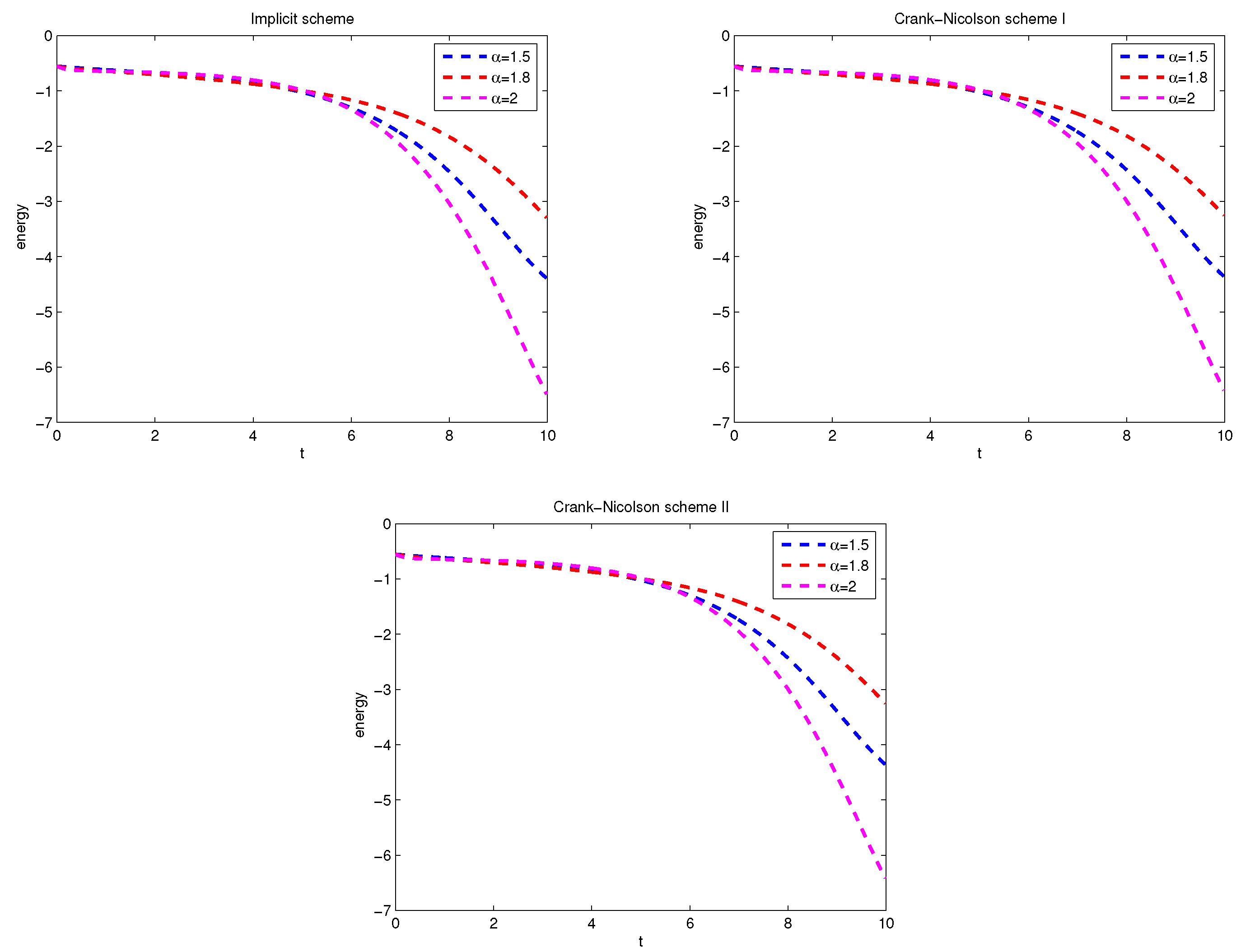
In this example, we consider fractional Allen-Cahn system (53)-(55), and show the wave form of the implicit scheme and Crank-Nicolson scheme by zero boundary condition. Consider initial value on or zero elsewhere, and we simulate the numerical solution with . Figure 7 and Figure 8 display the wave form of numerical solution at the difference and time. Figure 9 displays the the evolution of discrete energy over time by implicit scheme and Crank-Nicolson scheme. They also show that affects the propagation velocity of the solitary wave. For smaller , the propagation of the soliton got slower, thus indicating the presence of the quantum subdiffusion.
5. Conclusions
In the paper, we show the finite difference method and finite volume method for fractional diffuse equation with smooth and non-smooth solutions. The novelty of our method is that we formulated the fractional Laplacian operator as a weak singular integral, so as to avoid directly discretizing the hypersingular integral. Because of the solution of fractional diffusion equation is usually singular near the boundary, we give some numerical schemes including finite difference scheme and finite volume scheme to discrete fractional diffusion equation by fractional interpolation function. Moreover, it is find that the accuracy of the finite volume method is higher than that of the finite difference scheme, and the numerical error produces great turbulence for smaller s by finite difference scheme. Finally, several numerical examples are considered to demonstrate the validity and applicability of the numerical scheme to approximate fractional diffusion equations.
Funding
This work is supported by National Natural Science Foundation of China (No.12161070), Xing dian talent support project (No.XDYC-QNRC-2022-0038), Innovation team of Puer University (CXTD019), Scientific Research Fund Project of Yunnan Education Department (2022J0985).
References
- S. Samko, A. Kilbas and O. Marichev, Fractional Integral and Derivatives, Gordon and Breach Science Publishers, Yverdon, 1993. [CrossRef]
- S. Zhai, Z. Weng and X. Feng, Fast explicit operator splitting method and time-step adaptivity for fractional non-local Allen-Cahn model, Appl. Math. Model., 40 (2) (2016) 1315-1324. [CrossRef]
- N. Landkof, Foundations of Modern Potential Theory, Die Grundlehren der Mathematischen Wissenschaften 180, Springer-Verlag, New York, 1972.
- C. Li, F. Zeng, Numerical Methods for Fractional Calculus, Chapman and Hall/CRC, Boca Raton, 2015.
- F. Liu, P. Zhuang and Q. Liu, Numerical Methods and Applications of Fractional Partial Differential Equations, Science Press, China, 2015.
- Z. Sun and G. Gao, Finite Difference Methods for Fractional-order Differential Equations, Science Press, China, 2015.
- V. Tarasov, Fractional Dynamics: Applications of Fractional Calculus to Dynamics of Particles, Fields and Media, Springer, 2011.
- B. Guo, Fractional Partial Differential Equations and their Numerical Solutions, Science Press, China, 2011.
- S. Duo and Y. Zhang, Mass-conservative Fourier spectral methods for solving the fractional non-linear Schrödinger equation, Comput. Math. Appl., 71 (2016) 2257-2271. [CrossRef]
- P. Felmer, A. Quaas and J. Tan, Positive solutions of the nonlinear Schröinger equation with the fractional Laplacian, Proc. Roy. Soc. Edinburgh Sect. A, 142 (06) (2012) 1237-1262. [CrossRef]
- C. Celik, M. Duman, Crank-Nicolson method for the fractional diffusion equation with the Riesz fractional derivative, J. Comput. Phys., 231 (2012) 1743-1750. [CrossRef]
- G. Acosta, J. Borthagaray, O. Bruno, Regularity theory and high order numerical method for the (1D)-fractinal Laplacian, Math. Comput., 87 (312) (2018) 1821-1857.
- M. Li, C. Huang and P. Wang, Galerkin finite element method for nonlinear fractional Schrödinger equations, Numer. Algorithms, 74 (2017) 499-525.
- Y. Ran, J. Wang and D. Wang, On HSS-like iteration method for the space fractional coupled nonlinear Schrödinger equations, Appl. Math. Comput., 271 (2015) 482-488.
- Y. Ran, J. Wang and D. Wang, On preconditioners based on HSS for the space fractional CNLS equations, East Asian J. Appl. Math., 7 (2017) 70-81.
- M. Ran and C. Zhang, A conservative difference scheme for solving the strongly coupled nonlinear fractional Schrödinger equations, Commun. Nonlinear Sci. Numer. Simul., 41 (2016) 64-83.
- P. Wang and C. Huang, An energy conservative difference scheme for the nonlinear fractional Schr?dinger equations, J. Comput. Phys., 293 (2015) 238-251.
- P. Wang, C. Huang and L. Zhao, Point-wise error estimate of a conservative difference scheme for the fractional Schrödinger equation, J. Comput. Appl. Math., 306 (2016) 231-247.
- L. Wang, Y. Ma, L. Kong and Y. Duan, Symplectic Fourier pseudo-spectral schemes for Klein-Gordon-Schrödinger equations, China J. Comput. Phys., 28 (2011) 275-282.
- J. Wang and A. Xiao, An efficient conservative difference scheme for fractional Klein-Gordon-Schrödinger equations, Appl. Math. Comput., 320 (2018) 691-709.
- D. Wang, A. Xiao and W. Yang, Crank-Nicolson difference scheme for the coupled nonlinear Schr?dinger equations with the Riesz space fractional derivative, J. Comput. Phys. 242, 670- 681 (2013).
- H. Yang and A. Oberman,Numerical method for the fractional Laplacinal: a finite difference-quadrature approach, Siam: J.Numer.Anal., 52 (6) 3056-3084.
- S. Duo, H. WernervanWyk, Y. Zhang, A novel and accurate finite difference method for the fractional Laplacian and the fractional Poisson problem, J. Comput. Phys., 355 (2018) 233-252.
- T. Tang, H. Yuan, T. Zhou, Hermite spectral collocation methods for fractional PDEs in unbounded domains, Commun. Comput. Phys., 24 (4) (2018) 1143-1168 October 2018.
- Z. Mao and J. Shen, Hermite spectral methods for fractional PDEs in unbounded domains, to appear in SIAM J. Sci. Comput., 2017.
- T. Tang, L. Wang, H. Yuan, T. Zhou, Rational spectral methods for PDEs invoving fractional Laplacian unbounded domains.
- Y. Zhang, Z. Sun and H. Liao, Finite difference methods for the time fractional diffusion equation on non-uniform meshes, J. Comput. Phys., 265 (2014) 195-210.
- L. Zhao and W. Deng, High order finite difference methods on non-uniform meshes for space fractional operators, Advan. Comput. Math., 42 (2016) 425-468.
Figure 1.
The numerical errors and convergence rates of finite difference scheme
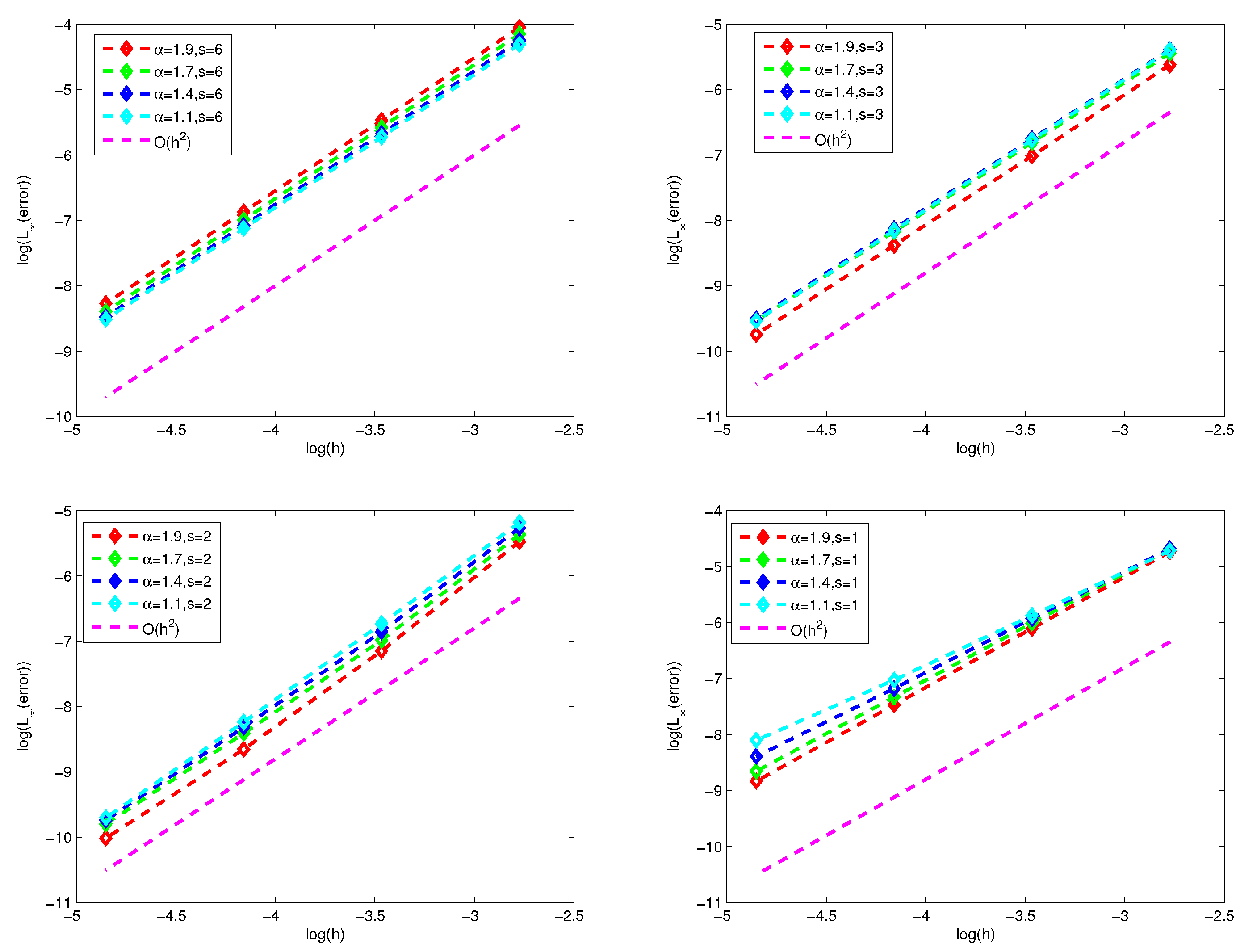
Figure 2.
The numerical errors and convergence rates of finite volume scheme
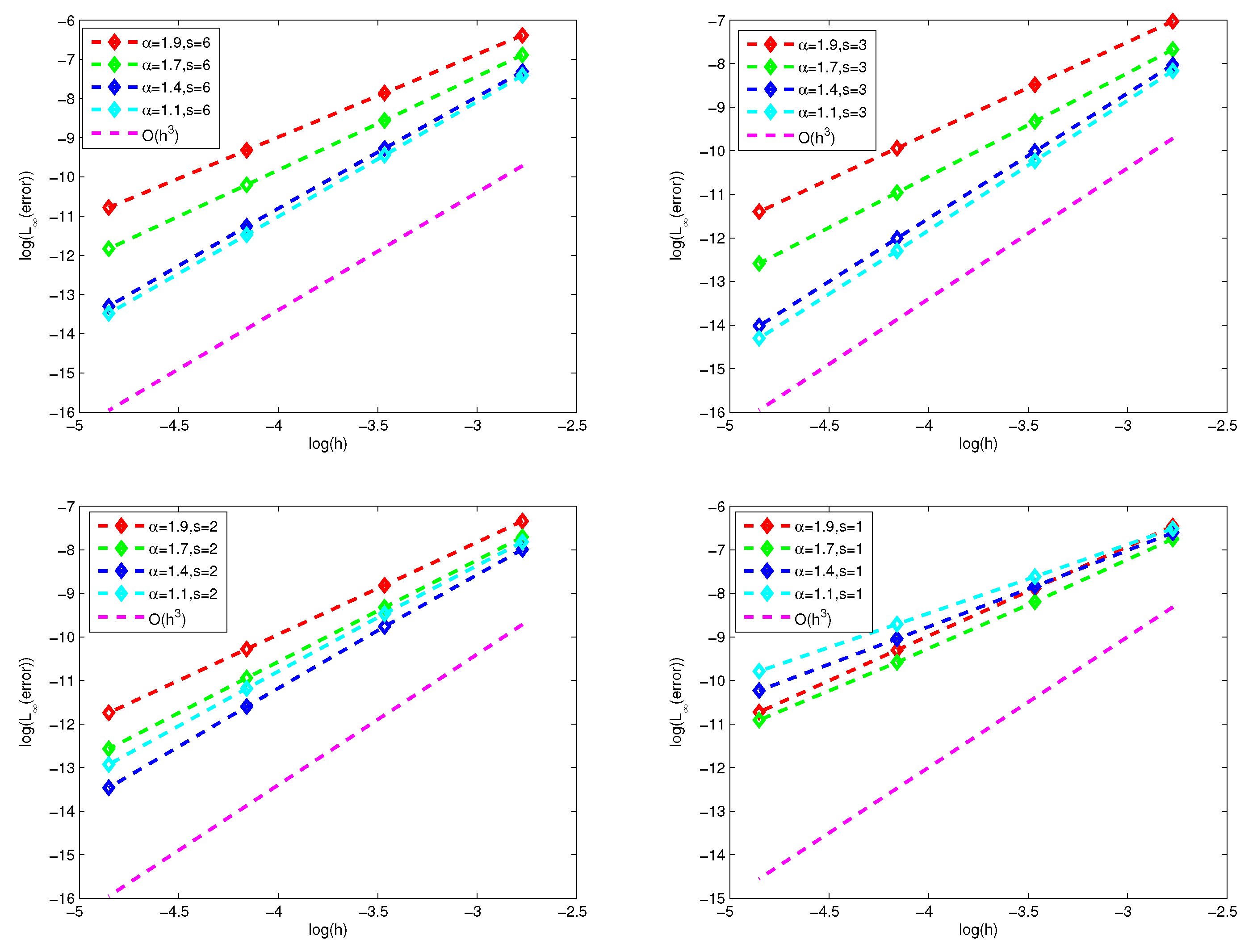
Figure 3.
The numerical errors of numerical solution for FDM I and FDM II
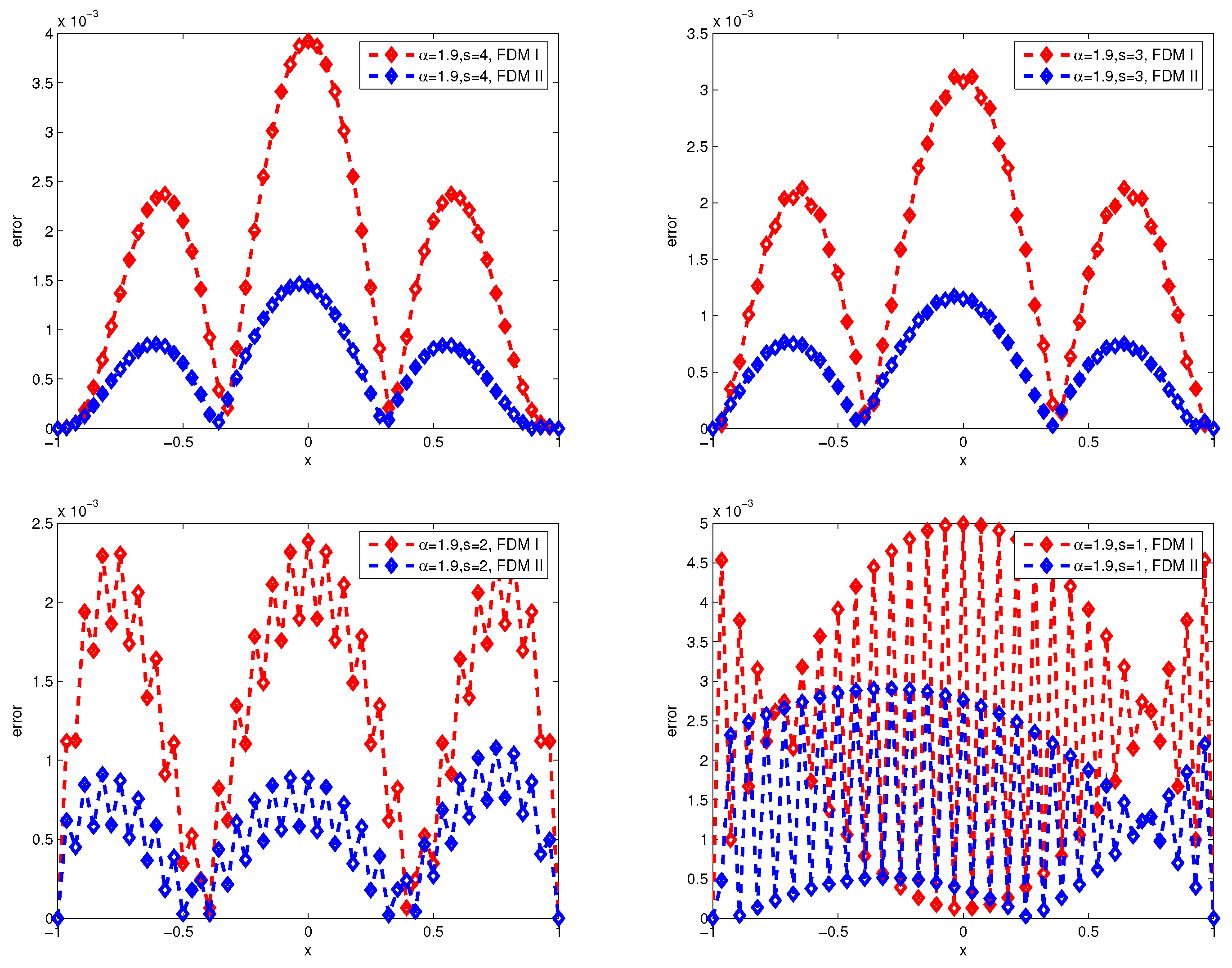
Figure 4.
The numerical errors of numerical solution for FDM I and FDM II
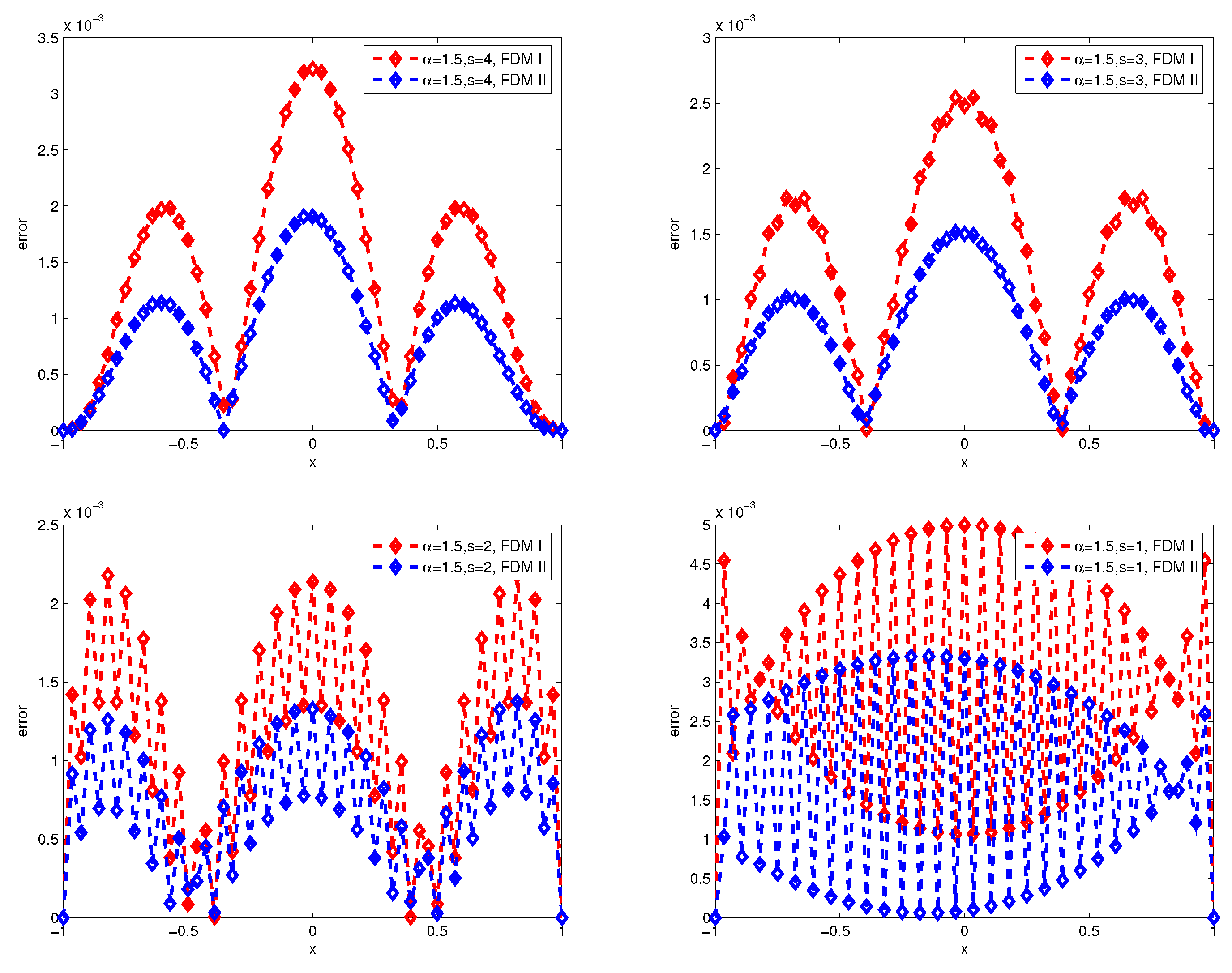
Figure 5.
The numerical errors of numerical solution for FVM I and FVM II
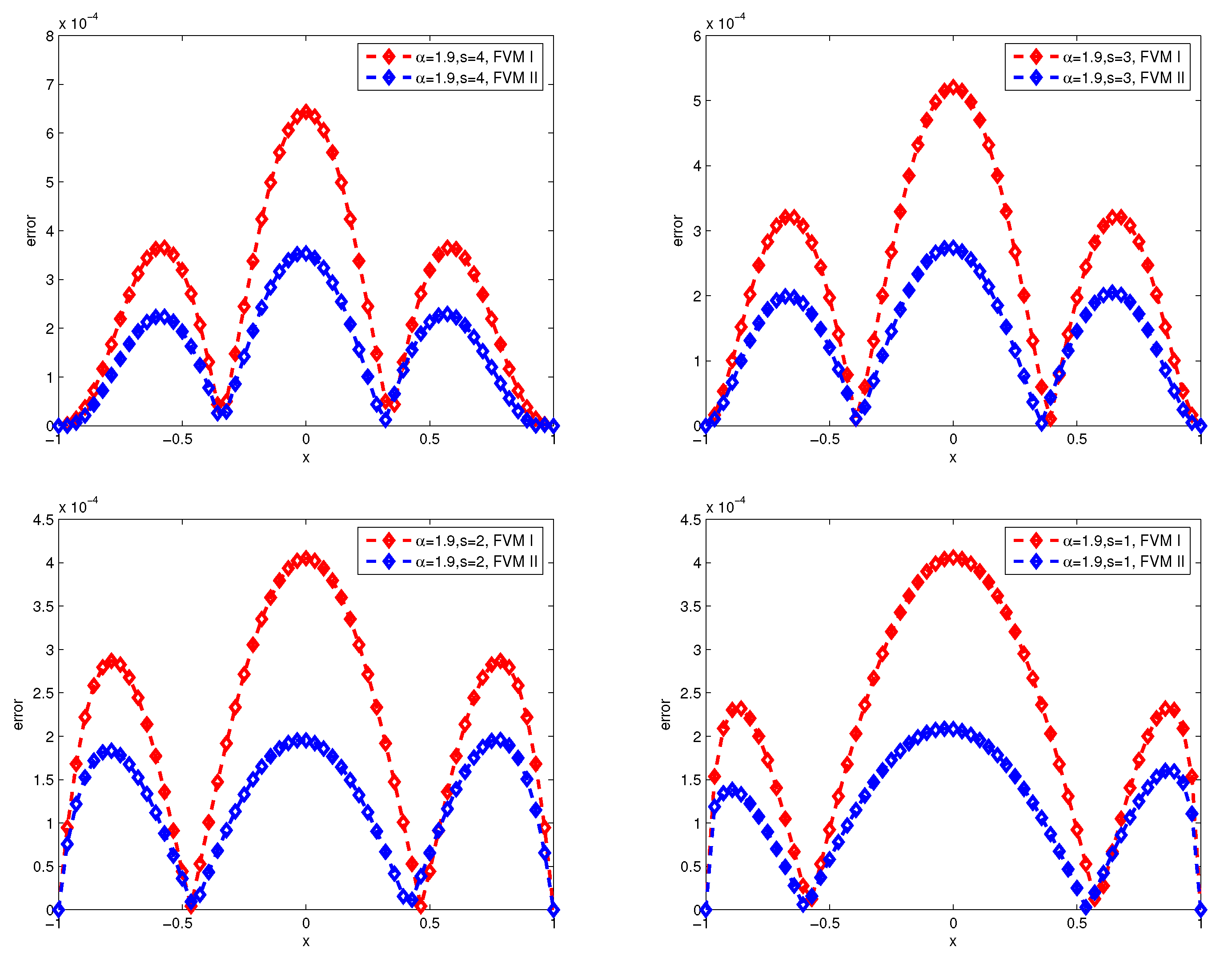
Figure 6.
The numerical errors of numerical solution for FVM I and FVM II
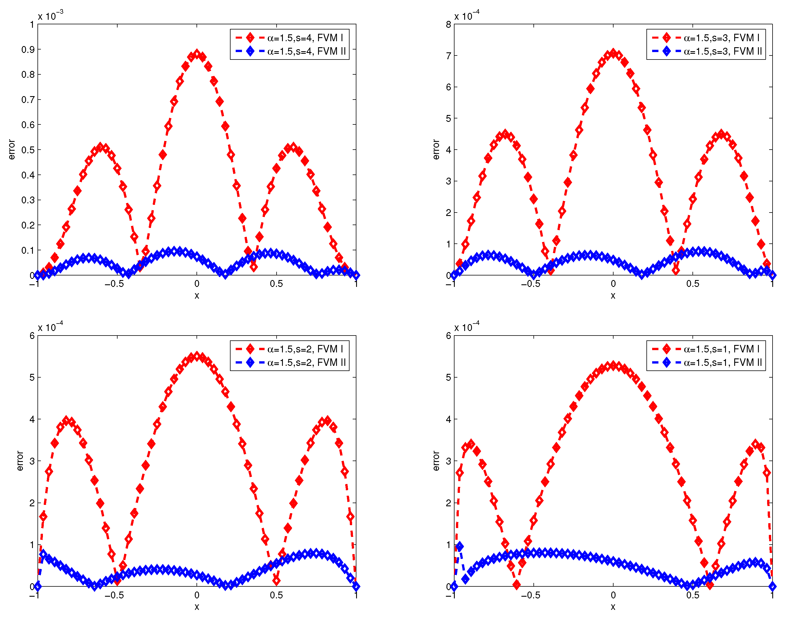
Figure 7.
The wave forms of the numerical solution with
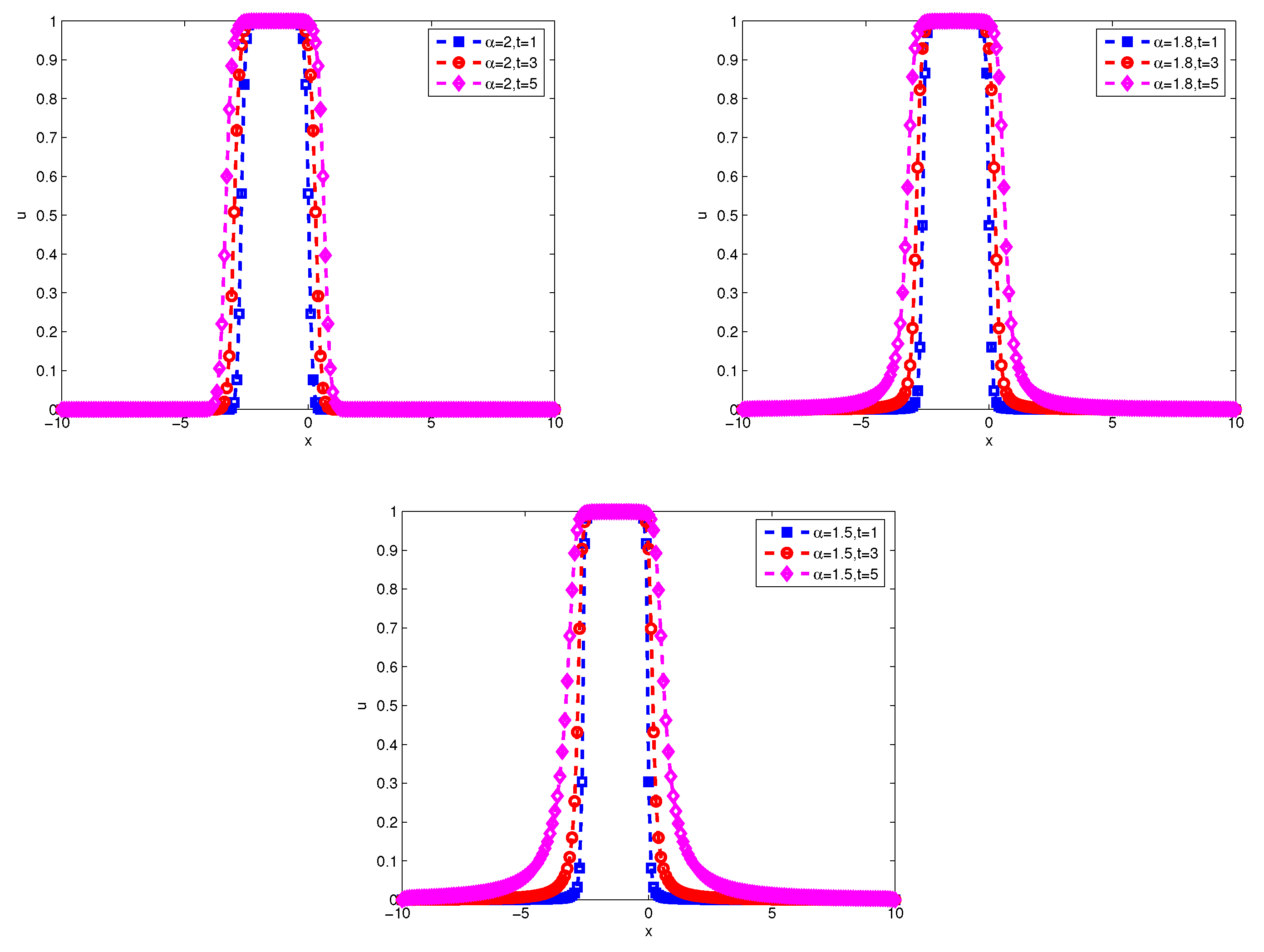
Figure 8.
The wave forms of the numerical solution with
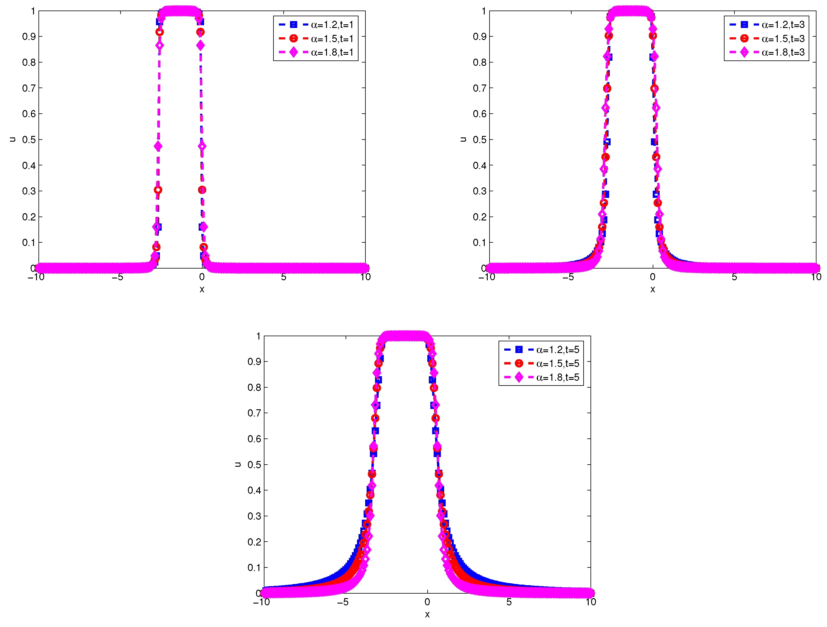
Figure 9.
The evolution of discrete energy over time
Disclaimer/Publisher’s Note: The statements, opinions and data contained in all publications are solely those of the individual author(s) and contributor(s) and not of MDPI and/or the editor(s). MDPI and/or the editor(s) disclaim responsibility for any injury to people or property resulting from any ideas, methods, instructions or products referred to in the content. |
© 2023 by the authors. Licensee MDPI, Basel, Switzerland. This article is an open access article distributed under the terms and conditions of the Creative Commons Attribution (CC BY) license (http://creativecommons.org/licenses/by/4.0/).
Copyright: This open access article is published under a Creative Commons CC BY 4.0 license, which permit the free download, distribution, and reuse, provided that the author and preprint are cited in any reuse.


