
Submitted:
23 April 2024
Posted:
24 April 2024
You are already at the latest version
Abstract
Regression models are highly popular in empirical research and come in many different forms to fit virtually any distribution, variable, or research question. Usually, these models also compute how much variation in the outcome variable can be explained by all predictors, which is relevant to understanding whether the predictors are, in sum, able to explain the outcome or whether other potentially unobserved factors are more relevant. This aspect is crucial for interventions and policy as even statistically significant regression coefficients can be meaningless if they have little influence on the outcome overall. Besides having a measurement to judge the overall goodness of fit, ranking predictors by their relative importance is also relevant. For such analyses, it is necessary to decompose the total explanatory power of a model and partition it so that each explanatory variable is assigned a share. This enables the computation of a predictor variable's absolute and relative influence. Dominance analysis is a statistical approach to achieve this goal.
Keywords:
dominance analysis
; regression
; variance decomposition
1. Why Do We Need Dominance Analysis?
Regression models are vastly popular in empirical
research. Researchers can choose from dozens of regression types depending on
the distribution of the dependent variable (the outcome). For continuous and
approximately normally distributed variables, linear models such as OLS
(ordinary least squares) are often the most appropriate. However, many more
potential models are available (binary logistic, ordered logistic, multinomial,
Poisson, etc.…). These models are also generalized and extended to work with panel
data (panel regressions) or clustered data (multilevel models) to suit many
research questions. Normally, these models also provide a measure of
statistical fit or goodness, which can be used to judge a model's overall
quality and validity. If the model fit is bad, the results reported by a model
might be meaningless. Hence, researchers are motivated to compute suitable
models with a good overall fit. For OLS models, the most popular measurement of
model fit is R², which is easy to compute and understand since it ranges from 0
to 1, with higher values indicating a better model fit. For R², this fit
directly translates to explained variation in the outcome. If R² is large, the
predictor variables can explain much variation in the outcome. This is
especially relevant for interventions and policy as it demonstrates that
changing certain variables will influence the outcome (if one believes the
regression model can be seen as a causal model, which is quite a different
question). Sometimes, R² is small, even if some or all variables in a model are
statistically highly significant, which is indicated by small p-values. In
these cases, making changes to the predictors might not be enough to influence
the outcome meaningfully as other, more relevant predictors are not observed,
and their influence remains unclear.
When multiple predictors are in a regression model,
and R² is large, researchers are often interested in decomposing this total
explained variance to understand better which predictor is the most relevant.
By doing so, predictors can be ranked by their importance or influence. This enables
researchers to state which predictors are the most promising for a potential
intervention. Dominance analysis (DA) is a statistical approach to achieve this
goal (Azen & Budescu, 2006; Budescu, 1993). DA enables researchers to
disentangle the total explained variation in the outcome and assign a share of
explained variance to each predictor variable. While the approach is
statistically simple, it can be a challenge to compute if the datasets are
large or if there are many predictors included. This draft will give a short
and intuitive explanation of how DA works.
2. A Simple Example
Assume one outcome variable (y) and three
independent variables (predictors; x1, x2, x3). In the most basic case, these
explanatory variables are uncorrelated with each other (while this can be
tested easily, it is usually not the case). We assume all four variables are
continuous and approximately normally distributed, so OLS is the appropriate
modeling choice. We compute a model that includes all three predictors to
compute the total variation explained by all predictors. This can be visualized
as follows (Figure 1):
The total explained variance is the sum of the
intersections with the y-circle. The share that is explained by x1 alone is
shown in red. Let us give a numerical example. First, we compute a correlation
matrix to demonstrate that the three predictors are uncorrelated (Table 1, N = 15,000).
As we see, while each explanatory variable is correlated with the dependent variable, they are uncorrelated with each other. In this simple case, the decomposition of the total explained variance is simple. After having computed a model with all three predictors, we compute three additional ones where only one predictor is included. We can summarize this as follows (Table 2).
We report unstandardized regression coefficients and R² for each model from M1 to M4. As we can see, the total R², shown in M4, is just the sum of the R² values from M1 to M3 (except for rounding errors). Decomposing the importance of the predictors is straightforward. As absolute importance is already reported in the table, the relative one is easy to compute (for x1, it is 0.246 / 0.749, which is 0.328 or about 33% of the total explained variance by the model.
3. Correlated Predictors
However, as soon as predictors are correlated, ranking them becomes a challenge. Suppose we have other data and the following correlation matrix (Table 3, N = 15,000):
If we were to compute the same regression models as before, we would note that the R² would not add up to the total share, reported by the saturated model (M7, Table 4) with all three predictors. This is because the explanatory variables now share explained variance. We can visualize this as follows (Figure 2):
Since x1, x2, and x3 overlap, three regression models are insufficient to decompose the total variance. Before starting, we note that each explanatory variable still has a share of explained variance that is unique to it, meaning that no other variable explains this part. For x1, this share is depicted in red. However, reporting only this part, the uniquely explained variance by each explanatory variable is usually insufficient. It ignores the shared variances, meaning that the unique shares never sum up to the total R² of the saturated model, which is unsatisfactory. DA helps us solve the problem.
4. How Does Dominance Analysis Work?
The idea of DA is to form all possible combinations of all predictors and use each set in a separate regression. By doing so, the share unique to each predictor can be summed up and averaged over all potential models. While this is potentially much work, it is a highly flexible approach that works with virtually any regression model or fit statistic. Before discussing the benefits and downsides, let us continue with the numerical example. Note that three predictors form a set of all potential combinations as follows: A | B | C | A+B | A+C | B+C. The saturated model (A+B+C) is only useful for computing the variance that is explained by all predictors together. For three predictors, we need to compute a total of seven models. We have done that and report the results in Table 4.

Table 4.
Regression table (correlated predictors).
| M1 | M2 | M3 | M4 | M5 | M6 | M7 | |
|---|---|---|---|---|---|---|---|
| x1 | 1.685*** | 1.561*** | 0.852*** | 0.976*** | |||
| x2 | 1.392*** | 1.236*** | 0.904*** | 0.989*** | |||
| x3 | 1.899*** | 1.388*** | 1.628*** | 1.017*** | |||
| R² | 0.478 | 0.326 | 0.607 | 0.732 | 0.685 | 0.732 | 0.833 |
* p < 0.05, ** p < 0.01, *** p < 0.001.
We will demonstrate how to compute the relative importance of x1 in the following numerical example. As we can see, x1 is included in four models (M1, M4, M5, M7). We compute the share of unique additional variance by x1 for each model and average the results separately by the total number of predictors. As a visual aid, we can utilize Figure 3.
In the upper left corner, we see that there is one model in which x1 is the sole predictor. This corresponds to M1. The unique share of variance explained by x1 is 0.478. Next, we continue with the two models on the right side of the figure, where exactly two variables are present. In both cases, we must subtract the share from the other variable to arrive at the unique share by x1. This is 0.732 – 0.326 = 0.406 and 0.685 – 0.607 = 0.078. Since these are all models with exactly two variables, we form the arithmetic mean of both values (0.406 + 0.078) / 2 = 0.242. Finally, we go to the model with three predictors. Again, we want to compute the share in red by taking the total explained variance and removing the share from x2 and x3. For this, we need models M7 and M6. The unique share of x1 is 0.833 – 0.732 = 0.101. We have now computed the explanatory power unique to x1 for all subsets. Now we average these results: (0.478 + 0.242 + 0.101) / 3 = 0.274. This gives the final result, which is the part of the total explained variance we can assign to x1. If we repeat these computations for x2 and x3, we get their values: 0.221 and 0.338. If we add these shares, we arrive at the total explained variance (reported in M7): 0.833. We have successfully decomposed the explained variances, so it is clear which variable contributes the most (x3) and the least (x2). If desired, we could also standardize these shares to add up to 100%.
4. Advantages of Dominance Analysis
As we have just demonstrated, conducting DA is simple and only requires the computation of the original regression model with subsets of predictor variables. This routine is implemented in many modern statistical software packages, as shown below. The second main benefit is that this approach is highly flexible. While we have used OLS models and R² for a demonstration, it is simple to generalize the approach to virtually any fit measure. For example, in logistic regression models, we could use Pseudo-R² instead. Other model fit measures, such as AIC or BIC, and can also be utilized to be even more general. As long as the statistic of the model fit is reported by a regression model, we can decompose it. Some caution is necessary when using statistics such as adjusted R², computed by adding information on the number of predictors. This can mean the decomposed shares do not add to the total.
5. Downsides of Dominance Analysis
The main problem with DA is that computational requirements grow exponentially with the number of predictors. The general rule is that 2p-1 models are required, where p is the number of predictor variables used. We need 1,023 regression models for ten predictors, for 15 already 32,767, and for 20 more than a million. Even modern systems cannot compute DA if the number of predictors is very large. One solution is to simplify the models or group predictors as sets. For example, assume that your model has 20 predictors. However, five of these predictors measure a person's health, and six measure a person's financial means. If one groups the predictors as such, the total number of models is reduced from more than a million to only 2,047. This can also be beneficial for the interpretation as one can interpret the health influences together.
It's crucial to approach causal analysis and interpretations with caution when it comes to DA. Contrary to popular belief, DA does not possess a magical ability to render your results causal. Similar to a standard regression model, introducing additional variables to the model can help approximate causal effects by ruling out confounding (Pearl, 2009). However, it's important to remember that the primary aim of DA is not to estimate causal effects but to decompose variances, which can lead to interpretations that are entirely distinct from a causal perspective.
6. Inference
If one wants to compare the decomposed shares rigorously, more than DA is required. Suppose one variable explains 21% of the total variance, and a second predictor explains 23%. While the point estimate for variable two is higher, it remains to be seen whether this difference is statistically significant (that means whether one can generalize the findings from the sample to the population). To enable such statements, DA can be combined with bootstrapping or the jackknife, which are forms of resampling (Bittmann, 2021; Efron & Tibshirani, 1994). Bootstrapping generates confidence intervals for each share. If these intervals do not overlap, one can state that the shares are statistically different. One form to visualize this is as follows (example with five predictors):
Figure 4.
Computing confidence intervals enables statistical inference.
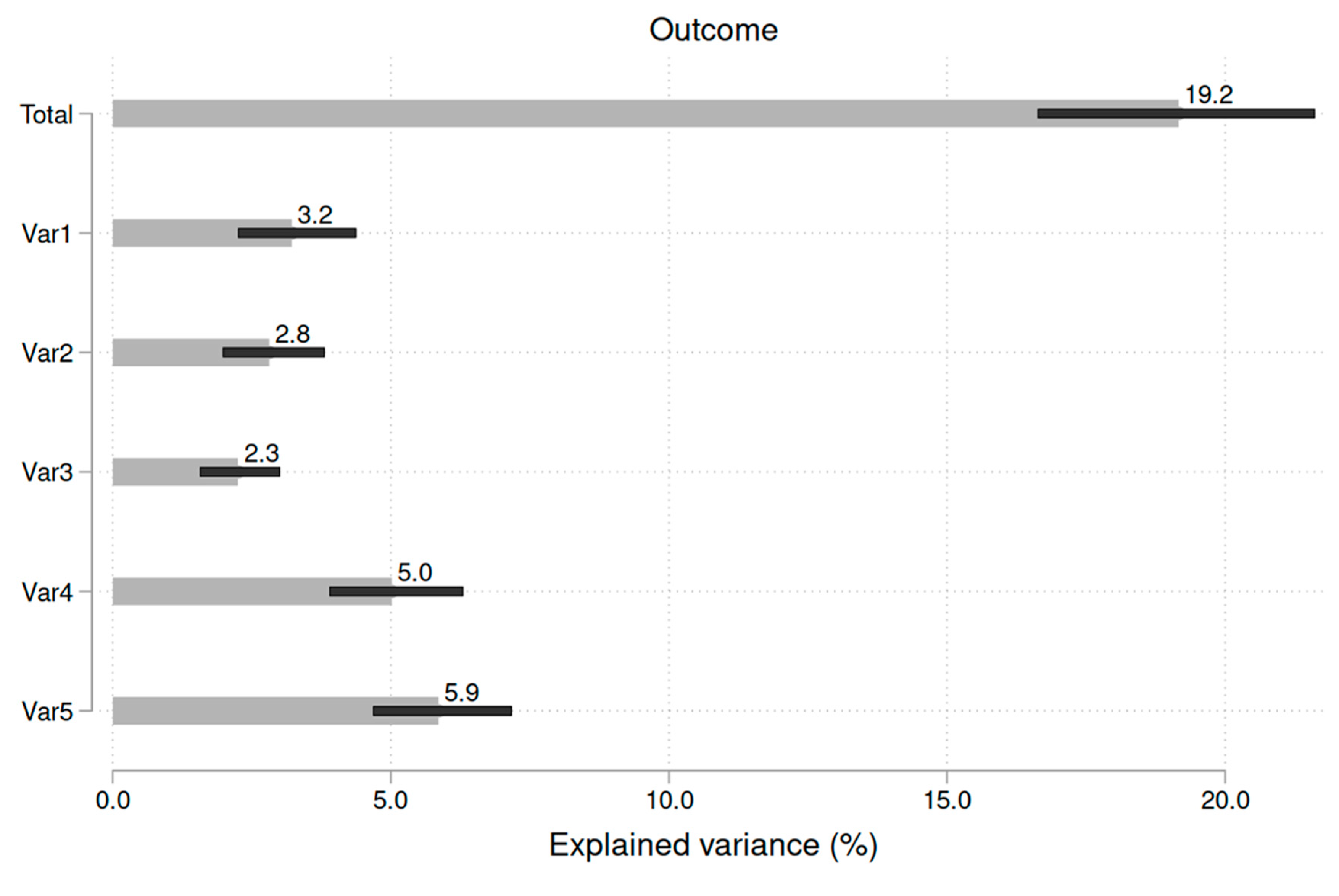
As we see, Var5 explains more variance than Var3. Since these 95% confidence intervals do not overlap, the difference between the two variables is statistically significant on the 5% level. However, as the confidence intervals overlap between Var4 and Var5, this difference is statistically insignificant.
7. Software Implementations
- Stata provides the package domin (Luchman, 2021).
- R provides the package domir (https://cran.r-project.org/web/packages/domir/vignettes/domir_basics.html)
- SPSS also has solutions available (Lorenzo-Seva et al., 2010).
References
- Azen, R., & Budescu, D. V. (2006). Comparing Predictors in Multivariate Regression Models: An Extension of Dominance Analysis. Journal of Educational and Behavioral Statistics, 31(2), 157–180. [CrossRef]
- Bittmann, F. (2021). Bootstrapping: An Integrated Approach with Python and Stata (1st ed.). De Gruyter. [CrossRef]
- Budescu, D. V. (1993). Dominance analysis: A new approach to the problem of relative importance of predictors in multiple regression. Psychological Bulletin, 114(3), 542.
- Efron, B., & Tibshirani, R. J. (1994). An introduction to the bootstrap. CRC press.
- Lorenzo-Seva, U., Ferrando, P. J., & Chico, E. (2010). Two SPSS programs for interpreting multiple regression results. Behavior Research Methods, 42(1), 29–35. [CrossRef]
- Luchman, J. N. (2021). Determining relative importance in Stata using dominance analysis: Domin and domme. The Stata Journal: Promoting Communications on Statistics and Stata, 21(2), 510–538. https://doi.org/10.1177/1536867X211025837. [CrossRef]
- Pearl, J. (2009). Causality. Cambridge University Press.
Figure 1.
Explained variance by three uncorrelated predictors (x1, x2, x3).
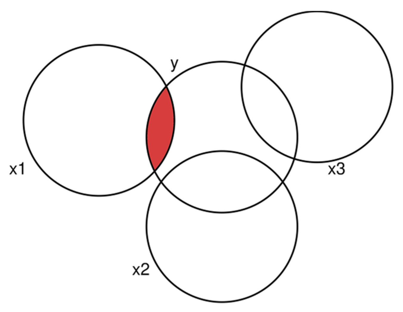
Figure 2.
Variance decomposition by three correlated predictors. The red area is the share of variance that is unique to x1.
Figure 2.
Variance decomposition by three correlated predictors. The red area is the share of variance that is unique to x1.
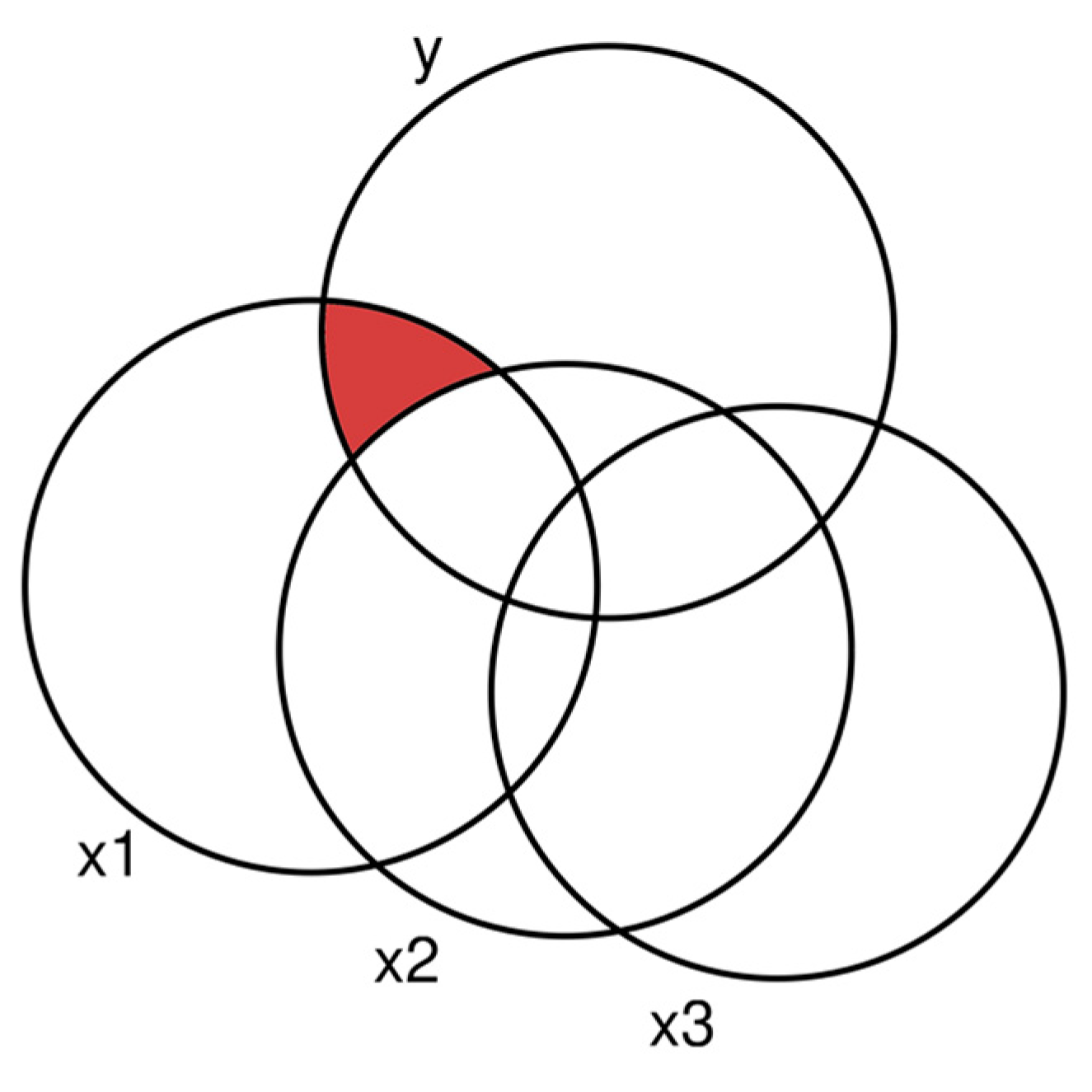
Figure 3.
All models to consider to compute the contribution of x1.
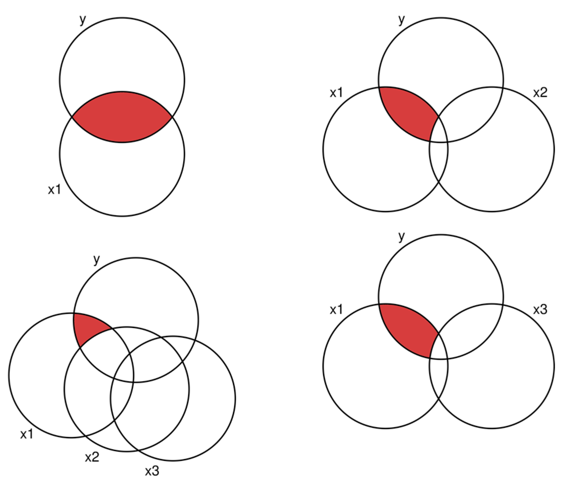
Table 1.
Correlation matrix (uncorrelated predictors).
| y | x1 | x2 | x3 | |
|---|---|---|---|---|
| y | 1 | |||
| x1 | 0.496*** | 1 | ||
| x2 | 0.501*** | 0.00523 | 1 | |
| x3 | 0.508*** | -0.00586 | 0.0120 | 1 |
* p < 0.05, ** p < 0.01, *** p < 0.001.
Table 2.
Regression table (uncorrelated predictors).
| M1 | M2 | M3 | M4 | |
|---|---|---|---|---|
| x1 | 0.989*** | 0.989*** | ||
| x2 | 1.005*** | 0.988*** | ||
| x3 | 1.010*** | 1.004*** | ||
| R² | 0.246 | 0.251 | 0.258 | 0.749 |
* p < 0.05, ** p < 0.01, *** p < 0.001.
Table 3.
Correlation matrix (correlated predictors).
| y | x1 | x2 | x3 | |
|---|---|---|---|---|
| y | 1 | |||
| x1 | 0.695*** | 1 | ||
| x2 | 0.572*** | 0.100*** | 1 | |
| x3 | 0.774*** | 0.600*** | 0.300*** | 1 |
* p < 0.05, ** p < 0.01, *** p < 0.001.
Disclaimer/Publisher’s Note: The statements, opinions and data contained in all publications are solely those of the individual author(s) and contributor(s) and not of MDPI and/or the editor(s). MDPI and/or the editor(s) disclaim responsibility for any injury to people or property resulting from any ideas, methods, instructions or products referred to in the content. |
© 2024 by the authors. Licensee MDPI, Basel, Switzerland. This article is an open access article distributed under the terms and conditions of the Creative Commons Attribution (CC BY) license (http://creativecommons.org/licenses/by/4.0/).
Copyright: This open access article is published under a Creative Commons CC BY 4.0 license, which permit the free download, distribution, and reuse, provided that the author and preprint are cited in any reuse.


