Submitted:
14 April 2025
Posted:
16 April 2025
Read the latest preprint version here
Abstract
We present a reformulation of fundamental physics, transitioning from an enumeration of independent axioms to the solution of a single optimization problem derived from the structure of experiments. Any experiment comprises an initial preparation, a physical evolution, and a final measurement. Grounded in this structure, we determine the final measurement distribution by minimizing its entropy relative to its initial preparation distribution, subject to a natural constraint. Solving this optimization problem identifies a unified theory encompassing quantum mechanics, general relativity (acting on spacetime geometry), and Yang-Mills gauge theories (acting on internal spaces). Notably, consistency requirements restrict valid solutions to 3+1 dimensions, thus deriving spacetime dimensionality. This reformulation suggests that the established laws of physics, including their specific forces, symmetries, and dimensionality, emerge naturally from the requirement of the minimal informational change from preparation to measurement, consistent with the natural constraint.
Keywords:
foundations of physics
1. Introduction
Statistical mechanics (SM), in the formulation developed by E.T. Jaynes [1,2], is founded on an entropy optimization principle. Specifically, the Boltzmann entropy is maximized under the constraint of a fixed average energy :
The Lagrange multiplier equation defining the optimization problem is:
where and are Lagrange multipliers enforcing the normalization and average energy constraints. Solving this optimization problem yields the Gibbs measure:
where is the partition function.
For comparison, quantum mechanics (QM) is not formulated as the solution to an optimization problem, but rather consists of a collection of axioms[3,4]:
- QM Axiom 1 of 5
- State Space: Every physical system is associated with a complex Hilbert space, and its state is represented by a ray (an equivalence class of vectors differing by a non-zero scalar multiple) in this space.
- QM Axiom 2 of 5
- Observables: Physical observables correspond to Hermitian (self-adjoint) operators acting on the Hilbert space.
- QM Axiom 3 of 5
- Dynamics: The time evolution of a quantum system is governed by the Schrödinger equation, where the Hamiltonian operator represents the system’s total energy.
- QM Axiom 4 of 5
- Measurement: Measuring an observable projects the system into an eigenstate of the corresponding operator, yielding one of its eigenvalues as the measurement result.
- QM Axiom 5 of 5
- Probability Interpretation: The probability of obtaining a specific measurement outcome is given by the squared magnitude of the projection of the state vector onto the relevant eigenstate (Born rule).
Physical theories have traditionally been constructed in two distinct ways. Some, like QM, are defined through a set of mathematical axioms that are first postulated and then verified against experiments. Others, like SM, emerge as solutions to optimization problems with experimentally-verified constraints.
We propose to generalize the optimization methodology of E.T. Jaynes to encompass all of physics, aiming to derive a unified theory from a single optimization problem.
To that end, we introduce the following constraint:
Axiom 1
(Nature).
where are matrices, and is their average.
This constraint, as it replaces the scalar with the matrix , extends E.T. Jaynes’ optimization method to encompass non-commutative observables and symmetry group generators required for fundamental physics.
We then construct an optimization problem:
Definition 1
(Physics). Physics is the solution to:
where λ and t are Lagrange multipliers enforcing the normalization and natural constraints, respectively.
This definition constitutes our complete proposal for reformulating fundamental physics—no additional principles will be introduced. By replacing the Boltzmann entropy with the relative Shannon entropy, the optimization problem extends beyond thermodynamic variables to encompass any type of experiment. This generalization occurs because relative entropy captures the essence of any experiment: the relationship between a final measurement and its initial preparation.
Two key constraints shape our framework. The normalization constraint ensures we are working with a proper predictive theory, while the natural constraint spawns the domain of applicability of the theory. The crucial insight is that because our formulation maintains complete generality in the structure of experiments while optimizing over all possible predictive theories, the resulting solution holds true, by construction, for all realizable experiments within its domain.
This approach reduces our reliance on postulating axioms through trial and error, and simplifies the foundations of physics. Specifically, when we employ the natural constraint—the most permissive constraint for this problem (see Discussion for proof)—, the solution spawns its largest domain, pointing towards a unified physics where fundamental theories emerge naturally—e.g. SM when , QM when , and general relativity (acting on spacetime) + Yang-Mills (acting on internal spaces) when . As we found, these three solutions are the only possible ones, as those entailed by other algebras encounter obstructions which violates the axioms of probability theory.
Theorem 1.
The general solution of the optimization problem is:
Proof.
We solve the entropy minimization problem by setting the derivative of the Lagrange multiplier equation with respect to to zero:
Normalizing the probabilities using , we find:
Substituting back, we obtain:
then using the identity for square matrices , we get:
□
As we will see in the results section, this solution encapsulates three distinct special cases:
- Statistical Mechanics: To recover SM from Equation 10, we consider the case where the matrices are , i.e., real scalars. Specifically, we set:and take to be a uniform distribution. Then, Equation 10 reduces to the Gibbs distribution:where t corresponds to the of SM. This demonstrates that our solution generalizes SM, as it recovers it when are scalars.
-
Quantum Mechanics: By choosing to represent the algebra, we derive the axioms of QM from optimization. Specifically, we set:In the results section, we will detail how this choice leads to the the Born rule in lieu of the Gibbs measure, and that the partition function is unitary invariant—the solution is shown to satisfy all five axioms of QM.
- Unified Theory: Extending our approach, we choose to be matrices representing the algebra. Specifically, we consider multivectors of the form , where is a bivector and is a pseudoscalar of the 3+1D geometric algebra . The matrix representation of is:where , and b correspond to the generators of the group, which includes both Lorentz boosts/rotations and the four-volume orientation. Solving the optimization problem with this choice leads to a relativistic quantum probability measure extending the Born rule from to . The solution is shown to uniquely satisfy both general relativity (acting on spacetime) and Yang-Mills (acting on its internal spaces).
-
Dimensional Obstructions: Definition 1 yields valid probability measures only in specific cases of Axiom 1. Beyond the instances of statistical mechanics and quantum mechanics, Axiom 1 produces a consistent solution only in 3+1 dimensions. In other dimensional configurations, various obstructions arises violating the axioms of probability theory. The following table summarizes the geometric cases and their obstructions:where means the geometric algebra of dimensions, where p is the number of positive signature dimensions and q of negative signature dimensions. QM shows up twice because both and the even-subalgebra of are isomorphic to .We will first investigate the unobstructed cases in Section 2.1, Section 2.2 and Section 2.3 and then demonstrate the obstructions in Section 2.4. These obstructions are desirable because they automatically limit the theory to 3+1D, thus providing a built-in mechanism for the observed dimensionality of our universe.
2. Results
2.1. -constraint: Quantum Mechanics
In SM, the central observation is that energy measurements of a thermally equilibrated system tend to cluster around a fixed average value (Equation 1). In contrast, QM is characterized by the presence of interference effects in measurement outcomes. To capture these features, we introduce the following special case of Axiom 1:
Definition 2
( constraint).We reduce the generality of Axiom 1 to the generator of the group. Specifically, we replace
where are scalar values (e.g., energy levels), are the probabilities of outcomes, the matrices generate the group, and where and .
Then, the Lagrange multiplier equation (Definition 1) becomes:
The general solution of the optimization problem (Theorem 1), with the above-mentioned replacements, reduces to the following ensemble:
Though initially unfamiliar, this form effectively establishes a comprehensive formulation of QM, as we will demonstrate.
Let us introduce a definition for . Since is a real number equal or greater than 0, it means that is a structure whose determinant is positive. Furthermore, the evolution operator must preserve this structure when acting on it. These two requirements means that . We also note that , and that and . Consequently, we can reposition inside the determinant where it becomes :
In this matrix representation, the determinant is equivalent to the complex norm. Replacing the former with the later yields:
This equation describes the time-evolution of a quantum system in its eigenvector: where is the expected outcome. The full gamut of unitary evolution is obtained as a property of the ensemble, which is unitary invariant. In fact, the partition function is a map , and as such it defines the inner product of a n-dimensional Hilbert space. This relationship is articulated as follows:
where
Furthermore, since is unitary invariant, this relation generalizes as follows, by any change of basis :
Thus yielding the general solution:
Let us now investigate how the axioms of QM are recovered from this result:
- The entropy maximization procedure inherently normalizes physical states with . Furthermore, as physical states associate to the probability measure, and the probability is defined up to a phase, we conclude that physical states map to Rays within Hilbert space. This demonstrates QM Axiom 1 of 5.
-
An observable of the ensemble must satisfy:Since , then any self-adjoint operator satisfying the condition will equate the above equation, simply because . This demonstrates QM Axiom 2 of 5.
- The system’s dynamics emerge from differentiating Equation 39 with respect to the Lagrange multiplier. This is manifested as:which is the Schrödinger equation. This demonstrates QM Axiom 3 of 5.
-
From Equation 39 it follows that the possible microstates of the system correspond to specific eigenvalues of . An observation can thus be conceptualized as sampling from , with the measured state being the occupied microstate i. Consequently, when a measurement occurs, the system invariably emerges in one of these microstates, which directly corresponds to an eigenstate of . Measured in the eigenbasis, the probability measure is:In scenarios where the probability measure is expressed in a basis other than its eigenbasis, the probability of obtaining the eigenvalue is given as a projection on a eigenstate:Here, signifies the squared magnitude of the amplitude of the state when projected onto the eigenstate . As this argument hold for any observable, this demonstrates QM Axiom 4 of 5.
- Finally, since the probability measure (Equation 35) replicates the Born rule, QM Axiom 5 of 5 is also demonstrated.
These results show that the -constraint is sufficient to entail the foundations of QM through the principle of relative entropy minimization.
2.2. -constraint: Euclidean QM in 2D
In this section, we investigate a model, isomorphic to QM, that lives in 2D—it provides a valuable starting point before addressing the more complex 3+1D case. Since , then this model is isomorphic to QM. Before we solve the optimization problem, we will first define the determinant of a multivector of .
2.2.1. Multivector Determinant
In general a multivector of can be written as , where a is a scalar, is a vector and a pseudo-scalar, can be represented as a real matrix via an isomorphism:
Definition 3
(Pauli Algebra Isomorphism). The map defined by:
extends linearly and multiplicatively to an isomorphism between and the algebra of real matrices. In particular, the basis bivector maps to:
Definition 4
(Matrix Representation). For a multivector , its matrix representation under φ is:
We now introduce the multivector conjugate, also known as the Clifford conjugate, which generalizes the concept of complex conjugation to multivectors.
Definition 5
(Multivector Conjugate—in ).Let be in . Then its multivector conjugate is defined as:
The determinant of the matrix representation of a multivector can be expressed as a multivector self-product:
Theorem 2
(Multivector Determinant—in ).Let be in , then:
Proof.
Let thus . Then:
□
2.2.2. Inner Product
Building upon the concept of the multivector conjugate, we introduce the multivector conjugate transpose, which serves as an extension of the Hermitian conjugate to the domain of multivectors.
Definition 6
(Multivector Conjugate Transpose). Let :
The multivector conjugate transpose of is defined as first taking the transpose and then the element-wise multivector conjugate:
Definition 7
(Bilinear Form). Let and be two vectors valued in :
We introduce the following bilinear form:
Theorem 3
(Inner Product). Restricted to the even sub-algebra of , the bilinear form is an inner product.
Proof.
This is isomorphic to the inner product of a complex Hilbert space, with the identification where corresponds to i. □
2.2.3. The Optimization Problem
The -constraint is recovered by posing and then reduces as follows:
The fundamental Lagrange Multiplier Equation:
where
- and are the Lagrange multipliers
- are the multivectors of , reduced by and
- the factor (1/2) is there to regularize the adjoint action on a vector
It yields the following solution:
where .
As with the -constraint case, the partition function defines the inner product of a n-dimensional Hilbert space. The wavefunction is:
Definition 8
(-valued Wavefunction).
where .
The dynamics are described by a variant of the Schrödinger equation, which is derived by taking the derivative of the wavefunction with respect to the Lagrange multiplier, :
Definition 9
(-valued Schrödinger Equation).
Since , then it should come to no surprise that the theory resulting from the -constraint is of the same mathematical form as QM, obtained from the -constraint.
One difference however, is that we gain these extra structures:
Definition 10
(David Hestenes’ Formulation). In 3+1D, the David Hestenes’ formulation [5] of the wavefunction is , where is a Lorentz boost or rotation and where is a phase. In 2D, as the algebra only admits a bivector, his formulation would reduce to , where ρ is a probability density and R is a Spin(2)-valued rotor—this is the form we have recovered:
The definition of the Dirac current applicable to our wavefunction follows the formulation of David Hestenes:
Definition 11
(Dirac Current). The Dirac current for the 2D theory is defined as:
where is a -rotated basis vector.
2.3. -constraint: Gravity + Yang-Mills
Extending the framework to relativistic quantum mechanics begins by considering a measurement constraint having a -phase symmetry. This allows for transformations that include boosts and rotations, and re-orientations (David Hestene describes "re-orientation" as representing the changing orientation of the spin plane due to Zitterbewegung). We begin with a definition of the determinant for a multivector of .
2.3.1. The Multivector Determinant
As we did in the beginning of the 2D case, our goal here will be to express as a multivector self-product. To achieve that, we begin by defining a general multivector in the geometric algebra :
where a is a scalar, a vector, a bivector, is pseudo-vector and a pseudo-scalar. Explicitly,
Definition 12
(Real-Majorana Algebra Isomorphism). The map defined by:
extends linearly and multiplicatively to an isomorphism between and the algebra of real matrices.
Definition 13
(Matrix Representation).
To manipulate and analyze multivectors in , we introduce several important operations, such as the multivector conjugate, the pseudo-blade conjugate, and the multivector determinant.
Definition 14
(Multivector Conjugate—in ).
Definition 15
(Pseudo-Blade Conjugate—in ). The pseudo-blade conjugate of is
Lundholm[6] proposes a number the multivector norms, and shows that they are the unique forms which carries the properties of the determinants such as to the domain of multivectors:
Definition 16.
The self-products associated with low-dimensional geometric algebras are:
where is a conjugate that reverses the sign of pseudo-scalar blade (i.e. the highest degree blade of the algebra).
We can now express the determinant of the matrix representation of a multivector via a self-product. This choice is unique:
(3,1)).Theorem 4 (The Multivector Determinant—in GA
Proof.
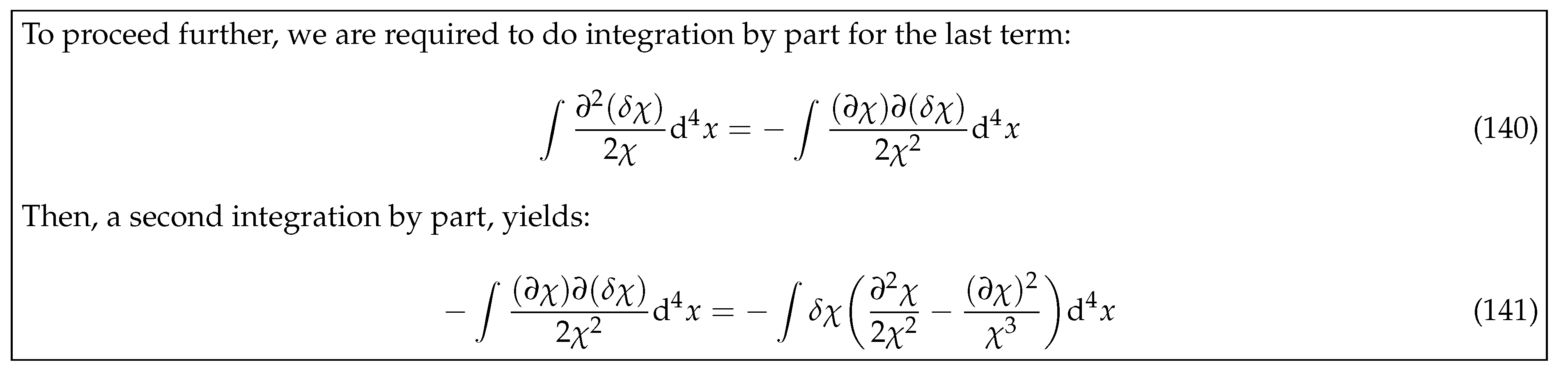
Please find a computer assisted proof of this equality in Annex F. □
As can be seen from this theorem, the relationship between determinants and multivector products becomes more sophisticated in 3+1D. Unlike the 2D case where the determinant could be expressed using a product of two terms, in the determinant requires two products involving four copies of the multivector. This is reflected in the structure , which cannot be reduced to a simpler self-product of two terms.
Theorem 5
(Positive-Definiteness over ).Let be a general invertible element of the even-subalgebra of . As such, is in . Then the multivector determinant is positive-definite.
Proof.
Since scalars, bivectors and pseudoscalars commute, we have:
Using this convenient form, the proof is as follows:
which is positive-definite—the exponential of a real number a is in . □
2.3.2. The Optimization Problem
A number of technical modifications are required to the general structure of our optimization problem:
- We will solve the optimization problem for the continuum .
- We will adjust the interpretation of from a probability amplitude to that of a field amplitude . As such, and consistently with usual quantum field theory (QFT) interpretation, the notion of charge conservation will replace that of probability conservation. The notation will be changed as follows:
-
In 3+1D, we are interested in the case where is an element of the algebra of :However, since our field will be parametrized in spacetime, we must replace with a connection valued in :
- We also consider translations and . The covariant derivative is:
- Likewise to the 2D case, is here used to contract with , leaving no free indices. But since it produces an odd-multivector in the process, the term is added converting the result back into an even-multivector. It also picks a preferred frame—the laboratory frame. Its effect is similar to the presence of in the Dirac Lagrangian.
- We will drop the normalization constraint , consistently with a conserved charge interpretation.
Flat Spacetime:
The optimization problem will be as follows:
where .
The solution is:
The base field is:
where is defined as:
Definition 17
(-valued Field).
As such, the covariant derivative can act on all components of .
Applying the determinant to causes the terms to vanish, leaving , which we define as . The result is positive-definite since .
Theorem 6
(David Hestenes’ Wavefunction). The -valued field is formulated using the same geometric structure as David Hestenes’[5] formulation of the wavefunction within GA(3,1). Specifically, David Hestenes’ wavefunction is a special case of our result, where the field magnitude sums to 1.
Proof.
where , and . Here, is a probability density (versus a field magnitude), is a rotor (same as ours) and describes the four-volume orientation (also same as ours). Adding the normalisation constraint to the optimisation problem forces the field magnitude to sum to 1, which recovers David Hestenes’ wavefunction as a special case. □
Definition 18
(Alternative Notion).
This field leads to a variant of the Schrödinger equation obtained by taking its derivative with respect to the Lagrange multiplier:
Definition 19
(-valued Schrödinger equation).
This Schrödinger equation is simply the massless Dirac equation in Hamiltonian form (with an additional connection).
The Dirac equation is obtained as follows:
where is the covariant derivative over all 4 spacetime coordinates.
Curved Spacetime:
In curved spacetime, we consider the ADM formalism. We foliate spacetime in hypersurfaces of constant t:
The optimization problem Lagrangian remains similar, but the constraint now acquires lapse and shift functions:
where .
The problem is solved in a manner similar to the flat case and leads to the Schrödinger equation:
This is the Hamiltonian form of the massless Dirac equation with covariant derivative expressed with lapse and shift functions and containing a spin and pseudoscalar connection.
Field Functionals:
We now consider the functional integral version of the optimization problem:
where and .
The problem is solved in a manner similar to the flat case and leads to a fieldfunctional parametrized in terms of frame fields. The resulting Schrödinger equation is:
This is the Hamiltonian form of the massless Dirac equation with covariant derivative expressed with lapse and shift functions and containing a spin and pseudoscalar connection.
Let us now investigate how geometry and gravity emerges from these solutions. The results of the next sections applies generally to all three cases of the optimization problem: flat space, curved space, and field functional.
2.3.3. Geometry
Definition 20
(Dirac Current). Using a single-copy of the multivector determinant, the definition of the Dirac current is the same as Hestenes’:
where is a SO(3,1) rotated basis vector.
Theorem 7
(Metric Tensor). Taking advantage of the multivector determinant formulation, we utilize both copies to obtain the metric tensor as a basis vectors measurement:
Proof.
□
The definition of the kinetic energy also exploits the double-structure:
Definition 21
(Kinetic Energy). The kinetic energy is defined as
We now give an example:
Theorem 8
(Kinetic Energy of GR). Let us calculate the kinetic energy for a subspace of the field where and , such that . It reduces to the Ricci scalar , which is the kinetic energy of the Einstein-Hilbert action.
Proof.
which is the Ricci scalar. □
2.3.4. Gravity
Theorem 9
(Quantum Action). Let us investigate a subspace of the field where and , such that . Due to its non-linearity, the kinetic energy produces a quantum potential in addition to a kinetic energy term:
The quantum potential herein described is the relativistic version of the quantum potential found in the Bohm-Broglie reformulation of QM, whereas the quantum kinetics can be understood as a scalar field kinetic term. When integrated, they define a quantity that we refer to as the quantum action:
Proof.
□
Theorem 10
(Equation of Motion). Varying the quantum action:
produces:
as the equation of motion.
Proof.
□
To interpret this action and resulting equation of motion, let us now introduce the surprisal field and associated definitions.
Definition 22
(Surprisal Field). We define a change of variable:
We call φ the surprisal field.
Definition 23
(Surprisal Equation of Motion). We note that the change of variable , changes the equation of motion as follows:
which is the Klein-Gordon equation in curved spacetime, applied to the surprisal field.
Definition 24
(Surprisal Conservation). The following current:
identifies the surprisal as the conserved charge of this action.
Definition 25
(Surprisal Expectation Value). The surprisal expectation value is merely the entropy H of a region V of the manifold:
Interpretation:
In information theory, the surprisal of an event x with probability density is defined as , and the entropy represents its expectation value. As the unit of surprisal is the bit, it represents the quantity of information associated to the event—and it is conserved by . In contrast, also in information theory, the units of entropy are the bits per symbol—this is not conserved.
In our framework, the field replaces —it has most of its properties, but differs critically as follows:
- is not a probability density—it lacks a conserved current () and is not normalized—but it is positive-definite.
- Instead, is interpreted as an information density, encoding spacetime’s local information content.
The surprisal is defined as , which in this theory satisfies the Klein-Gordon equation . This ensures:
- Conservation: The current is conserved (), making a conserved charge.
- Causal Propagation: Surprisal propagates at light speed, enforcing that bits of information cannot spread superluminally—a core tenet of relativity.
Before we continue the interpretation of this theory, let us introduce another theorem.
Definition 26
(Gravity). Let us now consider the full space of the wavefunction . We are automatically lead into a theory of gravity:
which expands, via Theorem 9 and 8, as follows:
We note the following equations of motion which must be simultaneously satisfied:
- Varying with respect to yields the EFE with the Einstein tensor from , and is sourced by the quantum action variation yielding the stress-energy tensor.
- Varying with respect to χ gives equations of motion that define the flow of information density χ in spacetime.
Interpretation (cont’d): Thus, while quantum mechanics relies on probabilistic amplitudes , our formulation recasts general relativity as a deterministic theory of information dynamics, where spacetime geometry and surprisal flux are dual aspects of and . The distribution of surprisal in spacetime dictates its geometric structure, which in turns dictates how it propagates. General relativity is to information, what quantum mechanics is to probability. Revisiting General Relativity with this perspective shows that the natural constraint is sufficient to entail the theory through the principle of entropy maximization—in this formulation, the speed of light as a limit on the propagation of the quantity of information (via the surprisal obeying the Klein-Gordon equation), and even the Einstein field equations are not fundamental, but naturally emerge as the solution to an optimization problem on entropy. The -valued Schrödinger equation thus describes gravity.
2.3.5. Yang-Mills
In QFT, the standard method to identify a local gauge symmetry is to start with a global symmetry of the action or probability measure and then localize it by introducing gauge fields. For example, the gauge symmetry arises naturally in electromagnetism as the group preserving the probability density (Born rule) under local phase transformations. However, the non-Abelian and gauge symmetries of the Standard Model are not derived from first principles in this way; their inclusion is empirically motivated by particle physics experiments. Improvement via Multivector Determinant Formulation: Our framework demonstrates that Yang-Mills theories emerge naturally from constraints on the wavefunction’s probability measure and Dirac current. Specifically:
-
Probability Measure: The quadratic form enforces rotor invariance , restricting transformations to those satisfying , for some rotor R of a geometric algebra of n dimensions:Solutions to are rotor transformations generated by bivectors in the Clifford algebra. For a -dimensional algebra, these generate , whose subgroups include .
- Dirac Current: The spacetime current requires gauge generators to commute with , confining them to an internal space. This implies:where are bivector generators. Thus, act only on internal degrees of freedom, orthogonal to spacetime.
- Spacetime: The origin of the multivector determinant from STA, defines the resulting internal space againts spacetime.
These constraints limit the allowable symmetry to groups generated by bivector exponentials (which are compact Lie groups), and acting on the internal spaces of spacetime. Since , this framework inherently includes the Standard Model within its landscape but also generalizes to larger symmetries such as those found in condensed matter systems with emergent symmetries.
Wavefunction and Symmetry Structure:
The total wavefunction is a tensor product of spacetime (STA) and internal space components:
- For Yang-Mills:
- For the Standard Model :
Action:
Our previous gravitational action is reconstructed with a spectral function f:
A heat kernel expansion yields the invariants of the theory (more on that in a moment).
Covariant Derivative (Ex. Standard Model):
Taking the Standard Model as an example, the covariant derivative incorporates spacetime curvature (gravity) and gauge fields:
where:
- : Generators of (gravitational spin connection).
- : , , and gauge fields.
- : Higgs field (SU(2) doublet).
It acts on the left/right split of the field.
Expanding f yield the field strength term which via the Heat kernel further yields the Standard Model + gravity (see A. H. Chamseddine and Alain Connes [7] for heat kernel expansion details). The invariants recovered are:
- 1.
-
Leading Terms:
- (a)
- Cosmological constant: .
- (b)
- Einstein-Hilbert term: .
- 2.
-
Yang-Mills and Higgs:
- (a)
- Gauge kinetic terms: .
- (b)
- Higgs kinetic and potential terms:
- 3.
- Yukawa Couplings (from matter fields):
Key Notes:
- Higher-Order Terms: Higher order field strength terms appear but are suppressed by , making them negligible at low energies.
- Uniqueness: The Standard Model is not uniquely selected by the optimization problem but resides within the landscape of allowed Yang-Mills theories.
2.3.6. Yang-Mills Axioms as Theorems
In Section 2.1, we demonstrated that all 5 axioms of quantum mechanics are derivable from the solution to the optimization problem in . Here, our aim is to do the same but for the axioms of Yang-Mills theory. First, let us list the axioms:
- Compact Gauge Group: The symmetry group is a compact Lie group G.
- Local Gauge Invariance: Fields transform under spacetime-dependent (local) group elements .
- Gauge Connections: Gauge fields are introduced as connections in the covariant derivative .
- Field Strength: The curvature defines the dynamics.
- Yang-Mills Action: The action depends on , e.g., .
Now for the theorems.
Theorem 11
(Compact Gauge Group). The allowed symmetries form a compact Lie group .
Proof.
:
- Constraint: implies invariance of arbitrary n-dimentional rotors: .
- Structure of Solutions: Rotor transformations in finite-dimensional Clifford algebras are generated by bivectors. These generate Spin() and its subgroups, which are compact Lie groups.
Thus, the gauge group G is inherently compact and derived from the algebra structure. □
Theorem 12
(Local Gauge Invariance). The theory is invariant under spacetime-dependent .
Proof.
:
- Wavefunction Transformation: , where (exponentials of spacetime-dependent bivectors).
- Probability Measure: .
- Dirac Current: , since .
□
Theorem 13
(Gauge Connections). The covariant derivative emerges to maintain invariance under local .
Proof.
:
- Minimal Coupling: To preserve , the derivative must transform as , where .
- Gauge Field Definition: Let , then:
- Clifford Algebra Embedding: The are bivector fields in , ensuring (the Lie algebra of G)).
□
Theorem 14
(Field Strength). The commutator defines the field strength.
Proof. Kinetic Energy: The kinetic energy expands to include the field strength tensor:
where is the field strength (Shown in Definition 26). □
Theorem 15
(Yang-Mills Action). The spectral action over the kinetic energy includes the kinetic term .
Revisiting Yang-Mills with this perspective shows that the natural constraint is sufficient to entail the theory through the principle of entropy maximization—in this formulation, Yang-Mills axioms 1, 2, 3, 4, and 5 are not fundamental, but the solution to the optimization problem.
2.4. Dimensional Obstructions
In this section, we explore the dimensional obstructions that arise when attempting to solve the entropy maximization problem for other dimensional configurations. We found that all geometric configurations except the previously explored cases are obstructed. By obstructed, we mean that the solution to the entropy maximization problem, , does not satisfy all axioms of probability theory. These obstructions also holds for the less restrictive interpretation in 3+1D of as an information density, because this interpretation nonetheless requires positive-definiteness which is not satisfied in other dimensional configurations.
Let us now demonstrate the obstructions mentioned above.
Theorem 16
(Non-real probabilities). The determinant of the matrix representation of the geometric algebras in this category is either complex-valued or quaternion-valued, making them unsuitable as a probability.
Proof.
These geometric algebras are classified as follows:
The determinant of these objects is valued in or in , where are the complex numbers, and where are the quaternions. □
Theorem 17
(Negative probabilities). The even sub-algebra of these dimensional configurations allows for negative probabilities, making them unsuitable.
Proof.
This category contains three dimensional configurations:
- :
- Let , then:which is valued in .
- :
- Let , then:which is valued in .
- :
-
Let , where , then:We note that , therefore:which is valued in .
In all of these cases the probability can be negative. □
Conjecture 1 (No observables (6D)). The multivector representation of the norm in 6D cannot satisfy any observables.
(Argument). In six dimensions and above, the self-product patterns found in Definition 16 collapse. The research by Acus et al.[8] in 6D geometric algebra concludes that the determinant, so far defined through a self-products of the multivector, fails to extend into 6D. The crux of the difficulty is evident in the reduced case of a 6D multivector containing only scalar and grade-4 elements:
This equation is not a multivector self-product but a linear sum of two multivector self-products[8].
The full expression is given in the form of a system of 4 equations, which is too long to list in its entirety. A small characteristic part is shown:
From Equation 190, it is possible to see that no observable can satisfy this equation because the linear combination does not allow one to factor it out of the equation.
Any equality of the above type between and is frustrated by the factors and , forcing as the only satisfying observable. Since the obstruction occurs within grade-4, which is part of the even sub-algebra it is questionable that a satisfactory theory (with non-trivial observables) be constructible in 6D, using our method. □
This conjecture proposes that the multivector representation of the determinant in 6D does not allow for the construction of non-trivial observables, which is a crucial requirement for a relevant quantum formalism. The linear combination of multivector self-products in the 6D expression prevents the factorization of observables, limiting their role to the identity operator.
Conjecture 2 (No observables (above 6D)). The norms beyond 6D are progressively more complex than the 6D case, which is already obstructed.
These theorems and conjectures provide additional insights into the unique role of the unobstructed 3+1D signature in our proposal.
It is also interesting that our proposal is able to rule out even if in relativity, the signature of the metric versus does not influence the physics. However, in geometric algebra, represents 1 space dimension and 3 time dimensions. Therefore, it is not the signature itself that is ruled out but rather the specific arrangement of 3 time and 1 space dimensions, as this configuration yields quaternion-valued "probabilities" (i.e. and ).
3. Discussion
When asked to define what a physical theory is, an informal answer might be that it is a set of equations that applies to all experiments realizable within a domain, with nature as a whole being the most general domain. While physicists have expressed these theories through sets of axioms, we propose a more direct approach—mathematically realizing the fundamental definition itself. This definition is realized as a constrained optimization problem (Axiom 1 and Definition 1) that can be solved directly (Theorem 1). The solution to this optimization problem yields precisely those structures that realize the physical theory over said domain. Succinctly, physics is the solution to:
The relative Shannon entropy represents the basic structure of any experiment, quantifying the informational difference between its initial preparation and its final measurement.
The natural constraint is chosen to be the most general structure that admits a solution to this optimization problem. This generality follows from key mathematical requirements. The constraint must involve quantities that form an algebra, as the solution requires taking exponentials:
which involves addition, powers, and scalar multiplication of X. The use of the trace operation further necessitates that X must be represented by square matrices. Thus Axiom 1 involves matrices:
The trace operation is utilized because the constraint must be converted back to a scalar for use in the Lagrange multiplier equation; while any function that maps an algebra to a scalar would achieve that, picking the trace recovers QM in the case and SM in the case.
These mathematical requirements demonstrate that the natural constraint, as it admits the minimal mathematical structure required to solve an arbitrary entropy maximization problem, can be understood as the most general extension of the statistical mechanics average energy constraint which contains QM and SM (as induced by the trace) as specific solutions.
Thus, having established both the mathematical structure and its generality, we can understand how this minimal ontology operates. Since our formulation keeps the structure of experiments completely general, our optimization considers all possible predictive theories for that structure, and the constraint is the most general constraint possible for that structure, the resulting optimal physical theory applies, by construction, to all realizable experiments within its domain.
This ontology is both operational, being grounded in the basic structure of experiments rather than abstract entities, and constructive, showing how physical laws emerge from optimization over all possible predictive theories subject to the natural constraint. This represents a significant philosophical shift from traditional physical ontologies where laws are typically taken as primitive.
The next step in our derivation is to represent the determinant of the matrices through a self-product of multivectors involving various conjugate structures. By examining the various dimensional configurations of geometric algebras, we find that GA(3,1), representing real matrices, admits a sub-algebra whose determinant is positive-definite for its invertible members. All other dimensional configurations fail to admit such a positive-definite structure, with two exceptions: statistical mechanics (found in ) and quantum mechanics (found in and in a sub-algebra of ).
The solution reveals that the 3+1D case harbours a new type of field amplitude structure analogous to complex amplitudes, one that exhibits the characteristic elements of a quantum mechanical theory. Instead of complex-valued amplitudes, we have amplitudes valued in the invertible subset of the even sub-algebra of . When normalized, this amplitude is identical to David Hestenes’ wavefunction, but comes with an extended Born rule represented by the determinant, and rather than a complex Hilbert space, it lives in a "double-product structure". This double-product structure automatically incorporates gravity via the connection and local gauge theories as Yang-Mills theories. The square of the Dirac operator, automatically generated by the Lagrangian, then generates the invariants of gravity and of the Yang-Mills theory via a heat kernel expansion, along with the matter fields quantifying the system’s information via surprisal and limiting its propagation speed.
3.1. Proposed Interpretation of QM
An experiment begins with a known initial preparation , evolves under a constraint (Axiom 1) and ends with a final measurement . By treating the experiment as the fundamental ontic entity, we resolve a redundancy inherent in traditional physical theories: Specifically, physics is not a set of laws that are simultaneouslyaxiomatic and validated by experiments (i.e., a redundancy—that which is validated by something else is not axiomatic) but an optimal interpolation device connecting to under the constraint of nature. The experiment is fundamental, but the physical laws that are derived from it are not.
3.1.1. Demystifying the Measurement Problem
Given a statistical ensemble , and some probability measure over , our derivation demonstrates that QM is the optimal interpolation device that connects to , under the constraint of nature. This is different from an interpolation from to some , which would be required for a ’collapse’ to occur. Thus, the final sampling (from to ) exists outside of QM (defined from to ).
If QM cannot account for the collapse, what can? Foundational to our framework is the notion of the experiment. This notion supersedes QM (the latter being its derived product) and is sufficient to demystify the collapse. In the introduction, we have stated that Definition 1 represents the set of all experiments realizable within a domain. In practice, however, we must perform each experiment atomically—the set of all realizable experiments is derived from many such experiments.
An atomic experiment will be defined as a pair of elements of , where the first element of the pair is the initial measurement outcome, and the second element is the final measurement outcome. As an example, let us consider an experimental run comprising n atomic experiments over a two-state ensemble :
Assuming the law of large numbers, one can construct a representative probability measure and . Specifically, is obtained by counting the total occurrence of in the first element of the pairs and dividing by n, and by counting the total occurrence in the second element of the pairs and also dividing by n. This gives us the starting and ending points to define the set of all realizable experiments using the probability measure representation and .
We can show that the map from experimental runs to probability measure representation is many-to-one, making it non-invertible. Indeed, consider two experimental runs:
Since both of these runs, although different, produce the same and the same , the map must in general be non-invertible.
From this, we can deduce that the measurement problem is an artifact of idealized statistical inference. Specifically, claiming a probability measure representation from the law of large numbers allows us to discard the notion of atomic experiments, yielding a tractable but imperfect representation of reality. The measurement collapse problem is then an attempt to make this representation perfect again by inverting the map (i.e., to express reality in terms of atomic experiments rather than probability measures), but failing to do so because the map is non-invertible.
3.1.2. Dissolving the Measurement Problem
To dissolve the measurement problem, it is important to understand that our approach reframes the preparation of quantum states as an initial measurement—that is, the initial preparation is , not . Then fundamental physical evolution is understood to be in terms of atomic experiments mapping initial measurement outcome to final measurement outcome. At this fundamental level, the measurement problem is entirely dissolved. This operational perspective aligns with laboratory practice but challenges the standard formulation, which takes as its initial preparation instead of .
Core Argument:
- 1.
- We propose that a well-defined experiment begin with a measurement outcome , not an abstract quantum state .
- 2.
-
Example: Preparing requires:
- (a)
- Measure systems to collapse to or .
- (b)
- Discard all systems in state .
- (c)
- Apply a Hadamard gate H to .
- (d)
- The preparation is complete.
Neglecting the initial measurement (a) implies that systems of unknown states are sent into the Hadamard gate—the resulting experiment is ill-defined.
Challenges and Solutions:
- 1.
-
Objection 1: Preparation Without Collapse
- (a)
- Issue: Traditional QM superficially appears to allow preparing without collapsing it (e.g., via unitary gates, cooling, etc.).
- (b)
- Response: In practice, all preparations are validated by measurement (or an equivalent).
- (c)
-
Example:
- i.
- Cooling various qubits to is non-invertible (one cannot return to the initial because of dissipative effects). The end result is mathematically equivalent to a measurement or followed by a discard of .
- ii.
- Creating requires assuming the initial , validated by prior conditions.
- 2.
-
Objection 2: Loss of Quantum Coherence
- (a)
- Issue: If preparation starts with a measurement, how do we account for coherence (e.g., interference)?
- (b)
- Response: Coherence emerges operationally.
- (c)
-
Example:
- i.
- Measure systems to collapse to or .
- ii.
- Discard all systems in state .
- iii.
- Apply H to many initial -verified states.
- iv.
- Aggregate final measurements () show interference patterns, even though individual experiments start with collapsed states.
- 3.
-
Objection 3: Entanglement and Nonlocality
- (a)
- Issue: Entangled states require joint preparation of superpositions.
- (b)
- Response: Entanglement is preparable from an initial measurement like any other state.
- (c)
-
Example:
- i.
- Measure systems to collapse to , , , or .
- ii.
- Discard all systems in state , , and .
- iii.
- Apply a Hadamard gate to the first qubit:
- iv.
- Apply a gate (with first qubit as control, second as target):
The final state is an entangled state—specifically, it’s one of the Bell states (sometimes denoted as ).
In all cases, neglecting the initial measurement results in systems of unknown state entering the experiment and making it ill-defined. An ill-defined experiment is still potentially insightful but not sufficient to uniquely entail QM from entropy optimization—we may call an ill-defined experiment an observation1,2,3.
The complete picture is that QM is an optimal interpolation device derived from a limiting case of atomic experiments mapping initial measurements to final measurements. The measurement problem is entirely dissolved at the level of atomic experiments, but emerges in QM proper due to the non-invertibility of the limiting process.
4. Conclusion
E.T. Jaynes fundamentally reoriented statistical mechanics by recasting it as a problem of inference rather than mechanics. His approach revealed that the equations of thermodynamics are not arbitrary physical laws but necessary consequences of maximizing entropy subject to constraints. This work extends Jaynes’ inferential paradigm to address a more fundamental question: what is a physical theory itself?
A physical theory, at its essence, is a set of equations that applies to all experiments realizable within a domain. While this definition is informal, our contribution lies in making this concept mathematical. By formulating it as an optimization problem—minimizing the relative entropy of measurement outcomes subject to the natural constraint—we transform an abstract definition into a precise, solvable mathematical problem.
This approach represents a profound methodological shift. Rather than constructing physical theories through trial and error enumerations of axioms, we derive them as necessary solutions to a well-defined optimization problem. Physics thus emerges not as a collection of independently discovered laws but as the unique optimal interpolation device between arbitrary experimental preparation and measurement under the constraint of nature.
The power of this formulation lies in its generality: by varying only the algebraic structure of the constraint, we recover established physical theories as special cases of the same optimization principle. Jaynes showed that statistical inference with minimal assumptions yields thermodynamics; we suggest that this same principle, properly generalized, may yield the foundation to all of physics.
Statements and Declarations
- Funding: This research received no specific grant from any funding agency in the public, commercial, or not-for-profit sectors.
- Competing Interests: The author declares that he has no competing financial or non-financial interests that are directly or indirectly related to the work submitted for publication.
- Data Availability Statement: No datasets were generated or analyzed during the current study.
- During the preparation of this manuscript, we utilized a Large Language Model (LLM), for assistance with spelling and grammar corrections, as well as for minor improvements to the text to enhance clarity and readability. This AI tool did not contribute to the conceptual development of the work, data analysis, interpretation of results, or the decision-making process in the research. Its use was limited to language editing and minor textual enhancements to ensure the manuscript met the required linguistic standards.
Appendix E SM
Here, we solve the Lagrange multiplier equation of SM.
We solve the maximization problem as follows:
The partition function, is obtained as follows:
Finally, the probability measure is:
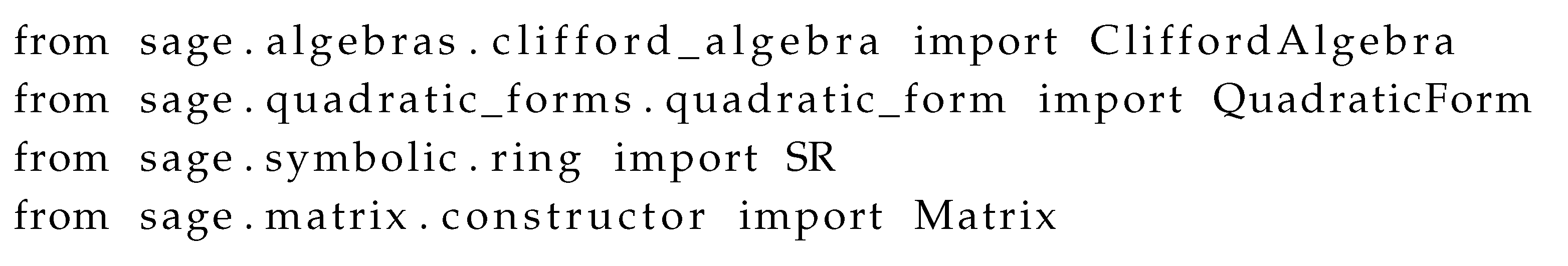
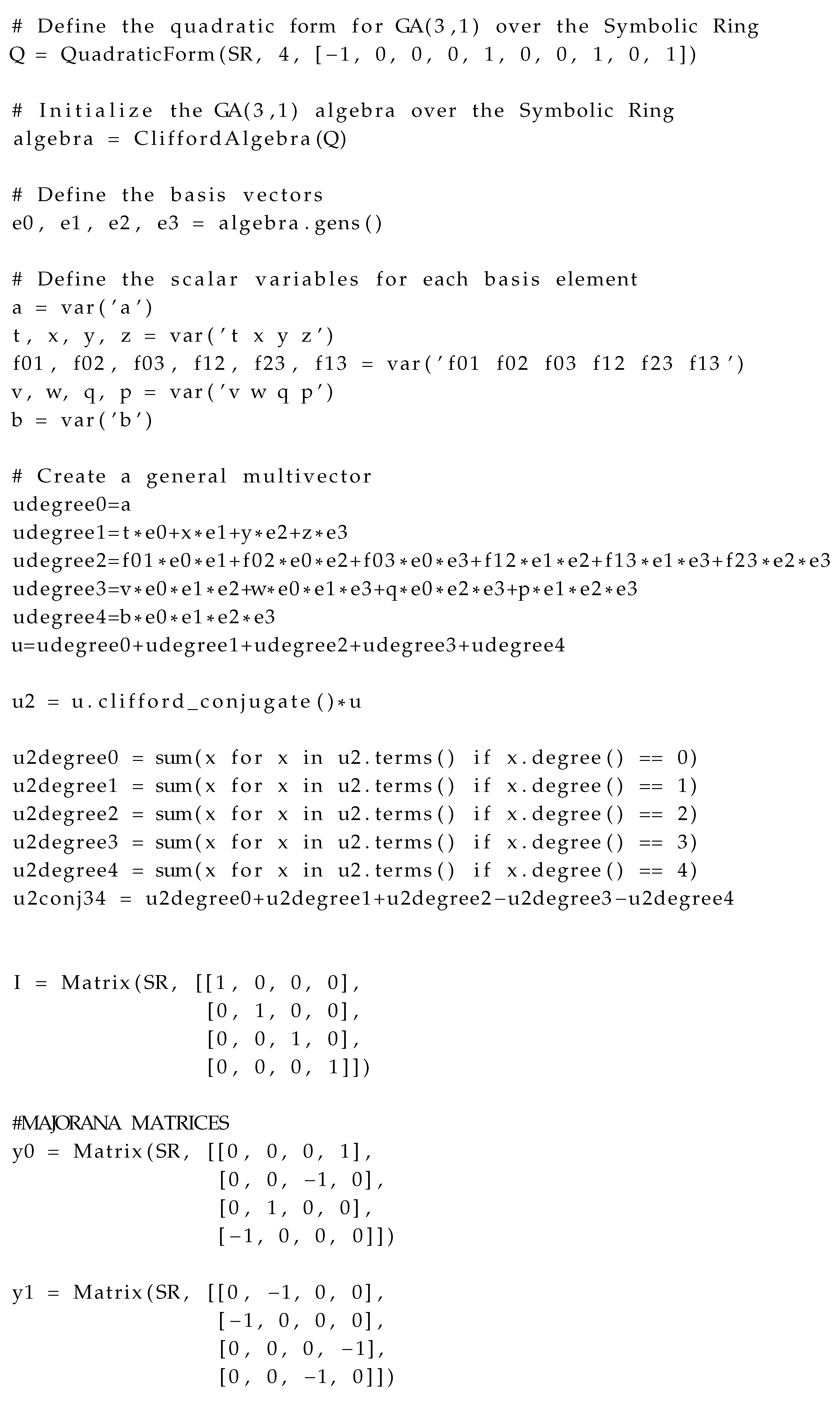
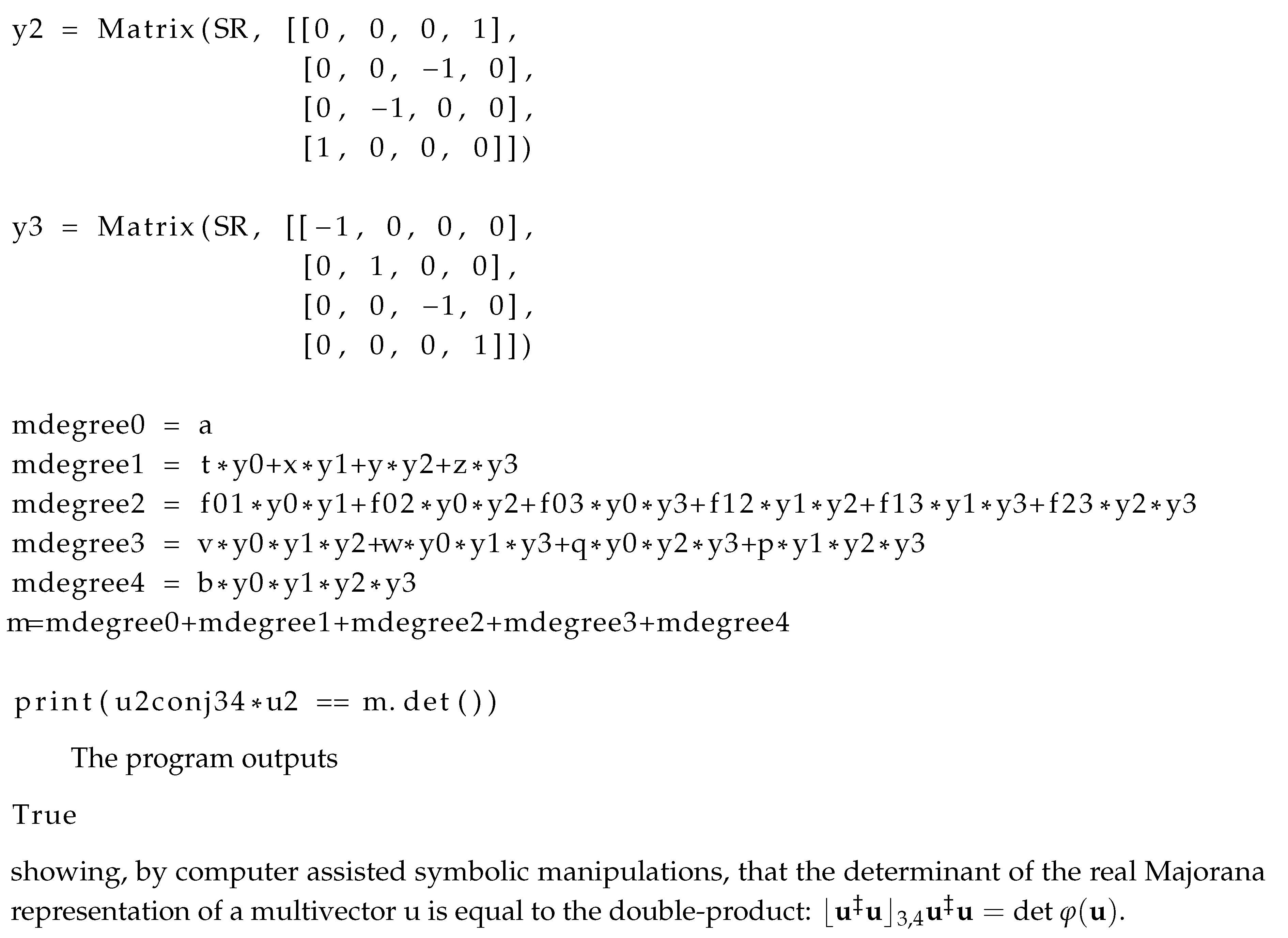
Appendix F SageMath program showing ⌊u ‡ u⌋ 3,4 u ‡ u=detϕ(u)
References
- Edwin T Jaynes. Information theory and statistical mechanics. Physical review, 106(4):620, 1957.
- Edwin T Jaynes. Information theory and statistical mechanics. ii. Physical review, 108(2):171, 1957.
- Paul Adrien Maurice Dirac. The principles of quantum mechanics. Number 27. Oxford university press, 1981.
- John Von Neumann. Mathematical foundations of quantum mechanics: New edition, volume 53. Princeton university press, 2018.
- David Hestenes. Spacetime physics with geometric algebra (page 6). American Journal of Physics, 71(7):691–714, 2003.
- Douglas Lundholm. Geometric (clifford) algebra and its applications. arXiv preprint math/0605280, 2006.
- Ali H Chamseddine and Alain Connes. The spectral action principle. Communications in Mathematical Physics, 186(3):731–750, 1997.
- A Acus and A Dargys. Inverse of multivector: Beyond p+ q= 5 threshold. arXiv preprint arXiv:1712.05204, 2017.
| 1 | The author suggests that observations, so defined, may constitute a broader conceptual category that could entail a richer landscape of effective theories beyond what experiments alone feasibly entail. Observations allow us to study parts of the universe whose complexity far exceeds our ability to precisely connect an initial preparation to a final measurement via unitary transformations in the laboratory. Accounting for this observed complexity suggests the development of effective theories across various domains, including biology, chemistry, complex systems theory, emergent phenomena, and cosmology. This extension of the optimization problem to observations, however, falls outside the scope of the current paper. |
| 2 | As statistical mechanics’ optimization problem does not reference an initial preparation, it could be argued, from these definitions, that it is based on observations and not on experiments. |
| 3 | This definition should not be taken as pejorative of observations. |
Disclaimer/Publisher’s Note: The statements, opinions and data contained in all publications are solely those of the individual author(s) and contributor(s) and not of MDPI and/or the editor(s). MDPI and/or the editor(s) disclaim responsibility for any injury to people or property resulting from any ideas, methods, instructions or products referred to in the content. |
© 2025 by the authors. Licensee MDPI, Basel, Switzerland. This article is an open access article distributed under the terms and conditions of the Creative Commons Attribution (CC BY) license (http://creativecommons.org/licenses/by/4.0/).
Copyright: This open access article is published under a Creative Commons CC BY 4.0 license, which permit the free download, distribution, and reuse, provided that the author and preprint are cited in any reuse.


