
Submitted:
14 April 2024
Posted:
15 April 2024
You are already at the latest version
Abstract
Tailings generated by mining account for the largest proportion of global waste from industrial activities. Copper is relatively uncommon world-wide, with low concentrations in sediments and waters, yet is very elevated around mining sites. On the Keweenaw Peninsula of Michigan, USA, jutting out into Lake Superior, 140 mines extracted native copper from the Portage Lake Volcanic Series, part of an intercontinental rift system. Between 1901-1932, two mills at Gay (Mohawk, Wolverine) sluiced 22.7 million metric tonnes (MMT) of copper-rich tailings (stamp sands) into Grand (Big) Traverse Bay. Here we examine: 1) 3D coastal elevation and reef bathymetry, 2) particle dispersal, 3) copper concentrations and leaching, plus 4) shoreline toxicity. About 10 MMT of tailings created a migrating coastal beach that stretches 7 km from the Gay pile to the Traverse River Seawall. Another 10 MMT are moving underwater on the coastal shelf, threatening Buffalo Reef, an important lake trout and whitefish breeding ground. Aerial photos, ALS (plane) LiDAR, and relatively inexpensive UAS (drone) surveys characterize shoreline structure and aid initial remediation. Because sands (natural beach quartz, stamp sand basalt) are silicates of similar density, particle dispersal is similar and challenging. However, stamp sand beaches contrast greatly with natural sand beaches in both physical profile and chemistry. Dispersing particles retain copper, and release toxic concentrations. Leaching is elevated by exposure to high DOC and low pH waters. Field experiments, shoreline seining, and benthic sampling confirm serious impacts on aquatic biota, supporting tailings removal.
Keywords:
Coastal Mine Tailings
; Keweenaw Peninsula
; LiDAR 3D Bathymetry
; UAS drone studies
; Particle Dispersal
; Specific Gravity
; Copper Concentrations
; Buffalo Reef
; Mohawkite Arsenic
; Toxicity
; Daphnia
1. Introduction
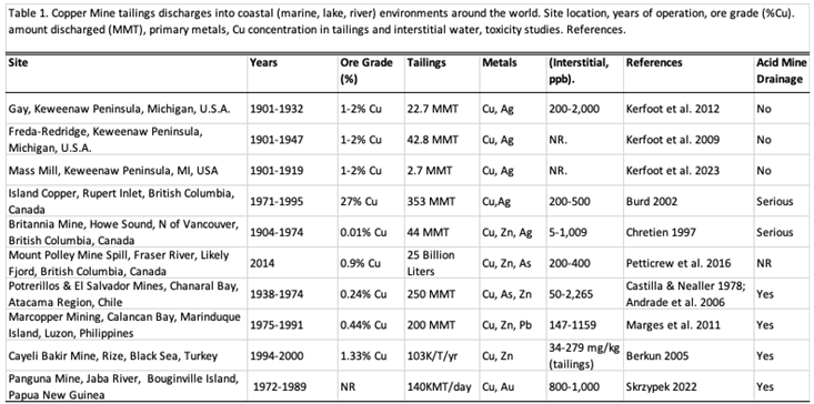
Worldwide, copper (Cu) is not an especially common element (26th most abundant), with dissolved Cu occurring naturally in relatively low concentrations [1,2,3]. Copper is enriched primarily near copper mining and smelting operations and in urbanized regions [2,4]. Aquatic environments are susceptible to Cu largely as receivers of tailings, urban and industrial wastewater, stormwater runoff, and industrial-era atmospheric deposition [1,2]. Tailings generated by mining and processing plants account for the largest proportion of global waste from industrial activities [5]. Despite lack of accurate data on the production of mine wastes, some estimates suggest as much as 20,000 to 25,000 million metric tonnes (MMT) of solid mine waste are produced annually around the world [6]. Table 1 lists several global copper mining sites that released tailings into coastal, lake, or river environments [7,8,9,10,11,12,13,14,15,16]. Mounting concern about discharge of mine tailings into coastal environments prompted the report (2012) “International Assessment of Marine and Riverine Disposal of Mine Tailings” by Vogt [17] for the UNEP Global Programme of Action for the Marine Environment. Vogt, among others [7,18], calls for more extensive studies of tailings dispersal, and a world-wide ban on coastal discharges. In countries with the highest copper production, Chile and Peru, lack of adequate management of tailings and mine closures remains a serious problem, as research has shown that contamination by mine tailings is significant for the health and environment of nearby communities [19]. Countries with the largest environmental footprint in copper production are the United States, China, and Canada [19,20]. In North America, coastal mining discharges remain prohibited in the Great Lakes since 1972, under the Clean Water Act, yet legacy sites are common, such as on the Keweenaw Peninsula. In 1990 [21], Chile also prohibited direct discharge of Cu tailings along their Pacific coast, yet allowed release of process waters with high dissolved concentrations (up to 2,000 µg/L).
 |
Issues here deal with consequences of legacy tailings dispersal and modern-day important impacts of dissolved copper on aquatic biota. Major lakes and reservoirs in the U.S. have dissolved concentrations of total Cu less than 10 µg/L (parts per billion, ppb; [22]). Concentrations in Canadian waters range from 1 to 8 µg/L Cu [23], whereas seawater concentrations rarely exceed 0.5-3 µg/L [24,25]. Locally, concentrations of dissolved Cu out in central Lake Superior are as low as 0.7 µg/L [26]. However, because of local natural ore deposits, background copper in Lake Superior sediments varies from 21-75 mg/kg (parts per million, ppm; [27]). Serious anthropogenic copper enrichments in Lake Superior nearshore sediments and waters are found primarily close to mining sites. Anthropogenic copper may exceed 200 µg/cm2 in offshore sediments around the Keweenaw Peninsula (Figure 1), plus 200-2,000 ug/L (ppb) dissolved copper in interstitial waters of tailings piles [8,28,29,30]. Globally, near mining, milling, and smelter sites, elevated total and dissolved copper are common-place in aquatic environments and are usually associated with toxic effects on biota (Table 1; [20,31,32,33,34,35]).
Copper from the Keweenaw Peninsula has a distinguished history. Indigenous people of Lake Superior (Chippewa/Ojibwe) traded copper from the Keweenaw Peninsula and Isle Royale extensively across Canada, the United States, and especially down through the Mississippi River before European settlement. Copper gathering and trading reach back at least to the Hopewill Culture, 2,000 years ago [9,36,37]. Copper gathering activity and pit excavations stretch back even further, 3,580-8,500 years ago on Isle Royale and the Keweenaw Peninsula [38,39], attributed to an “Old Copper Culture” that utilized copper-tipped spears.
Following the 1842 “Copper Treaty” with indigenous tribes, and extending until 1968, Boston and New York companies exploited the vast abundance of native copper and silver in the Keweenaw Peninsula [40,41]. The region became the second-largest producer of copper in the world during the late 1880’s to 1920’s, with 140 mines and 40 stamp mills [42,43,44]. Moreover, the industrial activity left a legacy of mine tailings, an estimated 600 million metric tonnes (MMT) of poor rock and processed tailings (stamp sands), deposited inland and along several coastlines of the Keweenaw Peninsula [7,8,45]. Yet the Keweenaw Peninsula and Isle Royale are unique, because most of the copper came from “native” copper, rather than from sulfide-rich deposits. Only at the extreme ends of the Peninsula, Bohemia Mountain Mine and Gratiot Lake deposits to the north, and the Nonesuch Shale deposits of the White Pine Mine to the south, are there copper sulfide-rich (chalcocite, Cu2S) ores. Most global locations exploit copper sulfide ores and must deal with acid mine drainage issues (Table 1 [46,47]). For example, a newly opened nickel and copper “massive sulfide” mine east of the Keweenaw Peninsula, in the Yellow Dog Sand Plains near Marquette, MI, helps satisfy recently increased demand for nickel and copper, yet includes acid mine drainage complications.
On the Keweenaw Peninsula, “stamp sands” are crushed basalt rock, released as a waste byproduct from “stamp” mills. The primary ore deposits are found in a series of billion-year-old lava flows, the Portage Lake Volcanic Series (Figure 1, dashed lines). Whereas original mining operations concentrated on removing large masses of copper, known as “barrel copper” [48], later operations shifted to extracting copper through crushing (“stamping”) large volumes of ore at mills. After crushing, particles were sorted by water-borne gravity separation, using jigs and tables [49] to form a concentrate (ca. 50% Cu) shipped off to smelters. The remaining crushed fractions, often around 98-99% of the processed mass, were sluiced out of the mill into rivers or along lake shorelines, creating beach deposits and bluffs along Keweenaw Peninsula shorelines (Figure 2).
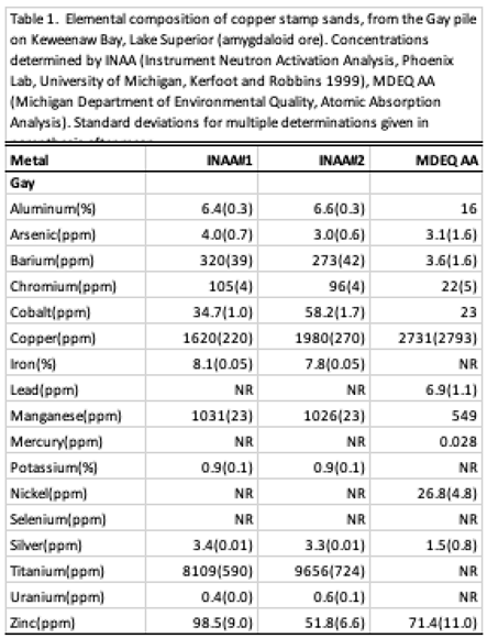
The early mill extraction was not very efficient, as around 10-20% of the ore’s copper was lost to tailings [42,49]. For example, at the Mohawk Mine site, average concentrations in ores (ore grade) averaged 1-2% Cu, whereas the Mohawk Mill discharged tailings averaging 0.28% copper, i.e., an estimated 6,810 metric tonnes of copper lost to tailings [50]. Historically, an ore containing 0.7-0.8% copper would be a mineable deposit on the Keweenaw Peninsula. In the later years of Torch Lake operations, Calumet-Hecla and Quincy Mines dredged and reprocessed early Cu-rich tailings piles (>1% Cu), adding 30% to revenues [49]. Because of such high Cu concentrations, stamp sands also became a serious contaminant source along beaches and in sediments, accompanied by an additional suite of metals, e.g., aluminum, arsenic, silver, chromium, cobalt, lead, manganese, mercury, nickel, and zinc (Table 2; [27,51], that occasionally flag state standards.
 |
On shorelines and along underwater coastal shelfs, there are mixtures of stamp sands and natural sands. The two major sand types at Grand (Big) Traverse Bay come from quite different sources (end members). The crushed Portage Lake Volcanics, the so-called “stamp sands”, are basalts (K, Fe, Mg plagioclase silicates; augite, and minor olivine), whereas eroding coastal bedrock (Jacobsville Sandstone) produces rounded quartz sands that make up the natural white beach sands [7]. Up close under natural sunlight (Figure 3a), individual stamp sand grains along the shoreline are largely brownish and gra y, yet sprinkled with scattered green, red, white, orange, yellow, and transparent sub-angular grain particles, the latter coming from so-called “gangue” minerals (e.g., calcite, epidote, chlorite, prehnite, pumpellyite, microcline, and K-feldspar; [52]) found in veins associated with the basalt. However, from a distance, the stamp sand beach deposits appear like dark gray beach sands (Figure 3b).
Stamp mills in the Keweenaw released an estimated 360 MMT of stamp sands along the Lake Superior coastline and inland lake shorelines and rivers [8,53]. For comparisons, the Mohawk and Wolverine Mills at Gay (Figure 4) sluiced 22.7 MMT of stamp sands onto the eastern shoreline, whereas four mills in the Freda and Redridge area of the west shoreline discharged around 45.5
MMT [8]. At Portage Lake in Houghton/Hancock (Figure 1), a total of eleven mills released around 10.1 MMT; whereas six mills at Torch Lake released 178.5 MMT [27,53,54]. Much of the stamp sand “coarse” fraction ended up as beach deposits or underwater sand bars, whereas the “slime clay” fraction (7-14% of total discharge [42,55]) dispersed much further. Slime clays drifted out to be deposited in deep water sediments of inland lakes (e.g., Portage and Torch Lakes) and spread off coastal shelves into deep-water canyons of Keweenaw Bay and Lake Superior (Figure 1; “halo”). Slime clays left excellent annual layers (“varves”) in Portage Lake sediment cores that can be easily dated [27,53]. In contrast, stamp sands tended to stay in place along low-energy shorelines of interior lakes, but moved kilometers along high-energy Lake Superior coastal shorelines by wave and current action (Figure 2; Gay, Freda-Redridge, Sand Point).
During and after deposition, the coastal tailings pile at Gay eroded as waves and currents moved stamp sands southwestward across the shoreline beach and coastal shelf (Figure 5a). Repeated LiDAR flights clarified 3D bathymetric details of shelf and reef environments and stamp sand movements. The reef is a major spawning ground for lake trout and whitefish, accounting for 32% of commercial fishing in Keweenaw Bay, and 22% of the catch along the southern Lake Superior shoreline [54,56]. Fortunately, migrating stamp sands initially encountered an ancient river bed (termed the “Trough”). Over the last century, the stamp sands filled the northern portions of the river bed and are now moving into cobble fields on the northeastern and western margins of Buffalo Reef [7,50,54]. From 2008-2016 LiDAR/MSS studies, the reef was estimated to be 25-35% covered by stamp sands [50,54,57]. Within the next ten years, if nothing is done, the Army Corps of Engineering hydrodynamic models predict increase in stamp sand cover to 60% [54,58].
The two LiDAR DEMs (digital elevation models, 2010, 2016) in Figure 5a,b also show that the coastline profiles of stamp sand beaches differ from those of natural sands. Natural sand beach depth profiles along the southwestern shoreline have a “cusp”-like series of structures and an underwater bar that contributes to a shallow wading zone, whereas stamp sands possess a higher, wider beach and a relatively sharp drop-off to greater depth along the shoreline edge. Stamp sand beaches continually enlarge down-drift to the Traverse River Seawall as stamp sands migrate southwestward from the Gay pile location [7,50]. Residents are afraid of youngsters slipping down the steep shoreline slope. Another issue with stamp sand movement is over-topping at the Traverse River Seawall.
Here we review 3D elevation/bathymetric features.
Here we review 3D elevation and bathymetric contours during particle dispersal, leaching of copper from drifting coastal tailings deposits, and impacts on aquatic organisms (toxicity). Previously, keying off albedo (darkness) differences between natural sand and stamp sand beaches, we used 3-band MSS data from 2009 NAIP imagery to plot the underwater incidence of stamp sands around Buffalo Reef [7,57]. However, that method did not allow calculation of stamp sand percentages within bay mixtures of stamp sand and natural sand. To address that question, we devised a simple bay-specific microscope method to quantify the percentage of stamp sand grains in mixed sediments (see Methods; also [29]).
Once the percentage of stamp sand is known at a site, an initial prediction of copper concentration (using the MDNR Gay pile value of 2860 ppm Cu as a standard) can be calculated. However, the calculation assumes random dispersal of copper among dispersed stamp sand particles, i.e., no differential density or particle size sorting. Two processes could alter relative Cu concentrations in dispersing stamp sands. First, coarse sand-sized particles with higher density (greater Cu) might remain closer to the source (Gay Pile). Recall that the mills used jigs to separate denser copper-rich particles from stamp sands as a routine part of processing. Wave action along the shoreline could perform similar sorting. Secondly, because the clay fraction at the original tailings pile contains higher Cu concentrations (greater surface to volume ratio; [27]), waves could also winnow out the fine slime-clay fractions from shoreline deposits, spreading these into reef crevices or out into deeper waters (contributing to the “halo” of Figure 1).
We show that stamp sands eroding from the Gay tailings pile cover the original natural white sand string beach west of the Coal Dock. Drone surveys confirm that the present-day stamp sand beach, especially near the Harbor Seawall, is wide and high. Surface stamp sand percentages are 80-90% from the original Gay Pile to the Traverse River Seawall. Shoreline percentages of stamp sand are highest between the Gay Pile and Coal Dock, but also in migrating underwater bars and in northern regions of the “Trough”. High percentages of stamp sand are also abundant around the Traverse Harbor location. Additional hi-resolution drone studies confirm that after bluff removal on the Gay tailings pile, shoreline erosion has increased.
To test assumptions of copper concentrations associated with percentages of stamp sands, we use our recent U.S. Army Corps of Engineers (Detroit Office) AEM Project (“Keweenaw Stamp Sands Geotechnical And Chemical Investigation”) survey data from 2019-2022. Direct assays document that, over the past century, there is substantial dispersal of stamp sand particles across the bay, yet slightly lower copper concentrations in stamp sands distant from the Gay Pile site. However, copper concentrations were initially so high in the Gay pile, that there remain serious environmental consequences along the entire shoreline from Gay to the Traverse River and in encroachments onto the reef. Leaching experiments done during 2019-2022 examine beach stamp sand release of fine particulate and dissolved copper into shoreline interstitial and beach pond waters. Stamp sand interstitial and pond waters contain elevated copper concentrations that are highly toxic to aquatic organisms. Our investigations and in-depth complementary USACE Vicksburg (ERDC-EL) findings show that high DOC and low pH waters, characteristic of nearby river, stream, and wetland (riparian) groundwater inputs, substantially accelerate leaching of Cu from shoreline tailing beach deposits. Overall, there is now a growing consensus that beach stamp sands constitute a serious shoreline contaminant threat to aquatic communities and should be removed.
2. Methods
CHARTS Coastal LiDAR (Light Detection And Ranging). LiDAR is an active remote sensing technique used over Grand (Big) Traverse Bay in the ALS (airborne laser scanning) version, where an airborne laser-ranging system acquires high-resolution elevation and bathymetric data [59]. “High-Resolution” here is relative, as ALS often has point density ranges of 0.9-17.4/m2, whereas UAS helicopter drone LiDAR point density may achieve values in the tens to hundreds. The ALS Compact Hydrographic Airborne Rapid Total Survey (CHARTS) and the Coastal Zone Mapping and Imaging LiDAR (CZMIL) systems are separate integrated airborne sensor suites used to survey coastal zones, in which bathymetric LiDAR data are collected with aircraft-mounted lasers. In coastal surveys, an aircraft travels over a water stretch at an altitude of 300–400 m and a speed of about 60 m s−1, pulsing two varying laser beams in a sweeping fashion toward the Earth through an opening in the plane’s fuselage: an infrared wavelength beam (1064 nm) that is reflected off the water surface and a narrow, blue-green wavelength beam (532 nm) that penetrates the water surface and is reflected off the underwater substrate surface (Figure 6a). The two-beam system produces a complex wave form (Figure 6b) that when processed, quantifies the time difference between the two signals (water surface return, bottom return) to derive detailed spatial measurements of bottom bathymetry in addition to ancillary light scattering data.
Laser energy is lost due to refraction, scattering, and absorption at the water surface and lake bottom, placing limits on depth penetration as the pulse travels through the water column. Corrections are incorporated for surface waves and water level fluctuations. In Grand (Big) Traverse Bay, we have used extensive LiDAR geophysical surveys (2008, 2010, 2011, 2013, 2016, 2019) to reveal underwater (bathymetric) and shoreline (elevation) features [29,50]. The resulting DEMs can be rotated from vertical to various horizontal angles to enhance 3D surfaces (29,57], or shading (Hillshade) added to again highlight 3D features. Surfaces from different dates can be compared to quantify erosion or deposition differences (Figure 5c; [29]). LiDAR surveys from 2008, 2010, 2016, and 2019 were used for this Project. In particular, USACE 2010 and 2016 LiDAR overflight data were preprocessed by the U.S. Army Corps of Engineers Joint Airborne Lidar Bathymetry Technical Center of Expertise (JALBTCX). Quality control and editing were done in GeoCue’s LP360, bulk datum transformations with NOAA’s VDatum, then products were generated using Applied Imagery Quick Terrain Modeler and ESRI ArcGIS (ArcMap and ArcGIS Pro).
The error associated with LiDAR DEMs (digital elevation/bathymetry models) is sensitive to several variables: mechanical collection (GPS coordinate system, scan altitude and speed, scan pattern, pulse-repetition rate, aircraft yaw and roll) and signal processing, weather, sea state, depth, water clarity, and wave-form clarity. Depth is important; for example, the horizontal and vertical accuracy of the CZMIL system has been described as 3.5 + 0.05 × d meters and [0.32 + (0.013 × d)2]1/2 m (Optech Manual), respectively, where d is the water depth. Details of resolution and accuracy in oceanic projects are discussed in several recent works [60,61,62,63]. With multiple instrument measurements, vertical LiDAR accuracy can be enhanced to 0.2 m in shallow coastal waters [64], and 0.22 (range 0.16–0.31 m) along terrestrial strips [65]. In particular, under low-flying, high-density scanning characteristics of coastal and Great Lakes shorelines, horizontal resolution is listed by JALBTCX as 0.5–1.0 m (0.7 m) along inland beach environments, with vertical accuracy of 15 cm (Optech Manual) [66]. Spatial resolution decreases to ca. 2 m in deeper waters (10–20 m). Underwater DEMs are usually delivered with tiled 3 m resolution.
Under ideal conditions in coastal waters, blue-green laser penetration allows detection of bottom structures down to approximately three times Secchi (visible light) depth. In Grand (Big) Traverse Bay studies, JALBTCX LiDAR repeatedly achieved around 20–23 m penetration [7]. The depth was somewhat less than the 40 m recorded from oceanic environments [67], yet adequate enough in Lake Superior to clearly characterize shallow coastal shelf regions and to highlight critical details of tailing migration (Figure 5a–c). Localized higher resolution results came from complementary drone, side-scan sonar, and ROV transects. Scattered Ponar and coring surveys provided ground-truth surface sediment characterization plus vertical studies that aided mass-balance calculations. Here we show how resolutions from aerial photography, ALS and drone LiDAR surveys complement each other and allow detailed bay elevation and bathymetric calculations, aiding construction of maps.
Unmanned Aircraft System (UAS) Studies: Traverse River Harbor, Berm Complex, And Gay Pile Erosion. A variety of remote sensing techniques are used for characterizing complicated small-scale geospatial features in large embayments. Options range from satellite imagery (Landsat-20m resolution, Sentinel 2-10m, PlanetScope-3m), use of Geographic Information Systems (GIS), Global Positioning Systems (GPS), Light Detection and Ranging (LiDAR) applications (satellite, plane, and drone), and tri-dimensional (3D) aerial scanning [68,69]. Here 3D aerial photography, high-resolution LiDAR pucks, were used on various drone (UAS) platforms. Both coastal erosion and deposition were modeled previously with conventional aerial plane photographs and ALS LiDAR overflights, plus sonar techniques [7,50,54,57,70,71], along with RGB drone images of the shoreline [29]. Underwater photography (ROV), conventional and side-scan sonar (IVER3), plus triple-beam sonar surveys have also aided interpretation of underwater surface details, Buffalo Reef, and shelf depths [7,50,54,72,73], but are not addressed here.
Recently, foreshore, backshore, dune, and underwater features were imaged with several low-cost Remotely Piloted Aircraft Systems (RPAS; Figure 7) including MTRI’s (Michigan Tech Research Institute’s) relatively large Bergen Hexacopter and Quad-8, plus several medium and smaller quadcopters, including a Mariner 2 Splash Waterproof, which carried camera packages or LiDAR pucks (Velodyne VLP-16). Systems are all hi-resolution, providing point densities of hundreds per meter, and resolutions between millimeters to a centimeter, depending on copter height and respective packages [Figure 7].
In the bay, the RPAS all met the US Federal Aviation Administration’s definition of a small UAS (<25 kg). The largest system was a hexacopter (six rotor) system (Figure 7) manufactured by Bergen RC Helicopters of Vandalia, Michigan. The device has several important attributes, including being remote control, capable of at least 15-20 min of flight time, having on-board position data from a GPS, a return to home default capability if connections are lost, ability to fly a payload of up to 5 kg, a tiltable sensor platform, and a reasonable cost (US $4,500-$6,200). In addition, MTRI developed a lightweight portable radiometer (LPR) system that enabled spectroscopy at a lower cost and lighter weight than traditional handheld systems, such as the ASD FieldSpec 3 [74]. The LPR is compact and light enough to be flown onboard a UAS that is capable of lifting at least 1 kg and is housed in a plastic box that can be attached to a typical UAS payload platform. The device is capable of deploying multispectral cameras up to the size of a Nikon D810 full-frame camera, plus multispectral cameras [a Canon point-and-shoot 16 mp camera for natural color (RGB) data collection, with overlay capability of producing 3D images; a second Canon point-and-shoot camera modified to be sensitive only to the near-infrared range of ca. 830 to 1100 nm]. A Velodyne LiDAR Puck can also be fitted on the platform. The Bergen hexacopter’s tiltable sensor platform enabled the LPR system to face forward during takeoff, then be repositioned to nadir for spectral data surveys.
The Bergen Quad-8 was a reliable system for deploying a variety of air-born sensor systems [75,76,77]. During initial testing for aquatic applications, we found the minimal flying height (ca. 10m) at which downwash from the Bergen hexacopter does not disturb the water surface, to an extent that it interferes with spectra and imagery. The minimal flying altitude of ca. 10 m was used for collecting spectral data, whereas a height of ca. 25 m was used for natural color image collection. Smaller DJI Phantom 2 Vision, Phantom 3 Advanced, and Mavic Pro Quadcopter UAS were also used to provide rapid, lower resolution imagery (12 mp), yet sufficient to provide orthophoto mosaic basemaps of study areas, at very reasonable costs ($1600; micro down to $500). In 2021, a DJI Mavic 2 Enterprise Advanced (M2EA) drone platform, had an integrated thermal (FLIR Vue Pro) and optical camera (Nikon D810; 20-megapixel camera). The UAS-collected images are processed through Structure From Motion (Sfm) photogrammetric software packages such as Agisoft Metashape to create Digital Elevation Models (DEMs), Hillshade Imagery, GeoTIFFs and R-JPG formats of data. ArcGIS Desktop and ArcGIS Pro aided presentations. In UAS LiDAR, imaging point density was limited to around 29.4 points/ft2 (316.3 points/m2), by payload capacity, yet allowing 100-fold more resolution than ALS LiDAR surveys.
Specific Gravity Studies. Specific gravity is the density of a substance relative to water, where one cm3 of water under standard conditions is one gram with a specific gravity of 1.00. We investigated specific gravity as a means to determine the percentage of stamp sands in mixtures with natural sands. In Grand (Big) Traverse Bay, natural beaches are primarily quartz grains, derived from wave-based erosion of Jacobsville Sandstone bedrock (Figure 5a,b), which covers the eastern half of the Keweenaw Peninsula and also outcrops on Buffalo Reef and along the bay shoreline and shallows. Stamp sands are basalt, also a silicate, which in ores host an assortment of minerals and metals (e.g., Al, Fe, Mg, Mn, Cu). The mean density of pure quartz is around 2.65 g/cm3, whereas that of basalt is around 2.9 g/cm3, a difference of only 9.4% [78,79]. For comparison, the specific gravity of pure copper is much heavier, around 8.95, although amygdaloid ores generally contain only 1-2% copper [42]. The Army Corps once attempted to use specific gravity to estimate %SS in a single mixed sediment sample from lower Traverse Bay, so we investigated this approach further in Grand (Big) Traverse Bay with multiple comparative measurements in the laboratory and field.
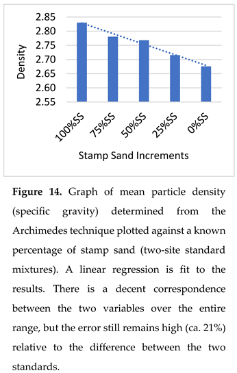
Applying the classic Archimedes technique, masses of 100% beach stamp sands (Gay Tailings Pile) and 100% natural quartz sands (Schoolcraft Beach, lower bay) were selected as standards. Plastic drums of sands were collected from the two sites. The drums were stirred to mix contents, then subsamples weighed. A 2000mL glass graduated cylinder was filled with 1000mL of distilled water under room temperature (20oC). After repeated mixing, ten masses of 200-400 grams were dried and sonicated to separate grains. The weighed sediments were dropped carefully into the cylinder and the volume displacement of water recorded. Once the weight and volume were known, the mean specific gravity in g/cm3 for the sample was calculated, plus corresponding measurement errors. We also mixed the 100% stamp sand standard (Gay Pile) with increasing amounts of the 100% natural quartz sand (Schoolcraft) standard to form a known series (100%, 75%, 50%, 25%, 0% stamp sand mixtures by weight). At each mixture, five subsamples were placed in the 2000 mL graduated cylinder for measurement of volume and calculation of specific gravity. A regression line was fit to the entire range of measurements. To assess accuracy and precision of the procedure, measurement error was compared with the specific gravity difference between the two standards. The specific gravity technique had around a 20-30% relative error (see Results). During the procedure, concerns about relative error and the time of effort prompted us to adopt an alternative approach, the “particle counting technique”.
Microscope Particle Grain Counting Technique. As mentioned earlier, the two major sand types in the bay come from different sources (end members). The crushed Portage Lake Volcanics, the so-called “stamp sands”, are basalts (K, Fe, Mg plagioclase silicates; augite, and minor olivine) with angular crushed edges, whereas the coastal bedrock (Jacobsville Sandstone) produces rounded quartz sands that make up the white beach sands (Figure 8a). The two types are silicates with similar specific gravities, and particle size distributions are often very similar (Figure 8b). We emphasize that the particle counting technique is appropriate only for sites (like Grand/Big Traverse Bay) where the two grain sources are very different and the majority of particles are sand-sized.
In Traverse Bay, under the microscope (Olympus LMS225R, 40-80X), particle grains from beaches and underwater coastal shelf Ponar samples could be separated into crushed opaque (dark) basalt versus rounded, transparent quartz grain components (Figure 8a), allowing calculation of %SS particles in sand mixtures. Percentage stamp sand values were based on means of randomly selected subsamples, with 3-4 replicate counts, around 300 total grains in each sub-count. Standard deviations and errors were calculated for individual samples and means used to calculate confidence intervals for typical counts (Figure 8c; Supplemental Tables S1 and S2).
Technically, mixed grain counts follow a binomial distribution, where there is an inverse relationship between the coefficient of variation (CV = mean/SD) and the mean %SS (Figure 8c). That is, from Figure 8c, if the mean %SS is high (>50%), the Coefficient of Variation (CV = mean/SD) is relatively low (3.1%, N=12 samples), but if it is <10%, the value could be much higher (mean = 25.3%, N= 30 samples).
However, in natural white sand beaches, there may be scattered black sand grains that are inadvertently scored as stamp sands, if only transmitted light is used in the microscope assay technique. Natural magnetite, ilmenite, garnet and manganese sands [80,81,82] are present, but relatively scarce, in Jacobsville Sandstone sand beaches and underwater bay sand sediments. Specific gravity and density may also be used for particle separation, as magnetite (5.2 g/cm3), ilmenite (4.5-5.0 g/cm3), and garnet (3.4-4.3 g/cm3) are much heavier than stamp sands (2.8-2.9 g/cm3). Under the microscope, reflected color, and size can also be used to distinguish magnetite sand grains (characteristic gray, glossy metallic color) from stamp sand basalt particles (low to no transmission of light; dark brown, dull gray, or greenish; often with inclusions). Magnetic attraction will also confirm magnetite abundance. Magnetite granule corrections are important for beach samples, but grains are rather low in Ponar samples across Traverse Bay shelf regions (averaging only 1.8% of grain counts). See Supplemental Table S4, which provides examples of magnetite “black sand” counts and corrections for percentage stamp sand determinations (beach and shelf samples).
Particle Sizes & Sieving. Grain sizes were also measured in selected samples under the microscope, distinguishing between stamp sand and quartz grains (Figure 7b). Otherwise, entire samples were sieved for various particle size classes. Wildco Stainless Steel Sieves (5 Mesh, 4000 µm; 10 Mesh, 2000 µm; 35 Mesh, 500 µm; 60 Mesh, 250 µm; 120 Mesh, 125 µm) were used on a Cenco-Meinzer Sieve Shaker Table (Central Scientific) or, after 2022 sampling, a Gilson 8-inch Sieve Shaker w/ Mechanical Timer (115V, 60Hz) model SS-15. Mean particle sizes from the Ponar samples were plotted across Grand Traverse Bay (see Results). See Supplemental Table S3 for latitude-longitude locations and particle size distributions in the full set.
Predicting Cu Concentrations From Stamp Sand Percentages. Extensive MDNR sampling on the Gay pile [83] gave a mean concentration of 0.2863 % Cu, or 2,863 ppm. We adapted this value as a standard. The standard provided a first estimate for Cu concentrations in mixed sand particle samples across the bay, assuming sorting was random and wave action transported similar sizes of both particle types across different sites. Copper concentration could be determined by simply multiplying percentage stamp sand by the MDNR Pile value [29]. For example, a 50% SS mixture would produce a predicted Cu solid phase concentration of 1415 ppm Cu, a 25% SS mixture 716 ppm, and a 10% mixture 286 ppm. Notice, the original concentration of Cu at the Gay pile is high, relative to expected Cu toxicity. Even a 10%-20% SS mixture would exceed EPA and Michigan PEL levels (probable effects levels; range from 36 to 390 ppm; [84,85]). However, as mentioned earlier, two pressing issues argue against random Cu dispersal: 1) there may be differential sorting by particle density or size, i.e., particles with Cu might be heavier and settle closer to the pile source; and 2) the fine fraction (slime clay), that has higher Cu concentrations (0.4%), might be winnowed out of redeposited beach sands and dispersed further out into the lake, contributing to the “halo” (Figure 1). Both actions would reduce Cu concentrations in beach sand/stamp sand mixtures as they disperse from the Gay source pile. Hence the importance of directly determining copper concentrations in samples as a check.
Direct Cu Concentration Comparisons (Selected Ponar Samples, AEM Project Determinations). Initially, to check our %SS predicted Cu concentrations against directly observed Cu concentrations, we determined Cu concentrations on several Ponar and beach samples, then constructed a “calibration curve” showing predicted Cu concentration against observed Cu concentration, using up to 40 samples [29,50]. For direct Cu determinations, beach and Ponar sediments were digested at MTU in a microwave (CEM MDS-2100) using EPA method 3051A. Solutions were shipped to White Water Associates Laboratory for final analysis. Copper was measured using a Perkin-Elmer model 3100 spectrophotometer. Digestion efficiencies were verified using NIST standard reference material Buffalo River Sediments (SRM 2704), and instrument calibration was checked using the Plasma-Pure standard from Leeman Labs, Inc. Digestion efficiencies averaged 104%, and the calibration standard was, on average, measured as 101% of the certified value. There was initially a good correlation between %SS predicted Cu concentration and directly measured Cu concentrations, R2 = 0.911 [50]; and R2 = 0.868 [29]. However, regression slopes and intercepts suggested slightly lower than predicted values.
As a major independent check on the microscope %SS method and its correspondence to Cu concentrations across bay sediments, we collaborated in an extensive Army Corps AEM Project (2019-2022). The Project directly compared our %SS predictions with direct Cu analysis of beach stamp sand and underwater shelf sediments across Grand (Big) Traverse Bay, using a combination of Ponar and coring techniques. Percentage stamp sands (% SS) were determined in our MTU laboratory using the microscope particle counting technique, whereas the corresponding Cu analysis was run at Trace Analytical Laboratories, Muskegon, MI.
The full AEM set included Ponar and core samples from three different locations: 1) deep water (DW; 7 samples; not really appropriate for the microscope technique; but retrieved after sand-sized sieving), 2) over water (OW; 52 coastal shelf samples, sand mixtures), and 3) on land (OL, beach sands; 104 sand samples). Again, normally the technique would not be used on deep-water samples because they are dominated by silt and clay-sized particles (62.5µm - 0.98µm; [86]), so some grain sieving was necessary to retrieve sand-size particles. The “Over water” samples were from the shelf region, generally dominated by medium to fine sand-sized particles (0.5mm - 125µm; Supplemental Table S3). The “On Land” sites were all beach deposits with medium sands to fine gravel (0.25mm-8mm). The combined 164 samples were dominated by beach samples (see Appendix Table A.1), largely because beach cores were sliced into sections, moving from upper stamp sands into lower quartz sand (original beach) deposits southwest of the Ore Dock, the start of the natural quartz beach deposits.
As mentioned earlier, copper concentrations were run independently at Trace Analytical Laboratories, Muskegon, MI. Results from the AEM analyses are plotted in the Results regression section. An issue with the tabulated data from AEM Cu determinations was great variability in Cu concentrations beyond 50% Stamp Sand mixtures, especially in the beach core studies. Some of the great scatter was due to low standards (AEM Report). To better handle the variation, we considered the data sets as independent runs and dealt with the scatter by a variety of conventional statistical methods. Due to heteroskedasticity, fitting a regression line to the entire original set was not appropriate, since the variance around regression increased with %SS and Cu Concentration plots (especially >50% SS), leading to inappropriate regression application. These heteroskedastic effects could be reduced by a variety of statistical methods: 1) log transforming the data, 2) plotting grand mean values of Cu concentrations at intervals of % SS, or 3) looking at only a portion of the set (e.g., the lower end, 0-50% SS) where there was less heteroskedasticity. We utilized options 2 and 3. In addition, a table was constructed which listed the previous “calibration curve” regression [29], along with the three various AEM regression equation intercepts. In that table, the 100% SS regression intercept values could also be cross-compared against the mean Gay Pile standard value (i.e., the MDNR 0.2863 ppm value).
Copper Leaching Studies: Laboratory & Field. At MTU, preliminary experiments looked at leaching of Cu from agitated coastal stamp sand particles, using various water types. Waters were chosen to: 1) represent shallow clear coastal waters from Lake Superior with low TOC/DOC, and 2) tannin-stained waters from the river and wetland swales that have relatively high TOC/DOC and low pH. Tannin-stained and lower pH waters were selected because they were characteristic of local stream and river waters (Traverse River, Tobacco River, and the Coal Dock stream), and occur in neighborhood forest and wetlands (Nippising Beach Complex). Several gallons of water (5-10) were collected at five different field sites. Subsamples were placed in 140mL polyethylene bottles. In the agitation experiment, for each water type, flasks were prepared that contained 5g of 100% stamp sand (Gay Tailings Pile) and 25mL of water (i.e., 1:5 solid to liquid ratio). The vials were shaken and stirred periodically on a shaker table for an interval of one week. Thus the agitation was a single, prolonged leaching exposure. At the end, samples were run for both total suspended copper and separately for filtered (0.45 um; dissolved) copper. Nitric acid (1%) was added to each dissolved sample and the initial samples were cold-stored (4°C) until sent for metals analysis at the MTU School of Forestry Laboratory for Environmental Analysis of Forests (LEAF Lab). A Perkin Elmer Optima 7000DV ICP-OES was used separately for determining total and dissolved metal concentrations (for Cu, Al, Fe). The filter paper used for dissolved Cu concentrations was Pall Corporation Supor 0.45µm 90mm disk. The five different water sources were also analyzed for pH and TOC/DOC. Total organic carbon (TOC) and total nitrogen (TN) were determined using a Shimadzu TOC-LCPH analyzer with TNM-L. A ~25mL subsample of water had its pH measured using Fisher Scientific Accumet AE150. The TN analysis is not discussed here, but deals with productivity.
In 2019 and 2022, to check copper leaching at field locations, we collected water samples from various beach stamp sand ponds just southwest of the Gay pile (Pond Field, Figure 5a,b). These water samples also had a total metals analysis done on them for Cu and Al, again at the LEAF Lab. The 2022 stamp sand pond waters were not identical to the 2019 pond waters due to construction of the “Berm Complex” and subsequent neighborhood mixing of waters. However, sampling several ponds (15 samples) provided a range and mean of total Cu concentrations typically confronted by aquatic organisms on stamp sand beaches.
In addition to our preliminary measurements, the Army Corps, as part of the Buffalo Reef Project, sampled stamp sands, pond and interstitial waters from the Gay pile and “Berm Complex”. Samples were sent to various ERDC-EL facilities in Vicksburg, MS, for chemical characterization and more extensive leaching experiments with multiple and variable water rinses. The results of those detailed beneficial use application and physical and chemical investigations are found in an internal Report (Schroeder, P.; Ruiz, C. Stamp Sands Physical and Chemical Screening Evaluations for Beneficial Use Applications; Environmental Laboratory U.S. Army Engineer Research and Development Center: Vicksburg, MS, USA, 2021). In our leaching section, we discuss both the ERDC stamp sand chemical characterization and especially the leaching experiments. These valuable studies were complementary, conducted at the same time as the AEM Project. However, Vicksburg’s suite of chemical tests for stamp sands and contaminant pathways included a much broader range: pH, TOC, copper, arsenic, aluminum, antimony, beryllium, cadmium, chromium, cobalt, lead, lithium, manganese, mercury, nickel, selenium, strontium, thallium, and zinc.
Field (Stamp Sand Pond) And Laboratory Toxicity Experiments. In 2019, to check for toxicity of waters on invertebrate organisms, a Daphnia survivorship and fecundity experiment was run in the stamp sand ponds. A corresponding “Control” was placed at the Great Lakes Research Center dock in Portage Lake water. The Gay and Control field tests used the same suspended vial arrangement (Figure 9). The vial arrangement was also identical to a later lab test used to check acute LD50 values for Daphnia. Water exchange rates in the field mesh-covered vials were measured earlier in 1990′s pond placements, using methylene blue dye [87,88]. The Daphnia used in the stamp sand pond experiments were native species (Daphnia pulex) collected from nearby forest ponds [88]. At each pond, a rack with forty 40mL vials covered with 100µm mesh (Figure 9), and initially filled with filtered Portage Lake water, were set on a shallow pond sediment bottom. One adult Daphnia was placed in each vial. Every two to three days, the Daphnia vials were retrieved, survivorship and fecundity scored. The experiments lasted for fourteen days or until survivorship reached zero.
In the laboratory, D. pulex were raised in filtered (Supor®-450 0.45µm) water from Portage Lake. Laboratory feeding was Carolina Supply Daphnia food. Cultivating procedures followed USEPA 2002 guidelines [87]. Twenty years earlier (1990’s), laboratory LD50 tests were also conducted on native D. pulex [88,89]. Since nearly identical procedures were used, our recent results could be cross-compared with earlier in situ survivorship and fecundity, plus lab LD50 results, to see if pond conditions had changed.
In addition, expanding comparisons, a live Daphnia magna stock was ordered from Carolina™. The Daphnia magna were placed in 40 mL vials (the same set-up used in the pond experiments) filled with 40mL of Bete Grise Lake Superior water and stock Cu solutions in a dilution sequence. The stock solutions consisted of 1L of Bete Grise water with 1mg of dissolved Cu, creating a potential stock solution of 1,000 ppb Cu, which was diluted to test concentrations. The sequence used ten replicant vials at each Cu concentrations of 1,000 ppb, 500 ppb, 250 ppb, 100 ppb, 50 ppb, 25 ppb, 10 ppb, 5ppb, and 0 ppb. Copper concentrations were made by dissolving cupric sulfate (CuSO4 5H2O) salt in filtered Bete Grise water. As a check, a subsample of the stock solution was sent to the LEAF Lab to check expected Cu concentrations. As a consequence, after direct LEAF Lab measurements, concentrations were slightly adjusted. The survival of adults was recorded at 24hrs, 48hrs, and 72hrs for each vial at each Cu concentration value. A probit test was done for 24hr data to calculate the estimated LD50 value. The LD50 value was then compared with published literature values for D. magna and other Daphnia species [90,91], including our earlier 1990′s estimates for neighborhood D. pulex.
3. Results
UAS Studies: Stamp Sand Accumulation Downdrift, Seawall Over-topping, Initial Dredging & Remediation (2017-2022), Gay Bluff Removal And Accelerated Shoreline Erosion.
ALS LiDAR (Figure 5a,b) and UAS drone studies (Figure 10a,b) confirm that stamp sand beaches have different bathymetric profiles compared to surfaces off natural quartz sand beaches. UAS drone surveys have high resolution, millimeters to a centimeter [77]. A UAS Orthomosaic and Digital Elevation Model (Figure 10b) emphasizes that stamp sand dunes are growing higher as more sand arrives at the Traverse River Harbor site. Stamp Sand beach edges plunge at steep angles (30-45o). Water depths are greater along the stamp sand beach shoreline (Figure 10b, surf zone).
Increased depths allow waves to strike with stronger force along the stamp sand beach edge, tossing stamp sand up over the edge, helping increase heights. In contrast, natural quartz beaches have a more gradual transition in water depth offshore (Figure 5a,b and Figure 8a). Moreover, the surfzone of natural quartz beaches has a complex cusp structure inshore and a bar structure slightly offshore (Figure 5a,b). Waves tend to break further out on the sand bar, creating less impact along the natural beach front. During severe winter storms (e.g., October 17, 2017), video photos show higher waves breaking along the stamp sand beach, throwing stamp sand onto the dune pile and across the Seawall (over-topping). A series of depth profiles from drone surveys (Figure 10b) document the greater elevation of accumulating stamp sand near the beach edge and Traverse River Seawall. Based on experience, local resident’s have modified their attitudes. Gone are notions that stamp sand beaches “protect” landowners during storms. Rather, the stamp sand beaches are now seen to aggravate circumstances, allowing increased wave action to lift more stamp sand up across cabin lots. Moreover, the stamp sand beach front has become more dangerous, with a steeper drop and deeper water immediately offshore, characteristics not conducive to beach recreation.
Aerial photography and LiDAR studies by others elsewhere along natural beaches has also revealed repetitive cuspate structures associated with exiting surfzone currents [92,93,94]. Wave hydrodynamics and local beach currents and micro-structures modify both nearshore sediment transport and wave breaking. The use of conventional (ALS) and high-res UAS LiDAR imaging has confirmed beach change related to nearshore microstructure [7,50,94]. In Grand (Big) Traverse Bay, conventional and UAS elevational measurements aided Vicksburg’s hydrodynamic modeling efforts [58], as larger waves provided a mechanism that makes stamp sands migrate faster along the shoreline and move further inland than originally anticipated. Since 2020, seasonal stamp sand removal at the Seawall and Harbor channel expanded as part of Army Corps Stage I (2017-2022) remediation, discussed below (Figure 11a-Army Corps Maps].
A series of stamp sand rearrangements and removals were conducted at the Traverse River Harbor and at the Pond Region to the north. The dredged material came from two sites: 1) the Traverse River Harbor [removing “over-topping” stamp sands from the “blue” region of the harbor (Figure 11a)]; plus removing stamp sand from a rectangular “orange” “ region that received yearly migrating amounts (later greatly enlarged to a 300 m stretch) and 2) from the “Trough” [Figure 11a]. The Trough “red-rectangle” region removal aimed at reducing migration of stamp sand out of the Trough into cobble beds on Buffalo Reef. In addition, at the Gay pile site, the original 10-20m bluffs (Figure 2b,c) were removed down to nearly water level (2017-2021) with the material pushed southward or added to the shoreline of the Pond Site. At the “Pond Site”, slightly to the southwest of the original pile, the “Berm Complex” was constructed in 2020 to receive dredged material (Figure 11b). In addition, at the Gay pile site, the original 10-20m bluffs (Figure 2b,c) were removed down to nearly water level (2017-2021) with the material pushed southward or added to the shoreline of the Pond Site (Figure 12).
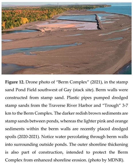 |
Over-topping stamp sands from the Traverse River, and also “Trough” dredged material were transported 3-7 km to the “Berm Complex” by 2-foot plastic pipe (Figure 11b). The “Berm Complex” walls were made of stamp sand, and so were relatively porous. When dredged spoils were delivered by pipe, contaminated waters seeped through the porous walls into surrounding ponds (Figure 12). Moreover, during transport, the grains were unintentionally severely mixed and tumbled, similar to our “leaching” experiment. Unfortunately, transported stamp sand also abraded surfaces and did damage to both pumps and plastic pipes. Because water from the Traverse River was enriched in natural humic substances and had a lower pH, there was genuine concern about increased Cu leaching during transport.
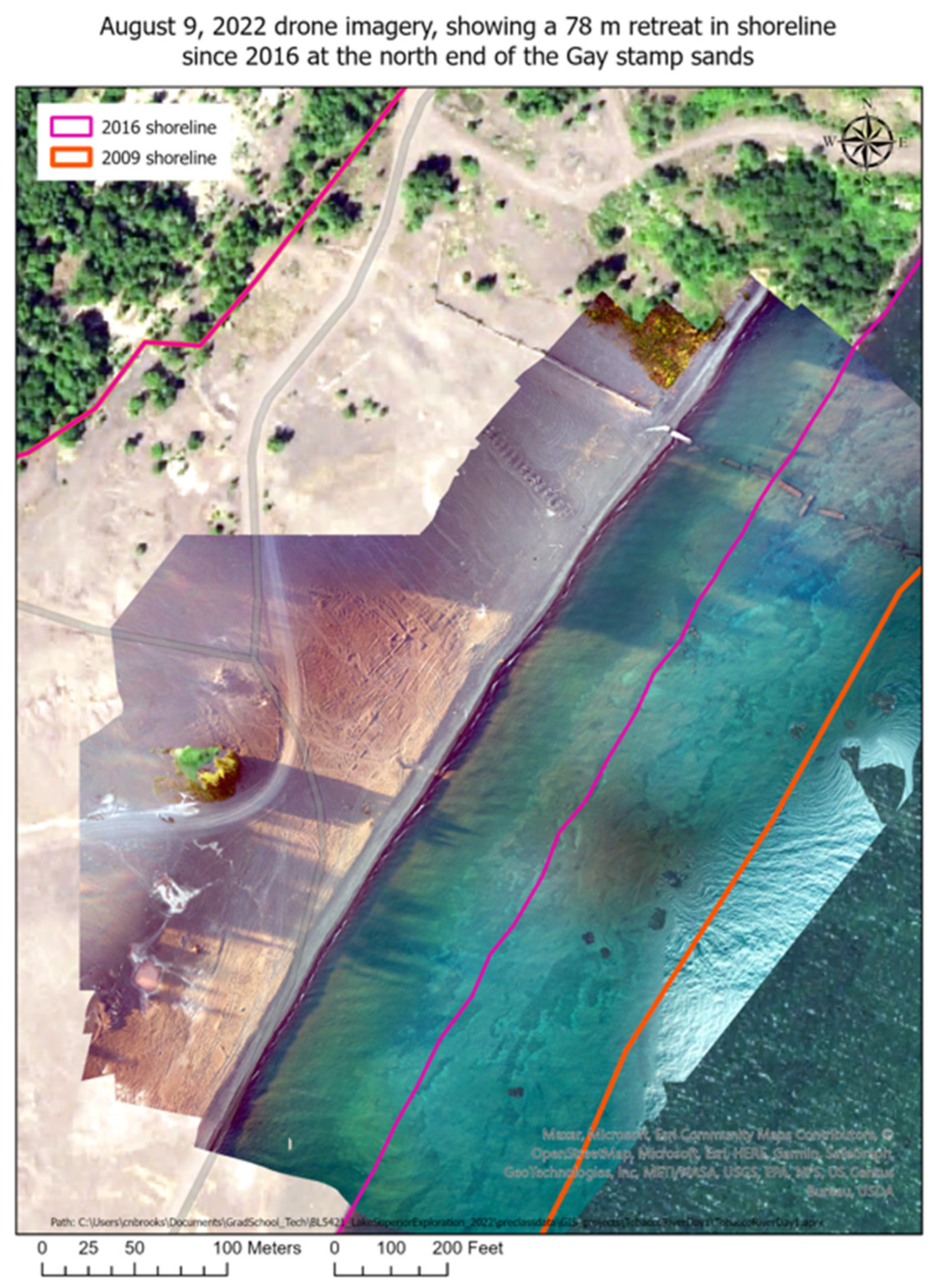
Subsequently, bluff removal increased shoreline erosion along the Gay pile region (Figure 13). Note high resolution details, such as the position of orginal wooden launder support beams (Figure 2c) after bluff removal and the collapsing concrete launder (also seen in background of Figure 2b,c). Recovery is underway, as trees are now invading what is left of the Gay Pile surface, whereas benthic organisms and fish are returning to the cleared bedrock stretches of the coastal shelf. Whereas aerial photos at the pile site documented an almost constant recession rate of ca. 7.9m (26′)/yr for nearly 80 years (1938-2008; [7,57]), the recession rate at the shoreline pile site has now increased to between 10.7 m/yr-13 m/yr.
Figure 13.
UAS high resolution drone elevation and bathymetry surveys (Aug. 9, 2022) of shoreline retreat at the original Gay pile location. Overlays along the beach edge show shorelines in 2009, 2016, and 2022. There has been a 78 m retreat over 6 years (2016-2022); hence a recent 13 m/yr retreat. The previous, nearly constant, long-term retreat rate prior to 2009 averaged 7.9 m/yr (25.3′) [7,57]. The original Jacobsville Sandstone shoreline, before stamp sands were discharged, is indicated by the red border in the far left upper region. In these hi-resolution drone surveys, remnants of both the wooden and broken concrete launders (Figure 2) can be seen in the middle region. Recovery is underway, as benthic organisms and fish are returning to cleared underwater stretches of the bedrock shelf, whereas scattered trees (many birch) are beginning to colonize what is left of the orginal Gay Pile surface (<10% original mass).
Dispersal Of Stamp Sands: Use Of Specific Gravity. A major challenge across the bay is determining the percentage of stamp sands in beach and underwater shelf environments, because natural sand mixes with stamp sand. Density differences between crushed basalt and quartz grains are only modest, as both are silicates (see Methods). In the lab, a “standard” sample of stamp sands from the Gay Tailings Pile had a mean density of 2.88 g/cm3(SD= 0.109, SE=0.034; N= 10) whereas one from the “natural quartz” Schoolcraft Beach site had a mean density of 2.55 g/cm3 (SD= 0.124; SE= 0.039; N=10). The mean difference between the two sites (N = 10 subsamples each) was 0.33 g/cm3 or 12.2% of mass. The difference was a bit larger than the literature rock type standards (see Methods), but still relatively minor.
Separately, for individual measurements, when we divide the standard deviations by the mean difference (CV = SD/mean) of the two standards, to get a coefficient of variation for measurement error, the CV varies around 20%. As mentioned in the Methods, the relatively low precision of this technique favored the microscope counting technique. Independent specific gravity measurements of stamp sand beach deposits from three coastal sites measured by the Army Corps (Gay Pile, Coal Dock, Traverse River Seawall) were 2.79, 2.83, and 2.7 g/cm3, respectively [95], close to our stamp sand standard. Site similarities largely result from the high percentages of stamp sand along the entire Gay to Harbor beach stretch.
We also mixed known percentages from the two sites (Gay & Schoolcraft beach samples) to form a set of samples with known percentages of stamp sand and natural quartz sand, then used the graduated cylinder technique to check mean specific gravity (Figure 14). The measurements show the expected declining density, yet the standard deviations around individual estimates (N = 5; 0.016-0.050, mean 0.031), relative to the difference between the two end values (2.83-2.68 = 0.15) gives a CV (SD/mean) that is relatively high (21%). As mentioned earlier, the relatively low precision, in addition to the amount of laboratory time and effort required to obtain measurements, prompted us to develop a quicker, more accurate and precise technique (microscope grain counting; see Methods). For comparison, the particle counting technique has an uncertainty of only 5% over the range from 10% to 100% stamp sand (see Methods; also [29]).
 |
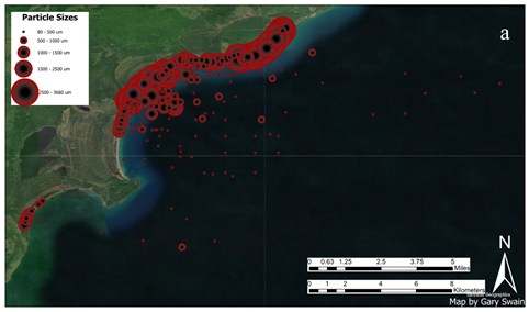
Bay Particle Size Distributions. Not surprisingly, in mixed sand grain samples across the bay, mean particle size varies greatly with water depth, current strength, and wave action (Figure 15a; also check [58]). Detailed data for particle size distributions in Grand (Big) Traverse Bay are found in Supplementary Appendix Tables S1 and S2 for sieved beach and sediment (Ponar) samples. The largest particles, ranging from fine gravel to sands (3 mm-600 um), were found along stamp sand beach deposits, especially at the Gay Pile site and near the Traverse River Seawall, the latter where wave action was most pronounced. Natural white sand (quartz) beach particles (lower Grand/Big Traverse Bay; Little Traverse Bay) were slightly smaller (peak 600-800 µm) and more uniform from site to site. Underwater, from shallow shoreline samples out across the shelf region, the two particle types, stamp and natural sands, were fairly similar in size frequency distributions (Figure 8b). Plotting values across Grand (Big) Traverse Bay, off the escarpment edge and into deeper waters, sizes were smaller, moving to silt and clay-sized fractions in deep water. Deep sediments also included more fine organic matter.
 |
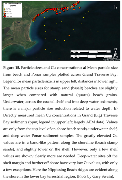 |
Mapping Stamp Sand Percentages (Particle Counting Method) Along Beach Shorelines And Across The Coastal Shelf Region. To better understand where stamp sands from the main tailings pile dispersed throughout the bay, around 175 sediment samples were taken using Ponar grabs between 2008 and 2019 (Figure 5b; Supplementary Appendix Tables S1 and S2). The percentage stamp sand determinations (Figure 16a) come from the microscopic grain-counting technique (see Methods). The highest values (80-100% SS) are from stamp sand beach deposits between the original Gay Pile site and the Coal Dock. The second highest percentages are around the Traverse Harbor region. Underwater, the high percentage band extends out around 0.5-1 km offshore and includes large migrating underwater stamp sand bars (Figure 5a–c) dumping into the northern portions of the “Trough”, the ancient river bed. In addition, there are fields of stamp sands moving from the “Trough” into northeastern cobble beds of Buffalo Reef. To the southwest, past the Coal Dock region, slightly lower percentages occur nearshore down to the Traverse River Harbor. Reduction of stamp sand percentages occurs because migrating stamp sands encounter a bedrock high and also mix a bit with natural quartz sands, which still cover much of the lower bay.
In the Traverse River Harbor region, shoreline stamp sands also moved underwater offshore south-eastward into a depression on the western flanks of Buffalo Reef (Figure 5a, site #7). For the last century, the Coal Dock and Harbor Seawall at the Traverse River outlet acted like groins (right-angle barriers), capturing and slowing coastal stamp sand migration down the beach from the Gay Pile. Unfortunately, recent sampling just past the Harbor Seawall into the Lower Bay and along the natural quartz beach has revealed some stamp sands (Figure 8a; Figure 16a), causing concern that stamp sands are beginning to move around the Seawall and into the lower portion of the bay [7,29,50,54]. In the lower bay, the original narrow white quartz beach extends from a Nippissing Beach series. Dating of the complex [96] indicates continuous deposition of natural sand in the southern region of the bay for thousands of years (3800-900 years) with a strandline progradation rate of 0.68m yr-1.
 |
Maps of stamp sand percentages contoured across the bay (Figure 16a) show percentages of stamp sand decline in water depths out two km from the shoreline across the shelf region to the escarpment drop-off. However, a few migrating stamp sand bars are perched periously close to the edge of the shelf (Figure 5a,b). Beyond the shelf edge, especially in Outer Bay deep waters (50-200m), percentage stamp sand values are quite low (often < 10%). Deep-water sediments beyond the escarpment are normally dominated by silt and clay-sized particles, often with organic additions (diatom tests, plankton, pollen grains, benthos), so our grain-counting technique requires sieving to retrieve appropriate sand-sized grains for cross-comparisons (again underscoring that this technique is not really suited for deep-water silt-sized sediments; see Methods). Moreover, spring shoreline ice occasionally transports stamp sands out to deeper waters [7,97] and melts to produce “salt and pepper” particle patterns in sediments.
Reduction of the slime clay fraction in redeposited beach stamp sand deposits is evident from sieving studies (Supplementary Appendix Table S3) and is independently noted by both NRRI [98] and USACE ERDC-EL, Vicksburg [95]. Because of spatial concerns, we made two attempts to directly determine Cu concentrations directly in samples. The first was from our pre-2019 Ponar sediment samples (N = 40) and the second was during the 2019-2022 AEM Project (N = 132 samples).
If the percentage of stamp sands is known in mixtures of beach and shelf sands across the bay, and if copper is retained within dispersing particles, there is an opportunity to predict Cu concentrations in beach and coastal shelf deposits. Recall that we used the MDEQ value of Cu at the Gay Pile as a standard (2863 ug/L or ppm), multiplying percentage stamp sand times that value to derive preliminary estimates of Cu in sediment sand mixtures [29]. However, as mentioned earlier, there were concerns about such simple calculations. The first was that more dense particles with higher copper might settle closer to the pile location. The second involves the clay-sized particle fraction (7-14%) in the Gay Pile [42]. The clay fraction in the pile is known to have a higher concentration of copper than the sand-size fraction, around 4,680 ppm [27,98]. If clay-sized particles are winnowed out by waves along the shoreline, some slime clays might be captured in Buffalo Reef crevices, or move out of the bay. Copper concentrations in coastal stamp sands would probably decline farther from the Gay Pile source.
Predicted Copper Concentrations Versus Direct Determinations. During 2008 to 2019, copper concentrations were determined at ca. 40 bay sites, primarily from shelf Ponar samples. A linear regression was fit to a plot of copper concentration (Y axis, in ug/g or ppm) vs % stamp sand (X-axis). The N=40 point linear regression was Y = 25.066X – 156.4, highly significant with an F value of 246, and a p value of 3.328E-18 (Table 3). The R2 value was 0.867, with a multiple correlation of 0.931. However, the linear regression fit had a Y intercept value of -156 with a standard error of 65.7 ppm, suggesting some low-end interference, perhaps from natural magnetite grains mis-identified as stamp sand particles. To compare against our standard value of 2,863 ppm from the Gay Pile site (MDNR), we solved the equation for the Y intercept value at 100% SS and obtained 2,350 ppm, only 82% of the Gay Pile value (Table 3).

Table 3.
Cross-comparisons of various regression lines for Grand (Big) Traverse Bay; Cu concentrations are plotted against percentage stamp sands (%SS). The MDEQ standard for the Gay tailings Pile is 2,860 ppm (N = 247) for 100% Stamp Sand. The first regression is the original calibration curve regression from [29]; the rest are from the AEM Project.
| Source | N | R2 | Regression Equation | 100% SS Intercept (ppm) |
|---|---|---|---|---|
| Initial Cu Calibration Kerfoot 2021 | 40 | 0.867 | Y = 25.066X - 156.43 | 2350 |
| AEM Mean Regression, All SS | 10 | 0.812 | Y = 17.838X + 271.61 | 2055 |
| AEM, All Under 50% SS | 63 | 0.475 | Y = 28.699X - 17.965 | 2852 |
| Along Shoreline Under 50% SS | 36 | 0.61 | Y = 33.019X + 37.744 | 3340 |
The AEM Project provided an excellent independent opportunity to check if relative Cu concentrations remained similar in stamp sand percentages across the entire bay, as particles were dispersed spatially by waves, currents, and ice. However, for regression analysis of the data, there were some issues with heteroscedasticity (see Methods) that required statistical attention. To avoid heteroscedasticity, for the entire data set (N = 132), mean %SS values were plotted against corresponding mean Cu concentrations at 10% SS counting intervals (e.g., 0-10%, 10-20%, 20-30%, and so on up to 90-100% on the x-axis). There was relatively good correspondence (Figure 17a) between the two mean measures (R2 = 0.812, i.e., a correlation of r =0.901; regression F = 25.9, p = 0.00094). The regression equation was y = 17.838X + 272, with little evidence of heteroscedasticity. The predicted 100%SS intercept value was slightly lower, 2056 ppm, only 72% of the Gay Pile MDNR standard (2,863 ppm). Recall that the entire AEM data set was dominated by beach samples and cores, as compared to just Ponar sediment samples, in the N=40 regression. The standard error of the intercept value was around 261, indicating a significant departure.
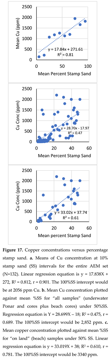 |
Additional regressions were plotted from the AEM data, allowing multiple comparisons between % SS and corresponding Cu concentrations, in addition to estimates of intercept values at 100% stamp sand. For example, looking at individual points, we reduced heteroscedasticity by plotting only the values between 0-50% stamp sand percentages for the whole set. In this case, the correlation was lower, but still highly significant (R2 = 0.475; correlation r = 0.689) and the regression was y = 28.699x - 17.965 (Figure 17b; Table 3). The regression intercept at 50% was 1,417 ppm, which translated into an intercept of 2,852 ppm at 100%, very close (99%) to the Standard (MDEQ Gay pile) value of 2863 ppm. Another regression, Cu concentrations for “on land (beach)” values only, between 0-50%, also gave a decent correlation (R2 = 0.610, r = 0.781) and a regression of Y= 33.019X +37.744. At 50%SS, the intercept was 1,689 ppm Cu; equivalent to 3,340 ppm at 100% stamp sand, slightly above (120%) the Gay pile value (Figure 17c; Table 3). The latter set incorporated a great range of historical mixtures, as cores punched down into underlying natural beach sands, reaching low values of % SS. If all the intercept values (N=4) from Table 3 are averaged, the mean is around 2,649, only slightly below (93%) the standard Gay Pile value.
A plot of surface Cu concentrations in beach and underwater sediments across Grand Traverse Bay (Figure 15b), shows very high surface concentrations along the beach stamp sands in a band from the Gay pile to the Traverse River Seawall (500-4,500 ppm). Copper concentrations are also relatively high immediately offshore, along the migrating stamp sand bars between the Gay Pile and where they spill into the northern portion of the “Trough”, and in NE cobble fields of Buffalo Reef. Intermediate concentrations are present across the shelf region west of Buffalo Reef, but more spatial cover is needed for contouring. There is again evidence of leakage around the Seawall area into the southern bay. Concentrations drop to relatively low values (3-100 ppm) in deep water sediments off the shelf region.
Breaking the AEM sets of samples into three regions: stamp sand beach, shelf, and off the escarpment into deep-water regions of the bay (Figure 15b; Supplementary Appendix Table S1), there are clear differences in particle-specific Cu concentrations. Beach stamp sands had relatively high values of Cu close to the Gay Pile, but also relatively high values along the entire shoreline. Copper concentrations in shelf sediment samples are lower, mainly because stamp sand percentages are lower, yet the predicted relative Cu values per particle are relatively close (87% of the expected Gay Pile standard). Deep-water Ponar sediment samples have low Cu values again because stamp sands percentages are low in sediments, but here there are significant departures from the predicted particle Gay Pile Standard. For example, for N = 12 values from deep-water, mean predicted particle Cu concentrations were predicted to be 94 +/-31 ppm 95% C.L., yet observed Cu particle concentrations were significantly lower (52+/- 42 ppm 95% C.L.). Thus in deep water sediments, the observed Cu concentrations in sand-sized particles were only 56% (0.56 +/-0.30 95% C.L.) with significant departure from the predicted value. Perhaps the deep-water sand-sized particles include components from multiple sources, e.g., glacial lag sand or river discharges.
Others have noted a decrease in copper concentrations in some sites farther away from the main Gay Tailings Pile site. MDEQ (2006) noticed a lower value for copper at the Traverse River Seawall (1,443 ppm Cu) than at the Gay pile (2,863 ppm). Additional sampling by NNRI [98] also detected a comparable decrease in Cu concentration at the Traverse River Seawall site (1,210 ppm) compared to the Gay Tailings Pile (2,863 ppm) standard. However, recent ERDC sampling at three beach sites (Gay Pile, Coal Dock, Harbor Seawall) found copper concentrations of 3,460 ppm, 2,400 ppm, and 2,810 ppm, similar to the AEM results and the MDEQ Standard.
Leaching Studies, Transfer Of Cu To Interstitial And Pond Waters. For environmental assessment, even with excellent characterization of stamp sand distribution within the bay, additional studies are essential to answer key questions: 1) how much of the Cu is retained as stamp sand particles disperse; 2) as stamp sands are agitated or subjected to seepage waters, how much Cu is lost as fine particulate or dissolved Cu, and 3) are the concentrations toxic to aquatic organisms? Relative to toxicity, we must remind ourselves that stamp sands contain not only high concentrations of Cu, but also additional metals (Table 1) that might flag state and agency standards.
In preliminary leaching studies with shaken stamp sands, we recorded Cu, Al, and Fe concentrations as well as TOC (Table 4). Relative to Cu, recall that concentrations in stamp sand particles are usually recorded in parts per million (ppm), whereas releases, i.e., fine particulate and dissolved concentrations, are listed as parts per billion (ppb; µg/L), underscoring that relatively small amounts of copper are released into water from stamp sand particles. In our tests, only 330-550 ppb of “total Cu” were released in agitation experiments compared with 2863 ppm occuring within stamp sand particles (i.e., only 0.0001-0.0002% of total mass). This ten-thousand-fold difference underscores that dispersing stamp sand particles retain most of their copper. High concentrations of fine particulate and dissolved copper came from stamp sands agitated in Traverse River and Coal Dock stream waters. These waters had the lowest pH and highest DOC/TOC (tannins). Moreover, the concentrations of total Cu released into rinse waters were high relative to potential toxic effects on aquatic organisms. When we followed up with 0.4 µm filtration to separate out the dissolved fraction from the total, values were lower (60-240 ppb), but still highly toxic levels for many aquatic organisms. The preliminary experiments were intended to simulate what might be moved into pond and interstitial waters when stamp sands are agitated, either by wave action in ponds, ground-water seepage through beach stamp sands, or as dredged material pumped through pipes into the Berm Complex.
Table 4.
Metals leached from stamp sands (Gay Pile) over one week of periodic agitation. Water sources listed in first column. Concentrations of Al, Cu, and Fe in ppb, determined by Perkin Elmer Optima 7000DV ICP-OES. Calculated as total metal differences from original water versus agitated stamp sand. Total organic Carbon (TOC) from Shimadzu TOC-LCPH Analyzer (MTU AQUA Lab).
| Water Source | Al 394 (ppb) | Cu 327 (ppb) | Fe 238 (ppb) | TOC (mg-CL-1) |
|---|---|---|---|---|
| Lake Superior (LS) | 480 | 330 | 933 | 1.8 |
| Bete Grise (BG) | 525 | 515 | 527 | 1.5 |
| Portage Lake (PL) | 510 | 330 | 760 | 1.5 |
| Traverse River (TR) | 430 | 550 | 853 | 13.9 |
| Coal Dock (CD) | 520 | 515 | 739 | 21.2 |
| Cu mean = 448 (SD = 109) | ||||
ERDC-EL leaching experiments were more extensive and included sequential tests, to see if released amounts declined with time (e.g., if surface rimes were removed with multiple rinses). Again, the total amounts of dissolved Cu leached were orders of magnitude less than the solid phase copper concentrations in bulk stamp sands. In ERDC-EL tests with multiple rinses, the leachable Cu fraction was higher, but still only about 0.043-0.068% of total Cu mass (thousand-fold difference).
Our and ERDC-EL measurements of existing suspended total copper (fine particle plus dissolved Cu) in various ponds from the Stamp Sand Pond region were variable and are listed in Table 5. The 2019 field survey, before “Berm” construction, found “total copper” values ranging from a low of 50 ppb to a high of 2,580 ppb (mean = 575 ppb; SD = 697; SE= 184). The mean for pond waters fell within the confidence limits for total copper values from agitation experiments. After “Berm” construction, in 2022, ERDC found a seepage pond adjacent to the outer rim of the berm to have a total Cu concentration of 1,710 ppb, whereas berm disposal waters were even higher (total copper = 2,850 ppb). Thus the second major conclusion is that amounts of Cu released into pond and interstitial waters are very high for stamp sand beaches, relative to potential toxic effects on invertebrates and YOY fishes.
Table 5.
Aluminum and Copper concentrations in water samples from several stamp sand beach ponds (“Pond Field”) near Gay (2019 MTU sampling). Concentrations are for “total” (fine particulate and dissolved). Latitude and Longitude location by GPS. MTU metals analysis from Perkin Elmer Optima 7000DV ICP-OES.
| Pond Number | Latitude | Longitude | Al 396 (ppb) | Cu 327 (ppb) |
|---|---|---|---|---|
| P1 (2019) | 47.16781667 | -88.17075000 | 70 | 990 |
| P2 | 47.21850000 | -88.17008333 | 50 | 270 |
| P3 | 47.21896667 | -88.16863333 | 40 | 120 |
| P4 | 47.21825000 | -88.16753333 | 50 | 80 |
| P5 | 47.21736667 | -88.16800000 | 10 | 70 |
| P5B | 47.21653333 | -88.16900000 | 10 | 60 |
| P6 | 47.21605000 | -88.16833333 | 20 | 50 |
| P7 | 47.21551667 | -88.17040000 | 20 | 90 |
| P8 | 47.21671667 | -88.16781667 | 130 | 200 |
| P9 | 47.21713333 | -88.17045000 | 150 | 2580 |
| P10 | 47.21441667 | -88.17800000 | 80 | 950 |
| P11 | 47.21463333 | -88.17698333 | 290 | 940 |
| P12 | 47.21346667 | -88.17868333 | 30 | 860 |
| P13 | 47.21398333 | -88.17888333 | 30 | 790 |
| Mean Concentration | 70.0(76.3) | 575(696.7) | ||
| ERDC 2021 | ||||
| “Edge pond” | 1710 | |||
| “Berm” | 2850 | |||
Field Incubation and Laboratory LD50 Experiments With Daphnia. As an example of toxicity for invertebrates, our field experiments checked survival of native Daphnia in a set of ponds surrounded by beach stamp sand deposits (Pond Field). That is, where interstitial waters seep into ponds and elevate Cu concentrations. A total of four racks, each with forty Daphnia collected from neighborhood forest ponds, were deployed in stamp sand ponds located slightly south of the Gay tailings pile. For the Control, one rack was deployed from the MTU Great Lakes Research Center (GLRC) dock into Portage Lake water.
Results at the two sites (Stamp Sand Field Ponds, Control) could not have been more different. At the control site (GLRC dock), the incubation lasted the full two weeks. Daphnia survival was 97.5% (39 of 40 Daphnia survived), and the accumulative number of offspring produced totalled 295 juveniles. In contrast, Daphnia survivorship was zero after two days in three stamp sand ponds (Figure 18). At the remaining pond (Pond #1), only 1 Daphnia survived for three days. Moreover, no offspring were produced in any pond.
Figure 18.
a. Daphnia pulex survival and fecundity in Portage Lake water, off the Great Lakes Research Center (GLRC) dock. Survival percentage (97.5%) is based on forty adults suspended in individual vials with mesh for water exchange. The 100µm mesh allowed local waters, phytoplankton, and nutrients into vials, but prevented predators and escape of Daphnia. The accumulative number of juveniles born is also plotted against time (295 young). b. Daphnia pulex survival and fecundity in vial racks suspended in Gay stamp sand ponds. Again, survival percentage is for adults in 40 vials. In contrast to our Control (Portage Lake), there was no viable production of young. Again, the design was identical to the Control, as vials were covered by a 100µm mesh that allowed local waters, phytoplankton, and nutrients in, but prevented predation and escape of the enclosed Daphnia.
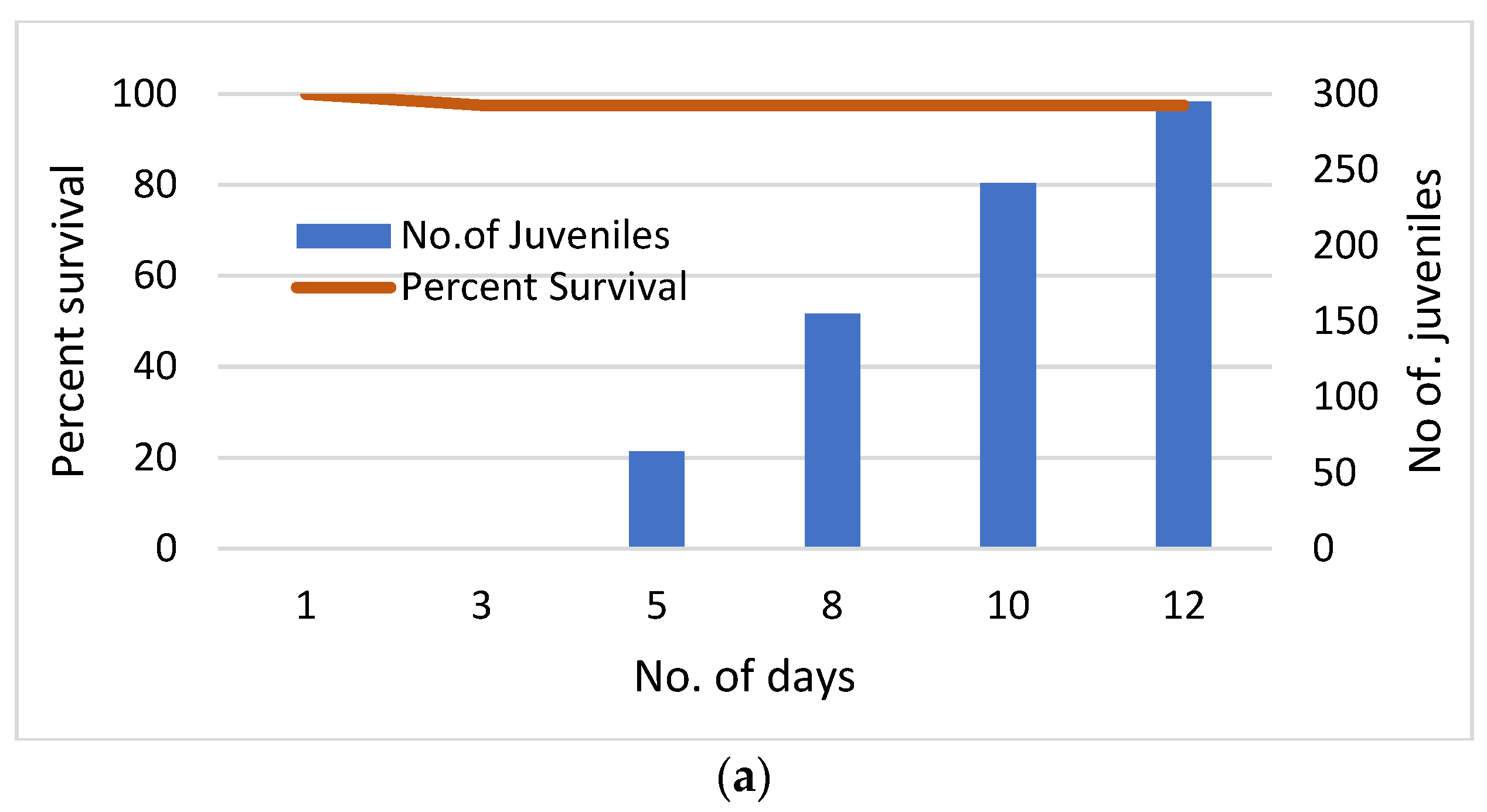
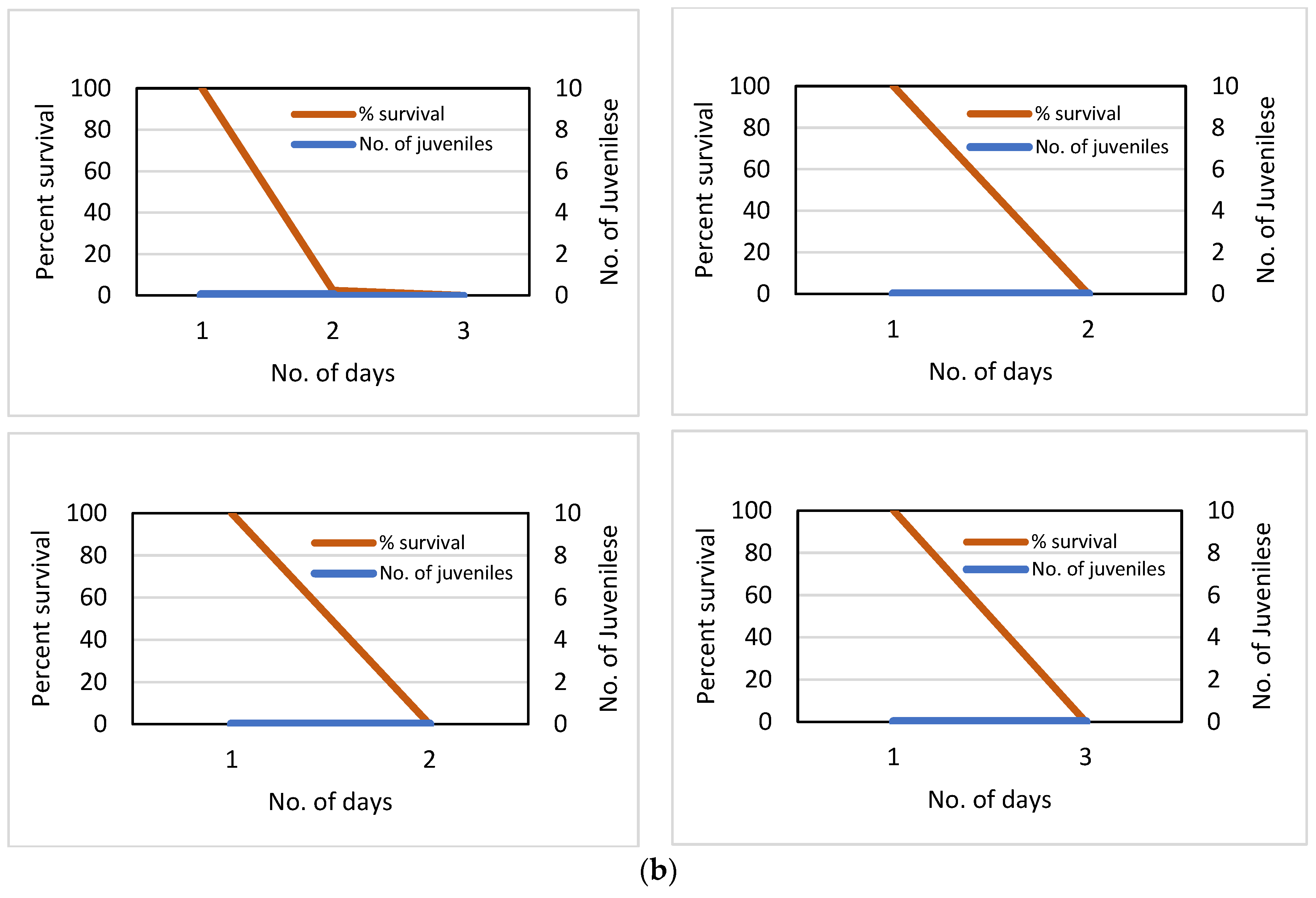
LD50 tests were also run on Daphnia at the GLRC Lab. Subsamples from our theoretical 1,000 ppb Cu stock solution were checked at the LEAF lab. Values turned out to have a mean concentration of 790 ppb, which required a slight readjustment down from our original 1,000 ppb, 500 ppb, 250 ppb, 100 ppb, 50 ppb, 25 ppb, 10 ppb, 5 ppb, and 0 ppb sequence. Application of the probit regression approach for determining an LD50 value estimated 8.9 ppb for Daphnia magna [99]. In the Discussion, we compare this value with other published Daphnia values and our earlier 1999 lab tests, and find the values very similar and all low. Clearly, concentrations of total and dissolved Cu in interstitial and pond waters were highly toxic to common invertebrate taxa like Daphnia.
4. Discussion
Several copper mining operations (examples in Table 1) continue to discharge copper-rich tailings into river or coastal environments. Although banned in the Great Lakes of Canada and the USA since the Clean Water Act of 1972, there remain many “legacy” (iron, gold, and copper) sites around the Great Lakes Basin where tailings are confined behind river coffer dams, or placed in excavations that eventually could collapse and contaminate watersheds. In Chile, because of increasing copper demand, the current 800 MMT per year of tailings production could nearly double by 2035 [100]. Since 2014, there were four major global tailings dam failures that killed hundreds of local residents and severely contaminated environments: Mount Polley, Canada (2014); Fundao Samarco, Brazil (2015); Corrego Do Feijao Brumandinho, Brazil (2019); and Jagersfontain, South Africa (2022). As a consequence, an international effort [International Council On Mining and Metals [ICMM), UN Environmental Program, and the Principles For Responsible Investments (PRI)] developed a “Global Tailings Management Standard For the Mining Industry”. That Standard was launched in August 2020, and urges adoption by mining companies world-wide [101].
As shown in the Buffalo Reef Project, technical advancements in remote sensing have created new options for environmental assessments, allowing us to “see” beneath bay and oceanic waters, quantifing both detailed elevation and bathymetric features of coastal margins. Geospatial surveys (aerial photography, LiDAR, multispectral studies, conventional and triple-beam sonar, side-scan sonar, ROV, drone photography and instrument package surveying, sediment coring) seem indispensible for characterizing coastlines, e.g., including encrochment of stamp sands onto Buffalo Reef. After years of planning, the Buffalo Reef Project moved into initial remediation steps (Stage 1) during 2017, with 5-Agency (EPA GNPO, MDNR, Army Corps of Engineers, GLIFWC tribal) initial funding of around $7.5M. Challenges past Stage 1 dredging, geospatial surveys, and planning for the Project included: 1) determining short-term and long-term toxic environmental effects, 2) measures to protect Buffalo Reef against migrating tailings, and 3) constructing a place for stamp sand removal and disposal. In addition, there is a priority for finding regional applications for stamp sands that are benign.
General Properties Of Tailings (Stamp Sands) With Some Suggested Applications. Density/specific gravity calculations indicated that stamp sand particles, which are pulverized basalt (a silicate), are slightly denser than natural quartz beach grains, which erode locally from the Jacobsville Sandstone bedrock. Specific gravity differences at field type locations (Stamp Sand= 2.88 g/cm3 vs Natural Sand= 2.55g/cm3) were statistically significant, but only with differences of 9-12% total mass. Due to mining discharges, mixtures of stamp sand and natural sand occur extensively along bay shorelines, inland lakes, and river edges of the Keweenaw Peninsula.
Simultaneous studies at the USACE ERDC-EL lab in Vicksburg [95] independently documented many properties of stamp sands. ERDC found that stamp sands were nearly all sand size, yet the original pile also contained gravel size and clay-sized fractions. The clay-sized fraction amounted to nearly 10% at the original Gay tailings pile (< No. 200 sieve, 9.3%). In contrast, stamp sands that eroded onto beaches down-drift of the Gay pile were more uniform than those at the original Gay pile. Stamp sands had engineering properties comparable to natural sands in terms of voids content, soundness, density, absorption, California bearing ratio, and angle of repose. Some researchers suggested using stamp sands as aggregate for concrete [102]. Years ago, concrete cinder blocks were manufactured at Superior Block Company in Houghton using stamp sands from the Isle Royale pile as an aggregate. Unfortunately, ERDC found that sorted beach stamp sands would probably require additional processing to meet the fine aggregate size distribution for concrete. However, use with asphalt has also been suggested, as has use as road bedding, e.g., Weston Solutions independently suggested road bed application. ERDC stated that beach stamp sands were too uniform and rounded for aggregates, whereas gravel and fines needed to be removed from the main Gay pile material to make material adequate for aggregates. Weston Solutions also felt stamp sands appeared physically suitable for fill, a use common around the Peninsula, as well as for road ice treatment during winter [103,104]. Moreover, ERDC documented that wave-worked beach stamp sands had much lower clay content in addition to the strong size sorting, verifying removal of slime-clay fractions by wave action, plus found an angle of repose of 33% slope.
Water Quality Concerns Relative To Tailing’s Cu Leaching. Michigan “stamp sand” toxicity has now been explored by numererous agencies. Recall that the concentration of Cu in Gay Pile stamp sands was 0.28% of mass. At an extensive Gay tailings pile site sampling in 2003, several metals were found to exceed the State of Michigan Groundwater Surface Water Interface Criteria (GSWIC) levels (Michigan Department of Environmental Quality, [105]). The sampling included 274 soil samples. Aluminum exceeded levels in 271 samples, chromium in 265, cobalt in 271, copper in 274, manganese in 159, nickel in 168, silver in 216, and zinc in 242. In ten groundwater samples, the number of metals exceeding GSWIC risk criteria for dissolved metals included: chromium 5, copper 10, manganese 5, nickel 8, silver 8, and zinc 8. In 2003, MDEQ also collected stamp sands from a southern redeposited stamp sand beach site, north of the Traverse River Seawall (N= 24 samples). Here copper averaged lower, 710-5300 μg g-1 (mean = 1443 μg g-1, or ppm) than at the Gay site. But in the 25 samples, various other metals again exceeded GSWIC levels: aluminum in 20 samples, chromium in 19, cobalt in 24, copper in 24, manganese in 7, nickel in 8, silver in 9, and zinc in 10 [105]. However, Weston Solutions testing [83] showed that only copper (total concentrations) exceeded surface water quality criteria in both porewater (interstitial) and pond waters. Whereas total suspended metal concentrations of chromium, lead, manganese, nickel, silver, and zinc in porewater exceeded surface water criteria, their dissolved concentrations did not exceed criteria, suggesting copper and perhaps aluminum water releases were the most important relative to toxicity.
Recent ERDC studies also looked at elemental concentrations within stamp sand beach deposits, at three separate sites: Gay Pile, Coal Dock, and against the Traverse Seawall [95]. Fewer measurements were made than in the earlier MDEQ series, consequently there was greater variability. Because basalt is an aluminum, calcium, magnesium silicate, these elements were especially abundant. Whole sample copper concentrations at the three sites were 3,460 ppm, 2,400 ppm, and 2,810 ppm, similar to AEM results. Elements exhibited the following ranges: aluminum (12,700-14,700 ppm); arsenic (5.52-6.39); cadmium (0.405-0.544); calcium (18,100-32,200); chromium (15.8-24.0); cobalt (26.4-31.3); lead (2.39-3.68); lithium (5.59-6.23); magnesium (16,100-17,800); manganese (389-459); nickel (24.4-26.0); selenium (1.90-2.76); strontium (11.6-21.6); and zinc (57.9-68.7).
ERDC also conducted runoff tests for stamp sand beach deposits following USACE Upland Testing Manual (2003) techniques, using an agitated solids concentration of 5000 mg/L (i.e., 5,000 ppm). The simulated runoff water exceeded both acute and chronic water quality criteria for copper with a maximum dissolved mean concentration of 206 ppb. Over the range of pH conditions, the maximum total copper concentration was released at pH 4.2, and lowest at pH 7. Of the other metals, aluminum occasionally exceeded chronic and acute toxicity levels. Cadmium, selenium, and silver exceeded lower chronic toxicity criteria [95].
In the ERDC studies, runoff water quality was evaluated for three size fractions and solids concentrations of 250, 500, 1500, 5,000 15,000, and 50,000 mg/L (ppm) with challenge waters of pH 4.2, pH 7, and saline pH 7. The runoff water exceeded both the acute and chronic water quality criteria for copper, and occasionally for aluminum, in the pH 4.2 and saline pH 7 challenge waters. Median dissolved Cu concentrations released were 146-430 ppb. Multiple leaching (rinsing) tests showed that dissolved copper concentrations generally decreased for stamp sand samples with multiple rinses, yet challenge waters remained greater than the water quality criteria (WQC) for chronic toxicity. Of the other elements, although lead and zinc also decreased throughout leaching cycles, both elements occasionally exceeded WQC levels for chronic toxicity. Another important result was that in the presence of reasonable concentrations of DOC (20 mg/L), leachability of Cu in stamp sand was increased by about a factor of 25, and the partitioning coefficient was also increased by about a factor of 18. Consequently, the leaching of copper in the presence of DOC is likely to persist about 20 times longer than in the absence of DOC. This result supports the initial findings of Jeong et al., 1999, that when tannin-rich forest groundwater moves through stamp sand, it accelerates the leaching of dissolved Cu into the stamp sand beach ponds and along the shoreline margin.
ERDC also checked the transport of Cu during dredging, followed by deposition into “retaining ponds surrounded by stamp sand berms” (Figure 12). Concentrations in the dredging slurry released into the receiving “Berm Complex” were sampled, as well as seepage through berm walls into outlying ponds. Total Cu concentrations in elutriates, Berm, and pond waters ranged between 234-2,120 ppb, whereas dissolved Cu varied between 24-117 ppb. Concentrations for total aluminum were 1.81-4.73 ppm, with dissolved Al at 53-251 ppb. The Cu concentrations were all above acute and chronic toxicity values, whereas the Al total concentrations were also above acute and chronic toxicity levels. For copper, ERDC used acute and chronic toxicity levels of 13.0 ppb and 9.0 ppb, respectively. For aluminum, they were 87 ppb and 750 ppb. Manganese and selenium also occasionally flagged chronic toxicity levels [95].
In summary, both our and ERDC leaching experiments revealed that almost all of the copper mass is retained within dispersed stamp sand particles. This is why migrating particles across the bay remain toxic, and why the initial percentage stamp sand prediction of copper concentrations was spatially useful. However, as particles moved away from the eroding Gay tailings pile, AEM results showed slightly lower concentrations of copper, again confirming some particle sorting during dispersal.
Arsenic Toxicity Issues:“Mohawkite” Milling. Globally, the most dangerous chemical elements for human beings in copper tailings are arsenic, lead, cadmium, and uranium [106]. Recent references to an arsenic-rich copper mineral “Mohawkite” (actually a combination of mixtures of arsenic, silver, nickel, skutterudite and copper; varying between Cu3As to Cu6As) found during early Mohawk Mine operations require comments. Mohawkite is a fascinating rock, collected by gem hunters from Mohawk Mine poor-rock piles and fashioned into belt and tie ornaments. Emphasis upon high levels of arsenic originating from Mohawk Mill operations, however, is largely unfounded, for the bulk of the “Mohawkite” ore was processed separately from the routine copper milling operations at Gay. Consequently, the concentration of arsenic in stamp sands from the Gay pile is hardly more than amounts found in stamp sands from other amygdaloid mining sites (Table 1; [27]). Documents in MTU Archives record that the Mohawk administrators were aware of the potentially hazardous effects of processing such arsenic-rich copper material at the Gay Mill site, yet wanted profits from the metal-rich ore. Mohawkite deposits were first found on Jan 1, 1901 on the 1st level of No. 1 Mohawk Shaft. About 70 tons were sent to Swansea, New York for reducing, yielding $140/ton. Due to the large amounts of arsenic, it was difficult to smelter (produces arsenic fumes). Consequently, a special smelter was constructed at Hackensack Meadows, New Jersey, and put into commission during the fall of 1901. At the Mohawk Mine, a 2nd and 3rd vein of Mohawkite was found in Shaft 2. In 1901, the load amounted to 230,000 lbs. In 1902, 700 tons were sent to New Jersey for reduction. The new smelter was given an arrangement that the mine would provide 100 tons Mohawkite ore per month from 4 shafts for three years. There are no records of Mohawkite “ore” specifically being processed at the Mohawk or Wolverine Mills, although small amounts of the mineral Mohawkite are recorded from many mine locations in the Keweenaw [see Special Issue: “Michigan Copper”, The Mineralogical Record, January-February 2023; Vol. 54 (1) 196pp]
Field & Laboratory Acute Toxicity Tests. Toxicity tests were run on several small stamp sand beach ponds south of Gay, in addition now to the “Berm Complex” that received dredged material from both the Traverse River “over-topping” and from the “Trough”. Our preliminary leaching experiments with stamp sands suggested an initial release of around 300-600 ppb total Cu into waters when stamp sands were agitated with water (range 330-590 ppb, mean 448 ppb). Direct measures of total Cu in 13 ponds (range 50-2,580 ppb; mean 575 ppb) were comparable, if not slightly higher. When Daphnia were submersed in stamp sand pond waters at 4 sites, most died within 48 hours and produced no young. Our acute toxicity tests (LD50%) showed that values as low as 8.6 ppb dissolved copper would kill Daphnia. The rapid death of Daphnia in waters that range from 50 to over 2,000 ppb total Cu is thus no surprise. Moreover, our acute toxicity values for Daphnia correspond closely with literature values for different Daphnia species and our previous 1990′s determinations (Table 6).
Table 6.
Results of Acute Toxicity Tests of Cu (48hr LD50) on Pelagic Cladocera. The list is largely compiled by Brix et al. 2001. Our findings are included with an asterisk (*).
Table 6.
Results of Acute Toxicity Tests of Cu (48hr LD50) on Pelagic Cladocera. The list is largely compiled by Brix et al. 2001. Our findings are included with an asterisk (*).
| Species | N | LD50 (ppb Cu) |
|---|---|---|
| Ceriodaphnia reticulata | 1 | 5.2 |
| Daphnia ambigua | 1 | 24.8 |
| Daphnia magna | 12 | 18.1 |
| Daphnia parvula | 1 | 26.4 |
| Daphnia pulex | 2 | 8.8 |
| Daphnia pulicaria | 8 | 9.3 |
| Daphnia pulex* | 3 | 7.7 |
Around the late 1990s, our laboratory also performed LD50% tests on local Daphnia pulex [88,89]. They also ran comparable immersion experiments in the Gay stamp sand ponds at that time and measured dissolved Cu in pond waters. In the lab, three separate experiments with native D. pulex gave results of 9.4+/-0.1 ppb, 3.6+/-0.5 ppb, and 10.4+/-2.0 dissolved Cu for LD50% levels. Moreover, total Cu measured in several of the then 26 stamp sand ponds ranged from 45-1,712 ppb, with a mean of around 440 ppb, close to but slightly lower than the present (2019) survey. Daphnia pulex (from neighborhood forest pond waters) placed in submersed vials at that time also died rapidly relative to control sites. The main point is that interstitial and pond waters have remained highly toxic to aquatic life for over 25 years of testing at the pond site. If anything, survival and fecundity back in the late 1990′s was slightly better than recently, for there was some fecundity and a several individuals survived over 24-48 hours [88,89]. Statistical comparisons of past and present pond experiments do show slight, but significant differences between 1990 and 2019 results [99]. ERDC measurements of Cu toxicity levels are also higher now in the pond field, probably related to leakage of dredged material from the “Berm Complex”.
Toxicity Results With Other Invertebrates & Fish. A variety of agency and institutional tests of stamp sand-contaminated sediments from the Keweenaw, as well as specific tests with Grand (Big) Traverse Bay sediments, have additionally demonstrated toxic effects. Here the EPA test results include not only crustaceans, but a variety of benthic invertebrates. Freshly worked stamp sands in lake sediments were toxic to Daphnia and mayflies (Hexagenia) because they released Cu across the pore-water gradient [107]. Additional laboratory toxicity experiments with stamp sand-sediment mixtures at EPA-Duluth [108,109,110] showed that solid phase sediments and aqueous fractions (interstitial water) were lethal to several taxa of freshwater macroinvertebrates: chironomids (Chironomus tentans), oligochaetes (Lumbriculus variegatus), amphipods (Hyalella azteca) and cladocerans (Ceriodaphnia dubia). In the latter studies, the observed toxicity was almost exclusively due to copper, not other metals in the secondary suite (principally zinc and lead). Weston Solutions [83] toxicity studies in Grand (Big) Traverse Bay tested Ceriodaphnia dubia, Hyalella azteca, and Chironomus. They utilized dilutes with five sediment samples from the Gay pile and the southward stamp sand shoreline. All sediment samples showed acute and chronic effects (growth, reproduction) on benthic organisms.
In even more recent MDEQ investigations [104], six sediment locations were sampled along the Gay to Traverse River shoreline transect. Solid phase copper concentrations varied between 1500-8500 μg g-1 (mean 2,967 ppm), whereas the secondary suite had: Ag 1.2–1.7 μg g-1 (mean 1.5), As 1.7–3.1 μg g-1 (mean 2.2), Ba 6.6–8.6 μg g-1 (mean 7.7), Cr 31–39 μg g-1 (mean 35), Pb 2.1–2.9 μg g-1 (mean 2.6) and Zn 62–79 μg g-1 (mean 72). Bulk sediment toxicity testing showed that all six sediment samples from the shoreline were acutely toxic to both Chironomus dilutes and Hyalella azteca. Two samples were taken just south of the Traverse River harbor in a largely white sand bottom with a little stamp sand that also had excessive solid phase copper concentrations (300-400 μg g-1), whereas one sample farther down the white beach had much lower solid phase concentrations (79 μg μg g-1). The latter two sample sites were not tested for toxicity.
In the recent ERDC Vicksburg tests, the Army Corps [95] also ran additional suspended and dissolved phase toxicity tests on supernatants from each of the elutriate tests concerning dredging material released into the berm complex. Both acute (48- and 96-hr) and chronic (7-day) toxicity tests were run using the daphnid Ceriodaphnia dubia and the fathead minnow (Pimephales promelas). Additional tests were run on filtered elutriates of the original Gay pile stamp sand and unfiltered pond water from the berm dredging ponds. The results showed that untreated and undiluted effluent was likely to be acutely toxic, and would require great dilution to eliminate toxicity. Disposal (berm) pond water (often with suspended clay) had a total suspended Cu concentration of 2,850 mg/L (ppb) compared to 1,710 mg/L (ppb) in standing elutriation (dredged) water. Effluent water LC50 acute toxicity values ranged between 1.5-14.9 ppb for Ceriodaphnia and 28-55 ppb for Pimephales, whereas chronic toxicity values ranged between 1.5-12.5 ppb for Ceriodaphnia and 28-55 for Pimephales. The ERDC data again suggest that the berm complex now contains higher Cu concentrations than we sampled in the Pond Field 20-25 years ago. ERDC site cross-comparisons suggested that stamp sand from the original Gay pile has much greater toxicity than stamp sands that have migrated down the shoreline, in keeping with reduced Cu concentrations; yet because of the still relatively high Cu concentrations, invertebrate and fish toxicity remained relatively high.
Thus, the emerging consensus from three agency (MDEQ, EPA, USACE) experiments are that stamp sands along the beach and nearby sediments are highly toxic to aquatic organisms. Not only do the migrating stamp sand beach deposits retain and release toxic amounts of total and dissolved copper, but nearshore sediments contain high enough concentrations of copper that they also provide risk for a variety of benthic organisms and YOY fishes. The severe effects on many benthic invertebrates (Figure 16b) and fish are not unexpected, given published lists of dissolved copper LD50 (Table 7). Only a few benthic species (1 stonefly, 1 midge, an amphipod) show tolerance to high total and dissolved Cu concentrations; whereas most invertebrates and all trout and salmon seem very susceptible.
Table 7.
Acute Toxicity of Cu concentrations (LD50 in ug/L; ppb) on benthic invertebrates and YOY fishes (from Brix et al. 2001, review of literature).
Table 7.
Acute Toxicity of Cu concentrations (LD50 in ug/L; ppb) on benthic invertebrates and YOY fishes (from Brix et al. 2001, review of literature).
| Benthic Invertebrates | ||
|---|---|---|
| Species | N (cases) | 48hr LD50 |
| Alona affinis (benthic cladoceran) | 1 | 386.3 |
| Simocephalus serralatus (benthic cladoceran) | 3 | 95.9 |
| Acroncyria lycorias (stonefly) | 1 | 10,242 |
| Chironomus deorus (midge) | 1 | 833.6 |
| Chironomus riparius (midge) | 1 | 247.1 |
| Cranconyx pseudogracilis (amphipod) | 1 | 1290 |
| Echinogammarus berilloni (amphipod) | 1 | 69 |
| Gammarus pseudolinnaeus | 1 | 22.1 |
| Gammarus pulex | 7 | 31 |
| Fish (salmonid) | ||
| Species | N (cases) | 48hr LD50 |
| Oncorhynchus clarki (cutthroat trout) | 9 | 66.6 |
| Oncorhynchus kisutch (coho salmon) | 3 | 87 |
| Oncorhynchus mykiss (rainbow trout) | 39 | 38.9 |
| Oncorhynchus tsawytscha (sockeye salmon) | 10 | 42.3 |
| Salvelinus fontinalis (brook trout) | 1 | 110.4 |
Depression Of Benthic Invertebrates & Fish In The Bay. LiDAR and ROV imagery, and Ponar sampling allowed the construction of bay maps that show percentage stamp sand, Cu concentrations, and effects on benthic biota [29]. Ponar invertebrate sampling surveys over the past 10 years have demonstrated a severe reduction of benthic taxa where %SS and Cu concentrations are elevated (Figure 16b; also see [29,54]). Maps of %SS versus benthic species abundance clearly show negative effects associated with stamp sand abundance in nearshore bay sediments, along stamp sand beaches and into NE portions of Buffalo Reef cobble fields. Using beach seine techniques, GLIFWC (the tribal consortium) has also documented that eight young of the year (YOY) fish species remain relatively abundant in shallow waters off the lower white beach, including lake whitefish, whereas there is a virtual absence of all YOY fishes along the stamp sand beaches from the Gay Pile to the Traverse River Seawall [111]. The absence of food where stamp sand concentrations are high (i.e., lack of benthic organisms) or high concentrations of copper (toxicity) could both be contributing to YOY fish absence. Direct effects of stamp sands on trout fish eggs are now being conducted by USGS investigators (Buffalo Reef-Final Alternatives Analysis, State of Michigan, https://www.michigan.gov>dnr>Buffalo Reef, PDF).
Primary effects to aquatic organisms appear in a band along the shoreline, Buffalo Reef, and coastal shelf. So far, little stamp sand has moved off the coastal shelf into deeper waters, although from migrating bar positions, several are approaching shelf edges (Figure 5a,b). There is also preliminary evidence of fine clay fractions in sediments off of Little Traverse Bay, to the southwest where waters of Grand Traverse Bay exit into Lake Superior. However, Ponar sampling of deep-water benthic organisms, such as the amphipod Diporeia, suggest relatively high abundances, typical of these depths [112].
Along the coastal strip, stamp sand tailings migrating underwater can have multiple effects on Buffalo Reef biota. Given the massive amounts (10 MMT) moving along the coastline, tailings can simply bury cobble fields where lake trout and whitefish drop eggs [7,54]. Toxic effects can also kill eggs and larvae in boundary waters between boulders. Likewise, toxic effects can kill living benthos or organisms around cobbles and boulders, indirectly depriving YOY fishes of their normal food. Fish that don’t like the color or Cu smell of stamp sands, or that can’t find typical forage, may simply move elsewhere. On the positive side, there are indications that whitefish are shifting distributions within the bay, attempting to avoid high Cu concentrations. In addition, there are recent indications that benthic organisms and fish are beginning to return to northeastern regions of the shelf (former Gay Pile) where waves have removed stamp sands.
5. Conclusions
On the Keweenaw Peninsula, serious research and clean-up efforts since the early 2000′s have centered on the 22.7 million metric tonnes of copper-rich stamp sand tailings discharged into Grand (Big) Traverse Bay by two Copper Stamp Mills over a century ago. With the eroding of the original Gay tailings pile, stamp sand deposits now cover beaches from the pile site down to the Traverse River Seawall, whereas another half of the original pile is moving underwater towards Buffalo Reef and the Traverse River Harbor. The stamp sands in the original Gay tailings pile contain about 0.28% copper (i.e 2,800 ppm), i.e., highly elevated concentrations. In perspective, tailings deposits from modern copper mines world-wide average about 0.1% Cu, whereas older tailings may still retain concentrations between 0.2-0.6% Cu [113]. At Gay, our and other studies show that stamp sands along the shoreline and in nearshore sediments possess about 2,100 to 3,400 ppm Cu (0.2-0.3%). In interstitial waters along the beach, stamp sands leach concentrations of total Cu between 45-2,580 ppb and dissolved Cu between 146-430 ppb. These values greatly exceed the acute water quality criteria for the protection of aquatic life and are over 16-48 times LD50 values for many invertebrate species, such as abundant native Daphnia. The sensitivity of species to copper is heightened because this element is not very common in substrate and waters world-wide. Stamp sands also contain an additional suite of metals, with aluminum consistently exceeding acute and chronic water quality criteria plus other metals that may bioaccumulate (lead, arsenic, mercury).
The original pile of tailings had high Cu concentrations plus a 10% Cu-rich “slime clay” fraction, adding additional concerns about long-distance dispersal [27]. Dispersing sand-sized particles retain much of their Cu concentrations although total leaching release is serious, relative to toxicity. Moreover, lower pH and higher DOC waters, like those from shoreline rivers and streams (Traverse River, Tobacco River, Coal Dock Stream), plus wetland waters in the Nippissing dune regions, potentially leach even higher amounts of dissolved Cu from stamp sands. Recently, High DOC Traverse River water with agitated dredged tailings was transported via kilometers of plastic pipe to the “Berm Complex”, elevating pond toxicity even more. The high levels are toxic for aquatic pelagic invertebrates, benthic invertebrates, and YOY fish. Given the global incidence of coastal mine discharges, and concern over how these effects will play out over extended time periods, one can easily envision how combined LiDAR, MSS, and hyperspectral coastal imaging, from satellites, planes, and localized use of low-cost drone (UAS) systems, will continue to provide invaluable geospatial information for future environmental assessments and remediation efforts.
As a part of Stage 1 remediation activities at Grand (Big) Traverse Bay, since 2017 over $7.5 million dollars were provided from multiple agencies (EPA GLNPO, MDNR, USACE, GLIFWC, KBIC) for initial dredging, stamp sand relocation, berm pond creation, and research planning activities. In 2022, as a part of Second Stage efforts, the Buffalo Reef Task Force announced plans for 1) construction of a lengthy (1000+ m) jetty out from the Coal Dock to trap migrating stamp sands from moving onto Buffalo Reef, and 2) removal of stamp sand from the beaches, bay, berm and jetty to a new, large (>200 acre) landfill to be constructed 4 km north of Gay, in the upland forest. Among agencies and academics, there is now consensus that stamp sands are toxic to a great variety of aquatic life and should be removed from Grand (Big) Traverse Bay and placed in the landfill. Just recently, the Task Force announced that it has received an additional $20M in funds from the US Dept. of Interior, and $10M from the EPA GLNPO, to match a Michigan State (EGLE) commitment of $10M for the “Second Phase” work on the jetty, land fill, clean-up, research and planning options. Thus the Buffalo Reef Project is moving forward, and hopefully will inspire efforts elsewhere. As far as ultimate disposal of tailings, we want to point out that the last two copper-gold-silver and nickle-copper massive sulfide mines in the southern Lake Superior Watershed (Flambeau Mine, Ladysmith, Wisconsin; and the Eagle Mine, Michigamme Township, Michigan) decided to place tailings back into the underground excavations. Limestone was additionally added at the Flambeau Mine, to help minimize acid mine drainage. The “mine return” option helps solve many, but not all, modern concerns about tailings, and is a good first step.
Acknowledgments
Throughout the studies at Gay and Buffalo Reef, we benefitted from initial 5-year funding from the National Science Foundation and NOAA (KITES Project), and more recent funding from USACE (Gay Stamp Sand and Buffalo Reef Projects; Detroit and Vicksburg Offices). Dave Schwab, then at NOAA GLERL, Ann Arbor, aided assistance on the 2010 NOAA LiDAR series over-flight and coastal forecast information. Early funding (2008-2013) came from the Army Corps of Engineers ERDC-EL laboratory and was provided by the System Wide Water Resources Program (Steve Ashby) at Vicksburg, MS. Primary funding for the LiDAR/MSS 2016-2019 investigations came from EPA GLNPO GLRI funds passed through USACE (Sub agreement #MTU-16-S-021). Support for the CHARTS flights and initial data processing was provided by the Corps National Coastal Mapping Program at the JALBTCX Center. The latest, AEM Project (“Keweenaw Stamp Sands Geotechnical And Chemical Investigation”) was MTU Proposal #2103052. The sponsor was Advanced Matrix-AEM Group, Environmental Services, JV LLC (subcontract agreement SC-JV004), Plymouth, MI, managed through the USACE Detroit Office. We thank Steve Casey (formerly MDNR; now Limnotech consultant to USACE) and Evelyn Ravindran (Natural Resources Director, KBIC) for help with project reviews and advice (engineering; tribal issues). We especially thank Bill Mattes, GLIFWC’s Great Lakes Fisheries Section Leader, Esteban Chiriboga, and Ben Michaels for sharing GLIFWC information on fishing and seining surveys off Gay and in Keweenaw Bay. The MTU Archives furnished photographs and company reports that allowed compilation of mining and mill operations. Melanie Feen and Reid Sawtell assisted remote sensing efforts at MTRI, whereas Jamey Anderson and Chris Pinnow from MTU’s GLRC helped with ROV and ship Ponar sampling. Gary Swain was not only an active co-author, but also produced a recent MTU’s Masters Thesis. Lucille Zelazny proofread the manuscript and aided preparation of figures. This is contribution number --- of the Great Lakes Research Center at Michigan Technological University.
Conflicts of Interest
The authors declare no conflicts of interest.
References
- Nriagu, J.O. Global inventory of natural and anthropogenic emissions of trace metals to the atmosphere. Nature 1979, 279, 409–411. [Google Scholar] [CrossRef] [PubMed]
- Davis, R.D., Jr.; Welty, A.T.; Borrego, J.; Morales, J.A.; Pendon, J.G.; Ryan, J.G. Rio Tinto estuary (Spain): 5000 years of pollution. Environ. Geol. 2000, 39, 1107–1116. [Google Scholar] [CrossRef]
- Woody, C.; O’Neal, S. Effects of Copper on Fish and Aquatic Resources; Fisheries Research and Consulting: Anchorage, AK, USA, 2012. [Google Scholar]
- Eisler, R. Handbook of Chemical Risk Assessment: Health Hazards to Humans, Plants, and Animals, Three Volume Set; CRC Press: Boca Raton, FL, USA, 2000. [Google Scholar]
- Larsson, M.; Nosrati, A.; Kaur, S.; Wagner, J.; Baus, U.; Nydén, M. Copper removal from acid mine drainage-polluted water using glutaraldehyde-polyethyleneimine modified diatomaceous earth particles. Heliyon 2018, 4, e00520. [Google Scholar] [CrossRef] [PubMed]
- Taylor, J.; Pape, S.; Murphy, N. A summary of passive and active treatment technologies for acid and metalliferous drainage (AMD). In Proceedings of the 5th Workshop on Acid Drainage. Freemantle, Western Australia, 2005.
- Kerfoot, W.C.; Yousef, F.; Green, S.A.; Regis, R.; Shuchman, R.; Brooks, C.N.; Sayers, M.; Sabol, B.; Graves, M. Light detection and ranging (LiDAR) and multispectral studies of disturbed Lake Superior coastal environments. Limnol. Oceanogr. 2012, 57, 749–771. [Google Scholar] [CrossRef]
- Kerfoot, W.C.; Jeong, J.; Robbins, J.A. Lake Superior Mining and the Proposed Mercury Zero-Discharge Region. In State of Lake Superior; Munawar, M., Ed.; Aquatic Ecosystem Health and Management Society: Burlington, ON, Canada, 2009; pp. 153–216. [Google Scholar]
- Kerfoot, W.C.; Swain, G.; Verissimo, L.M.; Johnston, E.; MacLennan, C.A.; Schneider, D.; Urban, N.R. Coastal Environments: Mine Discharges and Infringements on Indigenous Peoples’ Rights. J. Mar. Sci. Eng. 2023, 11, 1447. [Google Scholar] [CrossRef]
- Burd, B.J. Evaluation of mine tailings effects on a benthic marine infaunal community over 29 years. Mar. Environ. Res. 2002, 53, 481–519. [Google Scholar] [CrossRef] [PubMed]
- Chretien, A.R. Geochemical behaviour, fate and impact of Cu, Cd, and Zn from mine effluent discharging in Howe Sound. Ph.D. thesis. Univ. of British Columbia. 1997.
- Castilla, J.; Nealler, E. Marine environmental impact due to mining activities of El Salvador copper mine, Chile. Mar. Pollut. Bull. 1978, 9, 67–70. [Google Scholar] [CrossRef]
- Andrade, S.; Moffett, J.; Correa, J.A. Distribution of dissolved species and suspended particulate copper in an intertidal ecosystem affected by copper mine tailings in Northern Chile. Mar. Chem. 2006, 101, 203–212. [Google Scholar] [CrossRef]
- Marges, M.; Su, G.S.; Ragragio, E. Assessing heavy metals in the waters and soils of Calancan Bay, Marinduque Island, Philippines. J. Appl. Sci. Environ. Sanit. 2011, 6, 45–49. [Google Scholar]
- Berkun, M. Submarine tailings placement by a copper mine in the deep anoxic zone of the Black Sea. Water Res. 2005, 39, 5005–5016. [Google Scholar] [CrossRef]
- Gnandi, K.; Tchangbedji, G.; Killi, K.; Baba, G.; Abbe, K. The Impact of Phosphate Mine Tailings on the Bioaccumulation of Heavy Metals in Marine Fish and Crustaceans from the Coastal Zone of Togo. Mine Water Environ. 2006, 25, 56–62. [Google Scholar] [CrossRef]
- Vogt, C. International Assessment of Marine and Riverine Disposal of Mine Tailings. In Proceedings of the Secretariat, London Convention/London Protocol, International Maritime Organization, London, England & United Nations Environment Programme-Global Program of Action, London, UK, 1 November 2012; p. 134. [Google Scholar]
- Martinez-Frias, J. Mine waste pollutes Mediterranean. Nature 1997, 388, 120. [Google Scholar] [CrossRef]
- Cacciuttolo, C.; Cano, D.; Custodio, M. Socio-Environmental Risks Linked with Mine Tailings Chemical Composition: Promoting Responsible and Safe Mine Tailings Management Considering Copper and Gold Mining Experiences from Chile and Peru. Toxics 2023, 11, 462. [Google Scholar] [CrossRef] [PubMed]
- Punia, A. Role of temperature, wind, and precipitation in heavy metal contamination at copper mines: A review. Environ. Sci. Pollut. Res. 2020, 28, 4056–4072. [Google Scholar] [CrossRef] [PubMed]
- Correa, J.A.; Castilla, J.C.; Ramírez, M.; Varas, M.; Lagos, N.; Vergara, S.; Moenne, A.; Román, D.; Brown, M.T. Copper, copper mine tailings and their effect on marine algae in Northern Chile. J. Appl. Phycol. 1999, 11, 57–67. [Google Scholar] [CrossRef]
- Lee, L.; Helsel, D. Baseline models of trace elements in major aquifers of the United States. Appl. Geochem. 2005, 20, 1560–1570. [Google Scholar] [CrossRef]
- ATSDR. ATSDR Case Studies in Environmental Medicine; Agency for Toxic Substances and Disease Registry: Atlanta GA, USA, 1990. [Google Scholar]
- Lewis, A.G. Copper in Water and Aquatic Environments; International Copper Association, LTD: New York, NY, USA, 1995; 65p. [Google Scholar]
- Ellingsen, D.; Horn, N.; Aaseth, J. Chapter 26—Copper. In Handbook on the Toxicology of Metals, 3rd ed.; Academic Press: Cambridge, MA, USA, 2007; Volume 3, pp. 529–546. [Google Scholar] [CrossRef]
- Weiler, R. Chemistry of Lake Superior. J. Great Lakes Res. 1978, 4, 370–385. [Google Scholar] [CrossRef]
- Kerfoot, C.; Robbins, J. Nearshore Regions of Lake Superior: Multi-element Signatures of Mining Discharges and a Test of Pb-210 Deposition under Conditions of Variable Sediment Mass Flux. J. Great Lakes Res. 1999, 25, 697–720. [Google Scholar] [CrossRef]
- Kerfoot, W.C.; Harting, S.L.; Rossmann, R.; Robbins, J.A. Elemental mercury in copper, silver and gold ores: An unexpected contribution to Lake Superior sediments with global implications. Geochem. Explor. Environ. Anal. 2002, 2, 185–202. [Google Scholar] [CrossRef]
- Kerfoot, W.C.; Hobmeier, M.M.; Swain, G.; Regis, R.; Raman, V.K.; Brooks, C.N.; Grimm, A.; Cook, C.; Shuchman, R.; Reif, M. Coastal Remote Sensing: Merging Physical, Chemical, and Biological Data as Tailings Drift onto Buffalo Reef, Lake Superior. Remote Sens. 2021, 13, 2434. [Google Scholar] [CrossRef]
- Gewurtz, S.B.; Shen, L.; Helm, P.A.; Waltho, J.; Reiner, E.J.; Painter, S.; Brindle, I.D.; Marvin, C.H. Spatial Distributions of Legacy Contaminants in Sediments of Lakes Huron and Superior. J. Great Lakes Res. 2008, 34, 153–168. [Google Scholar] [CrossRef]
- Castilla, J.C.; Correa, J.A. Copper Tailing Impacts in Coastal Ecosystems of Northern Chile: From Fish Species to Community Responses. In Copper. National Environmental Health Forum Monographs; Moore, M., Imray, P., Dameron, C., Callan, P., Langley, A., Mangas, S., Eds.; Metal Series; 1997, pp. 81–92.
- Mateos, J.C.R. The case of the Aznalcóllar mine and its impacts on coastal activities in Southern Spain. Ocean Coast. Manag. 2001, 44, 105–118. [Google Scholar] [CrossRef]
- Andrade, S.; Moffett, J.; Correa, J.A. Distribution of dissolved species and suspended particulate copper in an intertidal ecosystem affected by copper mine tailings in Northern Chile. Mar. Chem. 2006, 101, 203–212. [Google Scholar] [CrossRef]
- Koski, R.A. Metal Dispersion Resulting from Mining Activities in Coastal Environments: A Pathways Approach. Oceanogr. 2012, 25, 170–183. [Google Scholar] [CrossRef]
- Blowes, D.W.; Ptacek, C.J.; Jurjovec, J. Mill Tailings: Hydrogeology and Geochemistry. In Environmental Aspects of Mine Wastes; Jambor, J.L., Blowes, D.W., Richie, A.I.M., Eds.; Short Course Series; Mineralogical Association of Canada: Ottawa, ON, Canada, 2003; Volume 31, pp. 96–116. [Google Scholar]
- Seeman, M.F.; Nolan, K.C.; Hill, M.A. Copper as an essential and exotic Hopewell metal. J. Archaeol. Sci. Rep. 2019, 24, 1095–1101. [Google Scholar] [CrossRef]
- Hill, M.A.; Seeman, M.F.; Nolan, K.C.; Dussubieux, L. An empirical evaluation of copper procurement and distribution: Elemental analysis of Scioto Valley Hopewell copper. Archaeol. Anthr. Sci. 2017, 10, 1193–1205. [Google Scholar] [CrossRef]
- Pompeani, D.P.; Abbott, M.B.; Steinman, B.A.; Bain, D.J. Lake Sediments Record Prehistoric Lead Pollution Related to Early Copper Production in North America. Environ. Sci. Technol. 2013, 47, 5545–5552. [Google Scholar] [CrossRef] [PubMed]
- Pompeani, D.P. Human Impacts on the Environment over the Holocene in Michigan and Illinois Using Lake Sediment Geochemistry. Ph.D. Thesis, Geology & Planetary Science Department, Dietrich School of Arts and Sciences, University Pittsburgh, Pittsburg, PA, USA, 2015. [Google Scholar]
- Murdoch, W.A. Boom Copper: The Story of the First United States Mining Boom; Macmillan: New York, NY, USA, 1943. [Google Scholar]
- Benedict, C.H. Red Metal: The Calumet and Hecla Story; University of Michigan Press: Ann Arbor, MI, USA, 1952. [Google Scholar]
- Babcock, L.; Spiroff, K. Recovery of Copper from Michigan Stamp Sands: Vol. 1 Mine and Mill Origin, Sampling and Mineralogy of Stamp Sand; Institute of Mineral Research, Michigan Technological University, Houghton, MI, USA, 1970.
- Bornhorst, T.; Barron, R. Copper Deposits of the Western Upper Peninsula of Michigan. In Archean to Anthropocene: Field Guides to the Geology of the Mid-Continent of North America; Miller, J., Hudak, G., Wittkop, C., McLaughlin, P., Eds.; Geological Society of America: Boulder, CO, USA, 2011; Volume 24, pp. 83–99. [Google Scholar] [CrossRef]
- Lankton, L. Beyond the Boundaries: Life and Landscape at the Lake Superior Copper Mines 1840–1875; Oxford University Press: New York, NY, USA, 2010; 247p. [Google Scholar]
- Kerfoot, W.C.; Harting, S.L.; Jeong, J.; Robbins, J.A.; Rossmann, R. Local, regional and global implications of elemental mercury in metal (copper, silver, gold and zinc) ores: Insights from Lake Superior sediments. J. Great Lakes Res. 2004, 52, 162–184. [Google Scholar] [CrossRef]
- Pentreath, R.J. The discharge of waters from active and abandoned mines. In Mining and Environmental Impact; Hester, R.E., Harrison, R.M., Eds.; The Royal Society of Chemistry: London, UK, 1994; pp. 121–132. [Google Scholar]
- Singer, P.C.; Stumm, W. Acidic Mine Drainage—Rate-Determining Step. Science 1970, 167, 1121–1123. [Google Scholar] [CrossRef]
- Lankton, L. Cradle to Grave: Life, Work, and Death at the Lake Superior Copper Mines; Oxford University Press: Oxford, UK, 1993; ISBN 9780190282073, 019028207X. [Google Scholar]
- Benedict, C. Lake Superior Milling Practice; Michigan College of Mining and Technology Press: Houghton, MI, USA; USGS Publications Warehouse: Reston, VA, USA, 1955. [Google Scholar]
- Kerfoot, W.C.; Hobmeier, M.M.; Regis, R.; Raman, V.K.; Brooks, C.N.; Shuchman, R.; Sayers, M.; Yousef, F.; Reif, M. Lidar (light detection and ranging) and benthic invertebrate investigations: Migrating tailings threaten Buffalo Reef in Lake Superior. J. Great Lakes Res. 2019, 45, 872–887. [Google Scholar] [CrossRef]
- Kerfoot, W.C.; Urban, N.R.; McDonald, C.P.; Zhang, H.; Rossmann, R.; Perlinger, J.A.; Khan, T.; Hendricks, A.; Priyadarshini, M.; Bolstad, M. Mining legacy across a wetland landscape: High mercury in Upper Peninsula (Michigan) rivers, lakes, and fish. Environ. Sci. Process. Impacts 2018, 20, 708–733. [Google Scholar] [CrossRef] [PubMed]
- Bornhorst, T.J.; Paces, J.B.; Grant, N.K.; Obradovich, J.D.; Huber, N.K. Age of native copper mineralization, Keweenaw Peninsula, Michigan. Econ. Geol. 1988, 83, 619–625. [Google Scholar] [CrossRef]
- Kerfoot, W.C.; Lauster, G.; Robbins, J.A. Paleolimnological study of copper mining around Lake Superior: Artificial varves from Portage Lake provide a high resolution record. Limnol. Oceanogr. 1994, 39, 649–669. [Google Scholar] [CrossRef]
- Kerfoot, W.C.; Hobmeier, M.M.; Green, S.A.; Yousef, F.; Brooks, C.N.; Shuchman, R.; Sayers, M.; Lin, L.; Luong, P.; Hayter, E.; et al. Coastal Ecosystem Investigations with LiDAR (Light Detection and Ranging) and Bottom Reflectance: Lake Superior Reef Threatened by Migrating Tailings. Remote Sens. 2019, 11, 1076. [Google Scholar] [CrossRef]
- Lankton, L.; Hyde, C. Old Reliable: An Illustrated History of the Quincy Mining Company; Quincy Mine Hoist Association, Hancock, MI, USA, 1982.
- Chiriboga, E.; Mattes, W. Buffalo Reef and Stamp Sand Substrate Mapping Project. Great Lakes Indian Fish and Wildlife Commission. Administrative Report 08-04. 2008.
- Yousef, F.; Kerfoot, W.C.; Brooks, C.N.; Shuchman, R.; Sabol, B.; Graves, M. Using LiDAR to reconstruct the history of a coastal environment influenced by legacy mining. J. Great Lakes Res. 2013, 39, 205–216. [Google Scholar] [CrossRef]
- Hayter, E.; Chapman, R.; Lin, L.; Luong, P.; Mausolf, G.; Perkey, D.; Mark, D.; Gailani, J. Modeling sediment transport in Grand Traverse Bay, Michigan to determine effectiveness of proposed revetment at reducing transport of stamp sands onto Buffalo Reef. ERDC Letter Report. 2015. (71pp).
- Ackermann, F. Airborne laser scanning—Present status and future expectations. ISPRS J. Photogramm. Remote Sens. 1999, 54, 64–67. [Google Scholar] [CrossRef]
- LeRocque, P.E.; West, G.R. Airborne Laser Hydrography: An Introduction. In Proceedings of the ROPME/PERSGA/IHB Workshop on Hydrographic Activities in the ROPME Sea Area and Red Sea, Kuwait City, Kuwait, 24–27 October 1990. [Google Scholar]
- Abdallah, H.; Bailly, J.-S.; Baghdadi, N.N.; Saint-Geours, N.; Fabre, F. Potential of Space-Borne LiDAR Sensors for Global Bathymetry in Coastal and Inland Waters. IEEE J. Sel. Top. Appl. Earth Obs. Remote Sens. 2012, 6, 202–216. [Google Scholar] [CrossRef]
- Guenther, G.C.; Cunningham, A.G.; LaRocque, P.E.; Reid, D.J. Meeting the Accuracy Challenge in Airborne Lidar Bathymetry. In Proceedings of the EARSel-SIG-Workshop LIDAR, Dresden, Germany, 15–17 June 2000. [Google Scholar]
- Zhao, J.; Zhao, X.; Zhang, H.; Zhou, F. Improved Model for Depth Bias Correction in Airborne LiDAR Bathymetry Systems. Remote Sens. 2017, 9, 710. [Google Scholar] [CrossRef]
- Yeu, Y.; Yee, J.-J.; Yun, H.S.; Kim, K.B. Evaluation of the Accuracy of Bathymetry on the Nearshore Coastlines of Western Korea from Satellite Altimetry, Multi-Beam, and Airborne Bathymetric LiDAR. Sensors 2018, 18, 2926. [Google Scholar] [CrossRef]
- Reutebuch, S.E.; McGaughey, R.J.; Andersen, H.-E.; Carson, W.W. Accuracy of a high-resolution lidar terrain model under a conifer forest canopy. Can. J. Remote Sens. 2003, 29, 527–535. [Google Scholar] [CrossRef]
- Gerhard, J. Vital Deployment of Lidar Data for Emergency Response-Rapid, Effective, Essential; Lidar Magazine. 2018. Available online: https://woolpert.com/resource/vital-deployment-of-lidar-data-for-emergency-response-rapid-effective-essential/ (accessed on 1 January 2021).
- Banks, K.W.; Riegl, B.M.; Shinn, E.A.; Piller, W.E.; Dodge, R.E. Geomorphology of the Southeast Florida continental reef tract (Miami-Dade, Broward, and Palm Beach Counties, USA). Coral Reefs 2007, 26, 617–633. [Google Scholar] [CrossRef]
- Allan, B.M.; Ierodiaconou, D.; Nimmo, D.G.; Herbert, M.; Ritchie, E.G. Free as a drone: Ecologists can add UAVs to their toolbox. Front. Ecol. Environ. 2015, 13, 354–355. [Google Scholar] [CrossRef]
- Chapapría, V.E.; Peris, J.S.; González-Escrivá, J.A. Coastal Monitoring Using Unmanned Aerial Vehicles (UAVs) for the Management of the Spanish Mediterranean Coast: The Case of Almenara-Sagunto. Int. J. Environ. Res. Public Health 2022, 19, 5457. [Google Scholar] [CrossRef] [PubMed]
- Kerfoot, W.C.; Hobmeier, M.M.; Yousef, F.; Green, S.A.; Regis, R.; Brooks, C.N.; Shuchman, R.; Anderson, J.; Reif, M. Light Detection and Ranging (LiDAR) and Multispectral Scanner (MSS) Studies Examine Coastal Environments Influenced by Mining. ISPRS Int. J. Geo-Information 2014, 3, 66–95. [Google Scholar] [CrossRef]
- Kerfoot, C.; Green, S.; Brooks, C.; Sayers, M.; Feen, M.; Sawtell, R.; Shuchman, R.; Reif, M. Stamp Sand Threat to Buffalo Reef & Grand Traverse Bay: LiDAR/MSS Assessments Prior to “Trough” Dredging. GLNPO/USACE Report. 2017. 87pp.
- Biberhofer, J.; Prokopec, C.M. Delineation and characterization of aquatic substrate features on or adjacent to Buffalo Reef, Keweenaw Bay, Lake Superior. Technical Note AERMB-TN06. Environment Canada National Water Resource Institute. 2008.
- Andrews, B.D.; Barnhardt, W.W.; Foster, D.S.; Irwin, B.J.; Nichols, A.R. High-resolution Geophysical Data Collected in the Vicinity of Buffalo Reef, Michigan, within Lake Superior. U.S. Geological Survey Field Activity 2018-043-FA: U.S. Geological Survey Data Release. 2020. [CrossRef]
- Sawtell, R.W.; Anderson, R.; Tokars, R.; Lekki, J.D.; Shuchman, R.A.; Bosse, K.R.; Sayers, M.J. Real time HABs mapping using NASA Glenn hyperspectral imager. J. Great Lakes Res. 2019, 45, 596–608. [Google Scholar] [CrossRef] [PubMed]
- Dodson, R.J.; Buller, W.T.; Bradley, S.A. Rapid Capture of Topography for Mobility and Situation Awareness. NDIA Ground Vehicle Systems Engineering & Technical Symposium. MSTV Technical Session, Novi, Michigan. 2019.
- Brooks, C. Detection and classification of Eurasian Watermilfoil with Multispectral drone-enabled Sensing. Ph.D. Thesis, Michigan Technological University, Hanover, MI, USA, 2020. [Google Scholar]
- Brooks, C. Integration of Unmanned Aerial Systems data collection into day-to-day usage for Transportation Infrastructure—A Phase III Project. Final Report, No. SPR-1713 MTRI/MDOT. 2022. 110pp. Available online: http://www.mtri.org/unpaved/.
- Hamilton, E.L. Sound velocity–density relations in sea-floor sediments and rocks. J. Acoust. Soc. Am. 1978, 63, 366–377. [Google Scholar] [CrossRef]
- Stolper, E.; Walker, D. Melt density and the average composition of basalt. Contrib. Miner. Pet. 1980, 74, 7–12. [Google Scholar] [CrossRef]
- Holland, S.S.; Nasmith, H.W. Investigation of Beach Sands. British Columbia Dept of Mines, Victoria, B.C. 1958.1-8pp.
- Bradley, J.P.; Chew, P.M.; Wilkins, C.J. Transport and distribution of magnetite and ilmenite on Westland beaches of New Zealand; with comment on the accumulation of other high-density minerals. J. R. Soc. New Zealand 2002, 32, 169–181. [Google Scholar] [CrossRef]
- Johnson, T. Sedimentation in Large Lakes. Annual Review of Earth and Planetary Sciences 1984, 12, 179–204. [Google Scholar] [CrossRef]
- MDEQ. Toxicological Evaluation for the Gay, Michigan Stamp Sand. W.O. No. 20083.032.002. Weston Solutions; Remediation and Redevelopment Division; Calumet Field Office: Calumet, MI, USA, 2006. [Google Scholar]
- MacDonald, D.D.; Ingersoll, C.G.; Berger, T.A. Development and Evaluation of Consensus-Based Sediment Quality Guidelines for Freshwater Ecosystems. Arch. Environ. Contam. Toxicol. 2000, 39, 20–31. [Google Scholar] [CrossRef]
- Burton, G.A. Sediment quality criteria in use around the world. Limnology 2002, 3, 65–76. [Google Scholar] [CrossRef]
- Wentworth, C.K. A Scale of Grade and Class Terms for Clastic Sediments. J. Geol. 1922, 30, 377–392. [Google Scholar] [CrossRef]
- USEPA. Methods for Measuring the Acute Toxicity of Effluents and Receiving Waters to Freshwater and Marine Organisms. United States Environmental Protection Agency. 2002, 5: 1-275. Available online: https://www.epa.gov/sites/default/files/2015-08/documents/acute-freshwater-and-marine-wet-manual_2002.pdf.
- Lytle, R.D. In Situ Copper Toxicity Tests: Applying Likelihood Ratio Tests to Daphnia pulex Incubations in Keweenaw Peninsula Waters. J. Great Lakes Res. 1999, 25, 744–759. [Google Scholar] [CrossRef]
- Kerfoot, C.; Robbins, J.; Weider, L. A New Approach to Historical Reconstruction: Combining Descriptive and Experimental Paleolimnology. Limnol. Oceanogr. 1999, 44, 1232–1247. [Google Scholar] [CrossRef]
- Long, K.; Van Genderen, E.; Klaine, S. The effects of low hardness and pH on copper toxicity to Daphnia magna. Environ. Toxicol. Chem. 2004, 23, 72–75. [Google Scholar] [CrossRef] [PubMed]
- Guilhermino, L.; Diamantinob, T.; Silva, M.C.; Soares, A. Acute Toxicity Test with Daphnia magna: An Alternative to Mammals in the Prescreening of Chemical Toxicity? Ecotoxicol. Environ. Saf. 2000, 46, 357–362. [Google Scholar] [CrossRef] [PubMed]
- Almar, R.; Coco, G.; Bryan, K.R.; Huntley, D.; Short, A.; Senechal, N. Video observations of beach cusp morphodynamics. Mar. Geol. 2008, 254, 216–223. [Google Scholar] [CrossRef]
- Nuyts, S.; Li, Z.; Hickey, K.; Murphy, J. Field Observations of a Multilevel Beach Cusp System and Their Swash Zone Dynamics. Geosciences 2021, 11, 148. [Google Scholar] [CrossRef]
- Pitman, S.J.; Coco, G.; Hart, D.E.; Shulmeister, J. Observations of beach cusp morphodynamics on a composite beach. Geomorphology 2024, 447, 109026. [Google Scholar] [CrossRef]
- Schroeder, P.; Ruiz, C. Stamp Sands Physical and Chemical Screening Evaluations for Beneficial Use Applications. Environmental Laboratory U.S. Army Engineer Research and Development Center (ERDC): Vicksburg, MS, USA, 2021.
- Jeong, J.; Urban, N.; Green, S. Release of Copper from Mine Tailings on the Keweenaw Peninsula. J. Great Lakes Res. 1999, 25, 721–734. [Google Scholar] [CrossRef]
- Budd, J.; Kerfoot, W.C.; Pilant, A.; Jipping, L.M. The Keweenaw Current and Ice Rafting: Use of Satellite Imagery to Investigate Copper-rich Particle Dispersal. J. Great Lakes Res. 1999, 25, 642–662. [Google Scholar] [CrossRef]
- Zanko, L.M.; Patelke, M.M.; Mack, P. Keweenaw Peninsula (Gay, Michigan) Stamp Sand Area Assessment; Technical Summary Report. NRRI (Natural Resources Research Institute)/TSR-2013/01; University of Minnesota: Duluth, MN, USA, 2013. [Google Scholar]
- Swain, G. Stamp Sand Along the Keweenaw Shoreline: Solid and Dissolved Copper & Effects on Biota. Ms Thesis, Michigan Technological University. 2023. [CrossRef]
- Cacciuttolo, C.; Atencio, E. Past, Present, and Future of Copper Mine Tailings Governance in Chile (1905–2022): A Review in One of the Leading Mining Countries in the World. Int. J. Environ. Res. Public Health 2022, 19, 13060. [Google Scholar] [CrossRef] [PubMed]
- Oberle, B.; Brereton, D.; Mihaylova, A. Towards Zero Harm: A Compendium of Papers; Global Tailings Review. St. Gallen, Switzerland, 2020.
- Arunachalam, K.P.; Avudaiappan, S.; Maureira, N.; Garcia Filho, F.D.C.; Monteiro, S.N.; Batista, I.D.; de Azevedo, A.R. Innovative use of copper mine tailing as an additive in cement mortar. J. Mater. Res. Tech. 2023, 25, 2261–2274. [Google Scholar] [CrossRef]
- Weston Solutions of Michigan, Inc. Migrating Stamp Sand Mitigation Plan Technical Evaluation. Remediation and Redevelopment Division: Chilton, MI, USA, 2007. [Google Scholar]
- MDEQ. A Sediment Chemistry of Lake Superior Shoreline in the Vicinity of Gay, Keweenaw and Houghton Counties. Michigan, August 26, 27, and 28, 2008; Staff Report MI/DEQ/WRD-12/023; MDEQ: Lansing, MI, USA, 2012; p. 35. [Google Scholar]
- MDEQ, Evaluation of data for Point Mills and Gay Stamp Sands. Interoffice Communication. (13 May 2004) 2004. (8pp).
- Cacciuttolo, C.; Cano, D.; Custodio, M. Socio-Environmental Risks Linked with Mine Tailings Chemical Composition: Promoting Responsible and Safe Mine Tailings Management Considering Copper and Gold Mining Experiences from Chile and Peru. Toxics 2023, 11, 462. [Google Scholar] [CrossRef] [PubMed]
- Malueg, K.W.; Schytema, G.S.; Krawczy, D.F.; Gakstatter, J.H. Laboratory sediment toxicity tests, sediment chemistry and distribution of benthic macroinvertebrates in sediments from the keweenaw waterway, michigan. Environ. Toxicol. Chem. 1984, 3, 233–242. [Google Scholar] [CrossRef]
- Ankley, G.T.; Mattson, V.R.; Leonard, E.N.; West, C.W.; Bennett, J.L. Predicting the acute toxicity of copper in freshwater sediments: Evaluation of the role of acid-volatile sulfide. Environ. Toxicol. Chem. 1993, 12, 315–320. [Google Scholar] [CrossRef]
- Schubauer-Berigan, M.K.; Amato, J.R.; Ankley, G.T.; Baker, S.E.; Burkhard, L.P.; Dierkes, J.R.; Jenson, J.J.; Lukasewycz, M.T.; Norberg-King, T.J. The behavior and identification of toxic metals in complex mixtures: Examples from effluent and sediment pore water toxicity identification evaluations. Arch. Environ. Contam. Toxicol. 1993, 24, 298–306. [Google Scholar] [CrossRef]
- West, C.W.; Mattson, V.R.; Leonard, E.N.; Phipps, G.L.; Ankley, G.T. Comparison of the relative sensitivity of three benthic invertebrates to copper-contaminated sediments from the Keweenaw Waterway. Hydrobiologia 1993, 262, 57–63. [Google Scholar] [CrossRef]
- Michaels, B. Big Traverse Bay Stamp Sands. Odanah, WI, USA, 2016. Available online: https://doczz.net/doc/4317288/big-traverse-bay-stamp-sands%E2%80%94Great%E2%80%93Lakes-Fishery-CommissionGLIFWC.
- Auer, N.A.; Kahn, J.E. Abundance and Distribution of Benthic Invertebrates, with Emphasis on Diporeia, along the Keweenaw Peninsula, Lake Superior. J. Great Lakes Res. 2004, 30 (Suppl. S1), 340–359. [Google Scholar] [CrossRef]
- Dold, B. Sustainability in metal mining: From exploration, over processing to mine waste management. Rev. Environ. Sci. Bio/Technol. 2008, 7, 275–285. [Google Scholar] [CrossRef]
Figure 1.
Geographic location of Grand (Big) Traverse Bay (red to green contours) along the eastern shore of the Keweenaw Peninsula. On the Peninsula, early copper mines are indicated by black dots within the Portage Lake Volcanic Series (dashed lines) and stamp mills by stars. Two mills (Wolverine and Mohawk) are located near Gay. Insert shows anthropogenic copper inventory “halo” around the Peninsula, in µg/cm2 copper (modified from Kerfoot et al. 2019).
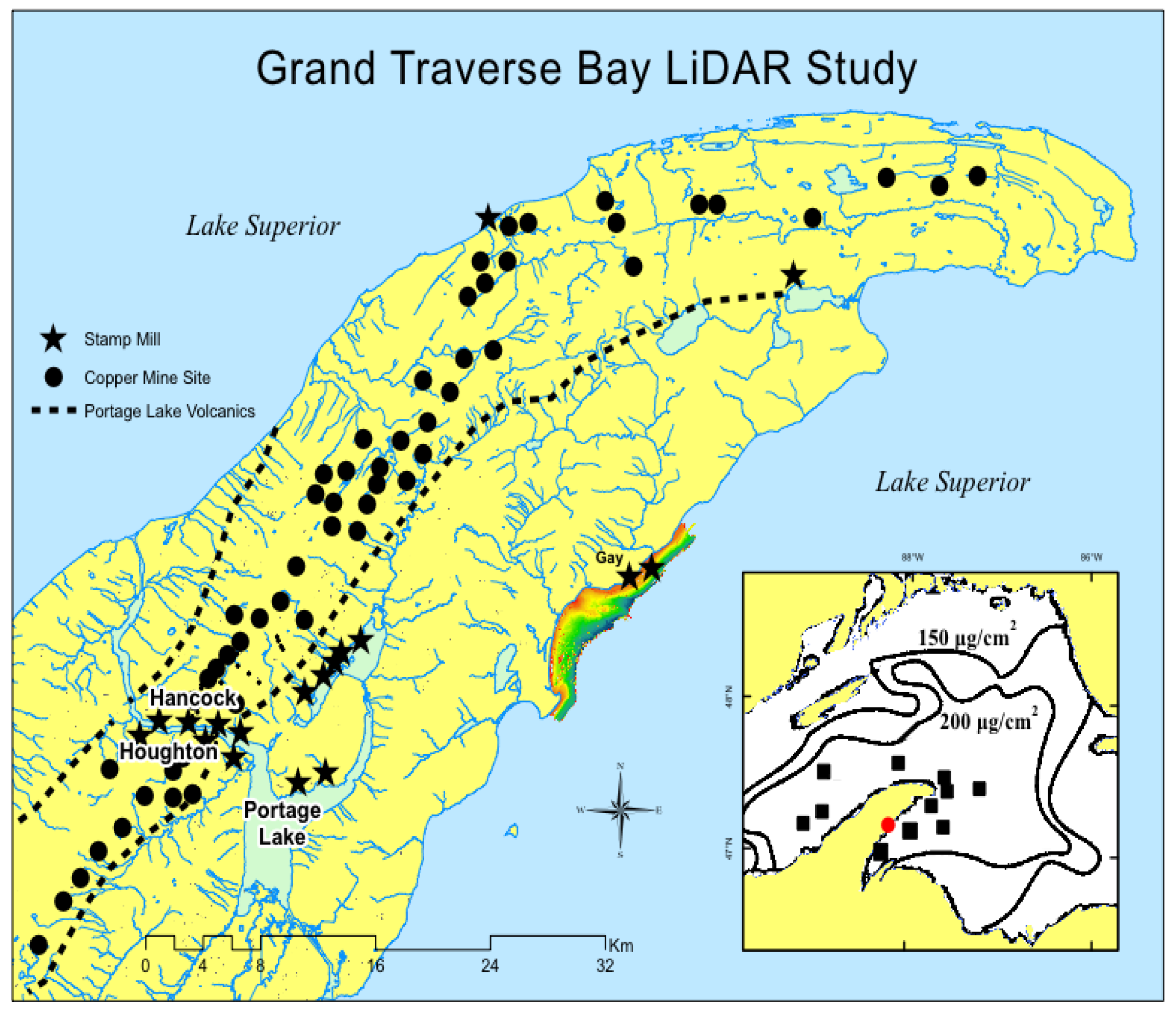
Figure 2.
Photos of the Gay Stamp Sand Pile. A) primary wooden discharge launder distributing tailings onto the Gay Pile, around 1922, with smaller sluices conveying stamp sand and slime clays laterally (courtesy MTU Archives). B) Photo of 6-8m high stamp sand bluffs on July 2008, showing a buried small lateral sluiceway protruding out of the pile along the shoreline. Lake Superior waters are to the right; the dark beach sands are stamp sands with slime clay layers. C) Bluff photo from about the same location in 2020, when shoreline erosion (ca. 7-8m/year) reached the buried primary launder wooden support beams, just before bluff removal. Concrete water launder is in background (B & C photos, courtesy W.C. Kerfoot).
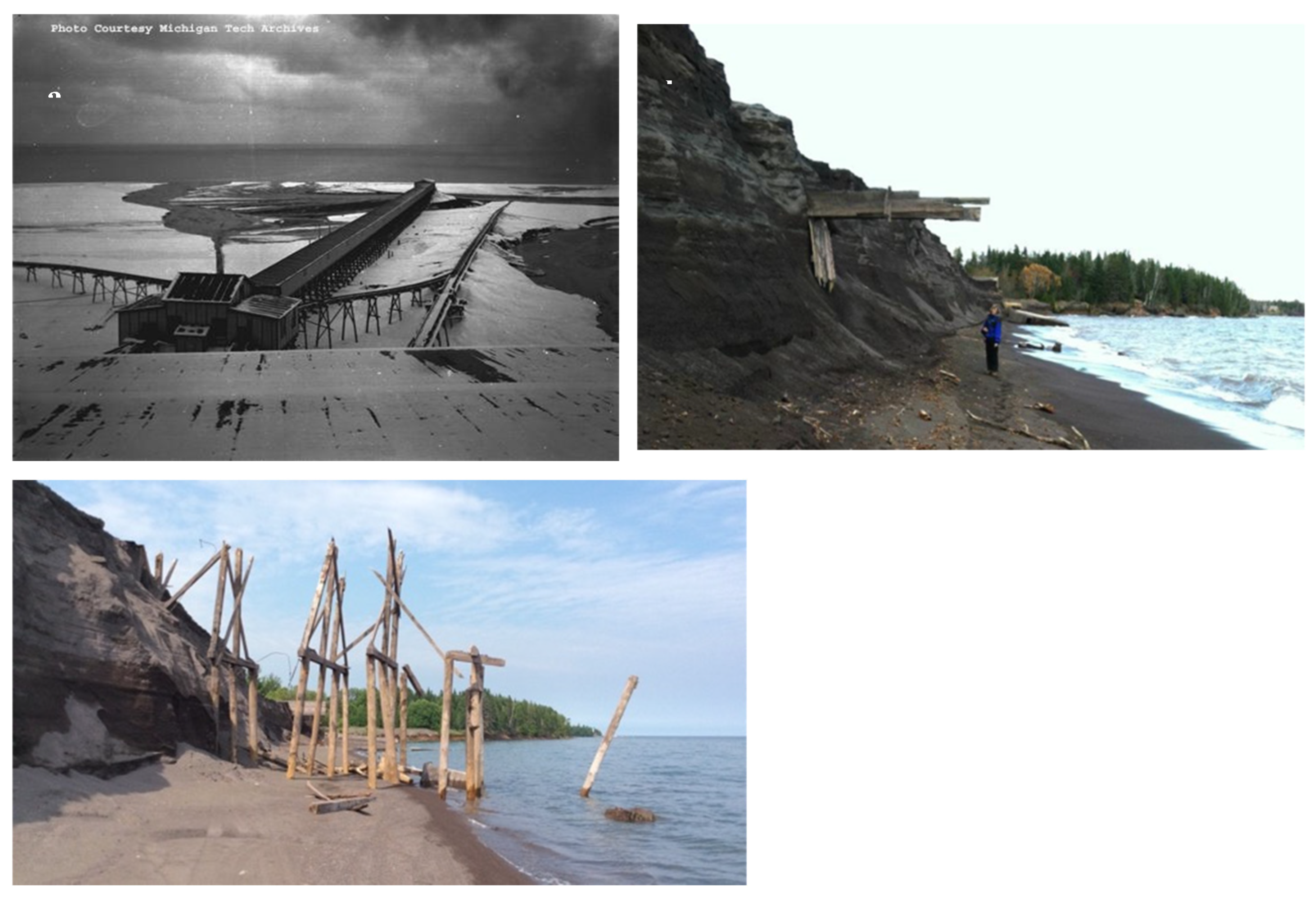
Figure 3.
Stamp Sands in situ under natural sunlight: a) wet redeposited stamp sand beach deposits close-up (12.5 cm wide field), showing colored crushed gangue mineral grains and b) from a distance, with a lens cap (6 cm) for scale, tailings appear as a dark, coarse-grained (2-4 mm), sand-sized beach deposit (photos courtesy Bob Regis).
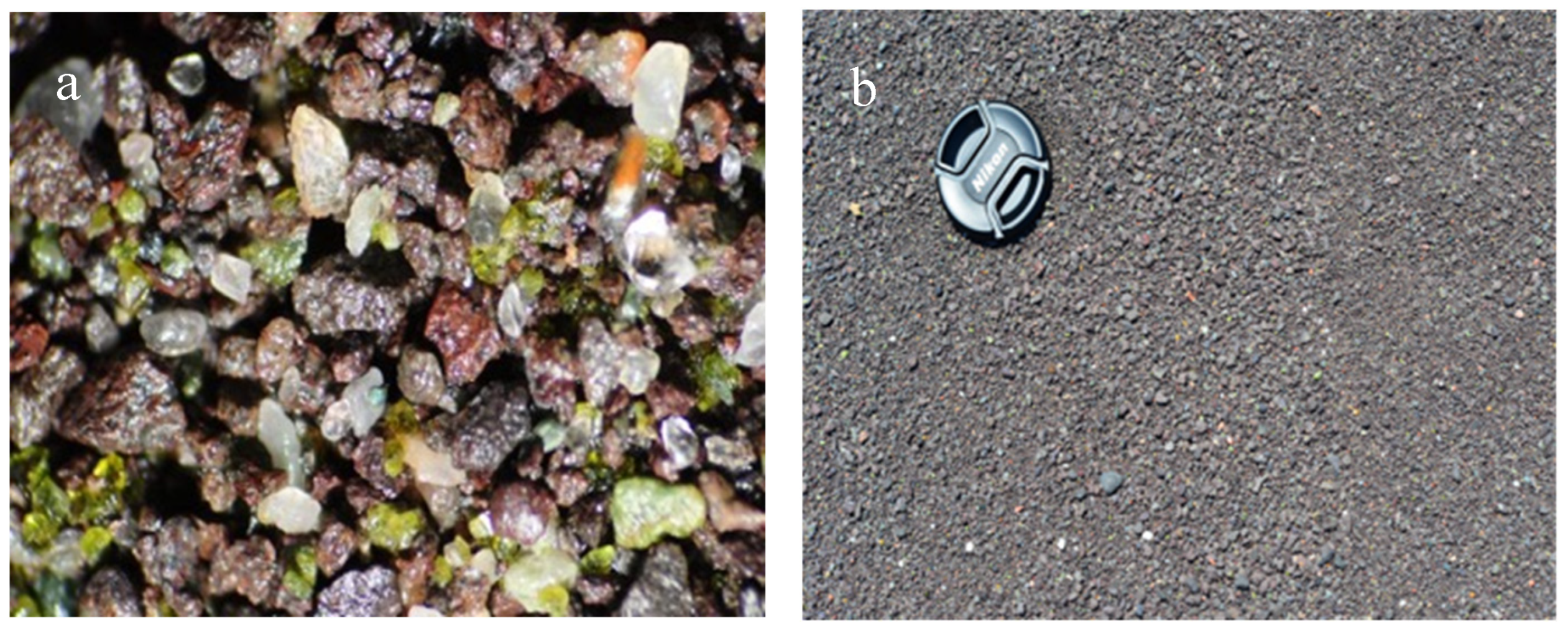
Figure 4.
Wolverine and Mohawk Mills at Gay, Michigan, around the late 1920’s to early 1930’s: (a) Railroad (Gay) frontside of mill complex, showing railroad station and where rails led up to the top floor of each mill. (b) Backside view of each mill. Steam driven stamps crushed the rock, and an assortment of jigs and tables used water on different floors to separate out denser copper-rich particles into concentrates shipped to smelters. The slime clay and stamp sand fractions were sluiced out onto a pile behind the two mills.
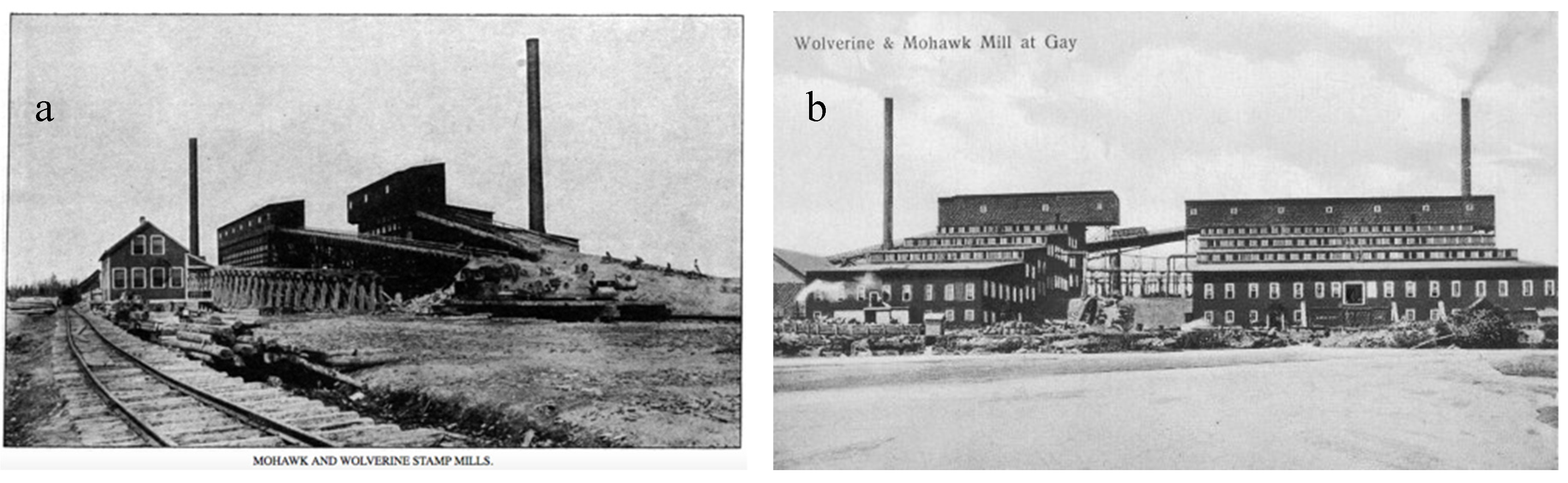
Figure 5.
(a) NOAA 2010 LiDAR DEM (digital elevation model) of Grand (Big) Traverse Bay, color-coded by elevation and water depth (depth scale to right). Red horizontal contour lines are at 5m depth intervals. Notice the position of the Gay tailings pile (“original pile”), migrating underwater stamp sand bars dropping into an ancient river channel (the “Trough”; at locations #1, and #5). On the eastern flanks of Buffalo Reef, stamp sands are moving out of the “Trough” into cobble/boulder fields (#3, #4). On the western edges, stamp sands have migrated as a beach deposit to the Traverse River Seawall (#8) and are slipping down into a depression (#7) next to cobble/boulder fields and moving around the harbor outlet. Hence, both the eastern and western edges of Buffalo Reef are experiencing stamp sand encroachment. Past the Traverse River, the sands in the southern bay are almost exclusively natural quartz grains (#9), forming a white beach with shoreline cusps and bar, plus ridges (#10) of natural sand moving from the shelf into deeper waters off the bay (modified from Kerfoot et al., 2014). (b) A 2016 LiDAR bathymetric DEM broken into dominant surface substrate types. Colored points indicate Ponar sampling sites and percentage of stamp sands across dominant surface substrate types (SS, stamp sand; NS, nature quartz sand; CBL cobble & boulders; BD, bedrock). A black dot indicates where the Ponar dredge was unable to capture a substrate sample, often bouncing off bedrock. Along the coastal margin, notice the scattered pond field, Coal Dock region, shoreline stamp sands, and Nipissing ridges. (c) Superimposed outline of Buffalo Reef boundaries with LiDAR-difference estimates (2008-2016) of erosion at Gay Pile shoreline (red) and deposition of underwater bars (blue) towards and into the “Trough”. One Tg (terragram) is equivalent to one million metric tonnes (MMT). This DEM aided planning for Stage 1 remediation (dredging of “Trough”). Buffalo Reef boundaries are indicated by thick black line.
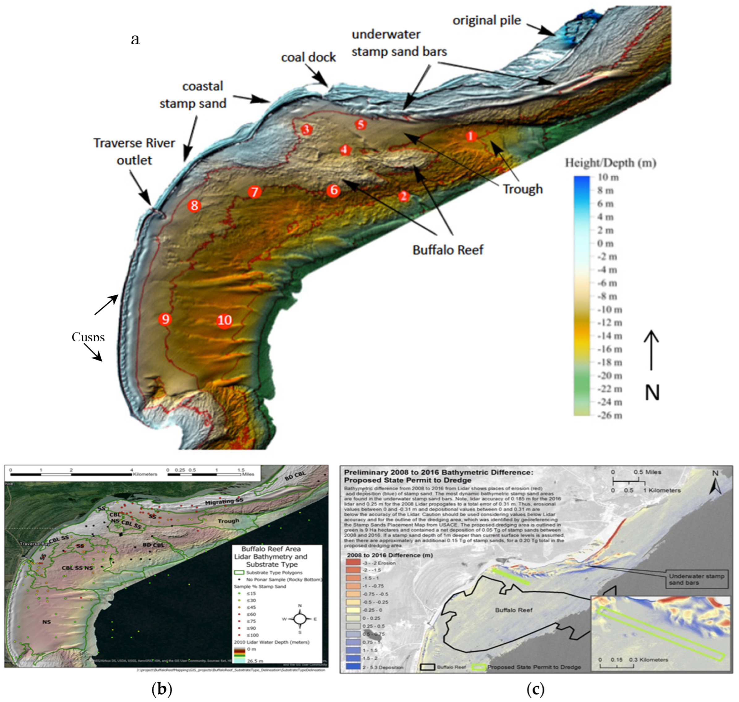
Figure 6.
For LiDAR, two laser pulses (blue-green 532 nm and near-IR 1064 nm) sweep across the lake surface: (a) The near-IR reflects off the water surface, whereas the blue-green penetrates through the water column and reflects off the lakebed. The difference between the two returning pulses gives the depth of the water column and details of bathymetry (modified from LeRocque and West [60]); (b) Simulated LiDAR waveform fitted with Gaussian function (water surface peak), a triangle function (water column reflectance), and a Weibull function for bottom reflectance (after Abdallah et al. [61]).
Figure 7.
Variety of low-cost UAS drone options used by MTRI: Images of Bergen Hexacopter, Quad-8, assorted small (sUAS) quadcopters (including Mariner, Splash2 waterproof), and a Micro Air Vehicle (MAV) quadcopter. Hand-held Micro-UAS quadcopter is in bottom left. The variety of field cases for the respective drones are shown in the next to bottom left, along with remote operations above a surface (far bottom right).
Figure 8.
a. Sample of sand grains from the Sand Point site in lower Traverse Bay (ca. 55% stamp sands) under transmitted light from a microscope, showing the contrast between rounded natural sand (transparent quartz) and dark sub-angular stamp sand grains (dark, irregular edges, slightly larger). Figure 8b. Size frequency distributions for the two particle types (stamp sand, red; natural quartz sand, blue) from the Sand Point site of Traverse Bay. Figure 8c. The grain counts (mixture of natural sand, stamp sand) follow a binomial distribution. The Coefficient of Variation (CV) for the %SS calculation is predicted from the equation under “Theoretical”. Field counts (see “Observed”, left) correspond generally to expected values. Over the interval from 10 to 90 %SS, the predicted CV (right) is between 15% to 2% (ca. mean of 5%).
Figure 9.
Daphnia pulex survivorship and fecundity experiment in stamp sand ponds at Gay. Forty 40mL vials had one adult Daphnia in each container and were submersed in shallow water of the ponds. Each vial had a 100µm mesh Nitex netting over the top, secured by rubber bands. A temperature probe was placed near the set to check daily temperature fluctuations during the experiment.
Figure 10.
UAS Seawall Drone Studies: A) Traverse River Harbor, showing stamp sand overtopping the Army Corps Seawall (2019). Notice highly stained (natural high DOC, low pH) water moving out of the river. The water depth descends sharply off the grey stamp sand beach on the right, whereas the natural white sand (quartz) beach on the left has a shallower nearshore draft and an offshore bar. Slight stamp sand lenses (dark) occur along the white sand beach margin. (photo, Colin Brooks, MTRI). B) Initial drone UAS Orthomosaic Survey (upper right, Hunter King, MI EGLE) from late 2019. MTRI 2019 Digital Elevation Model (DEM; colored, hillshaded, left), contoured from GPS Ellipsoidal Height; elevation profiles along cross-section transect lines (1-5, bottom right). Contouring emphasizes the increased width and vertical height of stamp sand accumulating against the Seawall (Colin Brooks, MTRI).
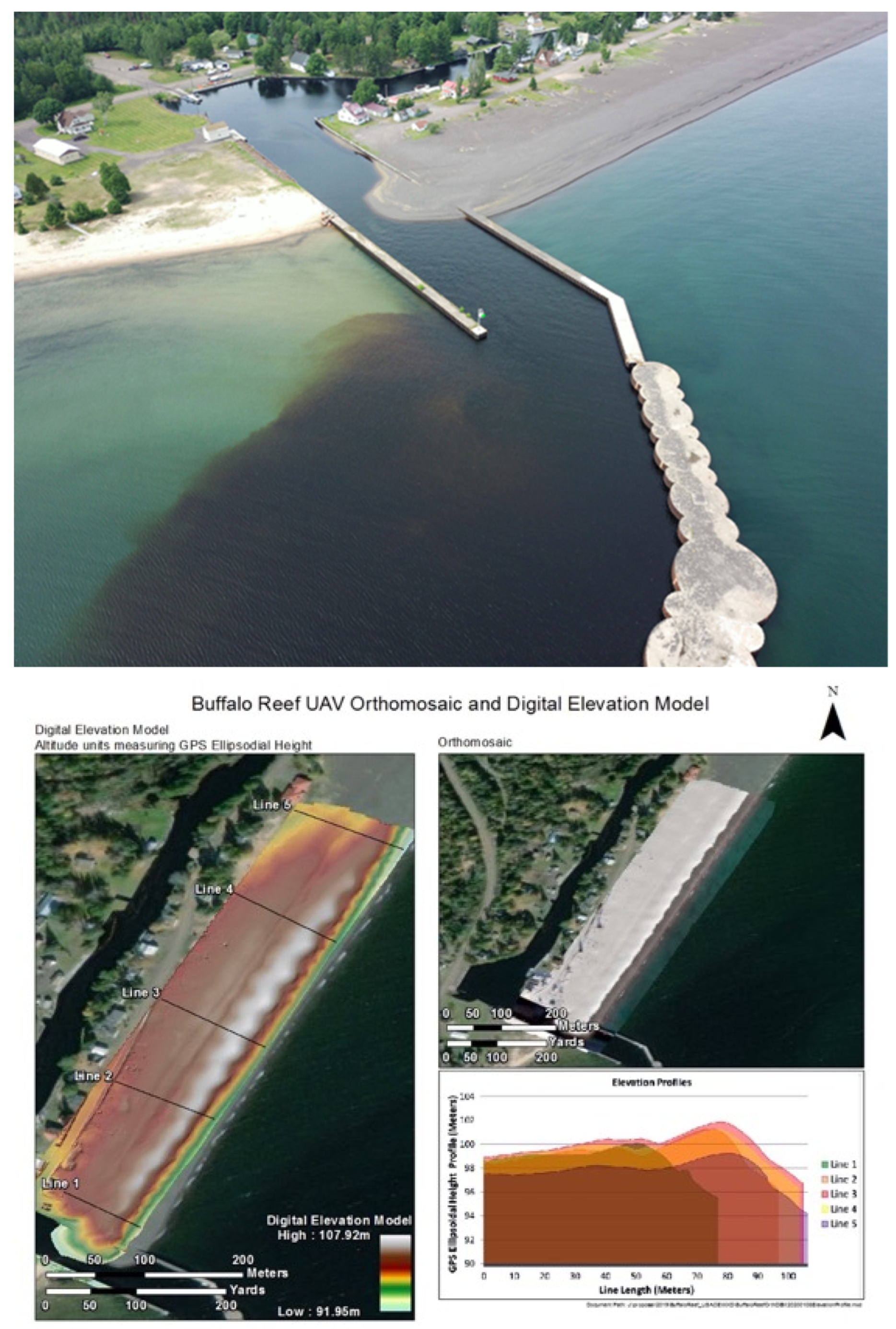
Figure 11.
Army Corps initial remediation plans and implementation steps (dredging & berm placement): a) Army Corps planned dredging of stamp sand from the Traverse River Harbor (2017-21) and “Trough” (2020-21) and deposition into a “Berm Complex”. b) initial dredging begins at the Traverse River Harbor (fall of 2017); c) 5-7 km of pipes and pumping stations used to transport stamp sand from the Traverse Harbor and “Trough” to the “Berm Complex” (2019-2021). (map courtesy of Army Corps, Detroit; photos courtesy W.C. Kerfoot).
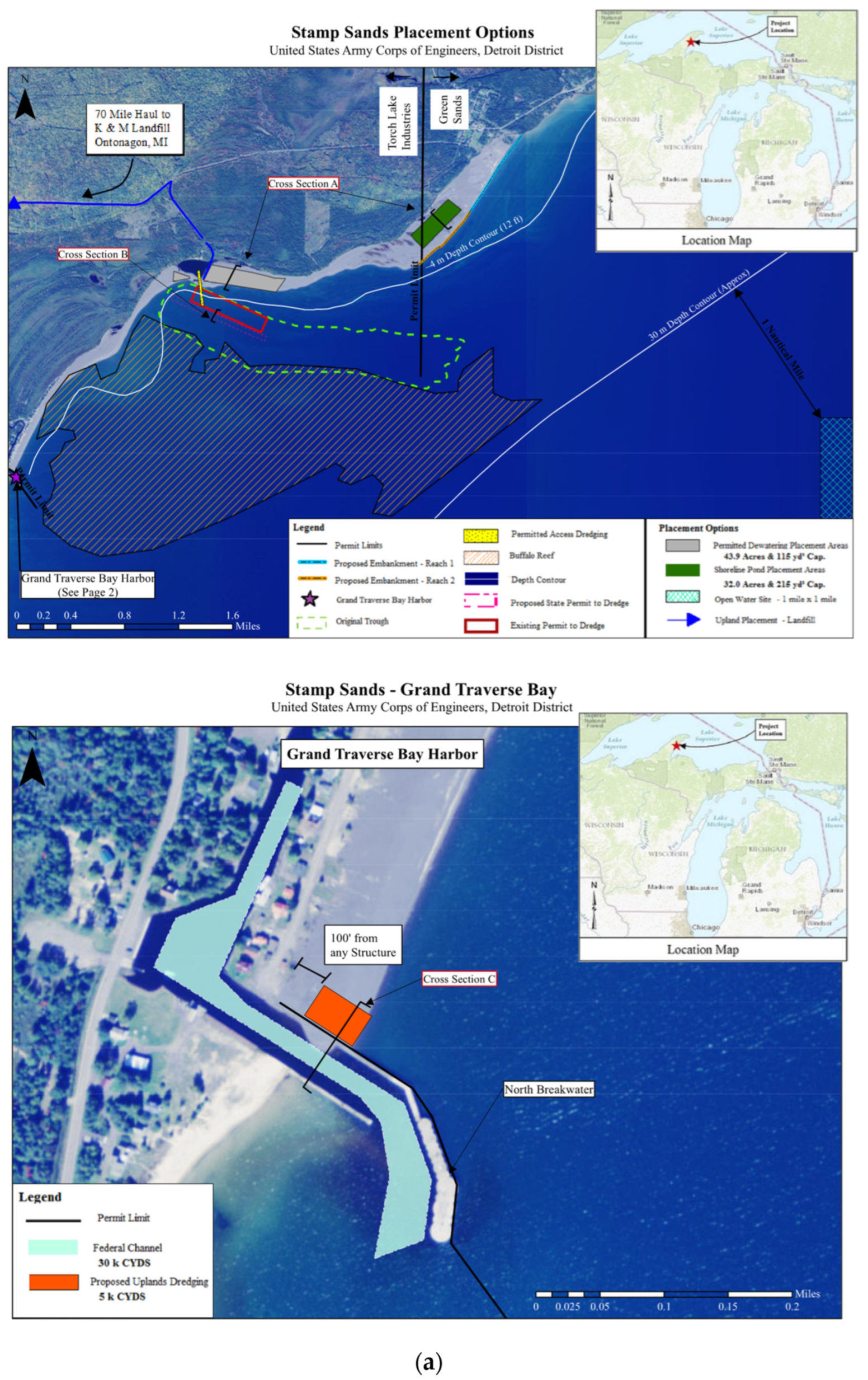
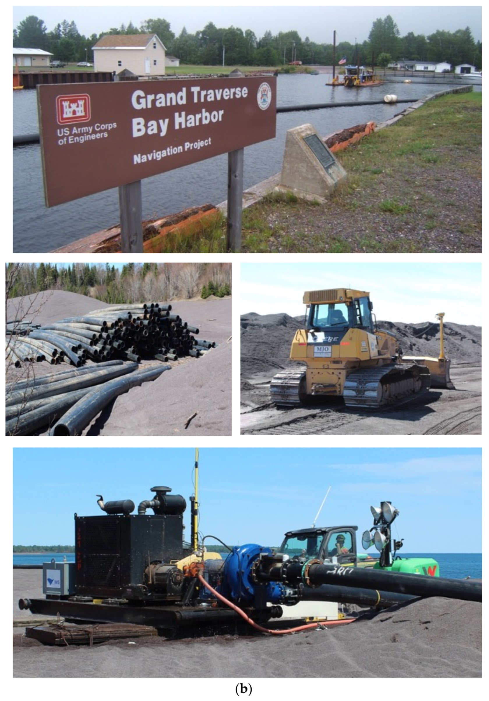
Disclaimer/Publisher’s Note: The statements, opinions and data contained in all publications are solely those of the individual author(s) and contributor(s) and not of MDPI and/or the editor(s). MDPI and/or the editor(s) disclaim responsibility for any injury to people or property resulting from any ideas, methods, instructions or products referred to in the content. |
© 2024 by the authors. Licensee MDPI, Basel, Switzerland. This article is an open access article distributed under the terms and conditions of the Creative Commons Attribution (CC BY) license (https://creativecommons.org/licenses/by/4.0/).
Copyright: This open access article is published under a Creative Commons CC BY 4.0 license, which permit the free download, distribution, and reuse, provided that the author and preprint are cited in any reuse.


