
Submitted:
11 April 2024
Posted:
12 April 2024
You are already at the latest version
Abstract
Air quality is a topic of growing relevance on the global agenda. Two key indicators of air quali-ty, nitrogen dioxide (NO2) and carbon monoxide (CO), represent significant hazards to human health and the environment putting the sustainability of natural resources at risk. Therefore, it is imperative to regularly monitor and reduce atmospheric pollutant concentrations to mitigate their harmful consequences. This study presents an analysis of NO2 total and CO emissions in Argentina, utilizing remote sensing data. The research aims to determine the spatiotemporal distribution of NO2 and CO emissions in Argentina from 2019 to 2021. Subsequently, it seeks to establish the influence of land uses and land cover on the emission of NO2 and CO through dif-ferent climatic, anthropic, and natural indicators. The study was carried out in Argentina during the period 2019-2021, where random points were placed for the different land covers with a total of 800 points surveyed. The year with the highest CO concentration (mol/m-2) was 2020. The values were highest for tree covers and herbaceous wetland coverage in the northern part of the country. For total NO2, the highest concentrations were reached during the years 2020 and 2021. Regarding its distribution, throughout the evaluated period, the highest concentrations of total NO2 were found in the built-up and cropland coverages, with the capital of the country and the northern region of the Buenos Aires province being the most affected areas. In addition, the concentration of CO was influenced by climatic variables (atmospheric pressure, wind speed, maximum environment temperature, Palmer index), natural (height, humidity, NDVI), and ur-ban variables (distances to mining extraction, airports, power plants, urban index) for the differ-ent uses and land covers. Finally, the concentrations of total NO2 were influenced by climatic variables (Palmer index and wind speed), natural (height and NDVI), and urban variables (dis-tance to airports, power plants, industries, service stations, and open dumpsites) for the differ-ent uses and land cover. This study contributes to sustainable environmental management, ena-bling the formulation of effective strategies for mitigating emissions and promoting the long-term health and well-being of communities.
Keywords:
atmospheric pollution
; remote sensing data
; land uses and land cover
; gases
; environmental management
1. Introduction
Air quality is an increasingly relevant issue on the global agenda, supported by recognition in the United Nations Sustainable Development Goals (SDGs). These goals, addressing health, energy, and sustainable urban development, are linked to the issue of air pollution [1]. Air pollution is considered the world's greatest environmental health threat, causing 7 million deaths worldwide each year [2]. Exposure to air pollutants is the most critical risk factor for major non-communicable diseases [3]. In a context where air quality has become a critical factor for public health, it is alarming to note that outdoor air pollution contributed to 4.2 million deaths worldwide in 2016, according to the World Health Organization [4]. These staggering figures reveal that air pollution is a global challenge deeply affecting human health. WHO assessment indicates that this pollution is responsible for 29% of lung cancer deaths, 43% of chronic obstructive pulmonary disease (COPD) deaths, approximately 25% of deaths from ischemic heart disease, and 24% of deaths from strokes globally [5].
This environmental issue knows no borders, and Argentina is no exception. Air pollution in the country is a topic deserving increasing attention. Its main causes are diverse, ranging from economic development and urbanization to energy consumption, transportation, and rapid urban population growth [6]. Two key indicators of air quality, nitrogen dioxide (NO2) and carbon monoxide (CO), pose significant hazards to human health and the environment [7]. Therefore, it is imperative to periodically monitor and reduce atmospheric pollutant concentrations to mitigate their harmful consequences.
Nitrogen oxide (NO2) plays a crucial role in atmospheric chemistry, air quality, and climate change, acting as indirect greenhouse gases contributing to global warming [8]. These NO2 originate from both natural sources and human activity, with fossil fuel combustion being the predominant source. Their presence in urban areas, where multiple emission sources and dense populations are concentrated, further exacerbates health risks. Meanwhile, carbon monoxide (CO), another critical pollutant, is primarily released through incomplete combustion of fossil fuels and industrial processes, making it a significant concern for public health [9]. Forest fires are a source of many air pollutants in the atmosphere. During such events, significant amounts of carbon monoxide (CO), nitrogen oxides such as NO, NO2, methane (CH4), and non-methane hydrocarbons (NMHC) are released. Their emissions significantly disrupt chemical climate on local, regional, and global scales [10]. They chemically produce ozone, a secondary pollutant, which is an oxidizing agent and a greenhouse gas with potential climate implications [10].
Land use and land cover change (LULCC) are fundamental factors influencing environmental dynamics and atmospheric emissions worldwide [11]. Land cover refers to the surface class covering the land, such as forests, grasslands, urban areas, etc., while land use refers to how the land is used, such as agriculture, urbanization, industry, etc. Land use/cover change (LULCC) has become one of the key elements in global environmental change and sustainable development [12]. This is due to its omnipresence at the local scale and its globally recognized environmental impact [11]. The intensification of agricultural and industrial activities driven by rapid population growth has led to significant changes in LULC (Land Use Land Cover) and increased demands on natural resources housed in the land [11]. In Argentina, a country known for its diverse ecosystems and extensive agricultural landscapes, understanding the intricate relationship between land use patterns and emissions of nitrogen oxides (NO2) and carbon monoxide (CO) is crucial for sustainable environmental management.
As noted by Le et al. [13], the intricate interaction between land use changes and atmospheric emissions requires a multi-temporal analysis to unravel the dynamics shaping environmental impacts. This aspect resonates with the urgent need for comprehensive assessments, as echoed by Ooi et al. [14], to effectively mitigate the consequences of land use alterations on air quality and atmospheric composition. Despite the importance of understanding and monitoring these trace gases, research on NO2 and CO in the region of South America is limited, adding to the lack of air quality monitoring stations in many Latin American countries. However, in recent decades, the availability of satellite observations, such as the Tropospheric Monitoring Instrument (TROPOMI) aboard the Copernicus Sentinel-5 Precursor (S5P) satellite, has allowed unprecedented access to NO2 and CO measurements with global spatial coverage [15].
In this context, this study aims to delve into the multi-temporal dynamics of NO2 and CO emissions in Argentina, driven by changes in land use and cover. Through a robust methodology integrating remote sensing techniques and atmospheric modeling. Insights gained from this analysis will not only improve our understanding of spatiotemporal emission patterns but also provide invaluable guidance for sustainable environmental management practices. Through a multi-temporal analysis, it seeks to elucidate the underlying processes driving environmental changes, thus fostering sustainable management strategies for the preservation of Argentina's ecosystems and atmospheric quality. The main objective of this work is to identify and analyze the spatial distribution and behavioral patterns of these two trace gases, CO and NO2, in Argentina, using data collected over 3 years (2019-2021) and determine the spatial impact factors on land use/cover (LULC) in the emission of these gases through different climatic, anthropogenic, and natural indicators. Despite the short duration of this period, possible trends will be explored to shed light on the evolution of these pollutants in the region. This study is essential for better understanding environmental risks and health associated with air quality in Argentina and may lay the groundwork for future policies and mitigation measures.
2. Materials and Methods
2.1. Study Area
Argentina occupies the southern tip of South America between parallels 22 and 56 south, with wide access to the Atlantic Sea. The study area is composed of 23 provinces and the Autonomous City of Buenos Aires, the capital of the country, with a total area of 2,780,400 km² (Figure 1). It is the second-largest country in South America and the eighth-largest in the world. The climate of Argentina is determined by its latitudinal extension, encompassing warm subtropical climates in the north, temperate climates in the central east, arid climates that cross the country from north to south, and cold climates in the south [https://www.ign.gob.ar/]. Its relief is predominantly plain except in the west of the country, along the Andes Mountain range where the highest altitudes in America are reached (Aconcagua 6,960 meters). The country's population, according to the preliminary result of the 2022 census, is 45,892,285 habitants (https://censo.gob.ar/index.php/datos_definitivos_total_pais/). In Argentina, the primary sources of atmospheric pollution are energy (50.7%), agriculture, livestock, forestry, and other land uses (39.1%), industrial processes and product use (5.7%), and waste (4.5%). Housing contributes an average of 29% of emissions. CO2 emissions in 2021 reached 366 megatons, ranking Argentina as the 155th country in terms of CO2 emissions [https://www.argentina.gob.ar/sites/default/files/iea2021_digital.pdf].
2.2. Data and Preprocessing
In this study, various spatial data from satellite remote sensing as well as from existing geospatial data were used. In particular, these include air quality data and data that describe natural, climatic, and urban indicators. Due to the input data having different resolutions, 1 km was chosen as the uniform spatial unit. In addition, 100 random polygons were taken for each land use and cover for the years 2019, 2020, and 2021. The centroid of the polygon was then extracted and a total of 800 points per year were obtained. Furthermore, the area occupied by each polygon was extracted. The methodological flow is illustrated in Figure 2. The LULC maps were obtained from the European Space Agency (ESA) World Cover based on Sentinel-1 and Sentinel-2 data for the years 2019-2021. The land cover classes selected were:
- Tree cover: This class includes any geographic area dominated by trees with a cover of 10% or more.
- Shrubland: This class includes any geographic area dominated by natural shrubs having a cover of 10% or more.
- Grassland: This class includes any geographic area dominated by natural herbaceous plants (Plants without persistent stems or shoots above ground and lacking definite firm structure): (grasslands, prairies, steppes, savannahs, pastures) with a cover of 10% or more.
- Cropland: Land covered with annual cropland that is sowed/planted and harvestable at least once within the 12 months after the sowing/planting date.
- Built-up: Land covered by buildings, roads, and other man-made structures such as railroads. Buildings include both residential and industrial buildings. Urban green (parks, sports facilities) is not included in this class. Waste dump deposits and extraction sites are considered bare.
- Bare/sparse vegetation: Land with exposed soil, sand, or rocks and never has more than 10 % vegetated cover during any time of the year.
- Permanent water bodies: This class includes any geographic area covered for most of the year (more than 9 months) by water bodies: lakes, reservoirs, and rivers. Can be either fresh or salt-water bodies. In some cases, the water can be frozen for part of the year (less than 9 months).
- Herbaceous wetland: Land dominated by natural herbaceous vegetation (cover of 10% or more) that is permanently or regularly flooded by fresh, brackish, or salt water.
2.2.1. TROPOMI Product
In the first step of the study, the product Offline stream of the NO2 total column and the CO column from satellite TROPOMI (Tropospheric Monitoring Instrument) was used to extract the median annual NO2 and CO emissions, for the period from January 2019 to December 2021. The spatial resolution of the image is 1113.2 meters. Using Engine Code Editor, pollution parameter maps (CO and NO2) were extracted. Using filters, the study years and the location (country Argentina) were defined. Following that, images with clouds were filtered by defining cloud filters and median filters. The data was downloaded and processed using the QGIS software.
2.2.2. Anthropic indicators
El UI (Urban Index) is an indicator of built-up areas [16] and was obtained using the following equation (Equation 1):
the UI highlights urban areas with higher reflectance in the shortwave-infrared (SWIR2) region, compared to the Near Infra-red (NIR) region. The BI value ranges from -1 to +1. Values close to 1 indicate a high density of built-up areas.
UI = SWIR2 (Band12) - NIR(Band8a)/ SWIR2 (Band12) + NIR (Band8a),
To extract the following variables, the minimum distance from the centroid of each polygon to the following vector layers was taken: Mining extraction, Power plants, Airports, Open dumpsites, Service stations, Factories-Industry, and National routes. The layers were downloaded from the National Geographic Institute of the Argentine Republic [https://www.ign.gob.ar/NuestrasActividades/InformacionGeoespacial/CapasSIG].
2.2.3. Climatic Indicators
The climatic variables were extracted from TerraClimate. This is a high spatial resolution global gridded climate dataset that provides monthly values for a wide range of climate variables [17]. The annual average was extracted from the following variables:
- Palmer Drought Index: The index uses precipitation and environment temperature data to study moisture supply and demand using a simple water balance model. Negative values indicate droughts and positive values indicate wet areas.
- Vapor pressure (kPa)
- Max and Min environment temperature (°C)
- Wind speed (m/s)
2.2.4. Natural indicators
The NDVI and Tasseled Cap variables were extracted using Sentinel-2 imagery. These were processed by applying a filter and mask of clouds less than 10%. Then, the median values for each year were extracted.
- NDVI (normalized vegetation index.): NDVI is based on the reflectance of the NIR wave in healthy plants and on the reflectance of the red wave to detect less healthy plants. This index is defined by values ranging from -1 to 1.
NDVI = NIR (Band 8) - RED (Band 4) / NIR (Band 8) + RED (Band 4)
- Tasseled Cap:
- Brightness: low brightness values in coincidence with forested areas or, in general, with vegetation cover or bodies of water;
Brightness = (B2*0.3029) + (B3*0.2786) + (B4*0.4733) + (B8*0.5599) + (B11*0.508) + (B12*0.1872)
- 2.
- Greenness: it is related to plant masses and bodies of water;
Greenness = (B2*-0.2941) + (B3*-0.243) + (B4*-0.5424) + (B8*0.7276) + (B11*0.0713) + (B12*-0.1608)
- 3.
- Humidity: related mainly to bodies of water, but also the moisture content of vegetation and soils;
Humidity = (B2*0.1511) + (B3*0.1973) + (B4*0.3283) + (B8*0.3407) + (B11*-0.7117) + (B12*-0.4559)
- 4.
- DEM: This SRTM V3 product (SRTM Plus) is provided by NASA JPL at a resolution of 1 arc-second (approximately 30 m).
2.3. Statistical Analysis
Descriptive statistics for the spatiotemporal distribution of CO and NO2 gases were performed. Additionally, GLM (Generalized Linear Models) with gamma distribution between the gases and the interaction between the different LULC coverage and the area of each sampled polygon were made. Spatial autocorrelation between polygons was evaluated through the nearest neighbor method. Then, the variance inflation factor (VIFs) for any remaining collinearity on the full models from different sets and excluded variables with VIFs > 5 was assessed, which indicates collinearity between predictors [18]. For objective 2, generalized linear models with Gamma distribution only for the data from the year 2021 were performed. Some cover classes were regrouped because they presented similar values in CO and NO2 concentrations: tree cover-herbaceous wetland, shrubland-grassland, and cropland-built-up. The Permanent water bodies class was explained from the models. The CO and NO2 concentrations were related to different predictor variables classified as anthropic, climatic, and natural (see section 2.2.). For each full model, a backward elimination procedure was used to remove no significant variables without losing important information (significance level p-value > 0.05 can be eliminated) and to obtain the minimal adequate model [19] A pseudo-R2 was estimated from the deviance values of the best models [20]. To identify collinearity between independent variables, the Pearson correlation method was used [21]. When the coefficient r was > |0.7|, variables were excluded.
3. Results and Discussion
This section may be divided by subheadings. It should provide a concise and precise description of the experimental results, their interpretation, as well as the experimental conclusions that can be drawn.
3.1. Spatiotemporal Distribution of CO and NO2 in Argentina during the Years 2019, 2020, and 2021
The results of the spatiotemporal distribution of CO and NO2 in Argentina are presented in Figure 3 and Figure 4 annually. According to Figure 3, the CO concentration presented its highest values for the year 2020 (max-value = 2.99x10⁻² mol/m-2), obtaining similar values for the years 2019 and 2021 (max-value = 2.17×10⁻², max-value = 2.09×10⁻² mol/m-2 respectively). These results differ from those found in other countries since several authors claim that CO emissions decreased during the 2020 confinement due to the COVID-19 pandemic [ 22, 23, 24]. Although the pandemic may have had a significant impact on some human activities and therefore CO emissions, other factors could have influenced CO emissions during that period. One of the possible reasons could be due to changes in industrial activity. That is to say, even though the pandemic reduced most activities (industrial and commercial), some essential product industries continued to operate normally or even increased their production due to the strong demand for certain products. Another explanation could be due to changes in transportation patterns, although vehicle traffic was reduced due to the confinement measures. Some sectors, such as the transportation of food and essential goods increased their activity, which could have offset the reductions in other sectors. In summary, it is important to consider several factors when analyzing carbon monoxide (CO) emissions in a country over a specific period, such as the impact of the COVID-19 pandemic on emissions. While the COVID-19 pandemic could have had a significant impact on some activities and therefore CO emissions, there are also other factors to consider when analyzing total CO emissions over a specific period. A comprehensive analysis that takes all of these factors into account is essential to fully understand CO emissions trends in a country over a given period.
Regarding the spatial distribution of CO, the highest values were found in northeastern Argentina, coinciding with the areas of greatest vegetation cover such as the phytogeographic province Parque Chaqueño and with a high number of fires per year (Figure 3). Although southern Argentina also has forest cover such as the Andean-Patagonic forests, fires are less frequent [25, 26]. Furthermore, the high CO concentrations in northern Argentina could be due to warm and humid climatic conditions compared to those in the south. These conditions favor the decomposition of organic matter and bacterial activity, which could result in greater release of CO in forests. Finally, human activity such as agriculture, livestock, industrial, and vehicular traffic is more intense in the north of Argentina because it has a higher population density, which contributes to higher levels of CO in the air [ 27].
Regarding NO2 concentrations, the maximum values recorded increased from 2019 to 2021 (max-value = 3.72×10⁻², 7.74×10⁻², and 8.13×10⁻² mmol/m-2 respectively). Figure 4 shows that the highest concentrations were found in the urban areas of Argentina. According to Gallardo et al., [9], NO2 emissions are associated with high environment temperature and high oxygen content processes and occur mainly in the form of NO. In high-traffic urban areas, diesel vehicles can produce a significant contribution of NO2. Also, the model showed a relationship between the NO2 concentration and the interaction between explanatory variables area of the polygons and the class built-up land cover (Estimate = 5.826×10⁻⁶, p-value < 0.001), where the concentration of NO2 begins to be significant from an area greater than 6000 hectares for the urban class (Figure 5). This is the first work that demonstrates the minimum size of the urban area where NO2 concentrations begin to be significant for the environment. The models with CO concentrations and the interaction between area and LULC did not show significant differences. This indicates that CO concentrations tend to remain in lower altitude areas of Argentina regions, such as valleys in mountainous areas or cities or natural areas close to sea level.
3.2. Influence of Land Uses and Land Cover on the Emission of CO and NO2 over Time through Different Anthropic, Climatic, and Natural Indicator
GLMs were carried out to identify different anthropic, climatic, and natural indicators that affect the concentrations of CO and NO2 in distinct LULC. Due to some uses and land covers having similar behavior in terms of the concentrations of these gases, the classes tree cover and herbaceous wetland, shrublands, grasslands, cropland, and built-up were grouped. The class bare/sparse vegetation was not grouped.
3.2.1. CO
In general, the variable distance from the mining extraction affected the CO concentrations independently of the type of land cover (Table 1), where the CO concentration increased as the distance to the mining extractions was smaller. This increase near mining companies is because the majority belong to crude oil extractions, which release volatile organic compounds in the process such as CO, CO2, carbonic acid, ammonium carbonate, and carbonates. Oil production, exploration/extraction sites, and refineries are the second largest sources of volatile compounds after vehicle exhaust gases in the transportation sector [28] This is because volatile compounds can escape from the oil mass during all stages of the crude oil industry [29].
The variable distance to the routes influenced the coverage of tree cover-herbaceous wetland and cropland built-up, where it could be observed that CO increased as the distance to the main routes decreased (Table 1). These results were expected in cropland-built-up coverage where human activity is more intense [30]. However, the tree cover-herbaceous wetlands were also affected by the distances to the routes concerning CO concentrations increasing as the distance to the routes decreased. This could be explained because the routes with the highest values of annual vehicular traffic are located in the northwest of the country, coinciding with the coverage of tree-cover-herbaceous wetlands (https://www.argentina.gob.ar/obras-publicas/vialidad-nacional/sig-vial). Although sites with high vegetation cover are the main sinks of CO, probably when vehicular traffic is very intense, the vegetation cannot efficiently capture the CO emitted by the combustion of vehicles. [31]. Additionally, the decomposition of organic matter, such as leaf litter and dead wood, can release CO as a byproduct of bacterial decomposition. In herbaceous wetlands, the anaerobic decomposition process of organic matter can also generate CO as a waste product. Microorganisms present in the swamp soil decompose organic matter under conditions of low oxygen availability, leading to the release of CO. In summary, in both forests and herbaceous wetlands, the decomposition of organic matter is an important source of CO, which can result in higher concentrations of this gas in the air [32]. While forests can also have CO emissions due to the decomposition of organic matter, these levels tend to be lower compared to anthropogenic emissions in cities [33].
The distance to power plants and airports had a negative influence on Shrubland-Grassland coverage since CO concentrations increased when the distance was smaller. Although shrubs and grasslands capture a CO percentage from the environment, power stations, and airports generate a greater amount of CO released to the environment than these covers can sequester. In cropland-built-up coverage, CO concentrations also increased as the distance to airports decreased. These results coincide with studies carried out at airports, which showed slightly elevated CO, NO2, and SO2 concentrations [34]. Hudda et al. [35] show the impact of aviation on surrounding residential areas where the highest CO concentrations were around airports up to 12 km. In the present study, CO concentrations were recorded in a range of 2 to 300 km from the nearest airports. Finally, the urban index measured in the different land covers influenced only the bare/sparse vegetation soil cover, where the CO concentrations increase, the urban index also increases, reaching values close to 1. These results are in line with what was expected since within this category are waste dump deposits and extraction sites, which take values close to 1 within the index range. Most of the garbage dumps in Argentina are open dumpsites, some illegal and uncontrolled “landfills”. Siddiqua et al. [36] found that landfilling is associated with various environmental pollution, including air pollution due to the emissions of gases, which could cause illnesses in the exposed population living in their vicinity. Furthermore, the decomposition of organic materials in landfills produces different gases that have a composition of 50% of CH4, 50% of CO2, and a small amount of non-methane organic compounds [37, 38]. Mining wastes and the difficulty of removal are very often sent for recovery or neutralization, whereas neutralization most often means disposal in dedicated landfills [39].
On the other hand, the results showed that CO concentration increased with the maximum environment temperature, wind speed, and vapor pressure in multiple land cover types. (Table 1). As expected, high CO emissions into the atmosphere increase the environmental temperature, especially in cropland and built-up areas [40]. In natural areas such as tree cover, herbaceous wetlands, shrublands, and grasslands, CO emissions also increased along with the environmental temperature. However, the Palmer index presents a negative relationship with the cover of the tree cover and herbaceous wetland. This indicates that in extremely dry forests the concentration of CO is greater. The increase in the environmental temperature, together with conditions of extreme drought, leads to a greater predisposition to forest fires and consequently a greater emission of CO into the atmosphere. Finally, the CO concentrations presented a direct relationship with the rate of the winds in the different coverages. This indicates that CO concentrations move through the atmosphere with the rate and direction of the winds. The natural variable, height (DEM) negatively affected CO concentrations for shrubland and grasslands, cropland and built-up areas, and bare/sparse vegetation covers (Table 1). That is to say, CO concentrations increase with the altitude decrease, indicating that CO concentrations tend to remain in lower altitudes of Argentina areas, such as valleys in mountainous areas, cities, or natural areas close to sea level. However, a study in China showed simulation models that reported that as urban land expands, the atmospheric load of CO and PM2.5 decreases near the surface (below km), but increases at higher altitudes (1 to 4 km) [41]. The humidity variable determined from the Tasseled Cap also negatively affected CO concentrations but only in shrubland and grassland covers. This indicates that the lower the humidity of the bush and grassland vegetation, the greater the CO concentration. Finally, the variable NDVI negatively affected CO concentrations for cropland and built-up areas. NDVI is an important phase indicator of terrestrial photosynthesis, which is usually used to analyze the CO2 variation caused by vegetation [42]. Low NDVI values indicate areas with low coverage or impermeable surfaces such as cities, while values close to 1 indicate areas with vegetation such as cultivated areas. This work shows a gradual decrease in CO concentrations from urban to cultivated areas of the country.
3.2.2. NO2
Accepted that NO2 is not only a greenhouse gas but also contributes to ozone depletion in the stratosphere. However, it is much more reactive than CO2 and therefore promotes combustion. NO2 has an average residence time in the atmosphere of 170 years. At the current production rate, it is estimated that NO2 concentrations will reach approximately 375 ppb per year.
In general, the urban variables that negatively affected the concentration of total NO2 were open dumpsites, distance to power plants, service stations, airports, and factories-industry for the different LULC. This indicates that the shorter the distance to the different urban variables, the higher the total NO2 concentration (Table 2). The distance to the service stations harmed natural areas such as tree cover-herbaceous wetland and shrubland-grassland coverage.
This indicates that NO2 concentrations increased with the distance to gas stations decrease (Table 2). This finding is supported by previous studies that have shown that NO2 emissions, mainly derived from vehicular traffic, can significantly increase in areas near gas stations [43]. Gas stations act as fuel refilling points and therefore attract a high volume of vehicular traffic. Previous studies have demonstrated that NO2 emissions associated with traffic near service stations can contribute significantly to air pollution in urban and service stations [44]. Furthermore, NO2 emissions may be more pronounced in areas near gas stations due to the higher number of vehicles that are in the process of stopping or accelerating when entering or leaving these facilities [45]. There is some concern about the different nitrogen oxides such as NO2, N2O, and NO released into the atmosphere by automobiles and other mobile sources. [46]. In addition, this work demonstrated that the natural areas sampled did not reduce NO2 concentrations around the service stations.
The covers of trees, herbaceous wetlands, and cropland built-up, presented an inverse relationship between NO2 concentrations and distances to power plants. According to Puliafito et al. [47] air quality pollutants, such as NO2 and SO2, are mainly emitted by the transportation and energy sector. This is supported by previous research that has shown that NO2 emissions from power plants can contribute significantly to local air pollution [48, 49]. Power plants often burn coal, natural gas, or other fossil fuels to generate electricity, resulting in the release of air pollutants, including NO2, as a byproduct of combustion [50]. Also, it was found that proximity to airports also had a negative effect on tree cover-herbaceous wetland coverage, indicating an increase in NO2 concentrations at shorter distances from these sources (Table 2). Previous research that airports, with their high concentration of aircraft and ground handling activities, can generate significant NO2 emissions [49]. Riley et al. [34] also found high concentrations of NO2 in the surroundings of airports. They state that transportation within airports such as ground support equipment and motor vehicles contribute to increased NO2 concentrations and the increase in CO concentrations is primarily due to airplanes.
The variable 'open dumpsites' also showed a negative effect on shrubland grassland and cropland-built-up coverage, indicating that NO2 concentrations increased at shorter distances from landfills or open dumpsites (Table 2). This aligns with existing literature that has documented that the presence of landfills can be a significant source of NO2 emissions due to the decomposition of organic waste and the release of pollutant gases [51]. Landfills are sites where large amounts of solid waste, including organic waste and decomposing materials, are deposited and accumulated. During the decomposition process, organic waste can release different gases, including NO2, as a result of microbial activity. These emissions can be carried by the wind and dispersed in surrounding areas, resulting in higher concentrations of NO2 in the air [51]. Furthermore, agricultural lands produce 8% of the emissions of different nitrogen oxides (NOx) from the soil and should be the focus of efforts to improve estimates. The amount of NOx emitted by these lands appears to be directly related to the nitrogen-based fertilizers applied to the soils and their subsequent nitrification and denitrification processing by soil bacteria. [52]. Other agricultural practices, including burning and tillage, can increase NOx emissions by a factor of 5 or more [53]. Soil NOx emissions are also sensitive to soil temperature and soil moisture, which can be reasonably simulated using relatively simple algorithms [52, 54]. Agriculture is the primary activity responsible for additional NO2 emissions over the past century and a half. It is important to remark that, in rapeseed and corn (maize) crops (used to produce biodiesel and bioethanol) important quantities of nitrogen fertilizers are required. Thereby, NO2 emissions could cause as much or more global warming as is avoided by substituting fossil fuels with biofuels. Therefore, it is important to avoid biofuel production based on crops with high nitrogen demand but to use those that can be grown with little or no fertilizer [55].
Finally, it is observed that the 'Factory-Industry' variable harmed bare/sparse vegetation coverage, suggesting an increase in NO2 concentrations at shorter distances from factories or industries (Table 2). Factories and industries are known to be significant sources of gas emissions, including NO2, as a result of manufacturing processes and fuel combustion [56].
This study investigated the influence of climatic variables on total NO2 concentrations across various land cover types. It was found that certain climatic factors had a significant impact on NO2 concentrations, with notable effects observed on different types of vegetation covers. For total NO2 concentrations, the climatic variables that influenced its concentration negatively were the Palmer index and wind speed for tree cover, herbaceous wetland, shrubland, grassland, and cropland-built-up covers. In bare/sparse vegetation the concentration of total NO2 was only influenced by wind speed. The Palmer index indicates that with CO drought increases total NO2 as well (Table 2). This suggests that in regions experiencing extreme drought, there is a greater accumulation of NO2, possibly due to reduced atmospheric dispersion and increased emissions from various sources during dry periods. This finding is consistent with previous research linking drought conditions to increased NO2 levels [57]. Moreover, wind rate emerged as another influential factor affecting NO2 concentrations across different land covers. There is observed a negative relationship between wind rate and NO2 levels, implying that lower wind rates were associated with higher NO2 concentrations (Table 2). This aligns with previous studies that have demonstrated the role of wind rate in dispersing pollutants and reducing their concentrations (see [58]). In areas with calm wind conditions, NO2 gases tend to accumulate more readily, exacerbating pollution levels in the atmosphere. Interestingly, for bare/sparse vegetation cover, we found that total NO2 concentrations were solely influenced by wind rate. This suggests that in areas devoid of significant vegetation, where surface roughness is low, wind rate becomes a critical factor governing the dispersion and concentration of NO2.
This study revealed a negative relationship between altitude and NO2 concentrations across different types of vegetation cover in Argentina (Table 2). This finding is consistent with previous research that has highlighted the influence of altitude on the distribution of atmospheric pollutants [59]. It was observed that NO2 concentrations tended to increase as altitude decreased, suggesting a greater accumulation of pollutants in lower-altitude areas. One possible explanation for this phenomenon is the reduced atmospheric dispersion in lower-altitude areas, which may result in prolonged retention of pollutants in the atmosphere near the Earth's surface [60]. Additionally, NO2 emission sources, such as vehicular traffic and industrial activities, tend to concentrate in urban and suburban areas, which are generally at lower altitudes.
Regarding the Normalized Difference Vegetation Index (NDVI), we found that it had a negative effect on NO2 concentrations, specifically for the natural coverage of tree cover-herbaceous wetlands (Table 2). This result is consistent with previous research demonstrating the vegetation's ability to mitigate atmospheric pollution by absorbing and filtering pollutants [60]. NDVI is commonly used as an indicator of the quantity and health of vegetation in a given area. The obtained results suggest that areas with higher vegetation density, such as forests and herbaceous wetlands, tend to have lower NO2 concentrations. Vegetation can act as a natural sink for atmospheric pollutants by absorbing them through its leaves and tissues, and by facilitating atmospheric cleansing processes through biochemical reactions. Therefore, the presence of healthy and diverse vegetation can significantly contribute to improving air quality and mitigating the negative effects of atmospheric pollution on human health and the environment. However, the Air Quality Expert Group [61] determined that vegetation does not efficiently reduce NO2 concentrations. Yli-Pelkonen et al. [62] showed that such pollution mitigation by forest patches can be negligible since tree canopies can even increase pollutant concentrations near their sources compared to adjacent treeless areas.
4. Conclusions
This multi-temporal analysis has provided valuable insights into the dynamics of CO and NO2 emissions in Argentina, elucidating their spatiotemporal distribution and the factors influencing their concentrations. The spatiotemporal distribution of CO and NO2 in Argentina shows that CO concentrations were highest in 2020, with similar values in 2019 and 2021. While the COVID-19 pandemic may have impacted CO emissions, other factors such as changes in industrial activity and transportation patterns should also be considered. The spatial distribution of CO in Argentina indicates that the highest concentrations are found in northeastern regions with dense vegetation and a higher population density, while southern regions have less frequent fires and lower CO levels.
NO2 concentrations have increased from 2019 to 2021, with the highest levels found in urban areas of Argentina. Diesel vehicles in high-traffic urban areas contribute significantly to NO2 emissions. The study also reveals that NO2 concentrations become significant in urban areas larger than 6000 hectares.
Furthermore, our study identified various factors influencing the concentrations of CO and NO2 in different land cover types in Argentina. Proximity to mining extractions, main routes, power plants, and airports, as well as urbanization and natural variables such as environment temperature, wind rate, and altitude, all played a significant role in determining the levels of CO in the atmosphere. Additionally, human activities, such as waste disposal and organic matter decomposition were highlighted as contributors to CO emissions, emphasizing the need for sustainable practices to mitigate air pollution in the region.
Similarly, numerous urban variables were found to significantly impact NO2 concentrations, such as proximity to gas stations, power plants, airports, open dumpsites, and factories-industry leading to increased levels. Climatic factors such as wind rate and drought, as well as altitude and vegetation density, play crucial roles in influencing NO2 concentrations across different land cover types, emphasizing the complex interplay between urban, climatic, and environmental factors in determining air quality.
This study underscores the crucial role LULC plays a crucial role in shaping the environmental conditions of a region. Understanding the dynamics of these factors and their impact on emissions of harmful pollutants, such as nitrogen oxides and carbon monoxide (CO), is essential for effective environmental management. The results reported in this study will be of interest to those concerned with the development of effective strategies to mitigate pollution levels such as researchers and government entities that must make decisions about the environment and its sustainability.
While this study has provided valuable insights into the dynamics of CO and NO2 emissions in Argentina, additional research avenues exist to deepen the understanding and inform future mitigation efforts. Considering temporal variations, policy impacts, long-term trends, technological advancements, community engagement, and health implications will be essential for effective environmental management and safeguarding public health in Argentina.
Author Contributions
Conceptualization, Fernández-Maldonado V., Navas A.L. and Fabani M.P.; methodology, Fernández-Maldonado V., Navas A.L., Rodríguez R., and Fabani M.P.; software, Fernández-Maldonado V.; formal analysis, Fernández-Maldonado V.; investigation, Fernández-Maldonado V., Navas A.L.; resources, Fernández-Maldonado V. and Rodríguez R.; writing—original draft preparation, Fernández-Maldonado V. and Navas A.; writing—review and editing, Navas A.L., Rodríguez R. and Mazza G.; visualization, Rodríguez R.; supervision, Rodríguez R.; funding acquisition, Fernández-Maldonado V. and Rodríguez R. All authors have read and agreed to the published version of the manuscript.
Funding
This research was funded by UNSJ, PDTS project grant number 21/E1245.
Institutional Review Board Statement
Not applicable.
Informed Consent Statement
Not applicable.
Acknowledgments
We thank the National Scientific and Technical Research Council (CONICET) and the National University of San Juan for providing us with their support and physical space to carry out the research.
Conflicts of Interest
The authors declare no conflicts of interest.
References
- afaj, P.; Kiesewetter, G.; Gül, T.; Schöpp, W.; Cofala, J.; Klimont, Z.; Purohit, P.; Heyes, C.; Amann, M.; Borken-Kleefeld, J.; Cozzi, L. Outlook for clean air in the context of sustainable development goals. Global Environmental Change 2018, 53, 1–11. [Google Scholar] [CrossRef]
- Mannucci, P. M.; Franchini, M. . Health effects of ambient air pollution in developing countries. International Journal of Environmental Research and Public Health 2017, 14, 1048. [Google Scholar] [CrossRef]
- Cohen, A. J.; Brauer, M.; Burnett, R.; Anderson, H. R.; Frostad, J. , Estep, K.; Forouzanfar, M. H. Estimates and 25-year trends of the global burden of disease attributable to ambient air pollution: an analysis of data from the Global Burden of Diseases Study 2015. The Lancet 2017, 389, 1907–1918. [Google Scholar] [CrossRef] [PubMed]
- 4. WHO. Burden of Disease from Ambient Air Pollution for 2016. Technical Report, World Health Organization, /: https, 2018.
- 5. WHO. Health effects of particulate matter. World Health Organization, 2013.
- Manisalidis, I.; Stavropoulou, E.; Stavropoulos, A.; Bezirtzoglou, E. Environmental and health impacts of air pollution: a review. Frontiers in Public Health 2020, 8, 505570. [Google Scholar] [CrossRef]
- Tito, A.; Messan, F.; Togbenou, K.; Bio Nigan, I.; Dosseh, K. Toxicological responses of Wistar rats exposed to controlled emissions of carbon monoxide and nitrogen dioxide. WJRR 2019, 8, 09–15. [Google Scholar] [CrossRef]
- Shikwambana, L.; Mhangara, P.; Mbatha, N. Trend analysis and first-time observations of sulphur dioxide and nitrogen dioxide in Southafrica using TROPOMI/Sentinel-5 P data. International Journal of Applied Earth Observation and Geoinformation 2020, 91, 102130. [Google Scholar] [CrossRef]
- Gallardo, L.; Escribano, J.; Dawidowski, L.; Rojas, N.; de Fátima Andrade, M.; Osses, M. Evaluation of vehicle emission inventories for carbon monoxide and nitrogen oxides for Bogotá, Buenos Aires, Santiago, and São Paulo. Atmospheric Environment 2012, 47, 12–19. [Google Scholar] [CrossRef]
- Yarragunta, Y.; Srivastava, S.; Mitra, D.; Chandola, H. C. Influence of forest fire episodes on the distribution of gaseous air pollutants over Uttarakhand, India. GIScience & Remote Sensing 2020, 57, 190–206. [Google Scholar] [CrossRef]
- Olorunfemi, I. E.; Fasinmirin, J. T.; Olufayo, A. A.; Komolafe, A. A. GIS and remote sensing-based analysis of the impacts of land use/land cover change (LULCC) on the environmental sustainability of Ekiti State, southwestern Nigeria. Environment, development and sustainability 2020, 22, 661–692. [Google Scholar] [CrossRef]
- Fernandez Maldonado, V. N.; Gatica, G.; Cardús Monserrat, A. L.; Campos, V. E. Evaluación de los cambios en el uso y cobertura del suelo en una ciudad en desarrollo basado en imágenes satelitales. Revista de Geografía.
- Le, T.; Wang, Y.; Liu, L.; Yang, J.; Yung, Y. L.; Li, G.; Seinfeld, J. H. Unexpected air pollution with marked emission reductions during the COVID-19 outbreak in China. Science 2020, 369, 702–706. [Google Scholar] [CrossRef]
- Ooi, M. C. G.; Chan, A.; Ashfold, M. J.; Oozeer, M. Y.; Morris, K. I.; Kong, S. S. K. . The role of land use on the local climate and air quality during calm inter-monsoon in a tropical city. Geoscience Frontiers 2019, 10, 405–415. [Google Scholar] [CrossRef]
- Veefkind, J.; Aben, I.; McMullan, K.; Forster, H.; de Vries, J.; Otter, G.; Claas, J.; Eskes, H.; de Haan, J.; Kleipool, Q.; van Weele, M.; Hasekamp, O.; Hoogeveen, R.; Landgraf, J.; Snel, R.; Tol, P.; Ingmann, P.; Voors, R.; Kruizinga, B.; Vink, R.; Visser, H.; Levelt, P. TROPOMI on the ESA Sentinel-5 Precursor: a GMES mission for global observations of the atmospheric composition for climate, air quality and ozone layer applications. Rem. Sens. Environ. 2012, 120, 70–83. [Google Scholar] [CrossRef]
- Zha, Y.; Gao, J.; Ni, S. Use of normalized difference built-up index in automatically mapping urban areas from TM imagery. International journal of remote sensing 2003, 24, 583–594. [Google Scholar] [CrossRef]
- Abatzoglou, J. T.; Dobrowski, S. Z.; Parks, S. A.; Hegewisch, K. C. TerraClimate, a high-resolution global dataset of monthly climate and climatic water balance from 1958–2015. Sci Data 2018, 5, 170191. [Google Scholar] [CrossRef]
- Heiberger, R. M.; Holland, B. Statistical analysis and data display: an intermediate course with examples in S-Plus, R, and SAS, 2nd ed.; Springer: New York, US, 2009; pp. 263–314. [Google Scholar]
- Crawley, M. J. The R Book, 2nd ed.; Wiley: Sussex, United Kingdom, 2013; pp. 388–448. [Google Scholar]
- Zuur, A. F.; Ieno, E. N.; Walker, N. J.; Saveliev, A. A.; Smith, G. M. Mixed effects models and extensions in ecology with R. Springer Science 2009. [Google Scholar] [CrossRef]
- Zar, J. Biostatistical Analysis, 5th ed., Pearson Prentice Hall, New Jersey, E.E.U.U., 1999.
- Muniraj, K.; Panneerselvam, B.; Devaraj, S.; Jesudhas, C. J.; Sudalaimuthu, K. Evaluating the effectiveness of emissions reduction measures and ambient air quality variability through ground-based and Sentinel-5P observations under the auspices of COVID pandemic lockdown in Tamil Nadu, India. International Journal of Environmental Analytical Chemistry 2023, 103, 3109–3120. [Google Scholar] [CrossRef]
- Shami, S.; Ranjgar, B.; Bian, J.; Khoshlahjeh Azar, M.; Moghimi, A.; Amani, M.; Naboureh, A. Trends of CO and NO2 Pollutants in Iran during COVID-19 pandemic using Timeseries Sentinel-5 images in Google Earth Engine. Pollutants 2022, 2, 156–171. [Google Scholar] [CrossRef]
- Gharbia, R.; Hassanien, A. E. Carbon monoxide air pollution monitoring approach in Africa during COVID-19 pandemic. The Global Environmental Effects During and Beyond COVID-19: Intelligent Computing Solutions.
- Bustamante, R. O.; Smith, K. G. Fire occurrence and satellite-derived fire frequency (1997–2009) in the Andean–Patagonian forests of Argentina. International Journal of Wildland Fire 2014, 23, 655–667. [Google Scholar] [CrossRef]
- Carretero, E. M. Los incendios forestales en la Argentina. Multequina 1995, 4, 105–114. [Google Scholar]
- Ginzo, H. D. Emisiones de gases de efecto invernadero y mitigación en el sector de uso del suelo, cambio en el uso del suelo y silvicultura: economía del cambio climático en la Argentina. Serie Medio ambiente y desarrollo 2015, 160, 1–44. [Google Scholar]
- Rajabi, H.; Mosleh, M. H.; Mandal, P.; Lea-Langton, A.; Sedighi, M. . Emissions of volatile organic compounds from crude oil processing–Global emission inventory and environmental release. Science of the Total Environment 2020, 727, 138654. [Google Scholar] [CrossRef]
- Warneke, C.; Geiger, F.; Edwards, P. M.; Dube, W.; Pétron, G.; Kofler, J.; Zahn, A.; Brown, S. S.; Graus, M.; Gilman, J. B.; et al. Volatile Organic Compound Emissions from the Oil and Natural Gas Industry in the Uintah Basin, Utah: Oil and Gas Well Pad Emissions Compared to Ambient Air Composition. Atmos. Chem. Phys. 1097; 30. [Google Scholar] [CrossRef]
- Zalzal, J.; Alameddine, I.; El-Fadel, M.; Weichenthal, S.; Hatzopoulou, M. . Drivers of seasonal and annual air pollution exposure in a complex urban environment with multiple source contributions. Environmental Monitoring and Assessment 2020, 192, 1–23. [Google Scholar] [CrossRef] [PubMed]
- Sha, Z.; Bai, Y.; Li, R.; Lan, H.; Zhang, X.; Li, J.; Lan, H.; Zhang, X.; Li, J.; Liu, X.; Chang, S.; Xie, Y. The global carbon sink potential of terrestrial vegetation can be increased substantially by optimal land management. Communications Earth & Environment 2022, 3, 1–10. [Google Scholar] [CrossRef]
- Bian, H.; Zheng, S.; Liu, Y.; Xu, L.; Chen, Z.; He, N. . Changes to soil organic matter decomposition rate and its temperature sensitivity along water table gradients in cold-temperate forest swamps. Catena 2020, 194, 104684. [Google Scholar] [CrossRef]
- Mäkipää, R.; Abramoff, R.; Adamczyk, B.; Baldy, V.; Biryol, C.; Bosela, M.; Lehtonen, A. . How does management affect soil C sequestration and greenhouse gas fluxes in boreal and temperate forests?–A review. Forest Ecology and Management 2023, 529, 120637. [Google Scholar] [CrossRef]
- Riley, K.; Cook, R.; Carr, E.; Manning, B. A systematic review of the impact of commercial aircraft activity on air quality near airports. City and environment interactions 2021, 11, 100066. [Google Scholar] [CrossRef]
- Hudda, N.; Durant, L. W.; Fruin, S. A.; Durant, J. L. . Impacts of aviation emissions on near-airport residential air quality. Environmental Science & Technology 2020, 54, 8580–8588. [Google Scholar] [CrossRef]
- Siddiqua, A.; Hahladakis, J. N.; Al-Attiya, W. A. K. An overview of the environmental pollution and health effects associated with waste landfilling and open dumping. Environmental Science and Pollution Research 2022, 29, 58514–58536. [Google Scholar] [CrossRef]
- Yaashikaa, P. R.; Kumar, P. S.; Nhung, T. C.; Hemavathy, R. V.; Jawahar, M. J.; Neshaanthini, J. P.; Rangasamy, G. A review on landfill system for municipal solid wastes: Insight into leachate, gas emissions, environmental and economic analysis. Chemosphere 2022, 309, 136627. [Google Scholar] [CrossRef]
- Andriani, D.; Atmaja, T. D. The potentials of landfill gas production: a review on municipal solid waste management in Indonesia. Journal of Material Cycles and Waste Management 2019, 21, 1572–1586. [Google Scholar] [CrossRef]
- Kalisz, S.; Kibort, K.; Mioduska, J.; Lieder, M.; Małachowska, A. Waste management in the mining industry of metals ores, coal, oil and natural gas-A review. Journal of Environmental Management 2022, 304, 114239. [Google Scholar] [CrossRef] [PubMed]
- Pongratz, J.; Schwingshackl, C.; Bultan, S.; Obermeier, W.; Havermann, F.; Guo, S. Land use effects on climate: current state, recent progress, and emerging topics. Current Climate Change Reports 2021, 1–22. [Google Scholar] [CrossRef]
- Tao, W.; Liu, J.; Ban-Weiss, G. A.; Hauglustaine, D. A.; Zhang, L.; Zhang, Q.; Tao, S. . Effects of urban land expansion on the regional meteorology and air quality of eastern China. Atmospheric Chemistry and Physics 2015, 15, 8597–8614. [Google Scholar] [CrossRef]
- Duan, Z.; Yang, Y.; Wang, L.; Liu, C.; Fan, S.; Chen, C.; Gao, Z. Temporal characteristics of carbon dioxide and ozone over a rural-cropland area in the Yangtze River Delta of eastern China. Science of the Total Environment 2021, 757, 143750. [Google Scholar] [CrossRef]
- Smith, L.; Mukherjee, S.; Kovalcik, K.; Sams, E.; Stallings, C.; Hudgens, E.; Neas, L. Near-road measurements for nitrogen dioxide and its association with traffic exposure zones. Atmospheric Pollution Research 2015, 6, 1082–1086. [Google Scholar] [CrossRef]
- Wheeler, A. J.; Smith-Doiron, M.; Xu, X.; Gilbert, N. L.; Brook, J. R. Intra-urban variability of air pollution in Windsor, Ontario—measurement and modeling for human exposure assessment. Environmental Research 2008, 106, 7–16. [Google Scholar] [CrossRef] [PubMed]
- Yu, K. A.; McDonald, B. C.; Harley, R. A. Evaluation of nitrogen oxide emission inventories and trends for on-road gasoline and diesel vehicles. Environmental Science & Technology 2021, 55, 6655–6664. [Google Scholar] [CrossRef]
- Clairotte, M. , Suarez-Bertoa, R., Zardini, A. A., Giechaskiel, B., Pavlovic, J., Valverde, V.; Ciufo, B.; Astorga, C. Exhaust emission factors of greenhouse gases (GHGs) from European road vehicles. Environmental Sciences Europe 2020, 32, 1–20. [Google Scholar] [CrossRef]
- Puliafito, S. E.; Bolaño-Ortiz, T. R.; Pena, L. L. B.; Pascual-Flores, R. M. Dataset supporting the estimation and analysis of high spatial resolution inventories of atmospheric emissions from several sectors in Argentina. Data in brief 2020, 29, 105281. [Google Scholar] [CrossRef] [PubMed]
- Liu, F.; Duncan, B. N.; Krotkov, N. A.; Lamsal, L. N.; Beirle, S.; Griffin, D.; McLinden, C. A.; Goldberg, D. L.; Lu, Z. A methodology to constrain carbon dioxide emissions from coal-fired power plants using satellite observations of co-emitted nitrogen dioxide. Atmospheric Chemistry and Physics 2020, 20, 99–116. [Google Scholar] [CrossRef]
- Guzmán, P.; Tarín-Carrasco, P.; Morales-Suárez-Varela; M. , Jiménez-Guerrero, P. Effects of air pollution on dementia over Europe for present and future climate change scenarios. Environmental Research 2022, 204, 112012. [Google Scholar] [CrossRef] [PubMed]
- Filonchyk, M.; Peterson, M. P. An integrated analysis of air pollution from US coal-fired power plants. Geoscience Frontiers 2023, 14, 101498. [Google Scholar] [CrossRef]
- Lee, N. H.; Song, S. H.; Jung, M. J.; Kim, R. H.; Park, J. K. Dynamic emissions of N2O from solid waste landfills: A review. Environmental Engineering Research 2023, 28, 220630. [Google Scholar] [CrossRef]
- Skiba, U.; Medinets, S.; Cardenas, L. M.; Carnell, E. J.; Hutchings, N. J.; Amon, B. Assessing the contribution of soil NOx emissions to European atmospheric pollution. Environmental Research Letters 2021, 16, 025009. [Google Scholar] [CrossRef]
- Civerolo, K. L.; Dickerson, R. R. Nitric oxide soil emissions from tilled and untilled cornfields. Agricultural and Forest Meteorology 1998, 90, 307–311. [Google Scholar] [CrossRef]
- Yienger, J. J.; Levy, H. (). Empirical model of global soil-biogenic NOχ emissions. Journal of Geophysical Research: Atmospheres 1995, 100, 11447–11464. [Google Scholar] [CrossRef]
- Lazcano, C.; Zhu-Barker, X.; Decock, C. Effects of organic fertilizers on the soil microorganisms responsible for N2O emissions: A review. Microorganisms 2021, 9, 983. [Google Scholar] [CrossRef]
- Novikov, A. V.; Shiryaeva, M. A.; Sumarukova, O. V.; Lagutina, N. V.; Barsukova, M. V. Impact factory assessment on the air on the Pekhorka river basin. IOP Conference Series: Earth and Environmental Science 2021, 723, 05200. [Google Scholar] [CrossRef]
- Zheng, Z.; Yang, Z.; Wu, Z. , Marinello, F. Spatial variation of NO2 and its impact factors in China: An application of sentinel-5P products. Remote Sensing 2019, 11, 1939. [Google Scholar] [CrossRef]
- Zhou, Y.; Levy, J. I. Factors influencing the spatial extent of mobile source air pollution impacts: a meta-analysis. BMC Public Health 2007, 7, 1–11. [Google Scholar] [CrossRef]
- Lu, X.; Cao, L.; Ding, H.; Gao, M.; Meng, X. The relationship between the altitude and the simulations of ozone and NO2 by WRF-Chem for the Tibetan Plateau. Atmospheric Environment 2022, 274, 118981. [Google Scholar] [CrossRef]
- Zhao, P.; Liu, J.; Luo, Y.; Wang, X.; Li, B.; Xiao, H.; Zhou, Y. Comparative analysis of long-term variation characteristics of SO2, NO2, and O3 in the ecological and economic zones of the Western Sichuan plateau, Southwest China. International Journal of Environmental Research and Public Health 2019, 16, 3265. [Google Scholar] [CrossRef] [PubMed]
- Air Quality Expert Group,. Impacts of vegetation on urban air pollution. Department for Environment. Food and Rural Affairs; Scottish Government; Welsh Government; and Department of the Environment in Northern Ireland 2018. Retrieved , 2020 from - https://uk-air.defra.gov.uk/assets/documents/reports/cat09/1807251306_180509_Effects_of_vegetation_on_urban_air_pollution_v12_final.pdf. 18 February.
- Yli-Pelkonen, V.; Viippola, V.; Kotze, D. J.; Setälä, H. Impacts of urban roadside forest patches on NO2 concentrations. Atmospheric Environment 2020, 232, 117584. [Google Scholar] [CrossRef]
Figure 1.
Study area; Argentina Republic, with an elevation model and most traveled routes.
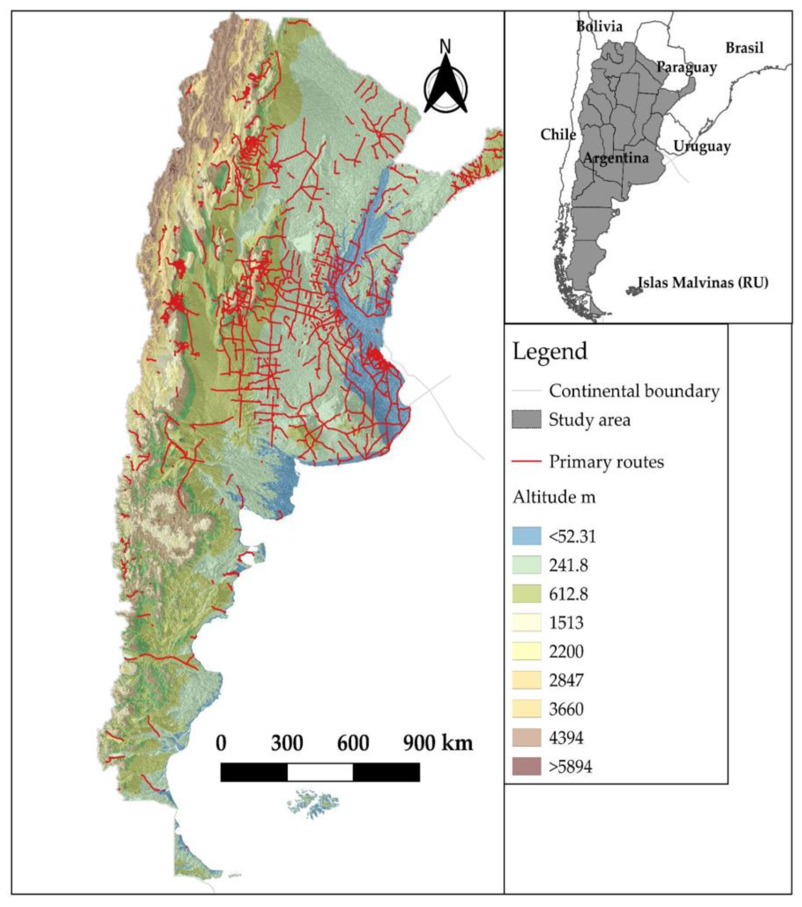
Figure 2.
The methodological flow.
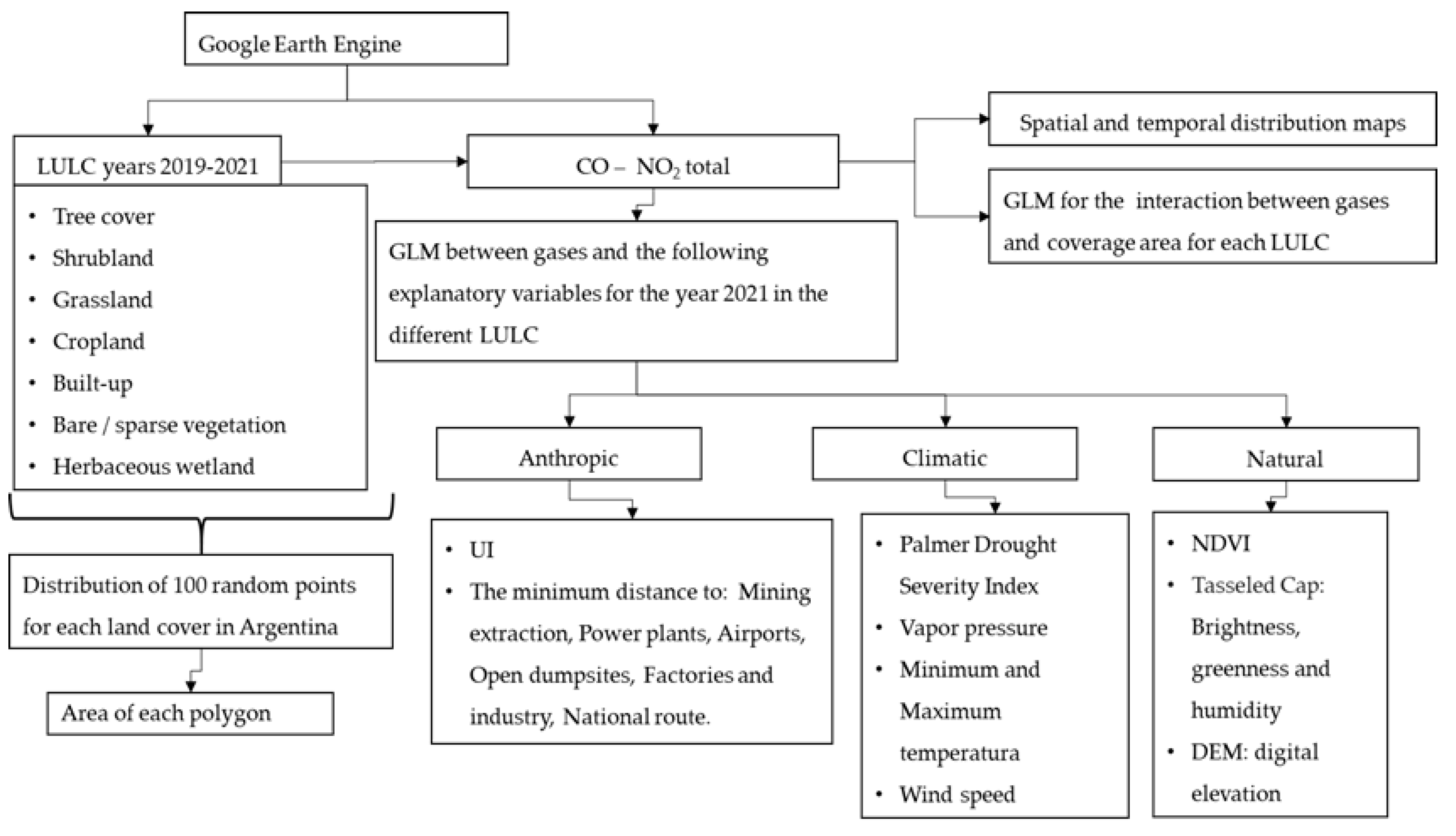
Figure 3.
Annual maps of CO distribution (mol/m-2) for Argentina.
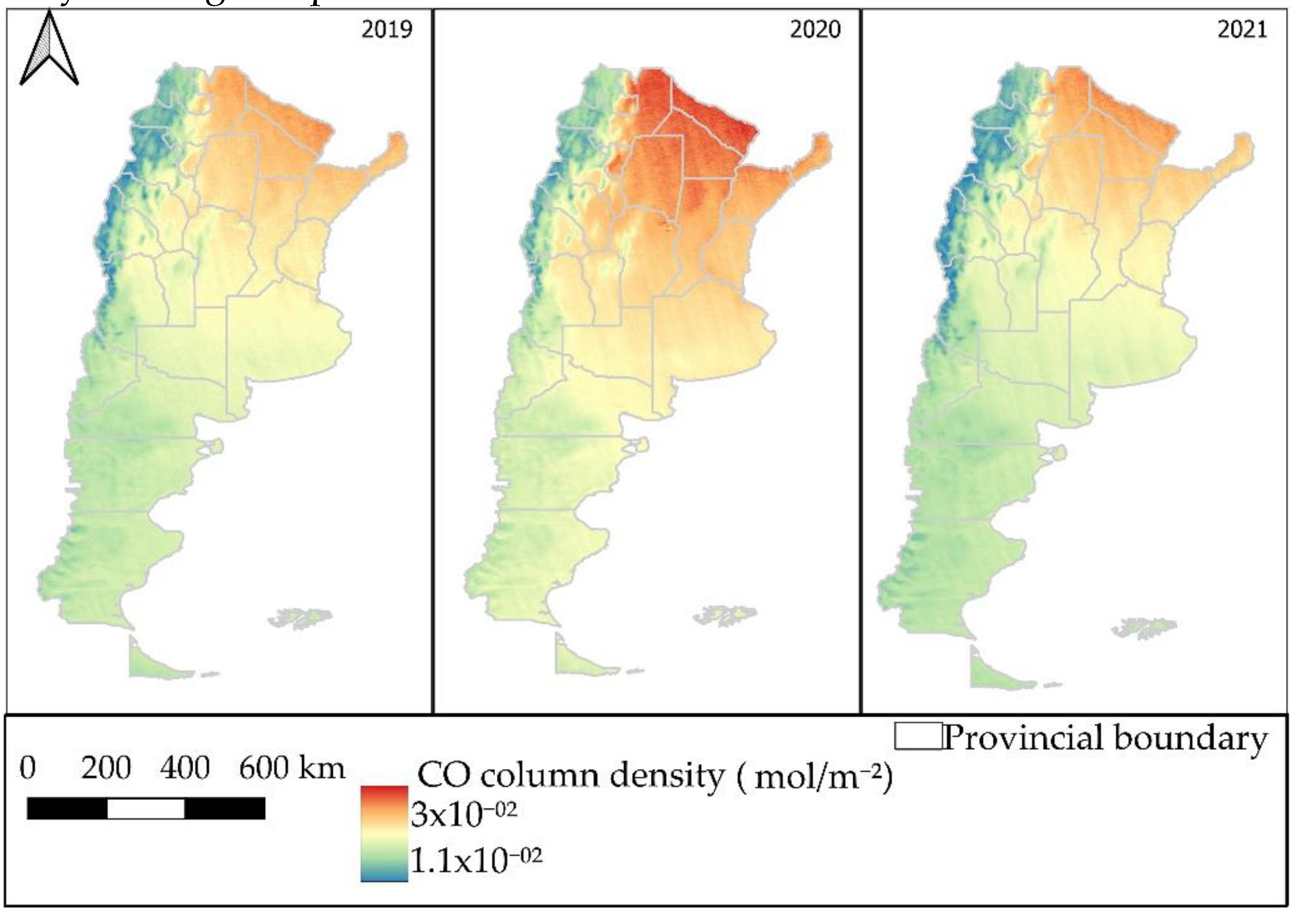
Figure 4.
Annual maps of NO2 distribution (mmol/m-2) for Argentina.
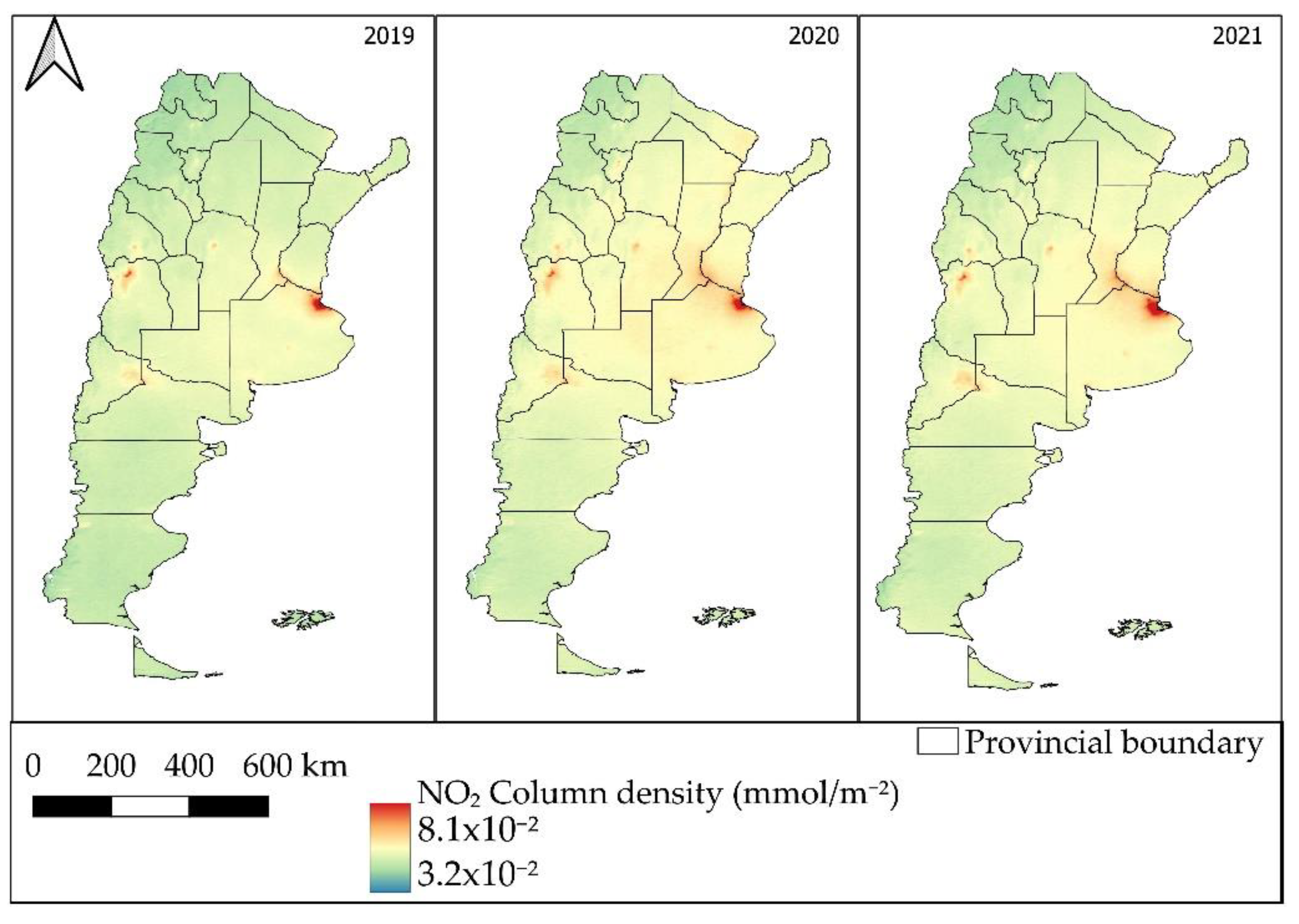
Figure 5.
Generalized linear model (global model) explaining the variation in NO2 concentration depending on the interaction between polygon area (ha) and LULC.
Figure 5.
Generalized linear model (global model) explaining the variation in NO2 concentration depending on the interaction between polygon area (ha) and LULC.
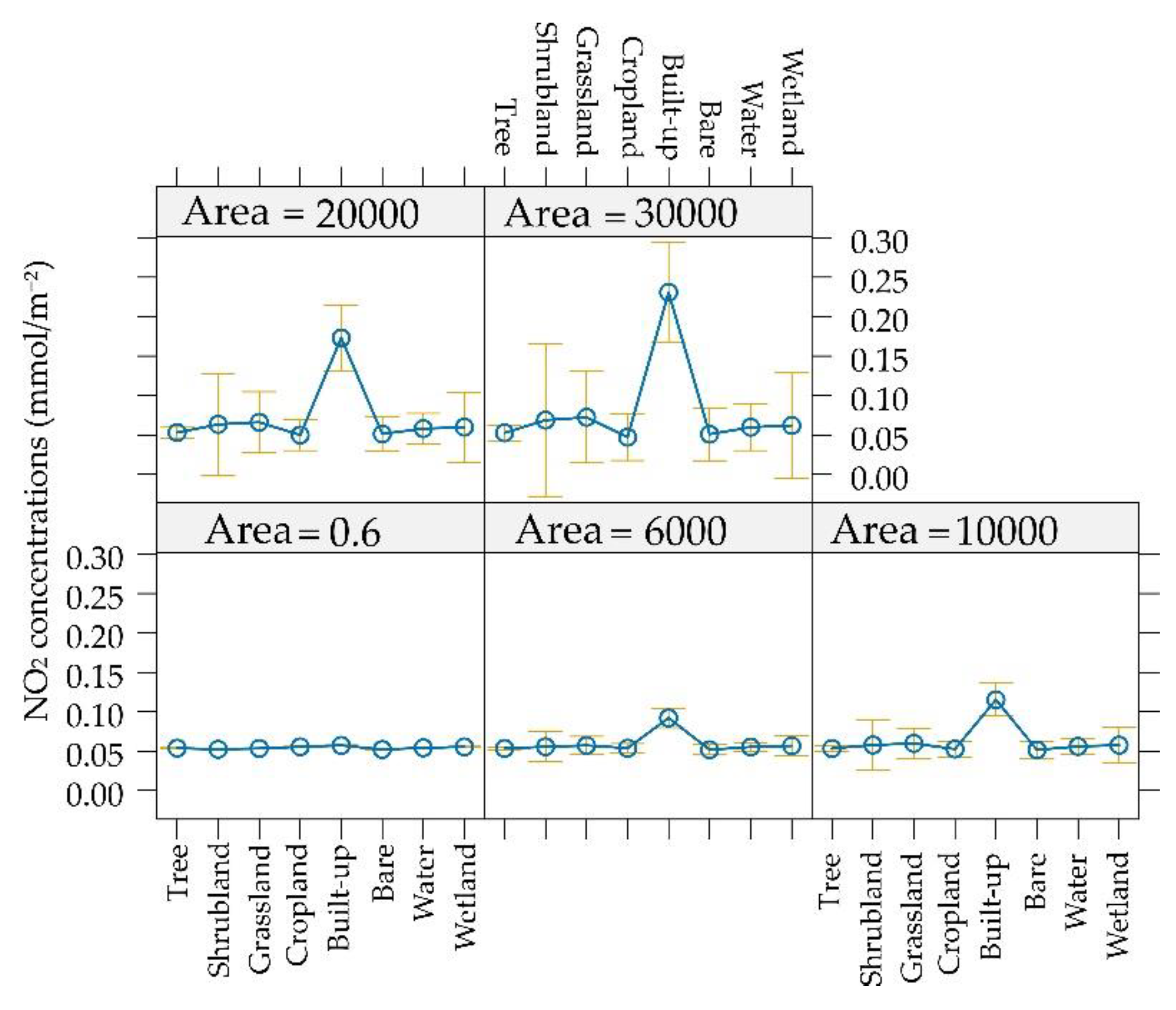

Table 1.
Generalized linear model (minimal adequate model) explaining the variation in the concentration of CO depending on anthropic, climatic, and natural indicators in the different LULC. The sign - indicates a negative relationship between the variables and the sign + indicates a positive relationship between the variables.
| CO | |||||
|---|---|---|---|---|---|
| Anthropic Predictors | National route | Mining extraction | Power plants | Airports | IU |
| Tree cover-Herbaceous wetland | - | - | |||
| Shrubland-Grassland | - | - | - | ||
| Cropland-Built-up | - | - | - | ||
| Bare/sparse vegetation | - | + | |||
| Climatic Predictors | Palmer Drought Index | Vapor pressure | Max environment temperature | Wind speed | |
| Tree cover-Herbaceous wetland | - | + | + | + | |
| Shrubland-Grassland | + | + | + | ||
| Cropland-Built-up | + | + | |||
| Bare/sparse vegetation | + | + | |||
| Natural Predictors | DEM | Humidity | NDVI | ||
| Tree cover-Herbaceous wetland | |||||
| Shrubland-Grassland | - | - | |||
| Cropland-Built-up | - | - | |||
| Bare/sparse vegetation | - |
Table 2.
Generalized linear model (minimal adequate model) explaining the variation in the concentration of NO2 depending on anthropic, climatic, and natural indicators in the different LULC. The sign - indicates a negative relationship between the variables and the sign + indicates a positive relationship between the variables.
| NO2 | |||||
|---|---|---|---|---|---|
| Anthropic Predictors | Service stations | Power plants | Airports | Open dumpsites | Factories-Industry |
| Tree cover-Herbaceous wetland | - | - | - | ||
| Shrubland-Grassland | - | - | |||
| Cropland-Built-up | - | - | |||
| Bare/sparse vegetation | - | ||||
| Climatic Predictors | Palmer Drought Index | Wind speed | |||
| Tree cover-Herbaceous wetland | - | - | |||
| Shrubland-Grassland | - | - | |||
| Cropland-Built-up | - | - | |||
| Bare/sparse vegetation | - | ||||
| Natural Predictors | DEM | NDVI | |||
| Tree cover-Herbaceous wetland | - | - | |||
| Shrubland-Grassland | - | ||||
| Cropland-Built-up | - | ||||
| Bare/sparse vegetation | - |
Disclaimer/Publisher’s Note: The statements, opinions and data contained in all publications are solely those of the individual author(s) and contributor(s) and not of MDPI and/or the editor(s). MDPI and/or the editor(s) disclaim responsibility for any injury to people or property resulting from any ideas, methods, instructions or products referred to in the content. |
© 2024 by the authors. Licensee MDPI, Basel, Switzerland. This article is an open access article distributed under the terms and conditions of the Creative Commons Attribution (CC BY) license (http://creativecommons.org/licenses/by/4.0/).
Copyright: This open access article is published under a Creative Commons CC BY 4.0 license, which permit the free download, distribution, and reuse, provided that the author and preprint are cited in any reuse.


