Submitted:
03 April 2024
Posted:
04 April 2024
You are already at the latest version
Abstract
This article describes an approach for optimising sensor-controlled systems through minimal intervention, utilising Fuzzy Linear Systems of Equations (FLSE). Staring with a generalised model of the system behaviour, incorporating an array of control units, environmental sensors, and an expert knowledge base. The described problems of detecting the level of intervention needed to change the system state to another is handled with the help of developed methods for solving the inverse problem for FLSE. By achieving minimal intervention, we ensure that system adjustments effective, economically optimal and non-intrusive. A MATLAB-based implementation is presented.
Keywords:
Sensor-Controlled Systems
; Fuzzy Linear Systems of Equations
; Inverse Problem
1. Introduction
This article focuses on a type of generalized sensor-controlled systems and introduces a method to alter their behavior while minimizing the level of intervention.
The described systems have the following components:
- An array of manageable control units
- A set of sensors providing information about the environment
- An expert knowledge module defining how the control units can change the environment
In that setup, assuming that we have a well defined expert knowledge, we can easily obtain information about the current status of the environment based on the sensor readings.
Let’s assume that now we want to change the environment status. The task, object to this article is to find the minimal possible change to the control units in order to achieve the new target state of the environment. I.e. if a system has a control units set to a state and the environment is in status , and if we want to achieve environment state , in this article we will answer the question of how to change the control units state to , so that the difference between and will be minimal.
Remark 1.
Assuming that we use sensors to measure the environment status, we will use the terms sensor readings, environment status, and system behavior as interchangeable.
In the following sections we will use a fuzzy rule-based expert knowledge base to represent our knowledge about how the control units influence on the environment. We will solve the inverse problem in fuzzy relational calculus [1,2,3] to find all possible changes to the control units, leading to the desired environment state, and will select the one closest to the current control units state.
We will use a fuzzy linear systems of equation (FLSE) of type (see Chapter Section 3).
The fairly direct approach for this task is to use a fuzzy inference system [4,5,6,7,8,9] and [10] to define our knowledge base as a set of fuzzy if-then rules. Then we can represent those rules as a FLSE (Section 3). Such representation is discussed and implemented in [11]. Another, more candid approach it to directly define the relation between the control units values and the expected sensor reading with FLSE, where the fuzzy matrix (FM) A will represent our knowledge base, the fuzzy matrix X will represent level of activation for the control units, and the matrix B will represent the achieved environment status.
2. Sensor Controlled System Examples
For the sake of completeness, let’s look at a few examples of sensor-controlled systems based on the architecture represented by Figure 1. Many other examples can fall in that architecture.
2.1. Smart Home System
These systems may use an array of sensors to monitor environmental conditions like temperature, humidity, and light, along with manageable control units like thermostats, blinds, and lights. The expert knowledge module might consist of rules about the homeowner’s preferences to adjust settings for optimal comfort and energy efficiency.
2.2. Automated Industrial Manufacturing Line
In these systems, sensors may collect data on machine performance (e.g. time to produce a single unit), product quality (e.g. analyzing final product photos), and environmental conditions. Control units may include conveyor belts, robotic arms or CNC machines speed control, humidity control, etc. The expert knowledge module would use rules to optimize production processes, reduce waste, and maintain quality standards. In separate moments we may need faster production sacrificing on the quality, or better quality sacrificing on the production speed performance.
2.3. Precision Agriculture Systems
These utilize sensors to monitor soil moisture, nutrient levels, and crop health. Manageable control units might involve irrigation systems, fertilizer spreaders, and spraying drones. The system’s expert knowledge may include rules to optimize watering schedules, fertilizer application, and pest control, based on the current environment status, ensuring maximal crop yield.
2.4. Health Monitoring Systems
Having sensors tracking health status metrics like heart rate, blood oxygen levels, and blood pressure levels. The control units could include notification systems or interfaces that communicate with other devices like medication dispensers. The expert knowledge implements rules to send alerts or adjust medication takings based on recommendations for the user.
3. Fuzzy Linear Systems of Equation (FLSE)
To represent the sensor-controlled system we will use a FLSE having one of the forms:
or
Where the operations ∧ and ∨, are respectively taking minimum and taking maximum, and the operations and , are according to the following Table 1 for :
A generalized matrix representation of equations (2) and (1) is:
where the fuzzy matrix (FM) A represents our knowledge of the system, the FM X represent the control units settings, and the FM B represents the system behavior. Operation can be any fuzzy multiplication (or fuzzy relational compositions) between A and X. For instance can be (or ), (or ), (or ), etc.
FLSE based on different fuzzy relational compositions are studied in details over the years - see [1,3,12,13,14,15,16,17,18,19]. In what follows we will focus on the composition, which is the most popular one. The presented method will be applicable by analogy for every other fuzzy relation composition in Table 1.
Therefore, we will use FLSE in the form:
or
4. Direct and inverse problems
The set forth in this chapter is according to [15]. The finite FMs and are called conformablein this order, if the number of columns in A is equal to the number of rows in B.
Definition 1.
Let and be finite conformable FMs. Obtaining the matrix , written is called productof A and B, if for each , it holds:
Definition 2.
When the finite conformable FMs A and X are given, computing the product is calleddirect problem resolutionfor the composition of the matrices A and X.
Direct problem is solvable in polynomial time. Software for direct problem resolution is given in [20,21,22]. It provides all the operations and algorithms described in Table 1 in MATLAB environment.
Definition 3.
When the finite conformable FMs A and B are given, computing the unknown matrix X is calledinverse problem resolutionfor the FLSE.
Inverse problem is solvable in exponential time. Software for inverse problem resolution is also given in [20,21,22]. It provides solvers for all the compositions in Table 1 in MATLAB environment.
4.1. Solutions of the inverse problem for (5)
For the fuzzy vectors and the inequality holds iff for each .
A vector with , , is called solution of the system (5) if holds. The set of all solutions of the system is called complete solution set and it is denoted by . If then the system is called solvable (or consistent), otherwise it is called unsolvable (or inconsistent).
A solution is called upper solution if for any the inequality implies . A solution is called lower solution if for any the inequality implies . If the upper solution is unique, it is called greatest (or maximum) solution. The n-tuple with is called interval solution if any with for each implies . Any interval solution whose components (interval bounds) are determined by the greatest solution from the right and by a lower solution from the left, is called maximal interval solution of (5).
It is well known [1,15], that any solvable fuzzy linear system of equations has unique greatest solution and one or many lower solutions. All the solutions in between the greatest solution and any of the lower solutions are also a solutions of (5). In order to find all solutions of the solvable system (5), it is necessary to find both its greatest solution and all of its lower solutions. Finding the greatest solution is relatively simple task often used as a criteria for establishing solvability of the system [14]. Finding all lower solutions is much more complex (from computational point of view) task, and is reasonable only when the lowest solution exists.
5. Adjusting the Sensor Control System Behavior with Minimal Intervention
Let’s have a sensor controlled system called S, described by fuzzy linear system of equation (5): . We can obtain its current behavior (or environment status) through the control units status and the knowledge base. When we represent our knowledge base with the fuzzy matrix A, and our control units settings with the fuzzy vector X - we can either solve the direct problem in FLSE to obtain the current system status or simply check it’s sensor readings. In case we want to adjust (or change) its behavior we will need to solve the inverse problem. I.e. we can describe the new, target behavior through the fuzzy vector B. Then we can solve the inverse problem in FLSE in order to achieve one or many possible ways to achieve this new status, then we need to adjust the system, so that the new control units settings cover one of the possible solutions of the inverse problem. Finally, if we want to achieve minimal adjustment to the system and still achieve the new target status, we need to choose such a solution of the inverse problem, so that the difference between the current control status and the target status is minimal. This process is described in the following algorithm:
| Algorithm 1:Change system status with minimal intervention |
|
Remark 2.
Step 2 is given for completeness. In most cases more accurate information can be obtained directly from the sensor readings. However, it can be a valid step if we experience sensor malfunction, or if we want to validate either of out knowledge base or the accuracy of the sensors.
Algorithm 1, while straightforward, includes several steps that require further elaboration.
5.1. Step 1: Detect Current System Status
This step is described by Definition 1 and Definition 2. To approach this task, we will simply need to calculate the product of the matrices A and . In the following example, we will utilize the software from [22] for this calculations.
5.2. Step 3: Solve the Inverse Problem
This step is the most complex for the Algorithm 1. It is subject of great scientific interest. The main results are published in [1,2,3]. They demonstrate long and difficult period of investigations for discovering analytical methods and procedures to determine the complete solution set, as well as to develop software for computing solutions. The first and most essential are Sanchez results [23] for the greatest solution of fuzzy relational equations with max-min and min-max composition. Sanchez gave formulas that permit to determine the potential greatest solution in any of these cases, often used as solvability criteria. Universal algorithm and software for solving max-min and min-max fuzzy relational equations is proposed in [3], and [13]. The relationship with the covering problem is subject of [12]. Systems of fuzzy relation equations and fuzzy relation inequalities, based on different fuzzy relational compositions are studied in details in [1,3,12,13,14,15,16,17,18,19].
The most advance software implementation for solving the inverse problem is developed by the author [15,21,22]. It includes algorithm implementation for eight popular fuzzy composition (including the composition). In the following examples we will use the software from [22] to find the complete solution set for the inverse problem for the system . This software features a great performance in finding the complete solution set, even for relatively large systems. For more information about the computational and memory complexity, as well as experimental results and comparison with the other available software, see [22].
5.3. Step 6: Find the Closest to the Current State, Solution
For the system 5, every interval described by the greatest solution from the right the any of its lower solutions from the left is called interval solution. Any value inside the interval solution is still a solution of the system [1,15]. Therefore the system 5, has as many interval solutions as many lower solutions. In order to find the solution (as a fuzzy vector), which is closest to some other fuzzy vector (in our case, the initial control units settings) we can use the following straightforward algorithm:
| Algorithm 2:Find the closest solution |
|
6. Example and MATLAB Execution
Example 1.
Let’s have a FLSE. It’s knowledge base will be represented by the FM A:
This system has 5 sensors modeling the environment status a 3 rules describing how the environment parameters (B) will change depending on the values (normalized as a fuzzy number) of the sensors (X). Each sensor reading have it’s own level of importance in each rule.
In this example we will use the following sensor readings as a starting point for the system:
Let’s implement Algorithm 1. We will use the software from [22] and will execute the algorithm steps in MATLAB.
6.1. Algorithm 1, Step 1 - Initialize FMs
>> A = fuzzyMatrix([.5 .6 .4 .1 .4; .1 .4 .1 .2 0; .9 .5 .2 .2 .9])
A =
3x5 fuzzyMatrix:
double data:
0.5000 0.6000 0.4000 0.1000 0.4000
0.1000 0.4000 0.1000 0.2000 0
0.9000 0.5000 0.2000 0.2000 0.9000
>> X = fuzzyMatrix([.9; .5; .5; .3; .9])
X =
5x1 fuzzyMatrix:
double data:
0.9000
0.5000
0.5000
0.3000
0.9000
6.2. Algorithm 1, Step 2 - Predict the Environment Status
>> B = maxmin(A,X)
B =
3x1 fuzzyMatrix:
double data:
0.5000
0.4000
0.9000
The system has 3 environment parameters. By executing this step, we can see in what degree every ot this parameters is currently observed.
6.3. Algorithm 1, Step 3 - Define New Target System Status
Now let’s assume that we want to achieve another environment status by lowering the level of degree with witch the third parameter is present (. Let’s try with two options - , and for which and will remain the same, but we will try it lower first to , and then to
>> B_new_1 = fuzzyMatrix([.5; .4; .4])
B_new_1 =
3x1 fuzzyMatrix:
double data:
0.5000
0.4000
0.4000
>> B_new_2 = fuzzyMatrix([.5; .4; .5])
B_new_2 =
3x1 fuzzyMatrix:
double data:
0.5000
0.4000
0.5000
6.4. Algorithm 1, Step 4 - Solve the Inverse Problem`
Now we create two FLSE (one for and one for , and solve them. The accepted parameters for the solve_inverse function are:
- The composition of the FLSE - In our case this will be
- The matrix A
- The matrix B
- The matrix X - this is what we will try to find, so we can pass an empty array here
- A Boolean parameter to flag if we need to find the complete solution set, or just the greatest solution
We solve both of the systems:
>> S1 = fuzzySystem(’maxmin’, A, B_new_1, [], true)
S1 =
fuzzySystem with properties:
composition: ’maxmin’
a: [3x5 fuzzyMatrix]
b: [3x1 fuzzyMatrix]
x: [5x1 fuzzyMatrix]
full: 1
inequalities: 0
>> S1.solve_inverse
ans =
fuzzySystem with properties:
composition: ’maxmin’
a: [3x5 fuzzyMatrix]
b: [3x1 fuzzyMatrix]
x: [1x1 struct]
full: 1
inequalities: 0
>> S2 = fuzzySystem(’maxmin’, A, B_new_2, [], true)
S2 =
fuzzySystem with properties:
composition: ’maxmin’
a: [3x5 fuzzyMatrix]
b: [3x1 fuzzyMatrix]
x: [5x1 fuzzyMatrix]
full: 1
inequalities: 0
>> S2.solve_inverse
ans =
fuzzySystem with properties:
composition: ’maxmin’
a: [3x5 fuzzyMatrix]
b: [3x1 fuzzyMatrix]
x: [1x1 struct]
full: 1
inequalities: 0
6.5. Algorithm 1, Step 5 - Obtain Solutions
First lets obtain all the solutions for (i.e. )
>> S1.x
ans =
struct with fields:
rows: 3
cols: 5
help: [3x5 fuzzyMatrix]
gr: [5x1 double]
ind: [3x1 double]
exist: 0
contradict: 1
For we can see that S1.x.exists = 0, which means that the system is inconsistent (i.e. the target environment state cannot be obtained).
>> S2.x
ans =
struct with fields:
rows: 3
cols: 5
help: [2x5 fuzzyMatrix]
gr: [5x1 fuzzyMatrix]
ind: [3x1 double]
exist: 1
dominated: 3
help_rows: 2
low: [5x2 fuzzyMatrix]
For we can see that the system is consistent S2.x.exists = 1, and it has 1 greatest solution (S2.x.gr.size(2) = 1), and 2 lower solutions (S2.x.low.size(2) = 2).
6.6. Algorithm 1, Step 6 - Check for Consistency
For the system we already determined that it is inconsistent so the algorithm ends here. Further we will focus on the system .
6.7. Algorithm 1, Step 7 - Find the new control units settings
Let’s print the greatest and all the lower solutions of the system
>> S2.x.gr
ans =
5x1 fuzzyMatrix:
double data:
0.5000
0.5000
1.0000
1.0000
0.5000
>> S2.x.low
ans =
5x2 fuzzyMatrix:
double data:
0.5000 0
0.4000 0.5000
0 0
0 0
0 0
From the greatest solution and the two lower solutions we know that the system has two interval solution, which determines the complete solution set of :
Let’s find the closest to the initial X vector for both of the interval solutions:
>> closestVector_1 = min(max(X, S2.x.low(:,1)), S2.x.gr)
closestVector_1 =
0.5000
0.5000
0.5000
0.3000
0.5000
>> closestVector_2 = min(max(X, S2.x.low(:,2)), S2.x.gr)
closestVector_2 =
0.5000
0.5000
0.5000
0.3000
0.5000
We can see that it is the same vector for both interval solutions, so the new value for X should be:
That means that we will need to adjust just the first control unit, lowering it with and the last control unit setting lowering it again with . This it the minimal intervention that we can achieve in order to change the system behavior from B, to .
6.8. Algorithm Step 8
Depending on the real world implementation of the system, we now need to use our actuators connected to the first and the last control units, in order to adjust them to the target values.
7. Conclusion
In this article, a method for adjusting sensor-controlled systems with minimal intervention, is presented. It facilitates the methods for solving the direct and the inverse problems for fuzzy linear systems of equations (FLSE). While here we have a generalized approach, it should be relatively easy to use the same principles for mode specific systems. Using the presented here algorithms, we can ensure that the change we want to achieve is either not possible, or if possible - done with the minimal possible intervention. This is ensured from the algorithms backing the process of acquiring the complete solution set of the system (5), presented in [21].
For the software implementation of the provided here example, we use the software from [22], which is already proven to work efficiently, and able to find all possible lower solutions of the system - a complex, non-trivial task.
The most obvious next step in this research will be to introduce a method, as well as a way to evaluate, a new state of the system, which is closest to the target, in the cases, when the target in not possible (i.e. when the system (5) is not consistent.
Funding
This research received no external funding
Conflicts of Interest
The authors declare no conflicts of interest.
Abbreviations
The following abbreviations are used in this manuscript:
| FLSE | Fuzzy Linear Systems of Equations |
| FM | Fuzzy Matrix |
References
- B. De Baets, Analytical solution methods for fuzzy relational equations, in the series: Fundamentals of Fuzzy Sets, The Handbooks of Fuzzy Sets Series, D. Dubois and H. Prade (eds.), Vol. 1, Kluwer Academic Publishers, 2000, pp. 291-340.
- A. Di Nola, W. Pedrycz, S. Sessa and E. Sanchez, Fuzzy Relation Equations and Their Application to Knowledge Engineering, Kluwer Academic Press, Dordrecht, 1989.
- K. Peeva and Y. Kyosev, Fuzzy Relational Calculus-Theory, Applications and Software (with CD-ROM), In the series Advances in Fuzzy Systems - Applications and Theory, Vol. 22, World Scientific Publishing Company, 2004. Software downloadable from http://www.mathworks.com/matlabcentral/fileexchange/loadFile.do?objectId=6214.
- J.F. Baldwin, "Fuzzy logic and fuzzy reasoning," in Fuzzy Reasoning and Its Applications, E.H. Mamdani and B.R. Gaines (eds.), London: Academic Press, 1981.
- F. Esragh and E.H. Mamdani, "A general approach to linguistic approximation," in Fuzzy Reasoning and Its Applications, E.H. Mamdani and B.R. Gaines (eds.), London: Academic Press, 1981.
- J.-S. R. Jang and N. Gulley, The Fuzzy Logic Toolbox for Use with MATLAB, Massachusetts: MathWorks Inc., 1995.
- Mamdani EH, Assilian S (1975) An experiment in linguist synthesis with fuzzy logic controller. Int J Man-Mach Stud 7(1):1-13.
- Siler W, Buckley JJ (2004) Fuzzy expert systems and fuzzy reasoning. Wiley InterScience.
- Yager, R.R. , and Zadeh, L. A., "An Introduction to Fuzzy Logic Applications in Intelligent Systems", Kluwer Academic Publishers, 1991.
- L.A. Zadeh, "Making computers think like people," I.E.E.E. Spectrum, 8/1984, pp. 26-32.
- Z. Zahariev, Fuzzy reasoning through fuzzy linear systems of equations, “Proceedings of the Technical University - Sofia”, Volume 60, book 3, 58-66, 2010, ISSN 1311-0829.
- A. Markovskii, On the relation between equations with max-product composition and the covering problem, Fuzzy Sets Systems, 153, 2005, pp. 261–273.
- K. Peeva, Universal algorithm for solving fuzzy relational equations, Italian Journal of Pure and Applied Mathematics 19, 2006, pp. 9-20.
- K. Peeva, Resolution of Fuzzy Relational Equations – Method, Algorithm and Software with Applications, Information Sciences, 234 (Special Issue), 2013, 44-63, doi 10.1016/j.ins.2011.04.011, ISSN 0020-0255.
- K. Peeva, G. Zaharieva, and Z. Zahariev, Resolution of max-t-norm fuzzy linear system of equations in BL-algebras, AIP Conference Proceedings vol. 1789, 06 0005, 2016. [CrossRef]
- J. Ignjatović, M. Ćirić, Br. Šešelja, A. Tepavčević, Fuzzy relational inequalities and equations, fuzzy quasiorders, closures and openings of fuzzy sets, Fuzzy Sets and Systems Volume 260, 2015, 1-24. 2015.
- S. Yang, Some Results of the Fuzzy Relation Inequalities With Addition–Min Composition, IEEE Transactions on Fuzzy Systems, vol. 26, no. 1, 239-245, 2018. [CrossRef]
- K. Peeva, Universal algorithm for solving fuzzy relational equations. Journal De Mathematiques Pures Et Appliquees 19, 2006, 169–188. 2006; 19.
- X. Yang, Solutions and strong solutions of min-product fuzzy relation inequalities with application in supply chain, Fuzzy Sets and Systems, 384, 2020, 54–74.
- Z. Zahariev, Solving Max-min Relational Equations. Software and Applications, in International Conference “Applications of Mathematics in Engineering and Economics (AMEE’08)”, AIP Conference Proceedings, vol. 1067, G. Venkov, R. Kovatcheva, V. Pasheva (eds.), American Institute of Physics, 2008, 516-523.
- Z. Zahariev, Software package and API in MATLAB for working with fuzzy algebras, in International Conference “Applications of Mathematics in Engineering and Economics (AMEE’09)”, AIP Conference Proceedings, vol. 1184, G. Venkov, R. Kovatcheva, V. Pasheva (eds.), American Institute of Physics, ISBN 978-0-7354-0750-9, 2009, 434-350.
- Z. Zahariev, http://www.mathworks.com/matlabcentral/fileexchange/27046-fuzzy-calculus-core-fc2ore, 54 2024 (most recent update).
- E. Sanchez, Resolution of composite fuzzy relation equations, Information and Control, 30, 1976, pp. 38-48.
Figure 1.
System overview.
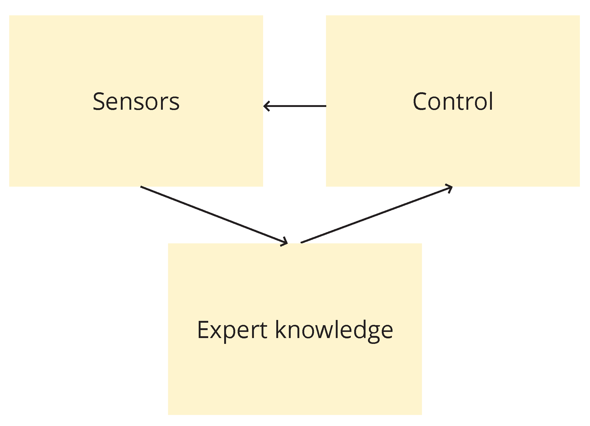

Table 1.
norms and norms
| t-norm | name | expression | s-norm | name | expression |
|---|---|---|---|---|---|
| minimum, Gödel norm | maximum, Gödel conorm | ||||
| Algebraic product |
Probabilistic sum | ||||
| ukasiewicz norm | Bounded sum |
Disclaimer/Publisher’s Note: The statements, opinions and data contained in all publications are solely those of the individual author(s) and contributor(s) and not of MDPI and/or the editor(s). MDPI and/or the editor(s) disclaim responsibility for any injury to people or property resulting from any ideas, methods, instructions or products referred to in the content. |
© 2024 by the authors. Licensee MDPI, Basel, Switzerland. This article is an open access article distributed under the terms and conditions of the Creative Commons Attribution (CC BY) license (http://creativecommons.org/licenses/by/4.0/).
Copyright: This open access article is published under a Creative Commons CC BY 4.0 license, which permit the free download, distribution, and reuse, provided that the author and preprint are cited in any reuse.


