
Submitted:
29 November 2024
Posted:
29 November 2024
You are already at the latest version
Abstract
The article considers the solution of control problems based on fuzzy logic. This approach allows to build decision support systems in various domains. The novelty of the approach is the algorithm for the generation of the fuzzy rules for a fuzzy controller based on the machine learning results interpretation to improve the quality of control actions in organizational and technical systems. Machine learning methods can find unknown patterns that require deep expert knowledge in some domain with a manual rules construction. We consider an example of the generation of a set of fuzzy rules based on the analysis of a decision tree model. It is possible to generate a set of fuzzy rules for constructing fuzzy inference system (FIS) based on the proposed algorithm. Membership functions and labels of linguistic terms are generated automatically for all input and output variables. The quality of the machine learning model and FIS were evaluated using the R2 metric. Experimental testing showed what the quality of FIS that is based on the generated fuzzy rules is worse by an average of 2 % compared to the original model based on the decision tree. The quality of FIS can be improved by tuning the membership functions, but this issue is beyond the scope of this article.
Keywords:
fuzzy logic
; fuzzy rules
; fuzzy inference system
; machine learning model interpretation
MSC: 90B50
1. Introduction
Control of the complex technical systems is a task based on the analysis of a large data volumes.
The quality of the results depends on the following factors:
- Control object complexity.
- Control task complexity.
- Volume of data for analysis.
- Time restrictions.
- Decisions urgency.
All these factors require the selection of a suitable class of mathematical models for control systems. First, we need to analyse the properties of a control object to determine the approach to solving a control problem.
General control theory defines requirements for the data and signals of the control object. It is also necessary to consider the data, features, and constraints of the external environment. In previous works, we show that the choice of a data analysis method and the quality of an analysis result are depends from a control problem context [1,2].
Fuzzy inference systems (FIS) are used to solve some classes of control problems. FIS allow to solve the control problem where data and expert knowledge may have some uncertainty. Then the properties of the control object and/or expert knowledge can be described in linguistic terms. Adapting a FIS to a specific task requires deep knowledge of the problem area. In some cases, an expert may not be available and machine learning methods can be used. However, in many problem areas, the results obtained in the machine learning process must be interpreted to evaluate the correctness.
Thus, we need to create an approach to generating a set of fuzzy rules for a fuzzy controller based on the machine learning results interpretation. This approach allows to reduce the complexity of analysis of a large data volumes and increase the interpretability of the analysis results.
2. Related Works
The management of complex technical systems requires an approach that ensures control stability, for example, based on the deterministic models. Intelligent components of a control system can identify behavior patterns of the object model based on analysis of the nonlinear and uncertain data with machine learning [3]. Component for predictive analytics plays a special role in control systems, because it allows to reduce the response time to emerging deviations. Quality of a control system is depends on the quality and volume of data, and form type and hyperparameters of a selected model as well.
Task of generating of a set of management rules is important and difficult because the quality of rules is influence to the quality of results of a control system, and an analytic needs to analyse the large volume of data to get rules with acceptable quality. The key feature of this task is the identification of features those influence on a quality of a control system result.
Various researchers use a different set of methods to generate a set of rules.
In paper [4] authors describe an approach to features extraction from a data.
In papers [5,6] described approaches for extraction a set of rules on data preparation stage based on a decision tree. Authors note that the approach based on a fuzzy rule base provides excellent opportunities for interpreting the results of data analysis. Authors also discusses a comparison of various methods for generating of a rule base based on a decision tree (ID3 algorithm), fuzzy decision tree, FUZZYDBD method. The authors propose an approach inspired by fuzzy decision tree approach based on ID3 algorithm that using information gain and Shannon’s entropy for feature selection criteria with fuzzification of the dataset.
In [7,8] authors consider the problem of the creation of control systems with fuzzy inference. Main problem is choosing the type of membership functions. The article also describes the algorithm for choosing the type of membership functions. The proposed approach is based on an algorithm to search for parameters of membership functions. Authors solve the problem of membership functions formation based on the statistical analysis of the features extracted from a training dataset. Researches focused on the original dataset as a basis for forming a high-quality classifying models.
Other researchers focused on the creation of fuzzy hierarchical systems [18,19,20,21]. In [9] consider the use of clusterisation based on fuzzy decision trees for multi-criteria decision making. Describing value intervals based on fuzzy sets allows to increase the flexibility of the system.
In the article [13] discussed the problem of constructing fuzzy decision trees, and the problem of choice of the type of membership functions.
In [10,11] authors describe approaches for creation of a control system based on a fuzzy rule bases generating with genetic evolutional algorithms. The main idea behind those approaches is finding an optimal solution to different problems based on analyzing large arrays of data.
Authors of [12,16,22] describe the usage of neuro-fuzzy networks to solve problems of nonlinearity of features of analysed objects in control tasks, for example, for energy storage systems.
The main problem of creating control systems based on fuzzy knowledge bases is the preparation of data and rule extraction. It is necessary to have a dataset with informative features to build a control system with acceptable quality [17]. Some methods require data labeling [14] or data preprocessing [7].
The options for improving the quality of a fuzzy control systems are:
- A high-quality result can be achieved by forming, normalizing, and optimizing a set of rules.
- It is necessary to select optimal membership functions and regulate their parameters to obtain high-quality results.
Rule mining approach can be based on rule classifier that was trained on existing labeled dataset [15].
Thus, existing approaches to the generation of rules for rule-based control systems cannot be used without deep knowledge of data analysis and statistics. Large amount of analytical work must be completed for high-quality tuning of hybrid models. Quality of the solution to the problem a rule generation and control problem itself is depend on expert opinion when need to choose the methods and their parameters and operating modes.
We define the main problem statement as the development of a method that allow to analyze the initial data in order to extract rules that have a high generalizing ability to identify patterns and operating modes of the control system [23]. Also, an approach to interpreting machine learning models can be used when developing such a method [24].
If non-deep machine learning methods cannot find patterns in the data, then it may be impossible to create a set of rules to achieve the required level of quality without deep expert knowledge.
3. Material and Methods
In Section 2 we presented an analysis of articles on the problem of generating fuzzy rules for FIS. That problem can be solved based on the interpretation and explanation of the results of machine learning models. Machine learning methods can find hidden patterns. Those patterns can be converted to a set of rules. The classical approach to the formation of a set of rules for a control system requires deep expert knowledge from an analytic.
In this paper, we propose an approach to generating fuzzy rules based on the analysis of a result of a machine learning model. The analysed model is created using a supervised learning algorithm based on decision trees.
3.1. Description of the Dataset
We used the dataset described in [25] to train the decision tree model. In [26], the authors used this dataset to create and evaluate a FIS-based control system. The dataset contains several tables. Each table contains measurements of the effect of the input parameters, aluminum oxide (Al2O3) and titanium dioxide (TiO2) dispersed in distilled water and ethylene glycol with 50:50 volumetric proportions on the density and viscosity parameters at different temperatures.
Thus, the input parameters from X are:
- Temperature (): 20-70 °C
- Al2O3 concentration (): 0, 0.05, 0.3 vol %.
- TiO2 concentration (): 0, 0.05, 0.3 vol %.
Output parameters from Y are:
- Density ().
- Viscosity ().
The Appendices Appendix A and Appendix B present the used datasets. Each dataset is divided into training and test sets.
3.2. Schema of the Proposed Approach
The Figure 1 shows the schema of the proposed approach to extracting fuzzy rules for constructing FIS based on the interpretation of decision tree results.
As you can see from the Figure 1, the input data is the training part of a dataset.
The CART algorithm [27] was chosen as the algorithm for training the model for creating a binary decision tree. The CART algorithm has the following advantages:
- There is no need to calculate and select various parameters to execute the algorithm.
- There is no need to pre-select the variables that will participate in the analysis to apply the algorithm. The variables are selected during model training based on the Gini index value.
- The algorithm handles outliers well. Separate tree branches are formed for data with outliers.
- High model training speed.
The major disadvantage of the CART algorithm is the low quality of the model for data with many dependencies between features. The solution to this problem is not covered in this article and will be solved in the future. The quality of the decision tree-based model is evaluated using the metric [27].
The decision tree model is formed after the CART algorithm execution. The decision tree model is the input data for the proposed approach to the generation of fuzzy rules. A set of fuzzy rules is generated as a result.
The resulting fuzzy rules are used to build FIS. The fuzzy rule can be represented as:
where is the antecedent (condition) of the fuzzy rule; is the consequent (result) of the fuzzy rule; are the i-th and j-th atoms of the antecedent and consequent, respectively; is an operator for connecting the atoms of the rule. and operators can be interpreted as functions of or depending on the fuzzy inference algorithm.
The operation of FIS is based on the principles of Zadeh’s fuzzy logic [28]. The operation of FIS can be described as a sequence of the following steps:
- Fuzzification of input values. The value of the input variable is assigned a set of linguistic terms of some fuzzy variable during fuzzification. Each fuzzy variable can be described as:where N is the variable name: temperature, concentration; T is a set of linguistic terms: high temperature, medium temperature, low temperature, high concentration, medium concentration, low concentration; U is an range of values; F is a function for calculating the degree of membership of the input variable value to a certain linguistic term. The set of linguistic terms describes a subset of values of the fuzzy variable U. In this case, the value of the input variable is related to all linguistic terms with different membership degrees .
-
Aggregation. Truth degree of the rule antecedent is calculated at the aggregation stage:Each atom of the antecedent of a fuzzy rule corresponds to a linguistic term of some fuzzy variable . Rule atoms are replaced by the values of the membership degree of the input variable to some linguistic term during aggregation,. Then the function ( or ) is applied. The implementation of the function is determined by the algorithm of fuzzy logical inference: Mamdani, Sugeno, Tsukamoto, etc.
- Activation. Truth degree of the consequent of the output variable is calculated at the activation stage,. In our case, the consequent always consists of one atom and has a weight coefficient equal to 1. Thus:
- Accumulation. The membership function is formed for all output variables at the accumulation stage. The membership function is formed based on the max-union of the membership degrees of all linguistic terms of i-th fuzzy variable :
- Defuzzification. Numerical value for the fuzzy output variable is obtained based on the membership function at the defuzzification stage. In our case, the Centre of Gravity method is used:
The quality of FIS is evaluated on the test part of a dataser using the metric and compared with the value for the decision tree model.
The primary aim of this study is to confirm the Hypothesis 1.
Hypothesis 1.
It is possible to generate a set of fuzzy rules for constructing FIS based on the proposed algorithm. The quality of FIS must not be much worse in quality compared to the original decision tree model. Membership functions and labels of linguistic terms are generated automatically for all input and output variables. It is only necessary to specify the required number of terms: 3 or 5.
3.3. Description of the Approach to Generating Fuzzy Rules
In this section, we will consider the operation of the proposed approach to generating fuzzy rules using the example of constructing a FIS to determine the value of the output variable based on the values of the input variables , , and . The data set is presented in the Table A1.
Decision tree was created based on the training sample using the CART algorithm. Indicator was calculated based on the test data set for the decision tree . The resulting decision tree model was saved in a file for further use.
Step 1. Get a set of raw rules from the decision tree
Set of raw rules is extracted from the previously created decision tree at the first step of the proposed approach.
Formally, a rule extracted from a decision tree can be represented as:
where is the rule antecedent; is the rule antecedent atom that describes the constraint of some input variable x with type and value ; is the rule consequent that determines the value of the output variable .
Extraction of a set of raw rules is performed based on the algorithm described in the work [30].
A raw rule is a rule that is extracted from a decision tree and contains an excessive number of conditions that may overlap, for example:
A set of raw rules is presented in the Appendix C.
In the rule presented above, several conditions are imposed on the value of the input variables. These conditions must be simplified by performing normalization of the rules.
Step 2. Normalization of raw rules
Set of normalized rules is formed from the set of raw rules at the second step of the proposed approach. It is necessary to remove intersecting conditions from the raw rule for all input variables to obtain a normalized rule . The normalization function can be represented as the Algorithm 1.
| Algorithm 1 Rules normalization algorithm |
|
As you can see from the description of the Algorithm 1 algorithm, set of atoms is searched in the antecedent of each raw rule . The set contains the atoms of the rule antecedent that are associated with the input variable . Then, the search for atoms with the ≤ type is performed and the atom with the maximum value of the parameter is selected. Search for the atom with the minimum value of the parameter is performed among the atoms with the > type. The antecedent of the normalized rule is formed based on the found atoms and . The consequent of the normalized rule is the consequent of the raw rule .
An example of a normalized rule is shown below:
The set of normalized rules is presented in the Appendix D.
The Algorithm 1 forms a set of normalized rules . Normalized rules may have equivalent antecedents and different consequents. We call such rules as similar. Similar rules must be reduced to a single rule.
Step 3. Removing Similar Rules
The third step of the proposed method involves removing similar rules. Similar rules are rules with equivalent antecedents. Algorithm 2 formally represents the function of removing similar rules.
| Algorithm 2 Algorithm for removing similar rules |
|
As you can see from the description of the Algorithm 2 algorithm, a list of similar rules is formed at the first step. The get_similar_rules function is used to determine similar rules. Rules with equivalent antecedents are similar. Then a list containing rules for which there are no similar rules in the original set is formed. The reduced set is formed on the basis of the set of similar rules by grouping the rules by equivalent antecedents. The consequents for the rules of the reduced set are calculated as the arithmetic mean of the consequents of the rules grouped by equivalent antecedents. The group_rules function is used to group the rules. The result of the algorithm is the union of the sets and ()
Let’s consider an example of the execution of the Algorithm 2. Before execution of the algorithm , after execution of the algorithm – . Example of a similar rules removing:
The set of normalized rules after removing similar rules is presented in the Appendix E.
Next, it is necessary to move from the intervals of values of the atoms of the rules antecedents to specific values.
Step 4. Rules simplification
It is necessary to move from intervals in the atoms of the rule antecedents to specific values of variables after removing similar rules. Rules simplification is allow applying fuzzification to construct fuzzy rules.
Rules simplification can be represented as an Algorithm 3.
| Algorithm 3 Rules simplification algorithm |
|
As you can see from the description of the 3 algorithm, the left part of the interval n and the right part of the interval m are searched for each input variable in the antecedent atom of the rule . If the antecedent of the rule contains both parts of the interval, then the average value of the parameter of the atoms n and m is specified as the value of the simplified atom . If the antecedent of the rule contains only the left part of the interval n, then the value of the new atom is set as the minimum value of the variable in the data set . If the antecedent of the rule contains only the right part of the interval m, then the value of the new atom is set as the maximum value of the variable in the data set . New antecedent of the rule is formed based on the the process of atoms simplification, the consequent remains unchanged.
Figure 2 is schematically presented the Algorithm 3.
Let’s look at an example of simplified rules:
The set of simplified rules is presented in the Appendix F.
It is necessary to form fuzzy sets for the input variables and form a set of fuzzy rules based on atom fuzzification after simplifying the rules.
Step 5. Rule fuzzification
It is necessary to form fuzzy sets for the input and output variables to fuzzify the set of rules :
The automatic method [32] of generation of fuzzy sets for crisp variables is used as an implementation of the function. Thus, a corresponding fuzzy variable (, ) is formed with the specified number of linguistic terms n for each variable (, ).
The Figure 3, Figure 4, Figure 5 and Figure 6 present the automatically generated fuzzy sets for the variables , , and , respectively.
Next, the Algorithm 4 generates a set of fuzzy rules based on a set of simplified rules .
| Algorithm 4 Fuzzy rules generation algorithm |
|
As you can see from the description of the 4 algorithm, fuzzification function is executed for each atom of the antecedent of the crisp rule . m set is formed after fuzzification. Each element of the set contains the membership degree of the crisp variable to the linguistic term of the fuzzy variable . An atom of the fuzzy rule is formed using the function max based on the set m. Thus, the atom of the fuzzy rule contains a reference to the fuzzy variable , as well as the degree of membership in the linguistic term . Atom of a consequent is formed similarly to the atoms of an antecedent.
Let’s consider an example of fuzzy rules:
Rules with similar antecedents and different consequents may be formed after 4 algorithm executing. Algorithm 2 is used to delete similar fuzzy rules. This algorithm was adapted to work with fuzzy rules. A special function group_fuzzy_rules (Algortihm 5) was developed to group fuzzy rules.
| Algorithm 5 Group fuzzy rules algorithm |
|
As you can see from the description of the 5 algorithm, the group_fuzzy_rules function remains only one of the similar rules in which the antecedent atoms have the minimum total value of membership degrees .
The set of simplified rules is presented in the Appendix G. The number of rules in the set before fuzzification , and after fuzzification .
It becomes possible to perform fuzzy inference to get the value of the output variables Y based on the input variables X after obtaining the set of fuzzy rules.
Step 6. Fuzzy Inference
Fuzzy inference allows to get the value of crisp output variables Y based on crisp input variables X. Fuzzy rules are used in the inference process to describe an expert knowledge as the functional dependence .
For example, for input variables , , and :
-
Fuzzification:
- , , ;
- , , ;
- , , .
-
Aggregation and activation:
-
For rule:;
-
For rule:;
-
For rule:, etc.
-
- Accumulation. Figure 7 represents the accumulation result.
- Defuzzification. .
3.4. Rules Clustering
Rule clustering allows to grouping the rules based on the parameters of the rule antecedent atoms. The groups of rules allow an expert to evaluate the rules and set the hyperparameters for the proposed fuzzy rule generation method. The proposed rule clustering algorithm can be used for crisp and fuzzy rules.
For example, such groups in the A1 data are rows 1–9, 10–15, etc. It is necessary to specify a set of input variables to combine rules into groups. Atoms of a rule antecedent are selected based on selected input variables. For example, clustering can be performed in the A1 data set based on atoms with the and variables. Atoms with the variable can be ignored, because the variable value is repeated in each group of data rows. The set of variables is a hyperparameter of the rule clustering algorithm. Only atoms that are associated with the variables or (the parameter of the atom x) are used in this example. The variable was excluded.
It is necessary to vectorize the rules to perform clustering. The algorithm for generating a unique list of atoms is presented in 6.
| Algorithm 6 Algorithm for generating a unique list of atoms |
|
As you can see from the description of the Algorithm 6, the result of the algorithm is a set of unique atoms extracted from the set of rules . Only atoms with a parameter whose value is not contained in the set of excluded variables are added to the set .
The following set of unique atoms is formed:
The set is used in the vectorization process as a binary mask. For example, for the rule the resulting vector is:
Process of automatic selection of clusters number is performed after vectorization. The minimum value of the clusters number is . The maximum value of the clusters number can be specified manually by the user or it can be calculated as . Automatic selection of clusters number is based on the value of the silhouette coefficient s [31]:
where a is the mean intra-cluster distance, b is the distance between a sample and the nearest cluster that the sample is not a part of. The best value is 1 and the worst value is -1. Values near 0 indicate overlapping clusters. Negative values indicate that a sample has been assigned to the wrong cluster, as a different cluster is more similar.
KMeans algorithm is used for clustering. n iterations of the clustering algorithm are sequentially performed for each . Silhouette coefficient is calculated (see Figure 8) for each iteration and the minimum value of the clusters number () with the maximum of the value is selected. Thus, the best value of was obtained at iteration when splitting into five clusters.
Result of the rules clustering is:
Full result of the rules clustering is presented in the Appendix H.
4. Experiments
We develop an application to test the hypothesis 1. The main parameters of the environment for the developed application include:
- Programming language: Python.
- Python interpreter version: 3.12.
-
Libraries:
- Machine learning library (decision tree and KMeans clustering): scikit-learn 1.5.2;
- Data manipulation libraries: numpy 2.1.0 and pandas 2.2.2;
- Fuzzy inference library: scikit-fuzzy 0.5.0;
- Plotting library: matplotlib 3.9.2;
- Additional dependency for the scikit-fuzzy library: networkx 3.4.2.
Decision tree models were created for the output variables and based on the training set of the A1 and A2 datasets. The following variables , , and were used as input variables in both experiments.
The following metric values were calculated for the resulting decision tree models based on the test set of the A1 and A2 datasets:
- ;
- .
Algorithm was extracted the following raw rules from the resulting decision trees:
- ;
- ;
The following rules were obtained after executing the algorithms for normalization and removal of similar rules:
- ;
- ;
Then, the proposed algorithm generated the following fuzzy rules:
- ;
- .
Automf algorithm from the scikit-fuzzy library [32] was used to generate all fuzzy sets. The number of linguistic terms is a hyperparameter of the proposed approach. We selected its value during the experiments.
The Table 1 contains the FIS results. The column Real contains real data, and the column Inferred is a result of fuzzy inference.
The following values of the metric were calculated for the FIS based on the test set of the Appendices A1 and A2 datasets:
- ;
- .
Let’s calculate the difference between the indicators for decision tree models and the FISs:
- ;
- .
The average difference in the metric is about 2 %. The hypothesis is proven.
5. Conclusions
We consider an approach to solving control problems based on fuzzy logic. This approach allow to develop decision support systems for various application areas. The article considering the example of generating a set of fuzzy rules based on the interpretation of a decision tree model. The limitations of the proposed approach is the ability to work with dataset on which the CART algorithm shows an acceptable result.
Future work plans include:
- Development of an approach to generating a set of fuzzy rules based on the interpretation of other machine learning algorithms.
- Development of a method for generating fuzzy sets, considering the specifics of the subject area to improve the FIS quality.
Author Contributions
Conceptualization, A.A.R.; data curation, A.A.F.; formal analysis, A.A.F.; methodology, N.G.Y.; visualization, A.A.R. All authors contributed equally. All authors have read and agreed to the published version of the manuscript.
Funding
This research was funded by the Ministry of Science and Higher This study was supported the Ministry of Science and Higher Education of Russia in framework of project No. 075-03-2023-143 ”The study of intelligent predictive analytics based on the integration of methods for constructing features of heterogeneous dynamic data for machine learning and methods of predictive multimodal data analysis”.
Institutional Review Board Statement
Not applicable.
Informed Consent Statement
Not applicable.
Data Availability Statement
Not applicable.
Conflicts of Interest
The authors declare no conflict of interest.
Appendix A. Density Dataset

Table A1.
The effect of input parameters , and on the output parameter .
| # | (°C) | (%) | (%) | |
|---|---|---|---|---|
| train dataset | ||||
| 1 | 20 | 0 | 0 | 1.0625 |
| 2 | 25 | 0 | 0 | 1.05979 |
| 3 | 35 | 0 | 0 | 1.05404 |
| 4 | 40 | 0 | 0 | 1.05103 |
| 5 | 45 | 0 | 0 | 1.04794 |
| 6 | 50 | 0 | 0 | 1.04477 |
| 7 | 60 | 0 | 0 | 1.03826 |
| 8 | 65 | 0 | 0 | 1.03484 |
| 9 | 70 | 0 | 0 | 1.03182 |
| 10 | 20 | 0.05 | 0 | 1.08755 |
| 11 | 45 | 0.05 | 0 | 1.07105 |
| 12 | 50 | 0.05 | 0 | 1.0676 |
| 13 | 55 | 0.05 | 0 | 1.06409 |
| 14 | 65 | 0.05 | 0 | 1.05691 |
| 15 | 70 | 0.05 | 0 | 1.05291 |
| 16 | 20 | 0.3 | 0 | 1.18861 |
| 17 | 25 | 0.3 | 0 | 1.18389 |
| 18 | 30 | 0.3 | 0 | 1.1792 |
| 19 | 40 | 0.3 | 0 | 1.17017 |
| 20 | 45 | 0.3 | 0 | 1.16572 |
| 21 | 50 | 0.3 | 0 | 1.16138 |
| 22 | 55 | 0.3 | 0 | 1.15668 |
| 23 | 60 | 0.3 | 0 | 1.15233 |
| 24 | 70 | 0.3 | 0 | 1.14414 |
| 25 | 20 | 0 | 0.05 | 1.09098 |
| 26 | 25 | 0 | 0.05 | 1.08775 |
| 27 | 30 | 0 | 0.05 | 1.08443 |
| 28 | 35 | 0 | 0.05 | 1.08108 |
| 29 | 40 | 0 | 0.05 | 1.07768 |
| 30 | 60 | 0 | 0.05 | 1.06362 |
| 31 | 65 | 0 | 0.05 | 1.05999 |
| 32 | 70 | 0 | 0.05 | 1.05601 |
| 33 | 25 | 0 | 0.3 | 1.2186 |
| 34 | 35 | 0 | 0.3 | 1.20776 |
| 35 | 45 | 0 | 0.3 | 1.19759 |
| 36 | 50 | 0 | 0.3 | 1.19268 |
| 37 | 55 | 0 | 0.3 | 1.18746 |
| 38 | 65 | 0 | 0.3 | 1.178 |
| test dataset | ||||
| 1 | 30 | 0 | 0 | 1.05696 |
| 2 | 55 | 0 | 0 | 1.04158 |
| 3 | 25 | 0.05 | 0 | 1.08438 |
| 4 | 30 | 0.05 | 0 | 1.08112 |
| 5 | 35 | 0.05 | 0 | 1.07781 |
| 6 | 40 | 0.05 | 0 | 1.07446 |
| 7 | 60 | 0.05 | 0 | 1.06053 |
| 8 | 35 | 0.3 | 0 | 1.17459 |
| 9 | 65 | 0.3 | 0 | 1.14812 |
| 10 | 45 | 0 | 0.05 | 1.07424 |
| 11 | 50 | 0 | 0.05 | 1.07075 |
| 12 | 55 | 0 | 0.05 | 1.06721 |
| 13 | 20 | 0 | 0.3 | 1.22417 |
| 14 | 30 | 0 | 0.3 | 1.2131 |
| 15 | 40 | 0 | 0.3 | 1.20265 |
| 16 | 60 | 0 | 0.3 | 1.18265 |
| 17 | 70 | 0 | 0.3 | 1.17261 |
Appendix B. Viscosity Dataset
Table A2.
Effect of input parameters , and on output parameter .
| # | (°C) | (%) | (%) | |
|---|---|---|---|---|
| train dataset | ||||
| 1 | 20 | 0 | 0 | 3.707 |
| 2 | 25 | 0 | 0 | 3.18 |
| 3 | 35 | 0 | 0 | 2.361 |
| 4 | 45 | 0 | 0 | 1.832 |
| 5 | 50 | 0 | 0 | 1.629 |
| 6 | 55 | 0 | 0 | 1.465 |
| 7 | 70 | 0 | 0 | 1.194 |
| 8 | 20 | 0.05 | 0 | 4.66 |
| 9 | 30 | 0.05 | 0 | 3.38 |
| 10 | 35 | 0.05 | 0 | 2.874 |
| 11 | 40 | 0.05 | 0 | 2.489 |
| 12 | 50 | 0.05 | 0 | 1.897 |
| 13 | 55 | 0.05 | 0 | 1.709 |
| 14 | 60 | 0.05 | 0 | 1.47 |
| 15 | 20 | 0,3 | 0 | 6.67 |
| 16 | 25 | 0,3 | 0 | 5.594 |
| 17 | 30 | 0,3 | 0 | 4.731 |
| 18 | 35 | 0,3 | 0 | 4.118 |
| 19 | 40 | 0,3 | 0 | 3.565 |
| 20 | 55 | 0,3 | 0 | 2.426 |
| 21 | 60 | 0,3 | 0 | 2.16 |
| 22 | 70 | 0,3 | 0 | 1.728 |
| 23 | 20 | 0 | 0.05 | 4.885 |
| 24 | 25 | 0 | 0.05 | 4.236 |
| 25 | 35 | 0 | 0.05 | 3.121 |
| 26 | 40 | 0 | 0.05 | 2.655 |
| 27 | 45 | 0 | 0.05 | 2.402 |
| 28 | 50 | 0 | 0.05 | 2.109 |
| 29 | 60 | 0 | 0.05 | 1.662 |
| 30 | 70 | 0 | 0.05 | 1.289 |
| 31 | 20 | 0 | 0.3 | 7.132 |
| 32 | 25 | 0 | 0.3 | 5.865 |
| 33 | 30 | 0 | 0.3 | 4.944 |
| 34 | 35 | 0 | 0.3 | 4.354 |
| 35 | 45 | 0 | 0.3 | 3.561 |
| 36 | 55 | 0 | 0.3 | 2.838 |
| 37 | 60 | 0 | 0.3 | 2.538 |
| 38 | 70 | 0 | 0.3 | 1.9097 |
| test dataset | ||||
| 1 | 30 | 0 | 0 | 2.716 |
| 2 | 40 | 0 | 0 | 2.073 |
| 3 | 60 | 0 | 0 | 1.329 |
| 4 | 65 | 0 | 0 | 1.211 |
| 5 | 25 | 0.05 | 0 | 4.12 |
| 6 | 45 | 0.05 | 0 | 2.217 |
| 7 | 65 | 0.05 | 0 | 1.315 |
| 8 | 70 | 0.05 | 0 | 1.105 |
| 9 | 45 | 0.3 | 0 | 3.111 |
| 10 | 50 | 0.3 | 0 | 2.735 |
| 11 | 65 | 0.3 | 0 | 1.936 |
| 12 | 30 | 0 | 0.05 | 3.587 |
| 13 | 55 | 0 | 0.05 | 1.953 |
| 14 | 65 | 0 | 0.05 | 1.443 |
| 15 | 40 | 0 | 0.3 | 3.99 |
| 16 | 50 | 0 | 0.3 | 3.189 |
| 17 | 65 | 0 | 0.3 | 2.287 |
Appendix C. Raw Rules Set rraw
Appendix D. Set of normalized rules rnorm
Appendix E. Set of normalized rules rnorm after removing similar rules
Appendix F. A set of simplified rules rsimp
Appendix G. The set of fuzzy rules rfuzz
Appendix H. Result of grouped rules
References
- Romanov, Anton A., Aleksey A. Filippov, and Nadezhda G. Yarushkina. "Adaptive Fuzzy Predictive Approach in Control." Mathematics 11.4 (2023): 875. [CrossRef]
- Romanov, Anton, and Aleksey Filippov. "Context modeling in predictive analytics." 2021 International Conference on Information Technology and Nanotechnology (ITNT). IEEE, 2021.
- Xu, J.; Wang, Q.; Lin, Q. Parallel robot with fuzzy neural network sliding mode control. Adv. Mech. Eng. 2018, 10, 1687814018801261. [CrossRef]
- Kerr-Wilson, Jeremy, and Witold Pedrycz. "Generating a hierarchical fuzzy rule-based model." Fuzzy Sets and Systems 381 (2020): 124-139. [CrossRef]
- Krömer, Pavel, and Jan Platoš. "Simultaneous prediction of wind speed and direction by evolutionary fuzzy rule forest." Procedia Computer Science 108 (2017): 295-304. [CrossRef]
- Idris, Nur Farahaina, and Mohd Arfian Ismail. "Breast cancer disease classification using fuzzy-ID3 algorithm with FUZZYDBD method: automatic fuzzy database definition." PeerJ Computer Science 7 (2021): e427. [CrossRef]
- Chen, S., and F. Tsai. "A new method to construct membership functions and generate fuzzy rules from training instances." International journal of information and management sciences 16.2 (2005): 47.
- Wu, Tzu-Ping, and Shyi-Ming Chen. "A new method for constructing membership functions and fuzzy rules from training examples." IEEE Transactions on Systems, Man, and Cybernetics, Part B (Cybernetics) 29.1 (1999): 25-40. [CrossRef]
- Jiao, Lianmeng, et al. "Interpretable fuzzy clustering using unsupervised fuzzy decision trees." Information Sciences 611 (2022): 540-563. [CrossRef]
- Varshney, Ayush K., and Vicenç Torra. "Literature review of the recent trends and applications in various fuzzy rule-based systems." International Journal of Fuzzy Systems 25.6 (2023): 2163-2186. [CrossRef]
- Fernandez, A., Herrera, F., Cordon, O., del Jesus, M.J., Marcelloni, F.: Evolutionary fuzzy systems for explainable artificial intelligence: why, when, what for, and where to? IEEE Comput. Intell. Mag. 14(1), 69–81 (2019). [CrossRef]
- Karaboga, D., Kaya, E.: Adaptive network based fuzzy inference system (ANFIS) training approaches: a comprehensive survey. Artif. Intell. Rev. 52(4), 2263–2293 (2019). [CrossRef]
- Al-Gunaid, Mohammed, et al. "Decision trees based fuzzy rules." Information Technologies in Science, Management, Social Sphere and Medicine. Atlantis Press, 2016.
- Exarchos, Themis P., et al. "A methodology for the automated creation of fuzzy expert systems for ischaemic and arrhythmic beat classification based on a set of rules obtained by a decision tree." Artificial Intelligence in medicine 40.3 (2007): 187-200. [CrossRef]
- Nagaraj, Palanigurupackiam, and Perumalsamy Deepalakshmi. "An intelligent fuzzy inference rule-based expert recommendation system for predictive diabetes diagnosis." International Journal of Imaging Systems and Technology 32.4 (2022): 1373-1396. [CrossRef]
- Shaik, Ruksana Begam, and Ezhil Vignesh Kannappan. "Application of adaptive neuro-fuzzy inference rule-based controller in hybrid electric vehicles." Journal of Electrical Engineering & Technology 15 (2020): 1937-1945. [CrossRef]
- Hameed, A.Z., Ramasamy, B., Shahzad, M.A., Bakhsh, A.A.S.: Efficient hybrid algorithm based on genetic with weighted fuzzy rule for developing a decision support system in prediction of heart diseases. J. Supercomput. 77(9), 10117–10137 (2021). [CrossRef]
- Razak, T.R., Fauzi, S.S.M., Gining, R.A.J., Ismail, M.H., Maskat, R.: Hierarchical fuzzy systems: interpretability and complexity. Indones. J. Electr. Eng. Inform. 9(2), 478–489 (2021).
- Zouari, M., Baklouti, N., Sanchez-Medina, J., Kammoun, H.M., Ayed, M.B., Alimi, A.M.: PSO-based adaptive hierarchical interval type-2 fuzzy knowledge representation system (PSO-AHIT2FKRS) for travel route guidance. IEEE Trans. Intell. Transport. Syst. 23, 804–818 (2022). [CrossRef]
- Roy, D.K., Saha, K.K., Kamruzzaman, M., Biswas, S.K., Hossain, M.A.: Hierarchical fuzzy systems integrated with particle swarm optimization for daily reference evapotranspiration prediction: a novel approach. Water Resour. Manag. 35(15), 5383–5407 (2021). [CrossRef]
- Wei, X.J., Zhang, D.Q., Huang, S.J.: A variable selection method for a hierarchical interval type-2 TSK fuzzy inference system. Fuzzy Sets Syst. 438, 46–61 (2022). [CrossRef]
- Lin, C.-M., Le, T.-L., Huynh, T.-T.: Self-evolving function-link interval type-2 fuzzy neural network for nonlinear system identification and control. Neurocomputing 275, 2239–2250 (2018). [CrossRef]
- Su, W.C., Juang, C.F., Hsu, C.M.: Multiobjective evolutionary interpretable type-2 fuzzy systems with structure and parameter learning for hexapod robot control. IEEE Trans. Syst. Man Cybern.: Syst. 52, 3066–3078 (2022). [CrossRef]
- Moral, A., Castiello, C., Magdalena, L., Mencar, C.: Explainable Fuzzy Systems. Springer, Berlin (2021).
- Said, Z., Abdelkareem, M. A., Rezk, H., Nassef, A. M. Dataset on fuzzy logic based-modelling and optimization of thermophysical properties of nanofluid mixture. Data in brief 26 (2019).
- Said, Z., Abdelkareem, M. A., Rezk, H., Nassef, A. M. Fuzzy modeling and optimization for experimental thermophysical properties of water and ethylene glycol mixture for Al2O3 and TiO2 based nanofluids. Powder Technology 353 (2019): 345-358. [CrossRef]
- James, G., Witten, D., Hastie, T., Tibshirani, R. An introduction to statistical learning. Vol. 112. New York: springer, 2013.
- Zadeh, L.A. Fuzzy logic. Computer 1988, 21, 83–93.
- Zadeh, L.A. The concept of a linguistic variable and its application to approximate reasoning—I. Inf. Sci. 1975, 8, 199–249. [CrossRef]
- Płoński P. Extract Rules from Decision Tree in 3 Ways with Scikit-Learn and Python. ULR: https://mljar.com/blog/extract-rules-decision-tree/ (accessed: 01.11.2024).
- Silhouette Coefficient. URL: https://scikit-learn.org/dev/modules/clustering.html#silhouette-coefficient (accessed: 01.11.2024).
- Aggarwal A. A Beginner’s Guide to Fuzzy Logic Controllers for AC Temperature Control. URL: https://threws.com/a-beginners-guide-to-fuzzy-logic-controllers-for-ac-temperature-control/ (accessed: 01.11.2024).
Figure 1.
Proposed approach schema.
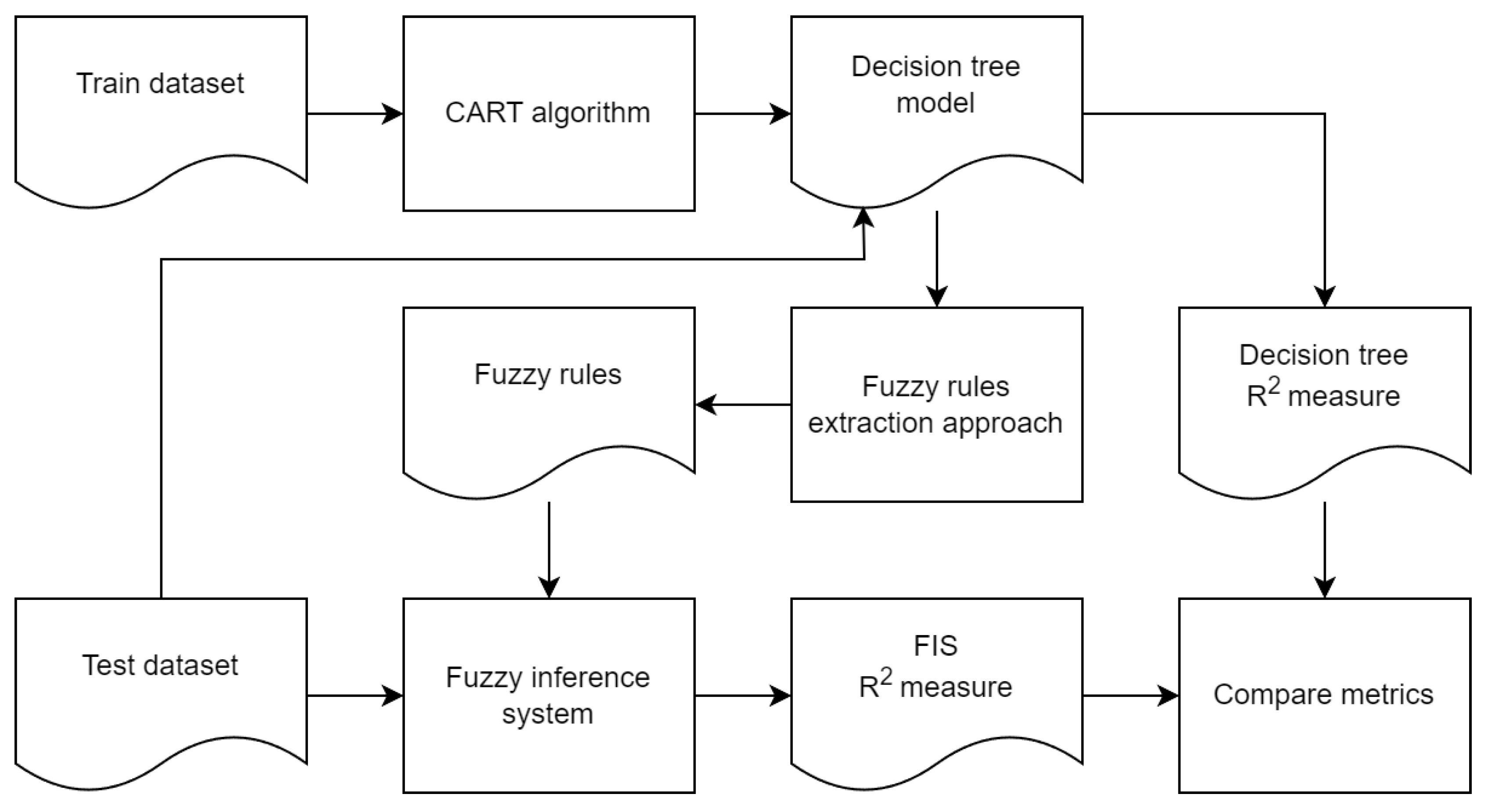
Figure 2.
Rule simplification schema
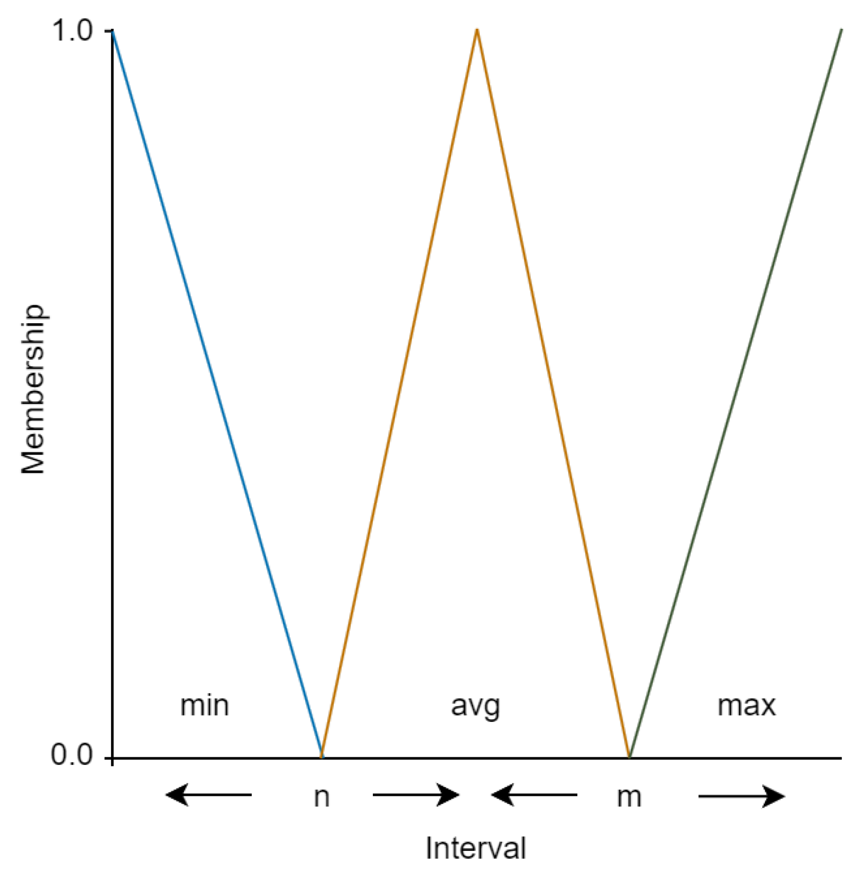
Figure 3.
Fuzzy variable with three linguistic terms

Figure 4.
Fuzzy variable with three linguistic terms
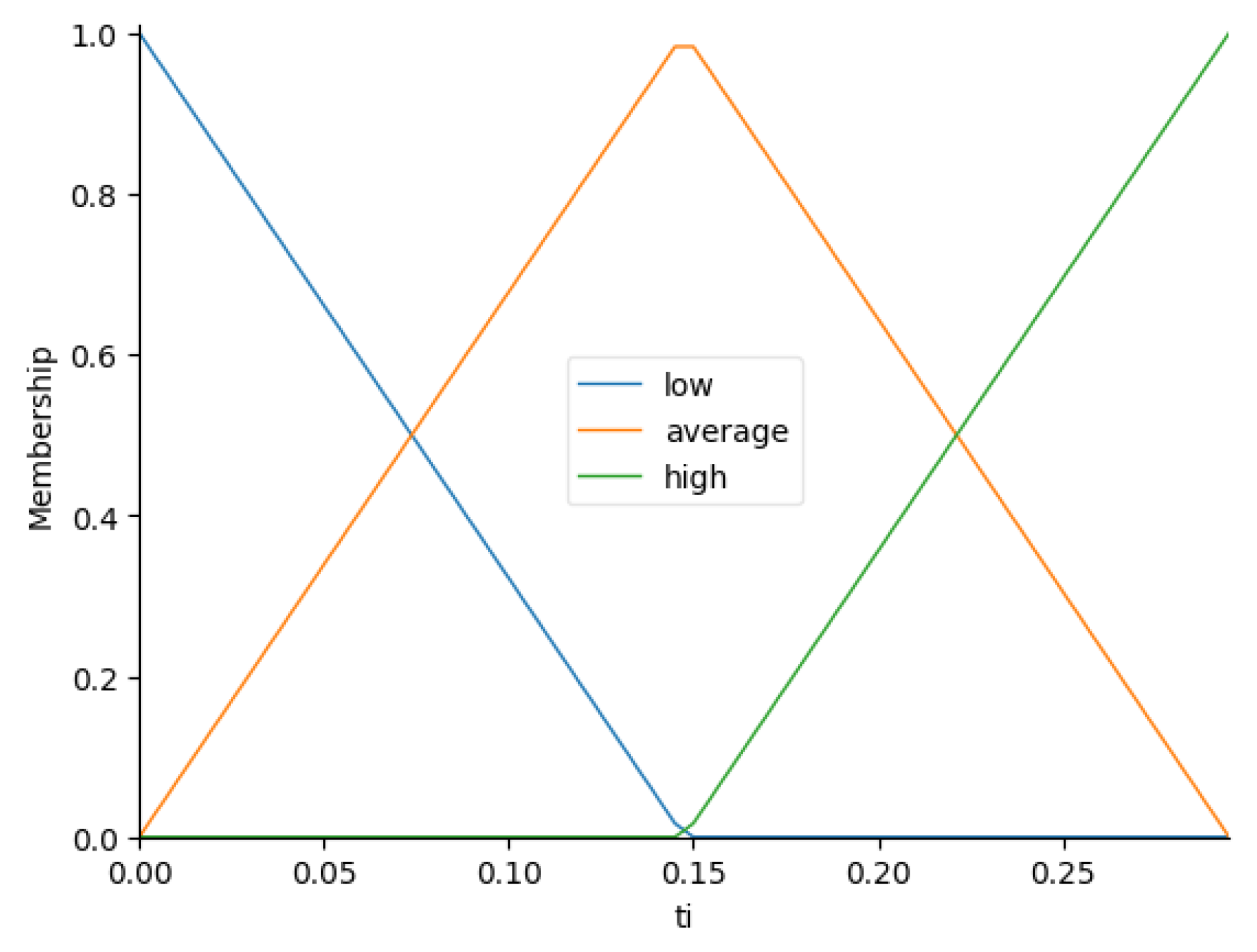
Figure 5.
Fuzzy variable with three linguistic terms
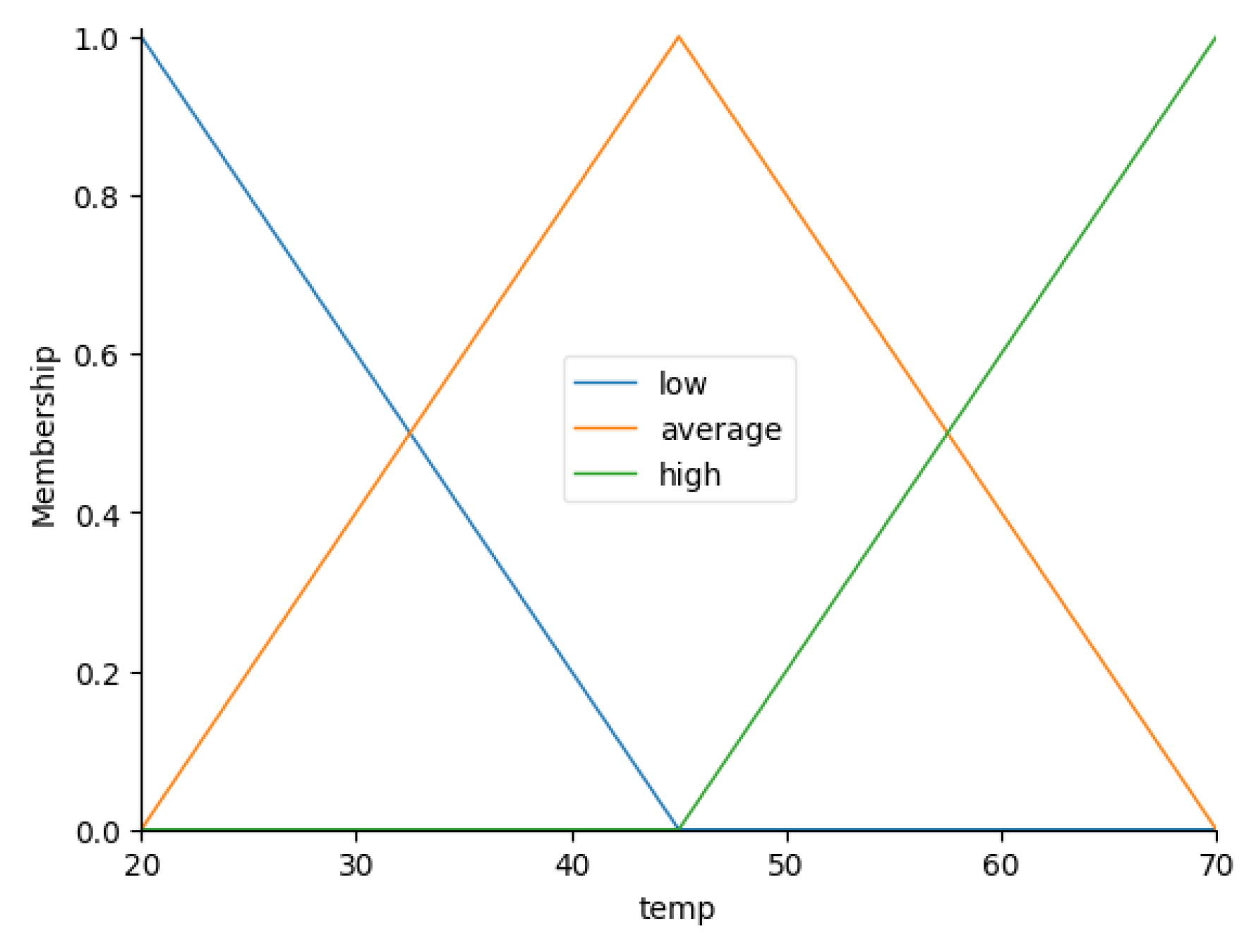
Figure 6.
Fuzzy variable with five linguistic terms
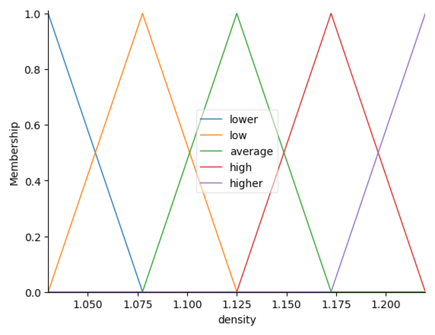
Figure 7.
Accumulation result for fuzzy variable
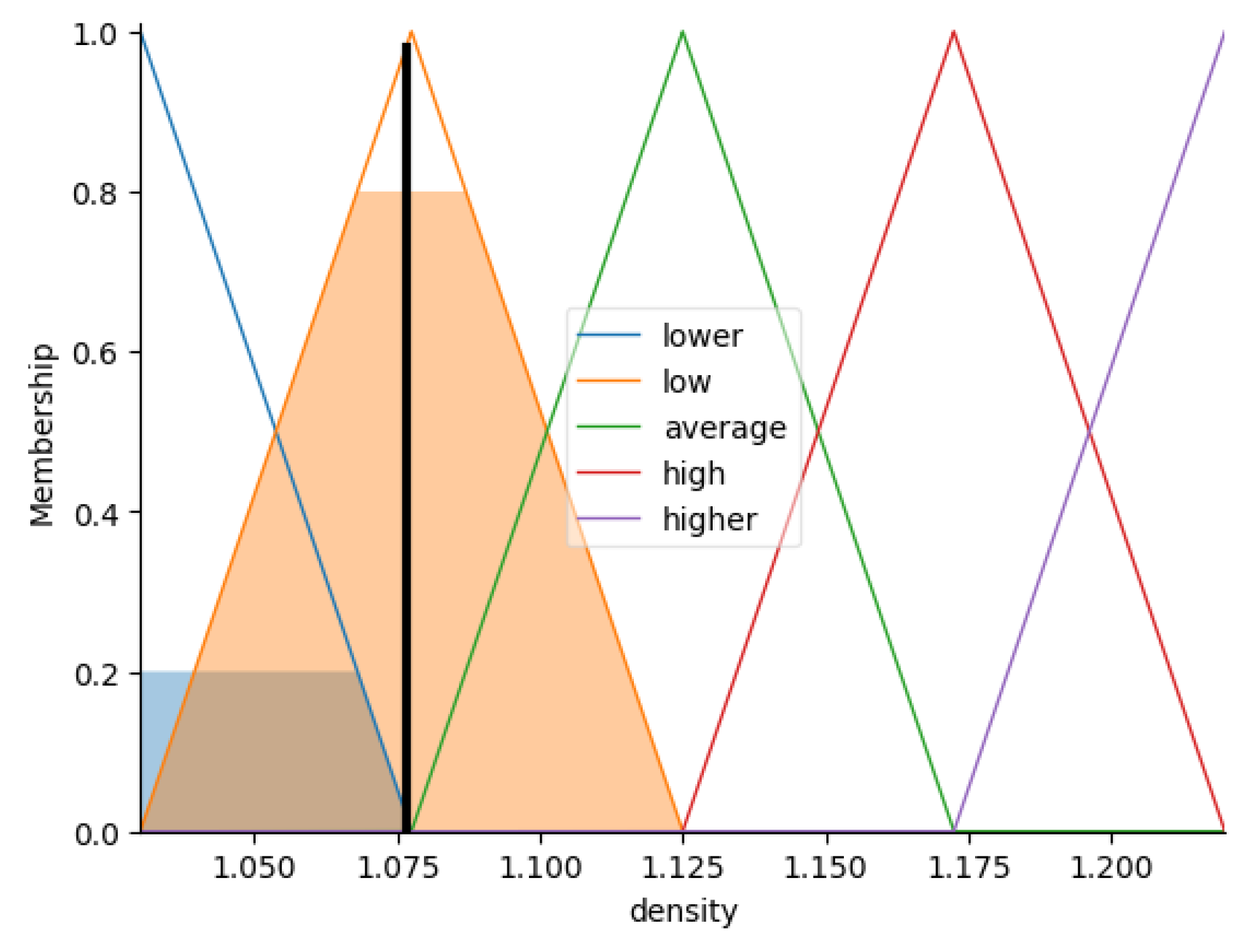
Figure 8.
Silhouette score diagram
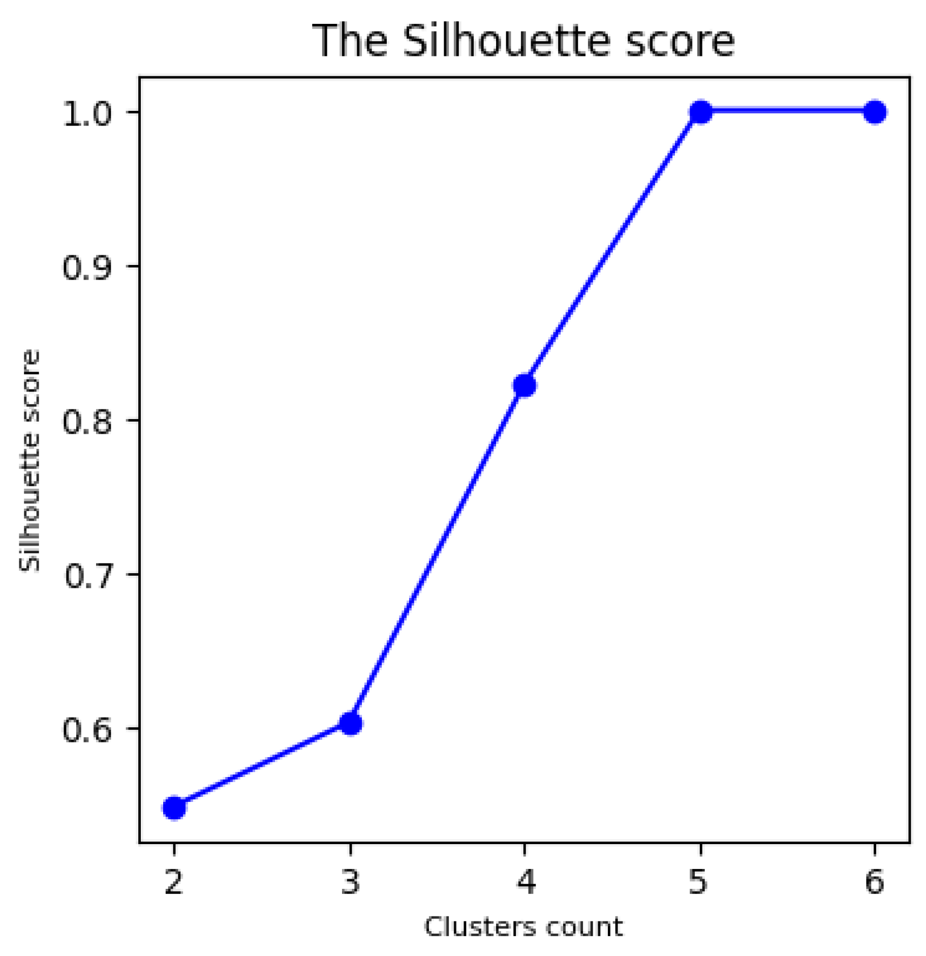
Figure 9.
Fuzzy variable with five linguistic terms
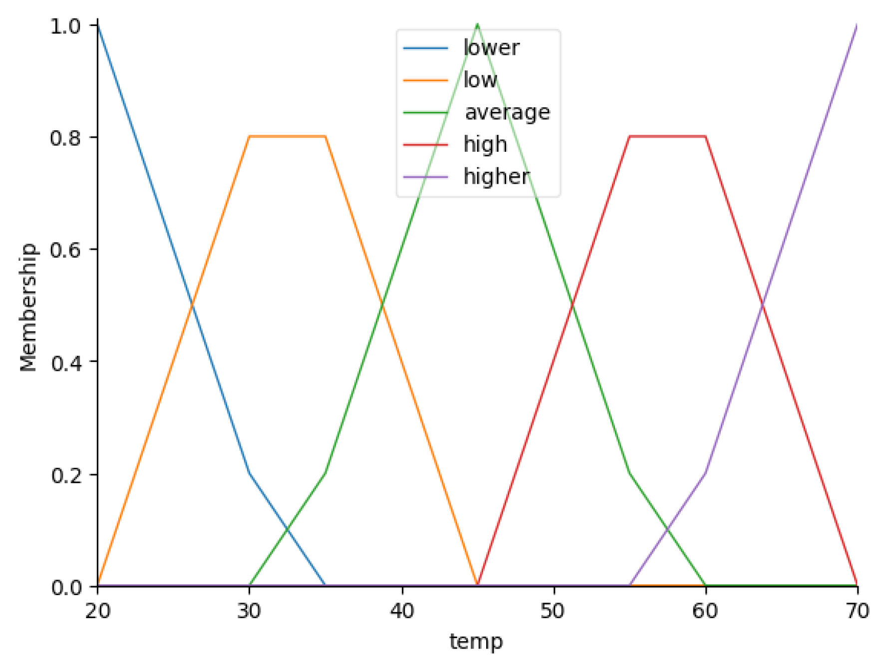
Figure 10.
Fuzzy variable with five linguistic terms
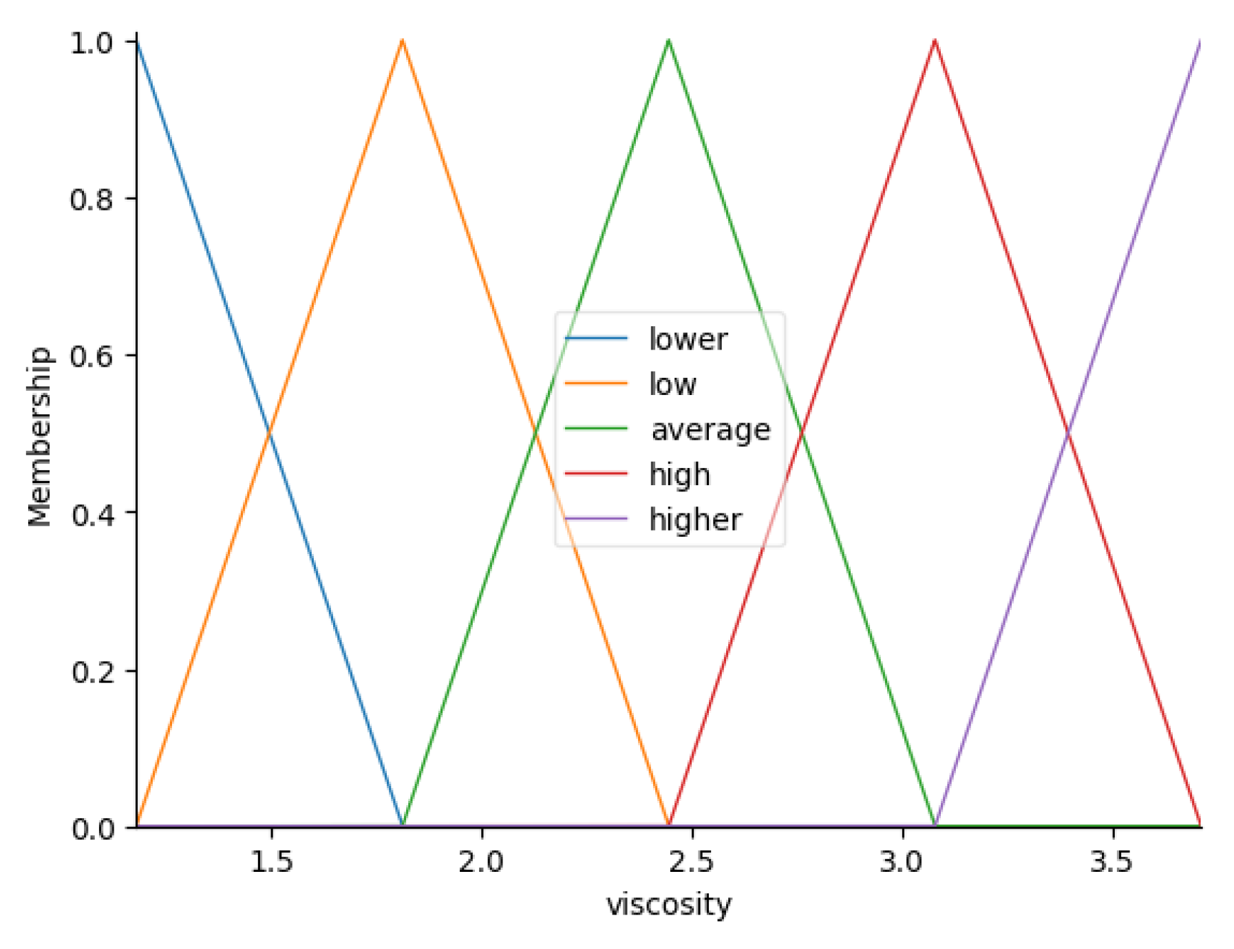
Table 1.
Experimental results
| # | (°C) | (%) | (%) | Real | Inferred | RMSE |
|---|---|---|---|---|---|---|
| 1 | 30 | 0 | 0 | 1.056 | 1.073 | 0.017 |
| 2 | 55 | 0 | 0 | 1.041 | 1.047 | 0.006 |
| 3 | 25 | 0.05 | 0 | 1.084 | 1.076 | 0.008 |
| 4 | 30 | 0.05 | 0 | 1.081 | 1.073 | 0.007 |
| 5 | 35 | 0.05 | 0 | 1.077 | 1.069 | 0.009 |
| 6 | 40 | 0.05 | 0 | 1.074 | 1.067 | 0.007 |
| 7 | 60 | 0.05 | 0 | 1.061 | 1.067 | 0.007 |
| 8 | 35 | 0.3 | 0 | 1.174 | 1.172 | 0.002 |
| 9 | 65 | 0.3 | 0 | 1.148 | 1.136 | 0.012 |
| 10 | 45 | 0 | 0.05 | 1.074 | 1.067 | 0.007 |
| 11 | 50 | 0 | 0.05 | 1.071 | 1.067 | 0.004 |
| 12 | 55 | 0 | 0.05 | 1.067 | 1.068 | 0.001 |
| 13 | 20 | 0 | 0.3 | 1.224 | 1.204 | 0.020 |
| 14 | 30 | 0 | 0.3 | 1.213 | 1.202 | 0.011 |
| 15 | 40 | 0 | 0.3 | 1.202 | 1.203 | 0.001 |
| 16 | 60 | 0 | 0.3 | 1.182 | 1.176 | 0.007 |
| 17 | 70 | 0 | 0.3 | 1.172 | 1.172 | 0.000 |
| Total | 0.009 | |||||
| 1 | 30 | 0 | 0 | 2.716 | 3.089 | 0.374 |
| 2 | 40 | 0 | 0 | 2.073 | 2.359 | 0.287 |
| 3 | 60 | 0 | 0 | 1.329 | 1.465 | 0.137 |
| 4 | 65 | 0 | 0 | 1.211 | 1.414 | 0.204 |
| 5 | 25 | 0.05 | 0 | 4.120 | 3.188 | 0.931 |
| 6 | 45 | 0.05 | 0 | 2.217 | 2.045 | 0.171 |
| 7 | 65 | 0.05 | 0 | 1.315 | 1.414 | 0.100 |
| 8 | 70 | 0.05 | 0 | 1.105 | 1.408 | 0.304 |
| 9 | 45 | 0.3 | 0 | 3.111 | 3.499 | 0.388 |
| 10 | 50 | 0.3 | 0 | 2.735 | 3.475 | 0.740 |
| 11 | 65 | 0.3 | 0 | 1.936 | 1.812 | 0.124 |
| 12 | 30 | 0 | 0.05 | 3.587 | 3.111 | 0.475 |
| 13 | 55 | 0 | 0.05 | 1.953 | 2.128 | 0.176 |
| 14 | 65 | 0 | 0.05 | 1.443 | 1.414 | 0.028 |
| 15 | 40 | 0 | 0.3 | 3.990 | 3.475 | 0.515 |
| 16 | 50 | 0 | 0.3 | 3.189 | 3.475 | 0.286 |
| 17 | 65 | 0 | 0.3 | 2.287 | 1.812 | 0.475 |
| Total | 0.407 | |||||
Disclaimer/Publisher’s Note: The statements, opinions and data contained in all publications are solely those of the individual author(s) and contributor(s) and not of MDPI and/or the editor(s). MDPI and/or the editor(s) disclaim responsibility for any injury to people or property resulting from any ideas, methods, instructions or products referred to in the content. |
© 2024 by the authors. Licensee MDPI, Basel, Switzerland. This article is an open access article distributed under the terms and conditions of the Creative Commons Attribution (CC BY) license (http://creativecommons.org/licenses/by/4.0/).
Copyright: This open access article is published under a Creative Commons CC BY 4.0 license, which permit the free download, distribution, and reuse, provided that the author and preprint are cited in any reuse.


