
Submitted:
13 August 2025
Posted:
14 August 2025
You are already at the latest version
Abstract
The paper presents a comprehensive MATLAB software package designed to model and solve a broad class of problems in fuzzy relational calculus: inverse problem for fuzzy linear systems of equations and fuzzy linear systems of inequalities; behaviour, reduction and minimization for finite fuzzy machines; optimization of linear objective function under fuzzy linear system of equations or inequalities constraints. The software supports a variety of fuzzy algebras, such as max−min, min−max, max−product, Goguen, Gödel, and Łukasiewicz, offering tools for direct and inverse problem resolution. The implementation is based on well-established theoretical results in fuzzy logic and fuzzy algebraic structures, providing a robust foundation for exact and efficient computation. We begin by outlying the mathematical background and the principles behind the implemented algorithms. The development history of the package is briefly reviewed to highlight the motivations and design choices. A selection of examples is presented to illustrate the use of the software in different problem settings. The package is freely available and has been downloaded over 2100 times from MATLAB File Exchange, indicating the interest in applying fuzzy relational methods in computational environments.
Keywords:
fuzzy relational calculus
; fuzzy linear systems of equations
; fuzzy linear systems of inequalities
; finite fuzzy machines
; optimization of linear objective function
; software for fuzzy relational calculus
1. Introduction
We present theory and software for fuzzy relational calculus (FRC) with applications in variety of areas. Attention is paid on the inverse problem resolution and obtaining complete solution set for fuzzy linear system of equations (FLSEs) and fuzzy linear system of inequalities (FLSIs). Applications are given for finite fuzzy machines – behaviour, reduction and minimization, as well as for optimization of linear objective function under FLSEs or FLSIs constraints.
Chronologically the main problem - how to solve FLSEs arose when we investigated finite fuzzy machines: in order to find finite behaviour matrix, to reduce or minimize states, we needed a solution method for FLSEs. This motivated our interest to FLSEs.
Publications for FLSEs demonstrate long period of investigations for discovering methods and procedures to solve them. Traditional linear algebra methods [1] cannot be used here – operations in fuzzy algebras are different from classical addition and multiplication.
A short review of the main results and approaches follows. Fuzzy relational equations (FREs) were first proposed in connection with medical diagnosis by Sanchez [2,3]. In [4] (1976) he gave formulas how to compute the maximal solution in the case of composition (Theorem 5) and the minimal solution in the case of composition (Theorem 6).
After Sanchez results attention was paid to the lower solutions of FLSEs, the complete solution set and the solution procedures. Higashi and Klir in [5] (1984) improved the results from Czogała et. all [6] (1982) and derived several schemes for solving finite FREs. assuming that the coefficients on the right-hind side of FLSEs are ordered decreasingly. The procedures are tremendous. Analogical approach was given by Miyakoshi and Shimbo [7] (1986), the results are valid for FREs with triangular norms. Pappis and Sugeno [8] (1985) proposed analytical method for obtaining the lower solutions, marking the essential coefficients for the solution and introducing the dominance condition (that helps to exclude from investigation some non-essential paths); nevertheless, the set of potential lower solutions has to be investigated in order to find valid one. Pappis and Adamopoulos [9,10,11], proposed procedures for inverse problem resolution in ZBasic for matrices with dimensions up to 10x10. Peeva [12] (1992) proposed analytical method and algorithms to solve FLSEs, introducing three semantic types of coefficients (G and E as essential and S as non-essential) for the potential solutions. She also marked that the time complexity of the algorithm for finding lower solutions is exponential, later proved by Chen and Wang [13] (2002).
After these early years the interest was paid to other compositions: (Peeva and Kyosev [15]); product (Bourke and Fisher [16], Di Nola et. all [17], Loetamonphong and Fang [18], Markovskii [19]); norm (Bartl and Belohlávek [20], Feng Sun [21], Nosková and Perfilieva [22]); residuum (Perfilieva and Nosková [23]), etc.
There exist many other valuable publications and generalizations for the inverse problem resolution: see Bartl as well as Bartl and co-authors [24–26]; De Baets [27]; Di Nola et. all [17]; Li and Fang [28]; Molai and Khorram [29]; Shieh [30]; Shivanian [31]; Wu and Guu [32].
Finding analytical method for the lower solutions is a long and arduous period [33], not to mention the even more difficult task of a software. The procedures are tremendous. The time complexity of the problem is exponential [13]. Various approaches were proposed to find solutions (extremal and the set of all solutions):
- characteristic matrix and decomposition [7,8];
- covering and binding variables [19,35–37];
- partitions and irreducible paths [5];
- solution based matrix [13], etc.
In this paper attention is paid on software description (based on our unified approach and exact methods) for solving FLSEs in somealgebras: in Gödel algebra, in Goguen algebra and in Łukasiewicz algebra.
In Section 2 we give the basic notions for the exposition - algebra, Gödel algebra, Goguen algebra and Łukasiewicz algebra, and norms, compositions of fuzzy relations and variety of products for finite fuzzy matrices.
Section 3 presents the theory and exact method for solving FLSEs or FLSIs in some algebras. A short overview is given of the chronological development of the fundamental ideas.
Applications for finite fuzzy machines and for linear optimization problems are subject of Section 4. They concern solving behaviour, reduction and minimization problems for finite fuzzy machines and solving linear optimization problems subject to FLSEs of FLSIs constraints.
The exact algorithms currently used in the software [38] are explained in details in Section 5, together with their computational complexity.
Section 6 presents the software from [38] itself and describes each of its modules and capabilities.
All algorithms and software functions are supported by examples provided in Appendix A.
2. Basic Notions
In this section the notions for classical algebra, orders and lattices are given according to [1,39], for algebra – according to [40], for fuzziness - according to [15].
Partial order relation on a partially ordered set (poset) P is denoted by the symbol ≤. By a greatest element of a poset P we mean an element such that for all . The least element of P is defined dually.
2.1. algebra
algebra is the algebraic structure:
where are binary operations, are constants and:
- is a lattice with universal bounds 0 and 1;
- is a commutative semigroup;
- * and → establish an adjoint couple:
- for all
We suppose in next exposition that and .
The following algebras are examples for algebras:
-
Gödel algebrawhere operations are
- (a)
- Maximum or conorm:
- (b)
- Minimum or norm:
- (c)
- The residuum is
- (d)
- A supplementary operation is useful
-
Product (Goguen) algebrawhere max and min are as (1) and (2), respectively, ∘ is the conventional real number multiplication (the norm, i. e, ) and the residuum isHere the supplementary useful operation is:
-
- (a)
- (b)
- The residuum is
- (c)
- A supplementary operation is useful
These operations, as well as the operations in Table 1 are realized in [38], see Section 5, Section 6, and Apendix Appendix A for details and working examples.
These three couples are also described as norms and norms (or conorms):
2.2. Compositions of Fuzzy Relations and Fuzzy Matrix Products
Let X and Y be crisp sets and denote all fuzzy sets over . A fuzzy relation is defined as a fuzzy subset of the Cartesian product ,
The inverse(or transpose) of is defined as
The finite fuzzy matrix (FFM) , with for each , , is called a membership matrix.
Any fuzzy relation over finite support is representable by FFM, written for convenience with the same letter , where for any .
The matrix representation of the inverse fuzzy relation is , called transpose or inverse of the given matrix. In this sense .
Two FFMs are called conformable, if the number of the columns in the first FFM equals the number of the rows in the second FFM: the matrices and are conformable and their product , in this order, makes sense.
We consider some products of FFMs in algebras. Since in references special attention is paid on , and compositions, they are specially listed in next Definition 1.
Definition 1.
Let and be conformable FFMs.
The FFM , where
- i)
- is called the product of A and B if
- ii)
- is called the product of A and B if
- iii)
- is called the product (the product ’.’ is the conventional real number multiplication) of A and B if
- iv)
- is called the product of A and B if
- v)
- is called the product of A and B if
- vi)
- is called the product of A and B if
For simplicity and compactness of exposition we write for any of the matrix products introduced in Definition 1.
Definition 2.
Let and be conformable FFMs. The matrix is called product of A and B in algebra, written , if for each , it holds:
where and are norm and norm respectively for , see Table 1.
2.3. Direct and inverse problem resolution
Let and be conformable FFMs. Computing their product according to Definition 1, 2 or 3, respectively, is called direct problem resolution.
Let Let and be given FFMs. Computing the matrix , such that or or is called inverse problem resolution.
Details for algorithm and software on this subject are given in subSection 5.1 and Section 6.2 with working examples in Appendix A.1.
3. FLSEs and FLSIs in Some Algebras
We began our investigations before 1992 [12] with , i.e. -norm FLSEs, given with long form and short form description:
Here stands for the matrix of coefficients, – for the matrix of unknowns, is the right-hand side of the system, , , for and
The next step was to investigate FLSEs and FLSEs . The main author’s results for all these FLSEs are published in [41].
The theoretical background - how to solve (11), is implemented as universal scheme in theory, algorithms and software for all the other kind of compositions for the FLSEs and FLSIs (, , as well as , , ), presented in the next subsection.
3.1. -norm FLSEs in algebras
The natural extension of the theory for FLSEs (11) leads to the unified approach for FLSEs when the composition is :
where is the matrix of coefficients, holds for the right-hand side vector, is the vector of unknowns; for the indices we suppose , ; are given, marks the unknowns in the system and () is according to Table 1.
The approach is also valid for FLSEs .
In the next exposition we suppose that the matrices A, X and B are as follows: , and .
3.2. Solutions
For FFMs and the inequality
means for each , .
Definition 4.
For the FLSEs (12) :
- i)
- is called a point solution of if holds.
- ii)
- iii)
- A solution is called an upper or maximal solution of (12) if for any the relation implies . When the upper solution is unique, it is called the greatest or maximumsolution .
- iv)
- A solution is called a lower or minimal solution of (12) if for any the relation implies . When the lower solution is unique, it is called the least or minimum solution .
- v)
- with for each j, , is called an interval solution if any belongs to when for each j, .
- vi)
- Any interval solution, whose interval bounds are bounded by a lower solution from the left and by the greatest solution from the right, is called maximal interval solution .
3.3. Solvability and greatest solution
We give the analytical expression for the greatest solution of FLSEs (12) and a criterion for its consistency.
Theorem 1.
[14] Let A and B be FFMs and let be the complete solution set of . Then:
- i)
- ;
- ii)
- If the FLSEs (12) is consistent, then is its greatest solution.
- iii)
- There exists polynomial time algorithm for computing .
Corollary 1.
[14] The following statements are valid for FLSEs :
In fact, Theorem 1, item ii), gives the analytical expression for the greatest solution of the equation (12). It is the core of the algorithms and software presented in [38] for establishing consistency of FLSEs and finding its extremal solution: maximum for the equation (12) and minimum for the dual case.
First we present finding the greatest solution of FLSEs (12) , a criterion for its consistency and and how to find the lower solutions, based on [42].
3.4. Greatest Solution
According to Theorem 1 any solvable -norm FLSEs has unique greatest solution. In order to find all solutions of the consistent system, it is necessary to find its greatest solution and all of its minimal solutions. Finding the greatest solution is relatively simple task which can be used as a criteria for establishing consistency of the system. Finding all minimal solutions is reasonable for consistent system.
3.4.1. Classical Approach
The approach how to solve (12) is based on Theorem 1 and Corollary 1.
If (12) is consistent, its greatest solution is .
Using this fact, an appropriate algorithm for checking consistency of the system and for finding its greatest solution can be obtained. Its computational complexity is . Nevertheless that it is simple, it is too hard for such a task.
3.4.2. More Efficient Approach
Here we propose a simpler way to answer both questions for (12) – consistency and the greatest solution (simultaneously computing the greatest solution and establishing consistency of (12)). Extending the ideas of [12] and [15], we work with four types of coefficients (S, E, G and H) and a boolean vector (IND).
In the FLSEs (12):
-
If i.e. operation is minimum ():
- −
- is called S-type coefficient if .
- −
- is called E-type coefficient if .
- −
- is called G-type coefficient if .
- −
- is called H-type coefficient if .
-
If i.e. operation is the algebraic product ():
- −
- is called S-type coefficient if .
- −
- is called E-type coefficient if .
- −
- is called G-type coefficient if .
- −
- is called H-type coefficient if .
-
If i.e. operation is the ukasiewicz norm ():
- −
- is called S-type coefficient if .
- −
- is called E-type coefficient if .
- −
- is called G-type coefficient if .
- −
- is called H-type coefficient if .
The next Algorithm 1 uses the fact that it is possible to find the value of the unknown only by the column of the matrix A. For every and depending on the operation, we consider the following cases:
-
When the operation is
- −
- If is E-type coefficient then the i-th equation can be satisfied by when because .
- −
- If is G-type coefficient then the i-th equation can be satisfied by only when because .
- −
- If is S-type coefficient then the i-th equation cannot be satisfied by for any .
-
When the operation is
- −
- If is E-type coefficient then the i-th equation can be satisfied by when because .
- −
- If is G-type coefficient then the i-th equation can be satisfied by only when because .
- −
- If is S-type coefficient then the i-th equation cannot be satisfied by for any .
-
When the operation is
- −
- If is E-type coefficient then the i-th equation can be satisfied by when because .
- −
- If is H-type coefficient then the i-th equation can be satisfied by only when because .
- −
- If is S-type coefficient then the i-th equation cannot be satisfied by for any .
Hence, S-type coefficients are not interesting because they do not lead to solution.
For the purposes of the next theorem, is introduced as follows:
- If the operation is :
- If the operation is :
- If the operation is :
Theorem 2.
[42] The FLSEs (12) is consistent iff is its solution.
Corollary 2.
[42] In a consistent FLSEs (12):
- choosing for at least one makes the system inconsistent;
- for every , the greatest admissible value for is ;
- its greatest solution is , .
In general, Theorem 2 and its Corollary show that instead of calculating we can implement a faster way to obtain (as realized in Algorithm 1).
is only the eventual greatest solution of the FLSEs (12) and it can be obtained for any FLSEs, even if the system is inconsistent, so the eventual solution should be checked in order to confirm that it is a solution of (12). Explicit checking for the eventual solution will increase the computational complexity of the algorithm. To avoid this in the next presented Algorithm 1 this is done by extraction of the coefficients of the potential greatest solution. For every we check which equations of (12) are satisfied (hold in the boolean vector ). If at the end of the algorithm all the equations of FLSEs (12) are satisfied (i.e. all the coefficients in are set to ) this means that the system is consistent and the computed solution is its greatest solution, otherwise the FLSEs (12) is inconsistent.
| Algorithm 1 Greatest solution and consistency of FLSEs (12). |
|
Theorem 2 and its Corollary provide that if (12) is consistent, computed by Algorithm 1 is its greatest solution.
Algorithm 1 uses vector to check which equations are satisfied by the eventual . At the end of the algorithm if all components in are then is the greatest solution of the system, otherwise the system is inconsistent.
3.5. Lower Solutions
Each equation in (12) can be satisfied only by the terms with H-type coefficients. Also, the minimal value for every component in the solution is either the value of the corresponding or 0. Along these lines, the hearth of the presented here algorithm is to find H-type components in A and to give to either the value of the corresponding when the coefficient contributes to solve the system or 0 when it doesn’t.
Using this, the set of candidates for solutions can be obtained. All candidate solutions are of three different types:
- Lower solution;
- Non-lower solution;
- Not solution at all.
The aim of the next Algorithm 2 is to extract all lower solutions and to skip the second and third types (non-lower solution or not solution at all). In order to extract all lower solutions a method, based on the idea of the dominance matrix in combination with list manipulation techniques is developed here.
3.5.1. Domination
For the purposes of presented here Algorithm 2, the definition for domination is given.
Definition 5.
Let and be the and the equations, respectively, in (12) and . Equation is called dominant to and equation is called dominated by , if for each it holds: if is H-type coefficient then is also H-type coefficient.
3.5.2. Extracting Lower Solutions
Lower solutions are extracted by removing from A the dominated rows. A new matrix is produced and marked with where , for obvious reasons. It preserves all the needed information from A to obtain the solutions.
Extraction introduced here is based on the following recursive principle. If in the column of there are one or more rows () such that coefficients are H-type then should be taken equal to the smallest and all rows should be removed from . The same procedure is repeated for column of the reduced . "Backtracking" based algorithm using this principle is presented next:
| Algorithm 2 Extract the lower solutions from . |
|
3.6. General algorithm
The next algorithm is based on the above given Algorithms 1 and 2.
| Algorithm 3 Solving . |
|
Algorithm 2 (Step 5) is the slowest part of the Algorithm 3. In general this algorithm has its best and worst cases and this is the most important improvement according to algebraic-logical approach [41] (from the time complexity point of view). Algorithm 2 is going to have the same time complexity as the algorithm presented in [14] only in its worst case.
Concerning the FLSEs - this is the analogical case and we do not describe the theory here, but software is also available in [38].
More details for algorithms and software for all of the main problems in this section are given in subSection 5.2 and Section 6.3 with working examples in Apendix Appendix A.2.
Software for inverse problem resolution is provided in [34] (only for and FLSEs) and in [38] for all other cases.
3.7. -Norm FLSIs in Algebras
For the FLSIs , , , , we implement analogical approach as described for the FLSEs .
For algorithms and software for FLSIs see also subSection 5.4, Section 5.5 and Section 6.3 with working examples in Apendix Appendix A.2.
3.8. Short Chronological Overview
The historical core of these methods was the algebraic-logical approach [12,14,15,41] which is still the main basis of all the currently used algorithms. This approach introduced a structured methodology involving potential extremal solutions, consistency checks via index vectors, and coefficient classification. The coefficients in the matrix of the coefficients A were categorized into three semantic types : S-type, E-type, and G-type coefficients [12,15]. A later refinement introduced H-type coefficients [41], which acted as a lightweight abstraction to further streamline certain matrix operations without changing the semantic interpretation of the system.
Such classifications made it possible to construct associated matrix [12] that was used to generate solution intervals and identify dominating paths. The dominance relation [41] was fundamental for reducing complexity by pruning branches that could not lead to solutions.
The next fundamental step is the construction of so-called help matrix [15], used to guide the recursive generation of candidate solutions. In some algorithmic versions, these structures were complemented by list-based procedures, where possible solutions and operations were represented and manipulated as lists rather than fixed-size matrices. These list-based algorithms enabled greater flexibility in traversing the solutions, but turn out to be even more complex from implementational point of view. Although the computational complexity of this problem is exponential [13], various simplification heuristics were developed to make the process more tractable in practice.
Over time, these methods evolved and expanded to support a wide variety of compositions in BL-algebras, including not only max–min but also , max-product, and other BL systems such as those using the Goguen or Łukasiewicz implications. [42–44]. New versions of the algorithms integrated modular procedures that preserved the core logical structure while allowing extensibility to different algebras.
It is worth mentioning that the current implementation still employs a structure referred to as the help matrix, although its construction and role have significantly changed. The current algorithmic flow is explained in Section 5.
The evolution of these methods and their application to broader classes of fuzzy systems is documented in a series of publications [42–44]. These works include concrete examples and software implementations. Although the internal architecture of the software has shifted toward more unified and abstract representations (as detailed in Section 6), many of the core ideas — such as the use of coefficient classification, list-based construction, and filtering - continue to influence the current implementation.
4. Some Applications
4.1. Linear Dependency/Independency
Let , be fuzzy column-vectors with elements for , .
The fuzzy column-vector is called linear combination of if there exist such that Checking whether is a linear combination of requires to solve the system (12)
for the unknown X, if has as columns ,
If the FLSEs is consistent the vectors are linearly dependent. When the FLSEs is inconsistent, the vectors are linearly independent.
We implement this for instance in subSection 4.2 for finite fuzzy machines when computing the finite behaviour matrix, as well as for minimization of states.
The algorithms in subSection 5.6 and Section 5.7 are for establishing linear combination as well as linear dependency/independency. Software is described in subSection 6.2. Examples are given in Appendix A.1.
4.2. Finite Fuzzy Machines
We present finite fuzzy machines (FFMachs) with emphasis on the complete behavior matrix, reduction and minimization problems. For solving all these problems we implement the software from [38],
FFMachs were introduced by Santos, see [45] – 47]. Here the presentation is based on our results as published in [15,48].
For a finite set C we denote by its cardinality.
Definition 6.
A finite fuzzy machine is a quadruple
where:
- i)
- are nonempty finite sets of input letters, states and output letters, respectively.
- ii)
- is the set of transition-output matrices of , that determines its stepwise behavior. Each matrix is a square matrix of order and
In Definition 6 ii) we mark by the pair to emphasize that is the input letter when is the output response letter. The same stipulation is used in next exposition for input-output pair of words of the same length.
We regard as the degree of membership for the FFMach to enter state and produce output if the present state is and the input is .
4.2.1. Extended input-output behavior
While is the set of transition-output matrices that describes operating of for exactly one step, in this subsection we will be interested in matrices that describe operating of for input-output pairs of words.
The free monoid of the words over the finite set X is denoted by with the empty worde as the identity element. If then is countably infinite. The length of the word u is denoted by . By definition . Obviously for each , stands for the set of natural numbers.
For and , if we write to distinguish it from the case . We denote by the set of all input-output pairs of words of the same length:
Definition 7.
Let be FFMach.
For any the extended input-output behavior of upon the law of composition * is determined by the square matrix of order :
where , for , or products and is the square matrix of order with elements determined as follows:
- if the composition is or product,
- if the composition is ,
Each element in is the degree of membership that will enter state and produce output word under the input word beginning at state , after consecutive steps.
Definition 7 describes the extended input-output behavior of , and product FFMachs.
4.2.2. Complete input-output behavior
When we consider FFMach as a ’black box’ we are not interested in the next state . This is the essence of the input-output behavior of , determined by column-matrices as follows:
where E is the column-matrix with all elements equal to 1 if the composition is or product and with all elements equal to 0 if the composition is .
Each element of in (17) determines the operation of under the input word u beginning at state q and producing the output word v after consecutive steps.
For instance, if the FFMach is or product, the element
gives the way of achieving maximal degree of membership under the input word u, beginning at state q and producing the output word v.
We denote by the complete behavior matrix of . It is semi-infinite matrix with rows and with columns , computed by (17) and ordered according to the lexicographical order in , see Table 2.
Let us mention that for if FFMach is or product, for if FFMach is
4.3. Behavior Matrix
For any FFMach its complete input-output behavior matrix is semi-infinite – it has finite number of rows (equal to the number of states in Q) and infinite number of columns. Since is semi-infinite, one can not solve traditional problems – equivalence of states, reduction of states, minimization of states, because all of them explore .
The matrix obtained by omitting all columns from that are linear combination of the previous columns is called behavior matrix of .
We may compute the behaviour matrix for FFMach, but the time complexity of the algorithm is exponential. Algorithm 15 in subSection 5.8 extracts the finite behaviour matrix from the complete behavior matrix , it implements linear dependency/independency from subSection 4.1.
4.4. Equivalence of States, Reduction, Minimization
captures all the properties of and provides solving equivalence, reduction and minimization problems for FFMachs.
For the FFMach the states and are called equivalent if the input-output behavior of when beginning with initial state is the same as its input-output behavior when beginning with initial state It means that the th and th rows are identical in and in . Since is semi-infinite, we can not derive equivalence of states from it. In order to solve this problem we first have to extract from and then to find identical rows in . Then we left only one of those identical rows.
FFMach is in reduced form if there does not exist equivalent states in Q.
A FFMach is not in minimal form if the input-output behavior of when it begins with initial state is the same as its input-output behavior when it begins with initial distribution over Q, isolating the state Formally it means that the th row of (, respectively) is a linear combination of the other rows.
Software from [38] implements this idea: if the th row of is a linear combination of the other rows of , then the FFMach is not in minimal form.
Algorithms and software for obtaining the behaviour matrix, as well as for solving reduction and minimization problems are given in subSection 5.8 and Section 6.4 with working examples in Appendix A.3.
4.5. Linear Optimization
We present optimization problem when the linear objective function is
with traditional addition and multiplication; is the weight (cost) vector and the function (18) is subject to FLSEs or FLSIs as constraint
The aim is to minimize or maximize Z subject to one of the constraints in (19).
The linear optimization problem was investigated first for composition by Fang and Li [49], Guu and Wu [50], Peeva [41]; for product composition by Loetamphong and Fang [51], Peeva and co-authors [52]; for algebras by Peeva and Petrov [53]. If the objective function becomes with the so called latticized linear programming problem was studied by Wang et al [54].
Since the solution set of (19) is non-convex, traditional linear programming methods cannot be applied. In order to find the optimal solution for (18), the problem is converted into a integer programming problem. Fang and Li in [49] solved this integer programming problem by branch and bound method with jump-tracking technique. Improvements of this method are proposed in [55] by providing fixed initial upper bound for the branch and bound part and with update of this initial upper bound. Conventional investigations [49], [50], [51], [55] begin with various attempts to find some feasible solutions, then to find an arbitrary solution of the optimization problem subject to constraint from (19) and proceed with it in the solution set for search of minimal solutions. The procedures are clumsy, the main obstacle is how to solve (19).
The algorithms and software from [38] proceeds for solving optimization problems, among them are:
- i)
- Minimize the linear objective function (18), subject to FLSEs constraints, when the composition is , product or ukasiewicz;
- ii)
- Maximize the linear objective function (18), subject to FLSEs, when the composition is , product or ukasiewicz;
- iii)
- Minimize or maximize the linear objective function (18), subject to FLSEs constraints, when the composition is
For clarity of exposition we present the ideas for and product case.
4.6. Minimize the Linear Objective Function, Subject to FLSEs Constraints, When the Composition is or Product Case.
We present how to minimize the linear objective function (18), subject to constraints: a fuzzy linear system of equations with or product composition
where with stands for the matrix of coefficients, , stands for the matrix of unknowns, , is the right-hand side of the system, the or product composition is written as ∘ and is the weight (cost) vector.
We apply the software from [38] for computing the greatest solution and all minimal solutions of the consistent system . Then we solve the linear optimization problem, first decomposing Z into two vectors and , such that and:
4.7. Maximize the Linear Objective Function, Subject to Constraints , When the Composition is or Product
4.8. Algorithm for Finding Optimal Solutions
We propose the algorithm for finding optimal solutions if the linear objective function is Z and the composition is or product for the constraints (20).
In any of these cases the optimal value is
The algorithm for finding optimal solutions is based on the above results.
| Algorithm 4 Algorithm for finding optimal solutions |
|
Algorithms and software for the above described linear optimization problems are given in subSection 5.9 and Section 6.5 with working examples in Appendix A.4.
5. Algorithms
In this section, we present algorithms that have been developed over the years and are used in the software [38]. These algorithms cover fuzzy matrix compositions, inverse problem resolution, linear dependence and independence, fuzzy optimization, and finite fuzzy machines. They are designed to support a variety of fuzzy algebras, including max-min, min-max, max-product, and all the others defined in Definitions 1 - 3.
However, in order to keep the exposition focused and accessible, we restrict attention in this chapter to the max-min case. This is justified not only by its historical role in the development of fuzzy relational methods, but also by the fact that it forms the basis of many practical applications. Other compositions introduced in Definitions 1 - 3 will be demonstrated in the following Chapter Section 6.
The inverse problem for fuzzy linear systems is particularly challenging when computing the complete solution set. The algorithms presented here incorporate structural optimizations to address this challenge while preserving the mathematical properties of the underlying systems.
5.1. Fuzzy Matrix Compositions
Direct problem in FRC means fuzzy matrix composition. According to Definitions 1 - 3, fuzzy matrix composition is defined by applying two fuzzy operations. Similarly to conventional matrix multiplication, the general procedure computes each entry of the resulting matrix C from the row i of matrix A and column j of matrix B.
Complexity: Algorithm 5 computes each entry by evaluating k pairs and aggregating the result, leading to a total of basic operations. This gives a complexity of .
| Algorithm 5 Generic Fuzzy Matrix Composition |
|
This algorithm serves as a general template for all supported compositions. Each specific case, such as max-min, min-max, max-product, or compositions based on fuzzy implications is implemented as an alias function that calls this general routine with the corresponding pair of fuzzy operations.
5.2. Inverse Problem Resolution for Fuzzy Linear Systems of Equations
The inverse problem in FRC consists of solving an FLSEs of the form or or where A and B are known fuzzy matrices, X is the unknown, and the composition is defined as in Definitions 1 - 3. Solving this problem means finding the complete solution set under the selected fuzzy composition.
While direct composition is computationally straightforward, solving the inverse problem, especially for obtaining the complete solution set, is significantly more complex. In what follows, we focus on the classical case of max-min composition, where most theoretical and algorithmic developments are concentrated.
Over the years, several different algorithms have been developed and implemented for solving the inverse problem in Fuzzy Calculus Core. These earlier methods, based on the algebraic-logical framework and analytical constructions, are described in detail in Section 3. The current version of the software incorporates an optimized algorithm that builds on these foundational techniques.
The method described below represents the latest and most efficient version currently implemented in the software. It is designed to compute the greatest solution and recursively generate all minimal solutions through domination and recursive search.
Algorithm Overview
The algorithm for solving FLSEs under max-min composition is divided into the following stages:
- Stage 1: Initializations
- Stage 2: Find the greatest solution
- Stage 3: Domination
- Stage 4: Recursive extraction of all lower solutions
Stage 1: Initializations
| Algorithm 6 Stage 1: Initializations |
|
Stage 2: Find the greatest solution
Earlier algorithms for computing the greatest solution relied on slow residuum-based expressions or complicated algorithms based on S, E, G, and H elements, presented in Section 3.4.
The current implementation avoids implication operators entirely. Instead, it computes the greatest solution directly from the help matrix using column operations. The consistency of the system is checked during the same pass, marking all covered rows without additional matrix traversal. This leads to a significant improvement in performance and simplicity.
Complexity: Algorithm 7 requires at most comparisons in its worst-case scenario, giving complexity. This algorithm has better scenarios, where the solution can be found early for each variable, resulting in the best-case performance of .
| Algorithm 7 Stage 2: Find the greatest solution |
|
Stage 3: Domination
Definition 8.
[15] Let and be the th and the th rows, respectively, in the help matrix H. If for each j, , , then:
- is said to be a dominant row to in H
- is redundant row and can be removed from H
In earlier implementations, dominance was analyzed using a separate dominance matrix. In the current version, this step is evaluated directly over the help matrix.
Complexity: Algorithm 8 is giving a worst-case complexity of . In favorable cases where domination is detected early, many comparisons are skipped via early termination, resulting in best-case performance of .
| Algorithm 8 Stage 3: Domination |
|
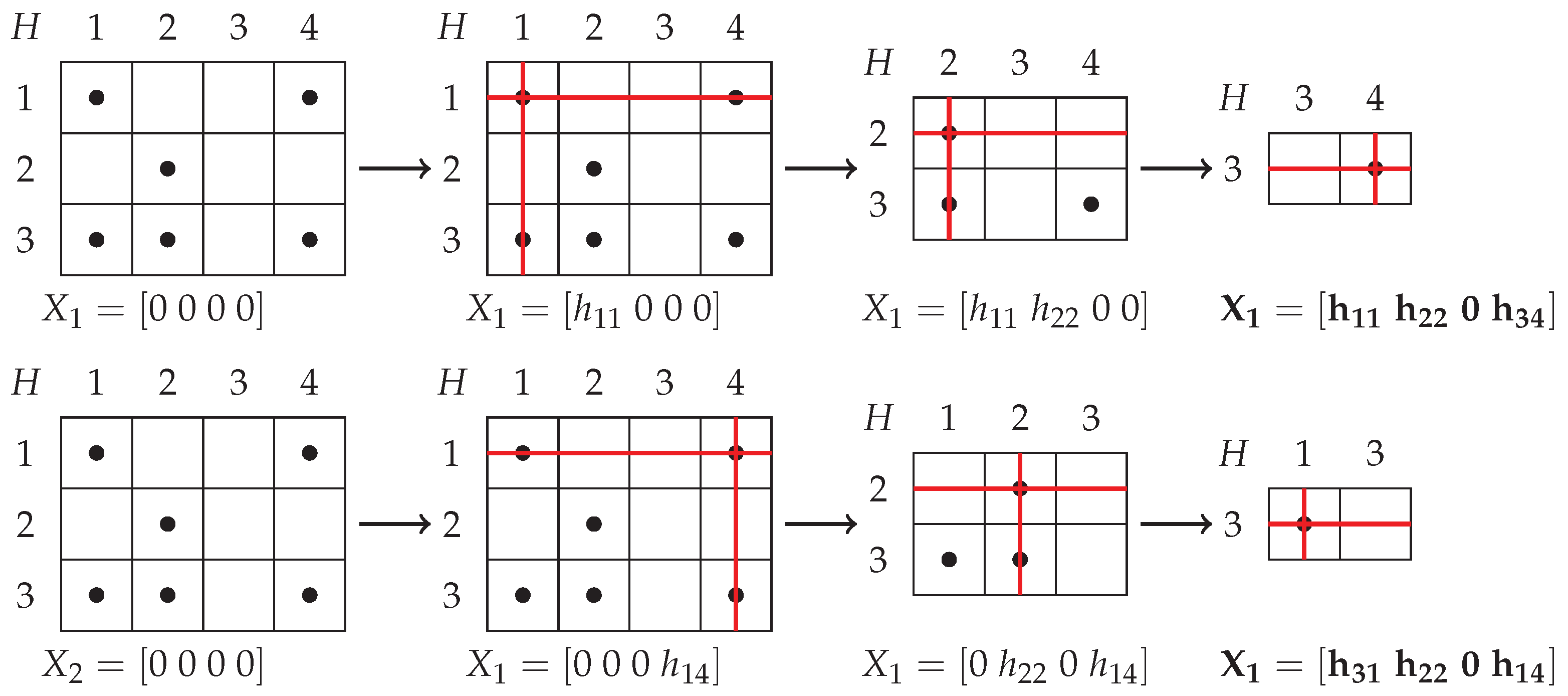
Stage 4: Recursive extraction of all lower solutions
The current implementation uses a recursive procedure that incrementally builds each solution from valid components in the help matrix. At every step, the algorithm maintains a set of uncovered rows and explores only those elements that contribute to the current potential solution. Branches that cannot lead to a complete solution are skipped early. This method avoids full enumeration of all combinations, and provides a conceptually simpler and more memory-efficient procedure.
 Complexity: The time complexity of the recursive extraction of all lower solutions from H is exponential, but in this case, it depends on the number of non-zero elements in the help matrix, which itself reflects the number of possible lower solutions. More precisely, in the worst case, the number of recursive paths can grow to , where d is the average number of non-zero entries per row, and m is the number of rows in H which may be smaller than in A, due to the domination step. In practice, however, the algorithm is highly efficient due to early pruning of incomplete branches and the reduced size of H after domination.
| Algorithm 9 Stage 4: Recursive extraction of all lower solutions |
|
Figure 1.
Visual representation of Algorithm 9.
5.3. Complete Algorithm for Solving
The previous procedures are combined into a complete algorithm for solving FLSEs .
Complexity: The total complexity is dominated by the recursive enumeration of all lower solutions (Algorithm 9), which is exponential in the number of rows in the help matrix. All preceding steps—help matrix construction, consistency check, and row domination—run in or time.
| Algorithm 10 Solving the inverse problem for |
|
The presented algorithm can be extended to other types of systems and compositions. Similar procedures are implemented in [38] for all composition operators defined in Definition 1, illustrating the potential for both algorithmic and theoretical generalizations of this approach.
5.4. Inverse Problem Resolution for Fuzzy Linear Systems of ≥ Inequalities
While FLSEs of the form have been widely studied, FLSIs such as have received comparatively little attention in the literature. To the best of our knowledge, no other general-purpose software tools for solving such systems exist.
The algorithms presented in the previous section for solving FLSEs can be extended to handle systems of inequalities with only minor modifications. In this section, we focus on the case , where the greatest solution is trivial if it exists, but lower solutions must still be extracted recursively. We cannot assume that the corresponding system of equations has a solution, there are cases where the inequality system is consistent, even though the equation system is not. We highlight the key differences in structure and interpretation compared to the case of equations.
Complexity: The computational complexity is identical to that of the algorithms described in Section 5.2.
| Algorithm 11 Solving the inverse problem for |
|
5.5. Inverse Problem Resolution for Fuzzy Linear Systems of ≤ Inequalities
FLSIs of the form are structurally simpler than equations or ≥ inequalities. A trivial lower solution X of all zeros always exists, and no recursive extraction is required. The problem reduces to finding the greatest solution that satisfies all inequality constraints. This is performed using the same method as in the equality case, with minor simplifications.
Complexity: The complexity is significantly lower than in Section 6.2. No domination or recursion is required. We are left with just the greatest solution, which is computed in time.
| Algorithm 12 Solving the inverse problem for |
|
5.6. Fuzzy Linear Combination of Vectors
A fuzzy vector B is said to be a linear combination of the columns of a matrix A under a fixed composition (e.g. max-min) if there exists a fuzzy vector X such that . This is equivalent to solving the inverse problem.
To determine whether such a combination exists, we reuse the algorithms for computing the greatest solution described in Section 5.2. Since we are only interested in the existence of a solution, it is sufficient to validate that the system is consistent i.e. there is no need to extract all lower solutions.
Complexity: The complexity is the same as the consistency check in Algorithm 7.
| Algorithm 13 Check if B is a fuzzy linear combination of the columns of A |
|
5.7. Fuzzy Linear Independence
A set of fuzzy vectors is said to be linearly independent if no vector in the set can be expressed as a fuzzy linear combination of the others vectors under a fixed composition (e.g. max-min).
Our implementation tests linear independence by iteratively checking, each column in a fuzzy matrix A, for a linear combination of the remaining columns. This is done using the procedure from Algorithm 13.
Complexity: The algorithm performs n consistency checks, each with complexity . Therefore, the total complexity is .
| Algorithm 14 Check if the columns of A are fuzzy linearly independent |
|
5.8. Finite Fuzzy Machines
This subsection focuses on computing the behavior of max-min FFMach, see subSection 4.2. The behavior matrix is obtained by composing all reachable transitions iteratively until stabilization. The process terminates automatically when further compositions no longer change the result.
Here we present the algorithms used in [38] for computing the behavior matrix, and for two types of postprocessing: reduction and minimization presented in Section 4.2.
Complexity: Let N denote the final number of behavioral vectors in the matrix B. At each iteration, up to new candidates are generated, where k is the number of fuzzy transition matrices and n is the current number of columns in B. Each new vector is tested for fuzzy linear combination against the existing ones, using Algorithm 13, which has complexity for vectors of length m. Assuming no vector is rejected as dependent, the total number of candidates grows quadratically and each test becomes increasingly more expensive. The resulting worst-case complexity is approximately .
Complexity: The software [38] uses MATLAB’s built-in unique function, which is based on lexicographical sorting. The overall complexity is approximately , where m is the number of rows.
Complexity: The algorithm internally applies Algorithm 14, and therefore has the same complexity.
| Algorithm 15 Compute behavior matrix B of a FFMach |
|
| Algorithm 16 Reduce the FFMach |
|
| Algorithm 17 Minimize states of the FFMach |
|
5.9. Fuzzy Optimization
Let us remind (see Section 4.5) that the linear objective function
is subject to fuzzy constraints of the form
The algorithm splits the objective function into two parts: , corresponding to components with , and , corresponding to components with . When minimizing Z, the variables in are selected among all lower solutions, while the variables in are taken from the greatest solution of the constraint system. When maximizing - variables in are taken from the greatest solution, and those in are selected among the lower solutions. The result is a combined vector X formed by selecting components from the appropriate solutions.
Since any value between a lower and an upper solution is itself a solution of the fuzzy system (see Section 3.2), the obtained X is also a valid solution of the system.
Complexity: The algorithm internally applies Algorithm 10, 12, or 11, depending on the constraint type, and inherits their respective complexity.
| Algorithm 18 Fuzzy optimization under max–min FLSE constraints |
|
6. Software
This chapter presents the software implementation of the Fuzzy Calculus Core package [38]. The software provides tools for working with fuzzy matrices, solving fuzzy relational equations and inequalities, performing fuzzy optimization, and reduction and minimization of finite fuzzy machines.
The architecture of the system reflects the algorithmic structure introduced in Chapter Section 5. Each algorithm described there corresponds to a specific implementation in the respective module. Examples illustrating the use of each functionality are provided in Appendix A.
6.1. Architecture
The software is structured as a modular MATLAB package with a clear separation between low-level data representation and high-level problem-solving routines. Its architecture reflects the logical layering of the algorithms described in Chapter Section 5, and supports reuse, extension, and composition.
At the core of the system lies the fuzzyMatrix module, which implements data structures and operations for fuzzy matrices and vectors. On top of this base layer are modules for solving fuzzy linear systems of equations and inequalities (fuzzySystem), for solving optimization problems (fuzzyOptimizationProblem), and for finding behavior, minimizing and reducing fuzzy finite machines (fuzzyMachine).
An overview of the module dependencies is presented in Figure 2.
The system supports a variety of fuzzy matrix compositions, as defined in Definitions 1–3. These are:
- Max-min
- Min-max
- Max-product
- Max-
- Łukasiewicz composition
- Min- (Gödel implication)
- Min- (Product implication)
- Min- (Łukasiewicz implication)
All compositions are supported uniformly across the system: they can be used not only for direct matrix operations, but also in solving both the direct and the inverse problems, as well as in fuzzy optimization and fuzzy finite machines.
6.2. The fuzzyMatrix Module
The fuzzyMatrix module provides the core data structure for representing fuzzy matrices. It is implemented as a MATLAB class that extends the built-in double type, enabling native support for arithmetic operations while enforcing fuzzy semantics.
A fuzzyMatrix object can be initialized in one of the following ways:
- Without arguments, creating an empty fuzzy matrix.
- With a single argument, which must be a real matrix with values in the interval.
- With two scalar arguments, interpreted as dimensions, which creates a zero-filled matrix of the corresponding size.
Internally, all matrix elements are stored as standard numerical arrays. The class overrides basic operations such as addition and subtraction to ensure that results remain within the fuzzy domain.
In addition to standard elementwise operations and transposition, the module implements a wide range of fuzzy matrix compositions:
- maxmin, minmax, maxprod
- minalpha, maxepsilon, mindiamond
- godel, goguen, lukasiewicz, maxlukasiewicz
- minprobabilistic, minbounded, maxdelta, maxgama
Each of these is implemented through the general-purpose method fcompose, which composes two fuzzy matrices using a pair of operations.
The module also provides methods for fuzzy linear combination (is_lincomb) and fuzzy linear independence (is_linindep), allowing users to test whether a given vector can be expressed as a fuzzy combination of others under a specified composition.
Examples illustrating the use of this module can be found in Appendix A.1.
6.3. The fuzzySystem Module
The fuzzySystem module provides a high-level abstraction for solving fuzzy relational problems of the form =, ≤, and ≥. Both the direct and the inverse problems are supported, under all compositions listed in Section 6.1.
The module acts as a front-end interface to the lower-level algorithms described in Chapter Section 5. A fuzzySystem object is constructed by specifying the composition type and the equality/inequality type, together with two fuzzyMatrix instances. It delegates the computation to the appropriate method depending on the composition.
For direct problems (computing B), the module internally calls the fcompose method from the fuzzyMatrix class. For inverse problems the underlying logic follows Algorithms 10, 11 and 12, depending on the selected system type.
The main interface function solve_inverse returns a structure with standardized fields, which include:
- gr – a set of upper solutions, which contains either the greatest solution or all upper solutions, depending on the composition
- low – a set of lower solutions, which contains either the lowest solution or all lower solutions;
- exist – a boolean flag indicating whether the system is compatible or incompatible.
In certain situations, it is sufficient to check whether a system is consistent or to obtain a single representative solution. In such cases, the algorithm computes only the greatest (resp. lowest) solution, avoiding the extraction of the full solution set. This mode is significantly more efficient and is based on Algorithm 7, which also serves as a consistency check. When full enumeration is needed, setting full=true triggers the recursive Algorithm 10 form Section 5.
All input matrices are instances of fuzzyMatrix, and all computed results are returned in the same class.
Examples of usage are provided in Appendix A.2.
6.4. The fuzzyMachine Module
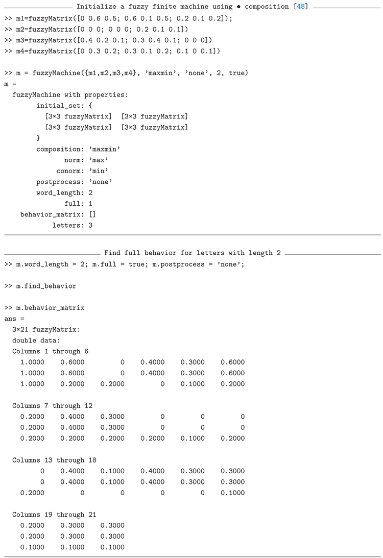
The fuzzyMachine module implements operations for finding behavior, reduction and minimization of FFMach. A FFMach is defined by a set of fuzzy matrices, one for each input/output pair of words. These matrices are stored in a cell array and passed to the constructor. The user specifies the composition type, the maximum word length to consider, and whether to return the full behavior matrix, a reduced or a minimized one.
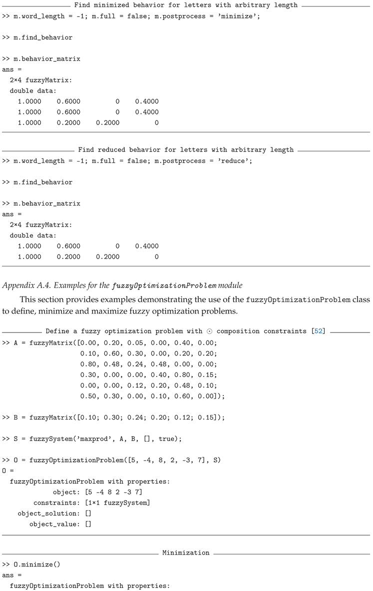
The main method find_behavior() applies the matrices to compute the machine’s behavior. If postprocessing is enabled, the resulting behavior matrix is reduced or minimized by eliminating redundant columns or states. The minimization procedure removes states whose behavior vectors can be expressed as fuzzy linear combinations of others.
All compositions listed in Section 6.1 are supported. The final behavior matrix is stored internally and can be accessed or exported for further analysis.
Examples are provided in Appendix A.3.
6.5. The fuzzyOptimizationProblem Module
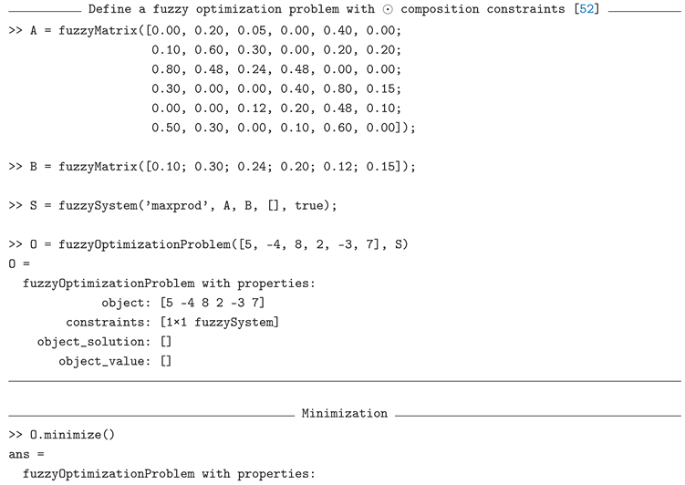
The fuzzyOptimizationProblem class provides a unified interface for solving fuzzy linear optimization problems of the form described in Section 4.5. A problem instance is created by specifying:
- an objective weight (cost) vector C;
- a system of constraints defined by a fuzzySystem object and supporting all of the fuzzySystem options such as compositions, and inequalities
Internally, the functions first solve the inverse problem for the fuzzySystem object to obtain the complete solutions set for the system of constraints. Then, it either evaluates the objective function on all solutions, according on the optimization goal.
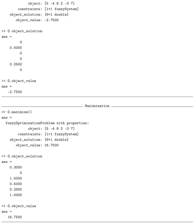
The methods minimize() and maximize() fill the object_solution and the object_value properties of the fuzzyOptimizationProblem object containing respectively, the optimal fuzzy vector x and the objective value z for the optimization problem. All properties of the system of constrains are held in the fuzzySystem object (e.g., consistency status or complete solutions set).
Examples of usage are provided in Appendix A.4.
7. Conclusions
In 1977 Peeva finished her PhD Thesis on categories of stochastic machines. The main attention was paid on computing behavior, establishing equivalence of states and equivalence of stochastic machines, as well as on reduction and minimization. All these problems were solved for stochastic machines, using linear algebra: they require solving linear system of equations with traditional algebraic operations, establishing linear dependence or linear independence of vectors, Noetherian property. After 1980 she was interested in similar problems, but for finite fuzzy machines. Nevertheless that stochastic machine seems to be similar to fuzzy machine, the main obstacle was that linear algebra and fuzzy algebras are completely unrelated. In order to investigate fuzzy machines, two types of algebras, called algebra and product algebra have been developed. The role played by these algebras in the theory of and product FFMachs is supposed to be the same as that played by linear algebra in the theory of stochastic machines. But these algebras propose tremendous manipulations for solving problems for FFMachs. Supplementary, there are several issues in [56], that are either incomplete or confused. This motivated the author to develop theory, algorithms and software for FFMachs. Obviously developing theory and software for solving problems for FFMachs requires first to develop theory and software for FRC and then to implement it for FFMachs. At this time these problems were open and she intended first to develop method, algorithm and software for solving FLSEs when the composition is , then to implement it to FFMachs. In 1980 she had no idea whether the solution exists and how long it will take her to solve the problems. Just now, after 40 years, we have positive answers to all these questions.
She worked on this subject with great pleasure during the years with her bachelor, master and PhD students, now Prof. Dr. Yordan Kyosev, Assoc. Prof. Dr. Zlatko Zahariev, Dobromir Petrov and Ivailo Atanassov to whom she would like to express deep and heartfelt gratitude.
Zlatko Zahariev joined this work in 2005 as a PhD student under the supervision of Prof. DSc. Ketty Peeva. His main focus was on developing algorithmic versions the methods, creating their software implementation, and contributing to the ongoing effort toward designing unified algorithms for solving the problems described in this paper. He considers himself fortunate to have the opportunity to work under Prof. DSc. Peeva’s guidance, and is deeply grateful to her for the years of meaningful and fulfilling scientific collaboration.
The authors thank the journal team for the special offer to write this article.
Author Contributions
Conceptualization, K.P. and Z.Z.; methodology, K.P. and Z.Z.; software, Z.Z.; validation, K.P. and Z.Z.; formal analysis, K.P. and Z.Z.; investigation, K.P.; resources, K.P.; data curation, K.P. and Z.Z.; writing—original draft preparation, K.P. and Z.Z.; writing—review and editing, K.P. and Z.Z.; visualization, K.P. and Z.Z.; supervision, K.P. All authors have read and agreed to the published version of the manuscript.
Funding
This research received no external funding
Abbreviations
The following abbreviations are used in this manuscript:
| FRC | fuzzy relational calculus |
| FFM | finite fuzzy matrix |
| FRE | fuzzy relation equation |
| FLSEs | fuzzy linear system of equations |
| FLSIs | fuzzy linear system of inequalities |
| FFMach | Finite fuzzy machine |
Appendix A. Examples
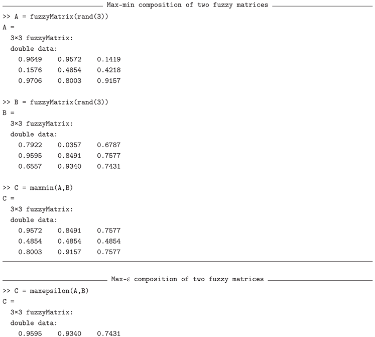
Appendix A.1. Examples for the fuzzyMatrix module
This section provides usage examples for the fuzzyMatrix module, including initialization, basic operations, and several types of fuzzy matrix composition.
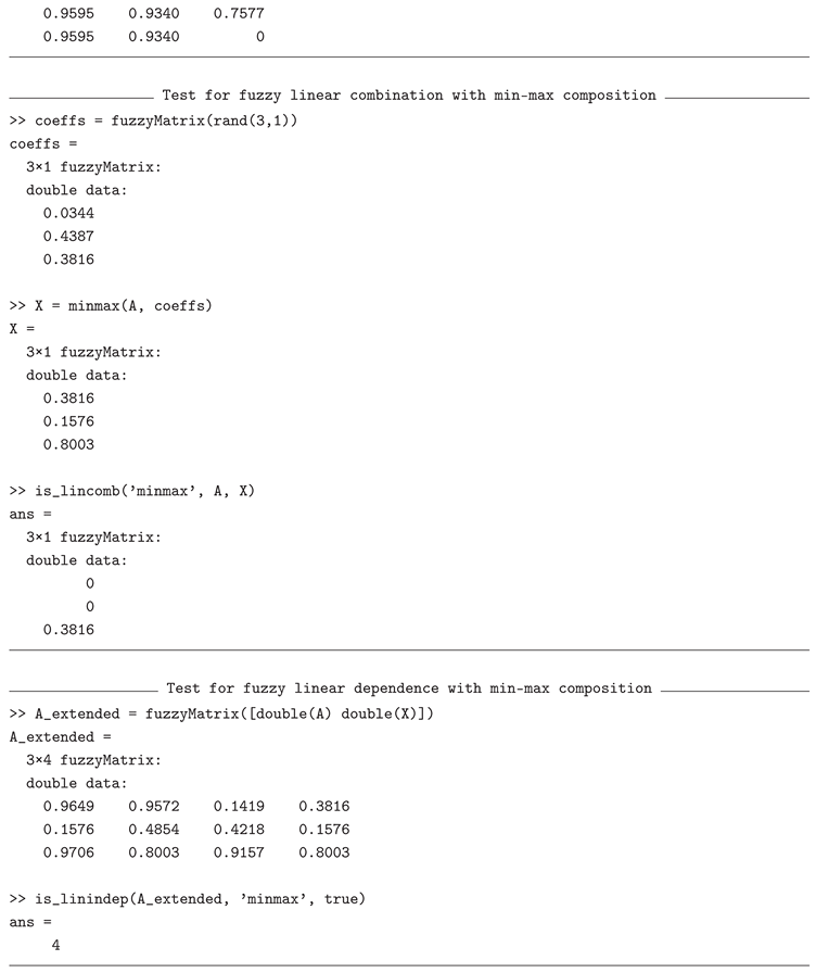
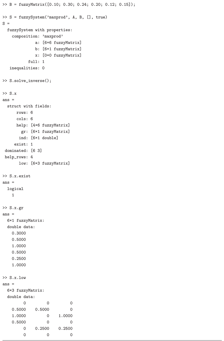
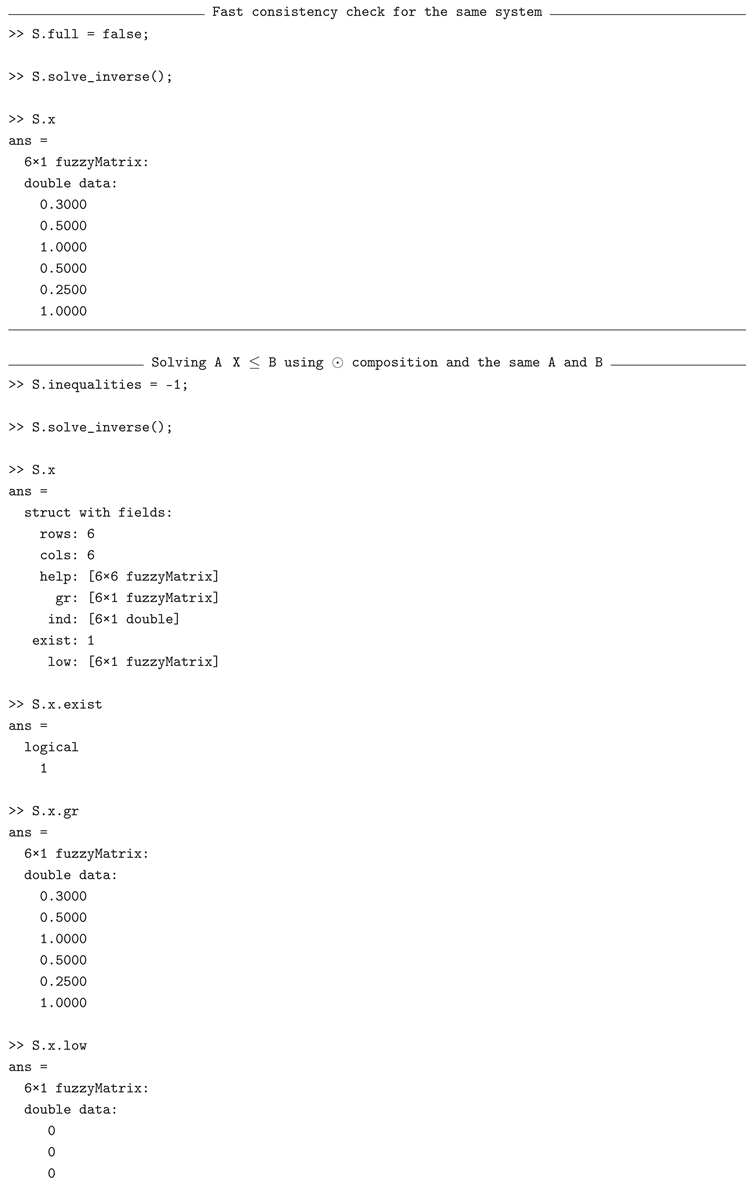
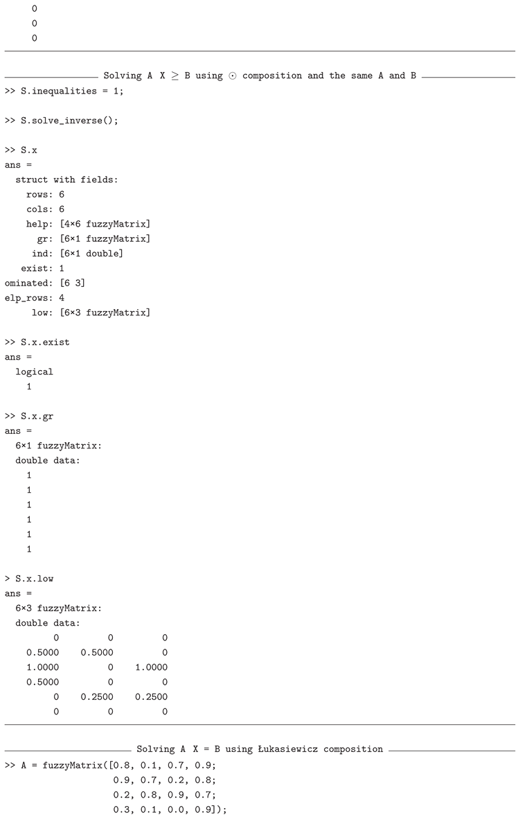
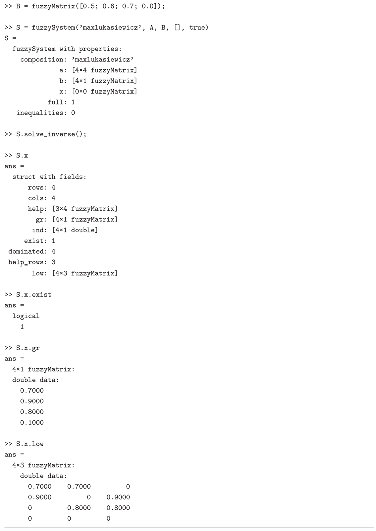
Appendix A.2. Examples for the fuzzySystem module
This section provides example uses of the fuzzySystem class, illustrating how to construct and solve fuzzy relational systems under various compositions and inequality types.
Appendix A.3. Examples for the fuzzyMachine module
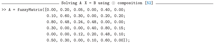
Appendix A.4. Examples for the fuzzyOptimizationProblem module
This section provides examples demonstrating the use of the fuzzyOptimizationProblem class to define, minimize and maximize fuzzy optimization problems.
References
- MacLane, S.; Birkhoff, G. Algebra. Macmillan, New York, 1979.
- Sanchez, E. Equations de Relations Floves. Thèse Biologie Humaine, 1972, Marseile, France.
- Sanchez, E. Solution in Composite Fuzzy Relation Equations: Application to Medical Diagnosis in Brouwerian Logic. Fuzzy Automata and Decision Processes 1977, Elsevier North-Holland, INC pp. 221-234,. [CrossRef]
- Sanchez, E. Resolution of composite fuzzy relation equations. Information and Control 1976, vol. 30, pp. 38–48.
- Higashi, M.; Klir, G.J. Resolution of finite fuzzy relation equations. FSS 1984, vol. 13 (1), pp. 65–82. [CrossRef]
- Czogała, E.; Drewniak, J.; Pedricz, W. Fuzzy relation equations on a finite set. FSS 1982, vol. 7(1), pp. 89-101. [CrossRef]
- Miyakoshi, M.; Shimbo, M. Lower solutions of systems of fuzzy equations. FSS 1986, vol. 19 pp. 37–46.
- Pappis, C.P.; Sugeno, M. Fuzzy relational equations and the inverse problem. FSS 1985, vol. 15, pp. 79–90. [CrossRef]
- Adomopoulos, G.; Pappis, C. Some results on the resolution of fuzzy relation equations. FSS 1993, vol.60 (1), pp. 83–88. [CrossRef]
- Pappis, C.; Adamopoulos, G. A software routine to solve the generalized inverse problem of fuzzy systems. FSS 1992, vol. 47, pp. 319-322. [CrossRef]
- Pappis, C.; Adamopoulos, G. A computer algorithm for the solution of the inverse problem of fuzzy systems. FSS 1991, vol. 39, pp. 279–290. [CrossRef]
- Peeva, K. Fuzzy linear systems. FSS 1992, vol. 49, pp.339–355.
- Chen, L.; Wang, P. Fuzzy relational equations (I): The General and Specialized Solving Algorithms. Soft Computing 2002, vol. 6, pp. 428–435. [CrossRef]
- Peeva, K. Universal algorithm for solving fuzzy relational equations. Italian Journal of Pure and Applied Mathematics 2006, vol. 19, pp. 9–20.
- Peeva, K.; Kyosev, Y. Fuzzy relational calculus – theory, applications and software (with CD-ROM), Advances in Fuzzy Systems – Applications and Theory, vol. 22, World Scientific Publishing Company, 2004.
- Bourke, M.M.; Fisher, D.G. Solution algorithms for fuzzy relational equations with max–product composition. FSS 1998, vol. 94, pp. 61–69. [CrossRef]
- Di Nola, A.; Pedrycz, W.; Sessa, S.; Sanchez, E. Fuzzy Relation Equations and Their Application to Knowledge Engineering. Kluwer Academic Press, Dordrecht/Boston/London, 1989. [CrossRef]
- Loetamonphong, J.; Fang, S.-C. An efficient solution procedure for fuzzy relational equations with max–product composition. IEEE Transactions on Fuzzy Systems 1999, vol. 7 (4), pp.441–445. [CrossRef]
- Markovskii, A.V. On the relation between equations with max–product composition and the covering problem. FSS, 2005, vol. 153 (2), pp. 261-273. [CrossRef]
- Bartl, E.; Belohlávek, R. Sup-t-norm and inf-residuum are a single type of relational equations. Int. J. Gen. Syst. 2011, vol. 40(6) pp. 599-609. [CrossRef]
- Feng Sun. Conditions for the existence of the least solution and minimal solutions to fuzzy relation equations over complete Brouwerian lattices. Information Sciences, 2012, vol. 205, pp. 86-92. [CrossRef]
- Nosková, L.; Perfilieva, I. System of fuzzy relation equations with sup-* composition in semi-linear spaces: minimal solutions. 2007 IEEE International Fuzzy Systems Conference, London, UK, 2007, pp. 1-6. [CrossRef]
- Perfilieva, I.; Nosková, L. System of fuzzy relation equations with inf-→ composition: Complete set of solutions. FSS 2008, vol 159 (17), pp. 2256-227. [CrossRef]
- Bartl, E. Minimal solutions of generalized fuzzy relational equations: Probabilistic algorithm based on greedy approach. FSS 2015, vol. 260, pp. 25-42. [CrossRef]
- Bartl, E.; Klir, G. J. Fuzzy relational equations in general framework. Int. J. Gen. Syst. 2014, vol. 43(1), pp. 1-18. [CrossRef]
- Medina, J.; Turunen, E.; Bartl, E. ; Juan Carlos Díaz-Moreno. Minimal Solutions of Fuzzy Relation Equations with General Operators on the Unit Interval. IPMU 2014 (3), pp. 81-90. [CrossRef]
- De Baets, B. Analytical solution methods for fuzzy relational equations. In: Fundamentals of Fuzzy Sets, The Handbooks of Fuzzy Sets Series, vol. 1, D. Dubois, H. Prade (Eds.), Kluwer Academic Publishers 2000, pp. 291–340. [CrossRef]
- Li, P.; Fang, S.-C. A survey on fuzzy relational equations. Part I: Classification and solvability. Fuzzy Optimization and Decision Making 2009, vol. 8, pp. 179–229. [CrossRef]
- Molai, A.A.; Khorram, E. An algorithm for solving fuzzy relation equations with max-T composition operator. Information Sciences 2008, vol. 178(5), pp.1293-1308. [CrossRef]
- Shieh, B.-S. New resolution of finite fuzzy relation equations with max-min composition. International Journal of Uncertainty Fuzziness Knowledge Based Systems 2008, vol 16 (1), pp. 19–33. [CrossRef]
- Shivanian, E. An algorithm for finding solutions of fuzzy relation equations with max-Lukasiewicz composition, Mathware & Soft Computing, 2010 vol. 17, pp. 15-26.
- Wu, Y.-K.; Guu, S.-M. An efficient procedure for solving a fuzzy relational equation with max-Archimedean t-norm composition. IEEE Transactions on Fuzzy Systems 2008, vol. 16 (1), pp. 73–84. [CrossRef]
- Bartl, E.; Belohlávek, R. Hardness of Solving Relational Equations. IEEE Trans. Fuzzy Syst. 2015, vol. 23(6), pp. 2435-2438. [CrossRef]
- http://www.mathworks.com/matlabcentral/fleexchange/6214-fuzzy-relational-calculus-toolbox-rel-1-01.
- Bartl, E.; Trnecka, M. Covering of minimal solutions to fuzzy relational equations. International Journal of General Systems 2021, vol. 50 (2), pp. 117–138. [CrossRef]
- Lin, J.-L. On the relation between fuzzy max-Archimedean t-norm relational equations and the covering problem. FSS 2009, vol. 160 (16), pp. 2328–2344. [CrossRef]
- Lin, J.-L.; Wu, Y.-K.; Guu, S.-M. On fuzzy relational equations and the covering problem. Information Sciences, 2011, Vol. 181, (14), pp 2951-2963. [CrossRef]
- http://www.mathworks.com/matlabcentral, fuzzy-calculus-core-fc2ore (2010).
- Grätzer, G. General Lattice Theory, Akademie-Verlag, Berlin, 1978.
- H<i>a</i>`jek, P. Metamathematics of Fuzzy Logic, Kluer, Dordecht, 1998.
- Peeva, K. Resolution of Fuzzy Relational Equations – Method, Algorithm and Software with Applications. Inf. Sci. 2013, vol 234, pp. 44 - 63. [CrossRef]
- K. Peeva, G. K. Peeva, G. Zaharieva, Zl. Zahariev, Resolution of max–t-norm fuzzy linear system of equations in BL-algebras, AIP Conference Proceedings, Vol. 1789, 060005, 2016. [CrossRef]
- Zl. Zahariev, G. Zl. Zahariev, G. Zaharieva, K. Peeva, Fuzzy relational equations – Min-Goguen implication, AIP Conference Proceedings, Vol. 2505, 120004, 2022. [CrossRef]
- Zl. Zahariev, Fuzzy Relational Equations And Inequalities – Min-Łukasiewicz Implication, AIP Conference Proceedings, Vol. 2939, 030011, 2023. [CrossRef]
- Santos, E. S. Maximin automata Information and Control, 1968, vol. 13 pp. 363-377.
- Santos,E. S. Maximin, minimax and composite sequential mashines.J. Math. Anal. Appl., 1968, vol. 24, pp. 246-259. [CrossRef]
- Santos E., S.; Wee, W. G. General formulation of sequential machines. Information and Control, 1968, vol. 12 (1), pp. 5-10.
- Peeva, K; Zahariev, Zl. Computing behavior of finite fuzzy machines – Algorithm and its application to reduction and minimization. Information Sciences, 2008, vol. 178, pp. 4152-4165. [CrossRef]
- Fang, S.-. G; Li G. Solving Fuzzy Relation Equations with Linear Objective Function. FSS, 1999 , vol. 103, pp. 107–113. [CrossRef]
- Guu, S. M; Wu Y-K. Minimizing a linear objective function with fuzzy relation equation constraints. Fuzzy Optimization and Decision Making, 2002, vol. 4 (1), pp.347-360. [CrossRef]
- Loetamonphong, J.; Fang, S.-C. (2001) Optimization of fuzzy relation equations with max-product composition. FSS, 2001, vol. 118 (3), pp. 509–517. [CrossRef]
- Peeva, K.; Zahariev, Zl.; Atanasov, I. Optimization of linear objective function under max-product fuzzy relational constraints. In Proceedings of the 9th WSEAS International Conference on FUZZY SYSTEMS (FS’08) – Advantest Topics on Fuzzy Systems, Book series: Artificial Intelligence Series – WSEAS Sofia, Bulgaria, May 2-4, , ISBN: 978-960-6766-56-5. 2008. [Google Scholar]
- Peeva, K.; Petrov, D. Optimization of Linear Objective Function under Fuzzy Equation Constraint in BL–Algebras – Theory, Algorithm and Software. In: Intelligent Systems: From Theory to Practice. Studies in Computational Intelligence, Sgurev, V., Hadjiski, M., Kacprzyk, J. (eds), 2010 vol 299. Springer, Berlin, Heidelberg.
- Wang P.Z.; Zhang D.Z.; Sanchez E.; Lee E.S. Latticized linear programming and fuzzy relation inequalities. Math. Anal. Appl., 1991, vol. 159 (1), pp. 72-87. [CrossRef]
- Wu, Y-K; Guu S. M.; Liu Y.-C. An Accelerated Approach for Solving Fuzzy Relation Equations with a Linear Objective Function. |textitIEEE Transactions on Fuzzy Systems, 2002, vol. 10(4), pp. 552–558. [CrossRef]
- Santos, E. S. On reduction of maxi-min machines. J. Math. Anal. Appl., 1972 vol. 40 pp. 60-78.
Figure 2.
Architecture of the Fuzzy Calculus Core software.
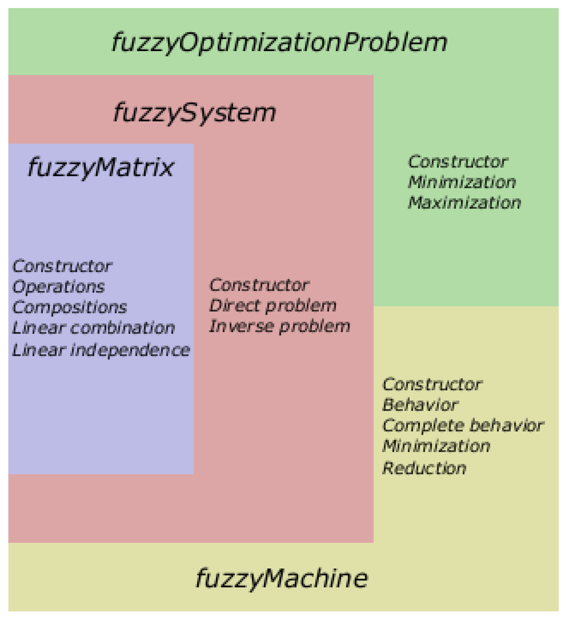

Table 1.
t-norms and s-norms.
| t-norm | name | expression | s-norm | name | expression | |
|---|---|---|---|---|---|---|
| minimum, Gödel t-norm | maximum, Gödel t-conorm | |||||
| Algebraic product |
Probabilistic sum | |||||
| ukasiewicz t-norm | Bounded sum |
Table 2.
– initial fragment.
| … | … | ||||
|---|---|---|---|---|---|
| … | … | ||||
| … | … | ||||
| … | … | … | … | … | … |
| … | … | ||||
| length l | … | … |
Disclaimer/Publisher’s Note: The statements, opinions and data contained in all publications are solely those of the individual author(s) and contributor(s) and not of MDPI and/or the editor(s). MDPI and/or the editor(s) disclaim responsibility for any injury to people or property resulting from any ideas, methods, instructions or products referred to in the content. |
© 2025 by the authors. Licensee MDPI, Basel, Switzerland. This article is an open access article distributed under the terms and conditions of the Creative Commons Attribution (CC BY) license (http://creativecommons.org/licenses/by/4.0/).
Copyright: This open access article is published under a Creative Commons CC BY 4.0 license, which permit the free download, distribution, and reuse, provided that the author and preprint are cited in any reuse.


