Chaotic Interaction Between Thermodynamic Systems

1. Introduction

In the previous study [1], our main aim was to prove that the interaction in the dark side is chaotic. In Ref. [1] we consider dark matter and dark energy as open -the grand canonical- thermodynamic system. We introduce a new interaction schema and show that the interaction between dark matter and dark energy under conditions $\delta Q\ne 0$, $\delta N\ne 0$ and $dV=0$ is chaotic. We also predicted that obtained results could be generalized to all particle and thermodynamic systems. Therefore, we proposed a new physics law based on these results:

–

“The dynamics of all coupled interacting particle and thermodynamic systems are chaotic.”

In addition, we introduced a new definition of chaos for the first time in the literature:

–

“Chaos is the minimum action of the coupled, synchronized or self-organized interacting systems.”

In this study, we will try to extend the discussion to different thermodynamic systems and also to give the physical and philosophical background to deepen the new physics law and chaos definition mentioned here. For this reason, we will study the dynamics of two thermodynamic systems interacting under different conditions to support the previous results. Thus, we will consider two different situations for the interacting thermodynamic systems: i) $\delta Q\ne 0$, $\delta N=0$ and $dV=0$ and ii) $\delta Q\ne 0$, $\delta N\ne 0$ and $dV\ne 0$. Using the same interaction schema in [1], we will discuss chaotic dynamics for these cases. Additionally, we will briefly discuss the “minimum action of nature” and “complexity”.

This work is organized as follows: In Section 2, we briefly introduce the interaction model based on Ref. [1]. In Section 3, we consider a case for $\delta Q\ne 0$, $\delta N=0$, and $dV=0$. In Section 4, we consider a case for $\delta Q\ne 0$, $\delta N\ne 0$, and $dV\ne 0$. In both sections, we introduce new interaction equations for two cases, and we will analyze the phase space and chaotic behaviours of the interacting systems. In Section 5, we will discuss the new results obtained and the physical and philosophical aspects of the proposed laws and definitions. In addition, in this section, we will also introduce a new action principle and definition of the complexity. Finally, in the last Section 6, conclusions are presented.

2. The Model

The energy exchange for any open thermodynamic systems is given by

$$\begin{array}{c}\hfill dU=\delta Q+\sum _{i=1}^N\delta W_i\end{array}$$

(1)

where $dU$ corresponds to energy exchange in the system, $\delta Q$ is heat changes, and $\delta W_i$ denotes work which is done ont he system. The energy exchanges for two coupled interacting systems can be given in the form [1]:

$$\begin{array}{c}\hfill d{U}_1\left(x_2\right)=\delta Q_1\left(x_1\right)+\delta W_1\left(x_1\right)+\delta N_1\left(x_1\right)\end{array}$$

(2a)

$$\begin{array}{c}\hfill d{U}_2\left(x_1\right)=\delta Q_2\left(x_2\right)+\delta W_2\left(x_2\right)+\delta N_2(x_{2)}\end{array}$$

(2b)

where $d{U}_1\left(x_2\right)$ and $d{U}_2\left(x_1\right)$ denote the energy exchanges on the system 1 and 2, respectively.

Here, $x_1$ is considered the energy flux passing through system 1, and $x_2$ is considered the energy flux passing through system 2. In energy exchanges between systems, the total energy will be conserved:

$$\begin{array}{c}\hfill \oint dU(x_i)=0\end{array}$$

(3)

where $i=1,2$. At the same time, total energy is conservative:

$$\begin{array}{c}\hfill \sum _{i=1}{E}_i=const\end{array}$$

(4)

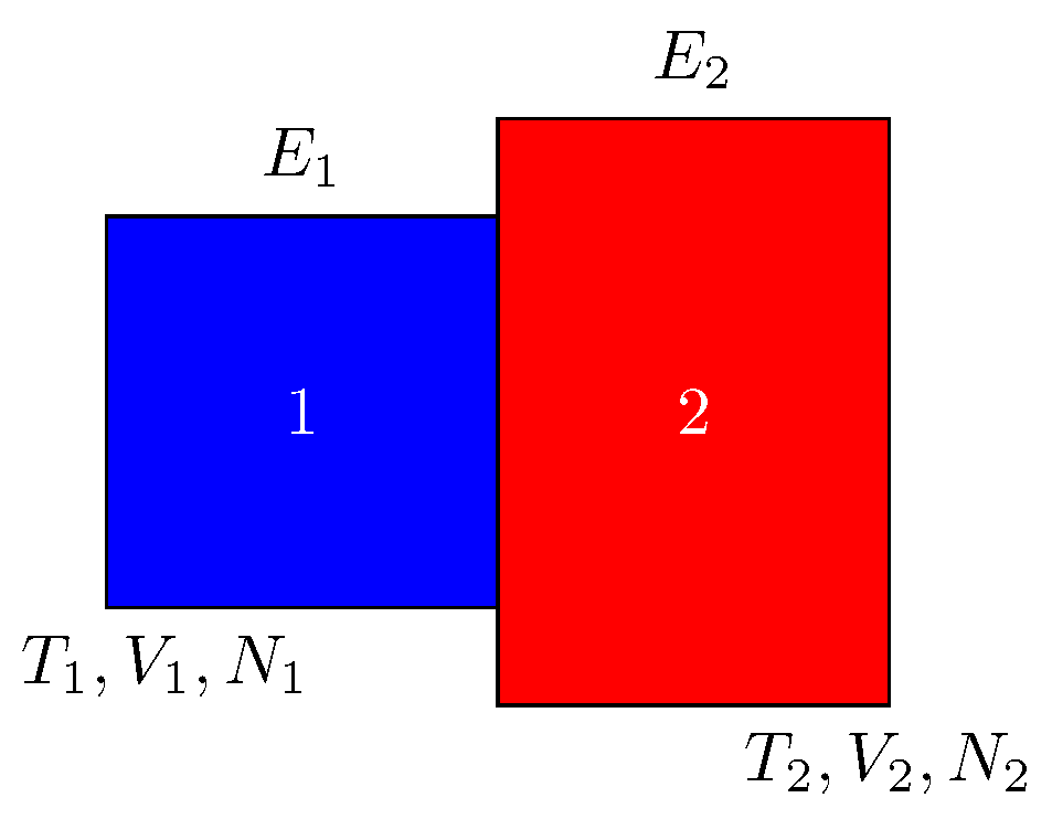
Let us imagine that two separate thermodynamic systems with different energies, temperatures, volumes, and numbers of particles are in contact with each other, as in Figure 1. According to the traditional thermodynamic approach, if these two systems are not in equilibrium, that is, for example, $T_1\ne T_2$, $p_1\ne p_2$, or ${\mu }_1\ne {\mu }_2$, then the systems are far from equilibrium and will continue to interact with each other until they reach equilibrium. Changes in internal energy in both systems can be derived from Eqs.(2) and (3).

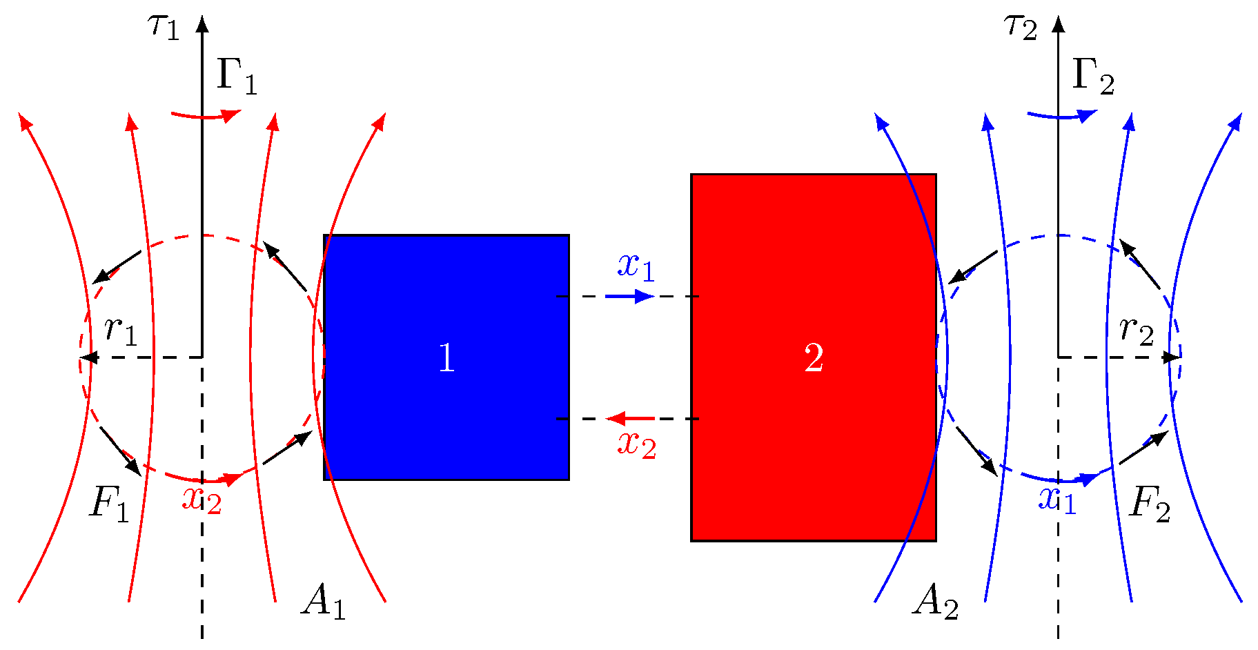
In this study, two models are $\delta Q\ne 0$, $\delta N=0$, $dV=0$ and $\delta Q\ne 0$, $\delta N\ne 0$, $dV\ne 0$. We will consider a different situation. Since the interactions in the self-interaction loops will remain the same for both cases, we will focus only on the mutual interaction in the next section. As is well known, the mutual and self-interaction scheme is as follows:

Self-interactions of two coupled thermodynamic systems given in Ref. [1] are

$${\displaystyle \frac{d{\Gamma }_1}{dt}}=1-x_1{x}_2,{\displaystyle \frac{d{\Gamma }_2}{dt}}=1-x_1{x}_2$$

(5)

For solid systems that are assumed not to rotate while in contact, Eq.(5) can be written as

$$\begin{array}{c}\hfill {\displaystyle \frac{d{\Gamma }_1}{dt}}=-x_1{x}_2,{\displaystyle \frac{d{\Gamma }_2}{dt}}=-x_1{x}_2.\end{array}$$

(6)

Self-interaction loops are not defined in standard statistical thermodynamics. Therefore, the interaction picture still needs to be completed. Mutual interactions do not formally connect the interacting systems. However, systems behave with each other as sources. We show in the previous study [1] that self-interaction loops connect resources in the interaction schema. Therefore, self-interact loops have new hidden variables and vectorial fields, unlike the classical interaction schema. It is clear that both the new interaction schema and new concepts strongly indicate the presence of the new thermodynamic laws.

The self-interaction loops represent the hidden attractors. Looking at the literature, it can be seen that the idea of hidden attractor is not new and appears in dynamic systems. The concept of hidden attractors was first introduced in connection with Hilbert’s 16th problem formulated in 1900 [2]. Kuznetsov et al. reported the chaotic hidden attractor in Chua’s circuit [3,4,5]. This research has since led to further efforts to locate hidden attractors in various examples [6,7,8,9,10,11].

3. Case I: $\mathit{\delta }\mathit{Q}\ne \mathbf{0}$, $\mathit{\delta }\mathit{N}=\mathbf{0}$ and $\mathit{dV}=\mathbf{0}$

For the case $\delta Q\ne 0$, $\delta N=0$ and $dV=0$ the mutual interaction equation as

$${\displaystyle \frac{d{x}_1}{dt}}={\Gamma }_1{x}_2,{\displaystyle \frac{d{x}_2}{dt}}={\Gamma }_2{x}_1$$

(7)

where ${\Gamma }_{1,2}$ are the non-holonomic variables which are denote energy transfer velocity.

By using Eqs.(5) and (7) we obtain interaction equation for the coupled and interacting two canonical ensembles i.e., thermodynamic systems as

$$\begin{array}{ccc}\hfill {\displaystyle \frac{d{x}_1}{dt}}& =& x_2{x}_3\hfill \\ \hfill {\displaystyle \frac{d{x}_2}{dt}}& =& (x_3-q)x_1\hfill \\ \hfill {\displaystyle \frac{d{x}_3}{dt}}& =& 1-x_1{x}_2\hfill \end{array}$$

(8)

where q is the control parameters $q={\Gamma }_1-{\Gamma }_2$. Eq.(8) is a non-linear and which describes the dynamics of the interacting systems via only heat transfer.

Using the Runga-Kutta method and the linearized algorithm [12], we numerically solved Eq.(8) with FORTRAN 90. We obtained phase-space solutions and Lyapunov exponents belonging to the coupling equations. Phase trajectories and Lyapunov exponents are given in Figure 3, Figure 4 and Figure 5 and Figure 6, respectively.

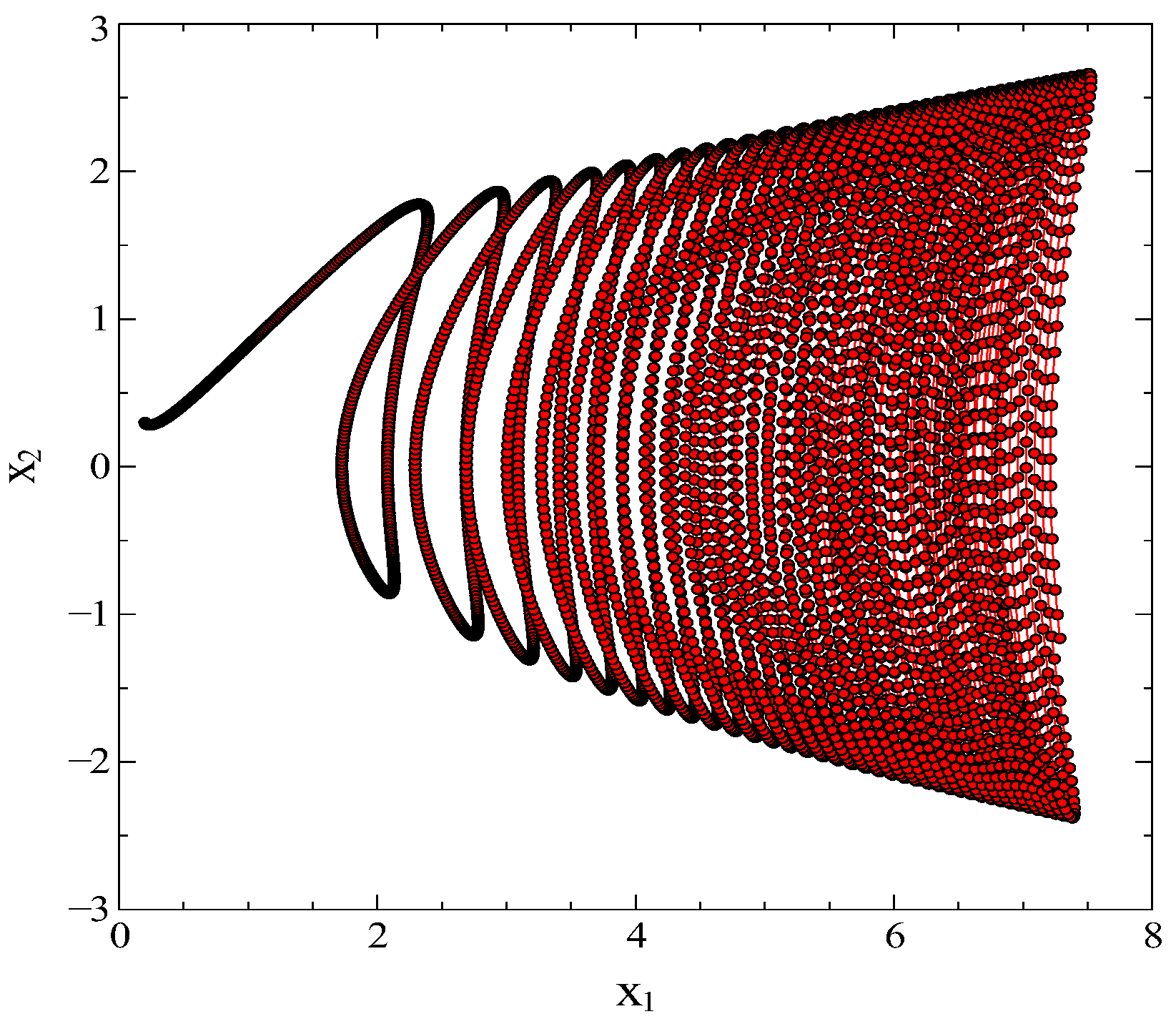
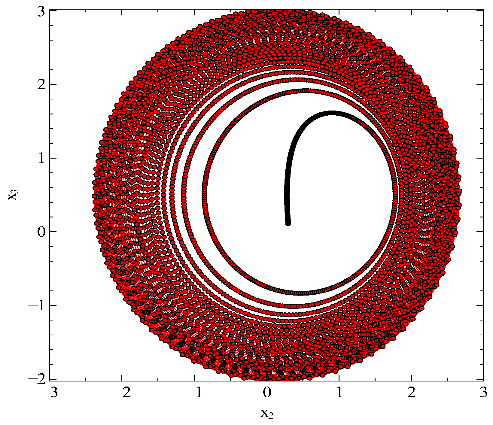
The solutions of $x_1$ and $x_2$ for the control parameters $q=3.46$ are given in Figure 3. It is clearly seen that the trajectory in the $x_1-x_2$ plane does not intersect and repeat in the attractor basin. One can see that the attractor appears around $x_2=0$ and the trajectory proceeds in the $x_1$ direction.

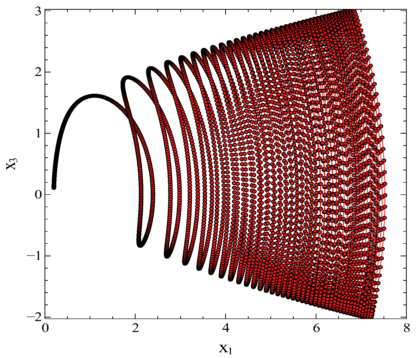
Similarly, solutions of $x_1$ and $x_3$ for the control parameters $q=3.46$ are given in Figure 4, the attractor appears in the $x_1-x_3$ plane around $x_3=0$. One can see that orbit does not make periodic changes and moves in the $x_1$ direction without cutting itself. In fact, the attractor behaviours in Figure 3 and Figure 4 can be clearly seen in Figure 5. In fact, the attractor and the trajectory appear around $x_2=0$ and $x_3$ on $x_2-x_3$ in Figure 5.

Additionally, we have tested that the character of the phase-space solution does not change for the various running step time. The chaotic attractor is located at only one fixed point.

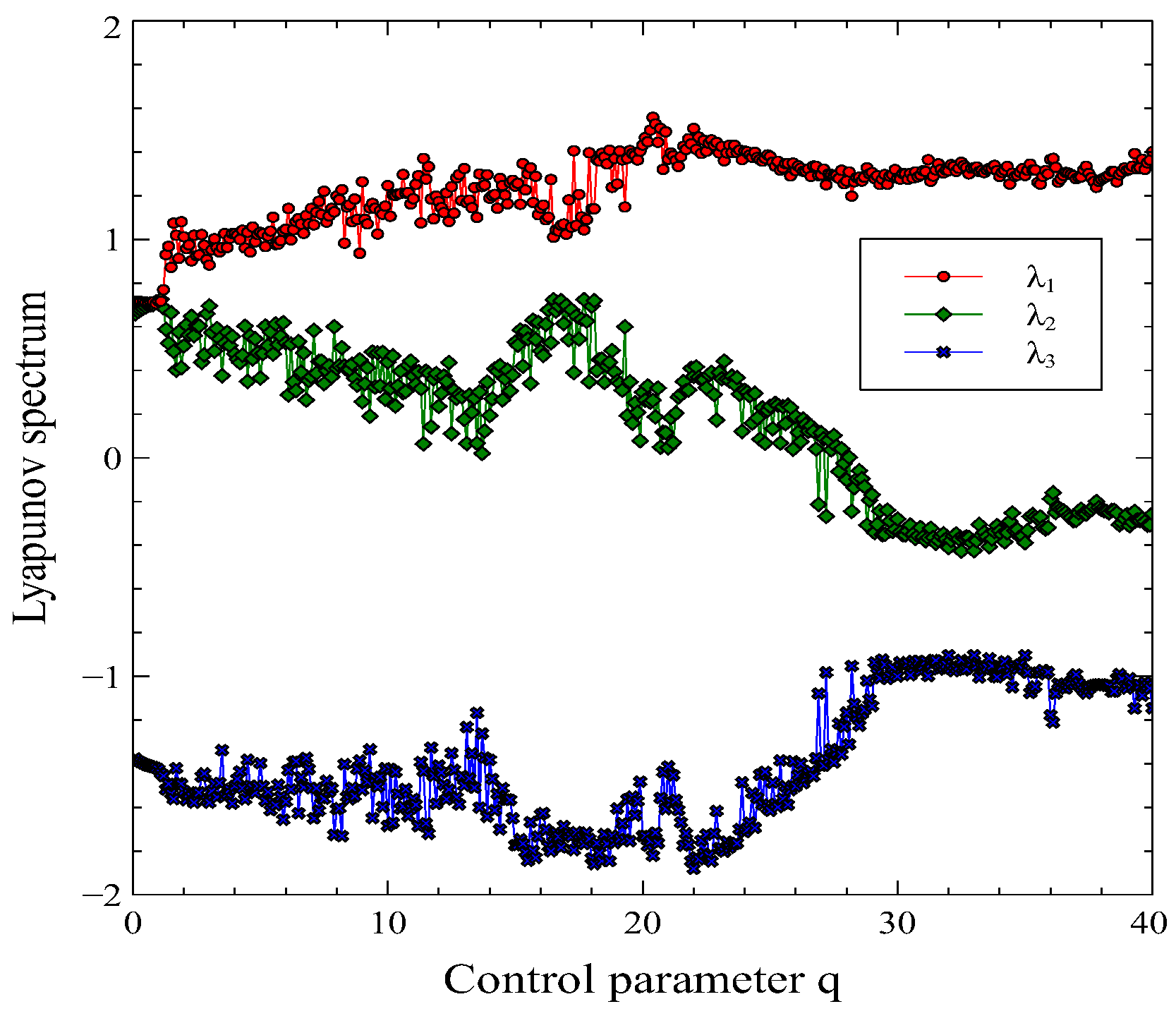
Now we discuss the Lyapunov [13] spectrum of the system in Eq.(8). Positive Lyapunov exponents are known to indicate chaotic behaviour of the system. We obtained the Lyapunov spectrum using the Wolf algorithm and plotted it in Figure 6. One can see that the system produces three positive Lyapunov exponents in this interaction schema. As seen in Figure 6, one of the exponents which receive a red curve is always positive for all values q. However, the other two Lyapunov exponents (yellow and blue curves) take negative and positive values for the different q values. It is strongly provided that the dynamics of the two coupled and interacting canonical or close thermodynamic systems are chaotic like two grand canonical systems [1].

4. Case II: $\mathit{\delta }\mathit{Q}\ne \mathbf{0}$, $\mathit{\delta }\mathit{N}\ne \mathbf{0}$ and $\mathit{dV}\ne \mathbf{0}$

In this section, we will also consider volume changes. As a result of the interaction, the volume of the systems may change, and this prevents work on the system. The work performed on the system is defined as $\delta W=-pdV$. In this case, the equations Eq.(8) can be written in the following form:

$$\begin{array}{ccc}\hfill {\displaystyle \frac{d{x}_1}{dt}}& =& x_2{x}_3-x_1-{\int }_0^{\tau }{x}_1\left(t\right)dt\hfill \\ \hfill {\displaystyle \frac{d{x}_2}{dt}}& =& (x_3-q)x_1-x_2-{\int }_0^{\tau }{x}_2\left(t\right)dt\hfill \\ \hfill {\displaystyle \frac{d{x}_3}{dt}}& =& 1-x_1{x}_2\hfill \end{array}$$

(9)

The integral terms in the expression Eq.(9) represent the energy storage capacity in systems. Integral expressions do not contain non-linear terms. Therefore, contributions from these terms can be considered as constant contributions in the numerical solution. For simplicity, we define these integrals as ${\delta }_{1,2}$, where ${\delta }_1={\int }_0^{\tau }{x}_1\left(t\right)dt$ and ${\delta }_2={\int }_0^{\tau }{x}_2\left(t\right)dt$ we can simplify the solution. We can think of ${\delta }_{1,2}$ as control parameters that measure the energy storage capacity. In this case, rather than getting lost in the details of the numerical solution, it would be appropriate to include the behaviour of the system depending on the parameter ${\delta }_{1,2}$ for a fixed value q. Because, as can be seen in Figure 6, the system behaves chaotic for all q values. However, the chaotic dynamics in the system can be controlled depending on the energy storage capacity.

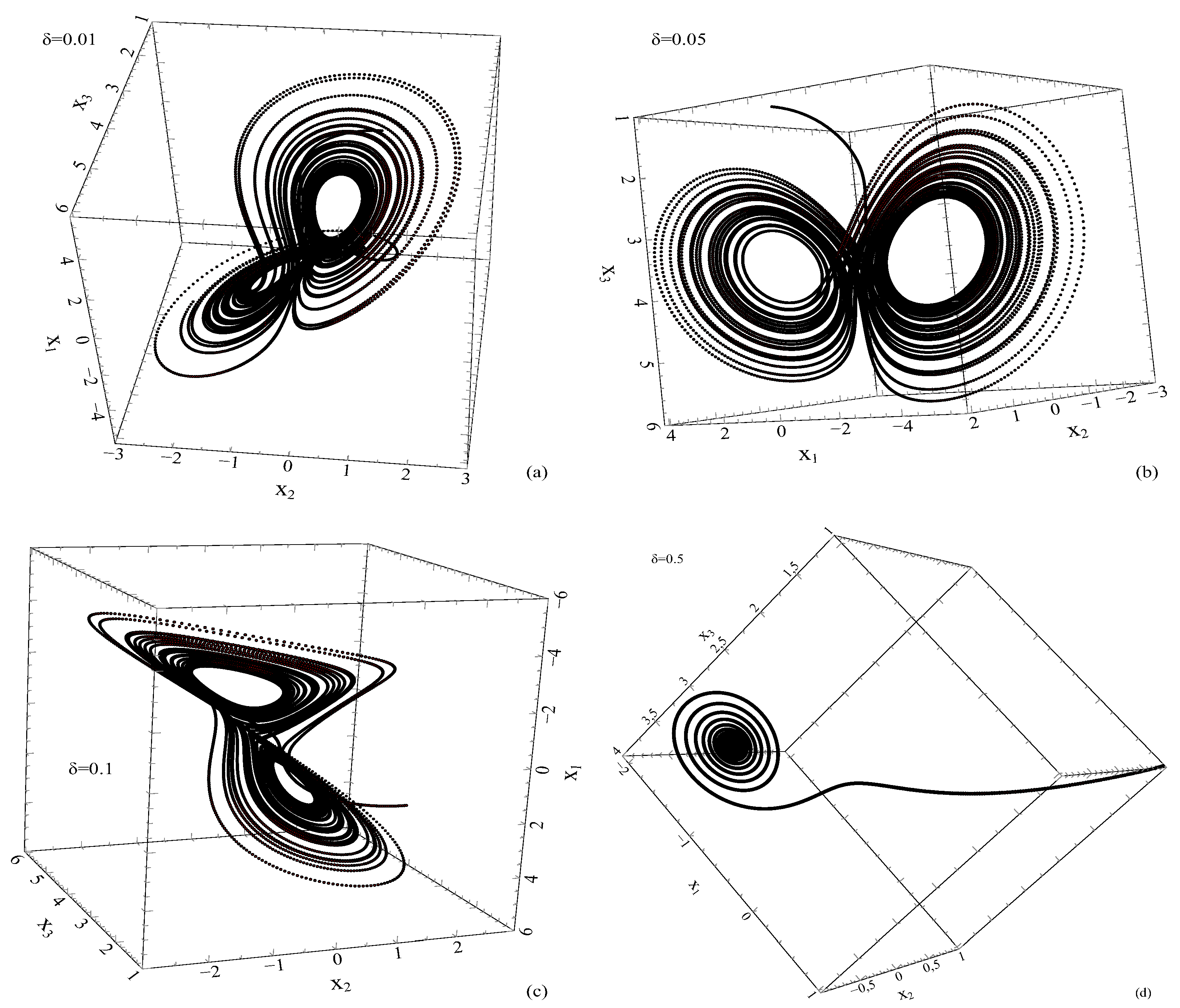
In order to maintain simplicity in the numerical solution, we will take $\delta ={\delta }_1={\delta }_2$ and solve Eq.(9) numerically for different values $\delta$. Using the Runga-Kutta method and the linearized algorithm $\delta$ values are given in Figure 7.

Figure 7 (a)-(d) for four different delta values $\delta =0.01$, $\delta =0.05$, $\delta =0.1$, and $\delta =0.5$ are plotted. As can be seen in Figure 7 (a)-(c), the existence of chaotic attractors in the phase space is observed for small values of $\delta$. But for $\delta =0.5$ the chaotic attractors disappear. We did not look for a critical value for $\delta$ here. However, we only wanted to show that for large values of the $\delta$ parameter, chaotic dynamics will disappear, and the system will go to a periodic or aperiodic solution. Here, $\delta$ acts as a control parameter.

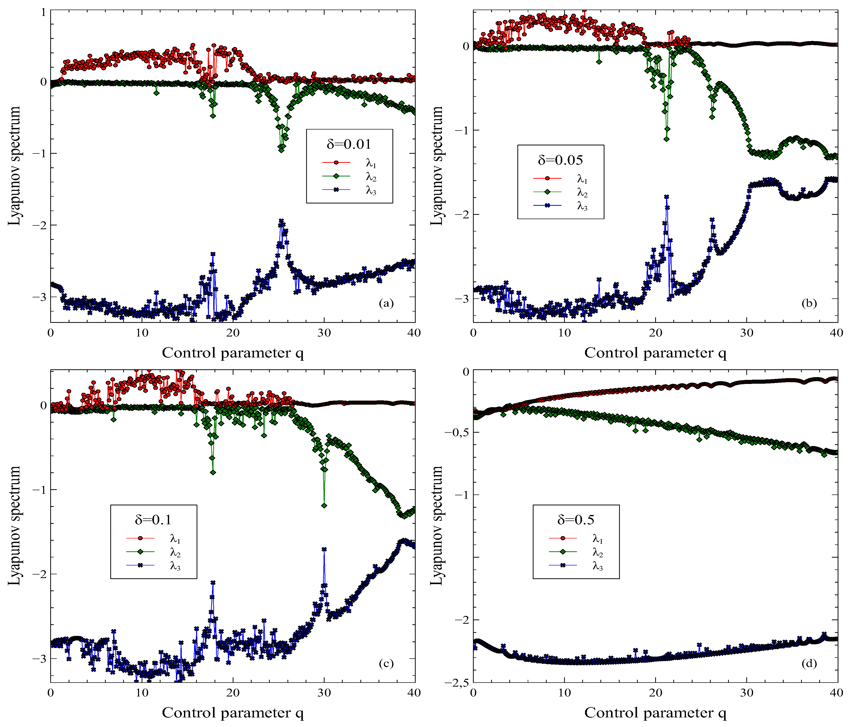
Similarly, we calculated the Lyapunov exponents for the same values $\delta$ and gave them in Figure 8. As can be seen in Figure 8 (a) and (c), there is at least one positive Lyapunov exponent in the spectrum for $\delta =0.01$, $\delta =0.05$ and $\delta =0.1$ For $\delta =0.5$, in Figure 8 (a), all exponents do not take negative values. As will be remembered, to say that the dynamics of the system are chaotic, there must be at least one positive exponent in the Lyapunov spectrum.

We would like to point out another important difference. For example, for conditions $\delta Q\ne 0$, $\delta N=0$ and $dV=0$, only one chaotic attractor appears in the phase space, while for case $\delta Q\ne 0$, $\delta N\ne 0$ it is seen that it is a chaotic attractor in the condition and $dV\ne 0$. The reason for this can be expressed as the system of equations given in Eq.(9) has a more complex structure.

Another important point is that $\delta ={\delta }_1={\delta }_2$ was chosen. Instead, if different values of ${\delta }_1$ and ${\delta }_2$ had been studied, two control parameters would have been included in the system. However, it is obvious that for small values ${\delta }_1$ and ${\delta }_2$, the system given by Eq.(9) will produce chaotic dynamics. Another point is that the expressions ${\delta }_1$ and ${\delta }_2$ could be written as a function of time. But it is clear that, in any case, the quantitative analysis will not change.

5. Discussion

In our previous work, we considered two thermodynamic systems interacting under the condition [1] $\delta Q\ne 0$, $\delta N\ne 0$, $dV=0$. We defined a new interaction scheme. We proved the validity of this interaction scheme by starting from the law of conservation of energy. From these results, we suggested that the energy interaction of dark matter and dark energy in particular should be chaotic.

In this current study, we have shown that the interaction dynamics of thermodynamic systems interacting under conditions $\delta Q\ne 0$, $\delta N=0$, $dV=0$ and $\delta Q\ne 0$, $\delta N\ne 0$, $dV\ne 0$ are chaotic. These new findings show that the proposed new law is universal for all interacting thermodynamic systems. However, although it is not based on a experimental and theoretical proof, it is possible to assume that the proposed law should also be valid for particle-particle interactions. We will return to this topic.

Now, we want to get back to the noteworthy problems: Why do we expect the dynamics of interacting systems to be chaotic? What could be the physical and philosophical equivalent of this question? These two questions are important. The answers to these questions are available in the proposed law and in the given definition. This law and definition clearly imply that: “Chaos minimizes the joint action”. To understand this, let us recall the trajectories in the Lorenz butterfly attractors. The Lorenz equation [14] is formed by writing three differential equations containing three first-order time derivatives in a coupled form. If these three equations were not coupled, that is, if they were in separable form, each equation would have separate solutions and separate trajectories. However, the coupled form of the equation produces a single common trajectory that minimizes all three variables simultaneously, which is the shortest possible path for the chosen parameters. It is not one of the shortest paths, but the only shortest path. This shows us that chaos produces the shortest path. This is why it leads to a correct conceptual description of this process. Once again, this definition implies the existence of a new law of physics, which is introduced here.

On the other hand, let us point out that there is no definition of chaos in the literature [15,16]. Chaos is generally called a process and is well known for its three basic features. These are; i) it arises from non-linear dynamics, ii) it shows sensitive dependence on the initial condition, and iii) its evolution over time is unpredictable [17,18,19,20,21,22,23,24,25,26,27,28,29,30,31]. Even so, one can find chaos definitions in the literature. For instance; the term chaos has first been used in 1975 by Li and York in their paper [32]: “Period three implies chaos”. Wiggins [24] define chaos as: “A dynamical system displaying sensitive dependence on initial conditions on a closed invariant set (which consists of more than one orbit) will be called chaotic”. Tabor [25]: “By a chaotic solution to a deterministic equation we mean a solution whose outcome is very sensitive to initial conditions (i.e., small changes in initial conditions lead to great differences in outcome) and whose evolution through phase space appears to be quite random.” Rasband [26]: “The very use of the word ’chaos’ implies some observation of a system, perhaps through measurement, and that these observations or measurements vary unpredictably. We often say observations are chaotic when there is no discernible regularity or order”. Prigogine defined chaos as ’order emerging from disorder’ in his book titled “Order Out of Chaos” [33]. It is possible to multiply such definitions. In contrast to these definitions, our chaos definition is based on the minimization of action and is related to the Least Action Principle (LAP). We will return to this issue below.

As is known, LAP [34,35,36] defines the shortest possible path of an object in a force field. LAP is the most fundamental principle of physics. All fundamental laws of physics can be expressed in terms of a LAP. Another important issue is that LAP preserves causality. However, there are physical processes where the validity of LAP is not clearly clear. For example; LAP is necessary but might not sufficient for the stochastic processes, non-equilibrium and chaotic systems. So, it can be seen in the literature that new action principles have been recently proposed for stochastic, non-equilibrium, and chaotic systems [37,38,39,40,41].

Here, like LAP, chaos also defines the shortest path, that is, the minimum action. This is the physical and philosophical meaning of the law and the definition that we propose. If we make what we say more formal, we can introduce a new idea: “Non-linear nature minimizes own action with chaos”. This inference tells us of the existence of a new principle. Its physical and philosophical equivalent is “Chaotic Action Principle” (CAP).

CAP reveals the physical and philosophical basis of the behaviour of chaotic systems. Minimization of action is not only necessary for the system under study. Everything, in the non-linear nature we live in, is synchronized, minimizes own action. Moreover, CAP can explain the conservation of causality in chaotic organized nature. This is the meaning and implication of CAP. In a non-linear nature, causality is preserved by CAP. This new principle does not reject LAP. In this sense, CAP is a generalization of LAP.

Returning to the chaotic nature of particle interactions, we have several motivations here. Our first and most important motivation is the chaotic nature of the three-body problem [42]. Our second motivation is the macroscopic nature of composite particles. Our third motivation is the fractal structure of nature. Another motivation is that the non-linear nature of the dynamics of the interactions of elementary particles defined in the standard model is not yet fully understood. Our final motivation is that the dynamics of all micro systems should also obey the CAP.

If we remember that the three-body problem has a very complex dynamics [42]. There are no closed-form solutions to the three-body problem, and the dynamics is clearly chaotic. Although there are very special analytical solutions [34,36,43,44,45,46] and numerous numerical solutions [47,48] to this problem, the dynamics is chaotic. This problem is the most important physical phenomenon that shows how nature works and supports our theses here. As for the second motivation, in nature, particles that are composite and sufficiently small are actually thermodynamic systems. However, these systems have geometric forms that cannot be idealized in an imaginary way. Therefore, such binary particle systems naturally turn into a three-body problem due to their geometric and centre-of-mass asymmetries. As for the third motivation, nature and the universe have fractal geometry from micro- to macro-scale. This fractal formation can be interpreted as a manifestation of chaotic dynamics. Now let us turn to the last motivation, the interactions of elementary particles.

The law we propose can be expected to be valid at the level of elementary particle interactions, namely fermions and bosons. There are two reasons for thinking this. First, the non-linearity in nature is expected to be valid not only for macroscopic particles and systems but also in the microscopic world, namely at the level of elementary particle interactions. Second, the energy-momentum exchanges of elementary particles can be modelled as in thermodynamic systems. On the other hand, studies in the literature that imply that the interactions of elementary particles can be chaotic [49,50,51,52].

Now, we will discuss on relation between CAP and complexity over the new definition of chaos. As is known, there is no conceptual definition in the literature for the question “What is a complex system?” like the question “What is chaos?” complex systems have also been tried to be defined in the literature through their features [53,54]. However, there is no conceptual definition that everyone agrees on. However, we believe that it is possible to give a conceptual definition of “complexity” with the definition of chaos and self-organization that we have given here and in the previous study [1] and with the help of new conceptual tools such as CAP. Although there is no formal proof yet, we will propose a new definition of complex system as: “A complex system is a self-organized system formed by the subgroups of self-organized systems based on the CAP”. Now, we will not go into the details of this definition here. One might find this definition useful. For example; when we go through this new conceptual definition of a complex system, it will be seen that it is easier to distinguish between self-organized systems and complex systems. For example, while a piece of rock is in the category of self-organized systems, it will be more understandable to evaluate a human brain or Earth’s global climate as being in the category of complex systems. Finally, these discussions may provide clues that “living systems such as humans, animals and plants can be called complex systems that can replicate themselves”. We would like to point out that we will discuss these new definitions and the literature on this subject in detail in the future.

6. Conclusions

In our previous work [1], we showed that the interaction of two thermodynamic systems under the condition $\delta Q\ne 0$, $\delta N\ne 0$, $dV=0$ is chaotic. In the present study, we considered thermodynamic systems that interact with each other under conditions $\delta Q\ne 0$, $\delta N=0$, $dV=0$ and $\delta Q\ne 0$, $\delta N\ne 0$, $dV\ne 0$. Using the interaction schema presented in Ref.[1], we obtained Eq.(8) for the conditions $\delta Q\ne 0$, $\delta N=0$, $dV=0$ and Eq.(9) for the conditions $\delta Q\ne 0$, $\delta N\ne 0$, $dV\ne 0$. We obtained numerical solutions by solving these equations with FORTRAN 90.

It is understood from the Lyapunov spectrum given in Figure 6 that the interaction dynamics of two closed thermodynamic systems that interact only through heat transfer is chaotic. Similarly, by including heat exchange and work done on the system in the equation, it has been shown that the interactions of the open thermodynamic system given in Eq.(8) will be chaotic. The results obtained here are in agreement with the results obtained in Ref.[1]. In other words, the results obtained confirm the universality of the new physics law we proposed.

Additionally, we should point out that case II gives slightly newer, more interesting results. However, the integral terms in the equation system Eq.(9) work as control parameters and can be used to remove the dynamics of the system from chaos. This parameter will be possible to determine the chaotic threshold of the system. Large values of this parameter may suppress other interactions in the interacting system. Such interactive systems may require further investigation.

This study is complementary to the work presented in Ref. [1]. The results obtained in the previous study and in this study suggest that the dynamics of interacting thermodynamic systems will be chaotic. In other words, the results obtained support the completeness and universality of the proposed physical law. Finally, we point out that, leaving the physics aside, Eq.(8) and Eq.(9) are mathematically interesting in themselves. The fact that equations in this form produce chaos is a meaningful and important result in itself.

Particularly, in Section 5, we focused on the theoretical and philosophical background of the new physics law and chaos definition. We discussed the connection between chaos and the principle of minimum action. It is first time, we introduced a new action principle: CAP. Then, we argued that the principle of chaotic action should be valid for all of nature and emphasized that the proposed law of physics should be valid for the interaction of elementary particles. We evaluated that the chaotic action principle we proposed could provide new ideas for understanding and defining nature and especially complex systems, and we gave the definition of complex systems. The definitions and concepts we have discussed in this study are open to discussion and are not complete. In future studies, we will try to develop the topics and concepts we have discussed here and our suggestions.