Submitted:
26 March 2024
Posted:
27 March 2024
Read the latest preprint version here
Abstract
In this paper, a proof similar to the Pusey-Barrett-Rudolph (PBR) theorem is given to prove that time in quantum theory is not epistemic but has ontological reality. For this, we first discuss how time can be encoded as an intrinsic property of a quantum system. We prepare a quantum state containing time as an intrinsic property and show by a PBR-type proof that time cannot be an epistemic notion. In fact, the PBR theorem implies an ontic notion of time. Indeed, if the quantum state is a physical property, then quantum state reduction is a physical process involving information destruction. In this case, quantum probabilities are intrinsic probabilities without epistemic origin, and they generate a genuinely new sequence of events. This novelty introduced by quantum probabilities can be interpreted as time.
Keywords:
quantum probabilities
; state reduction
; time in quantum theory
; ontological models
1. Introduction
In quantum theory, unitary evolution is determined by the time parameter "t". But it is clear that the parameter t has no physical reality, since unitary evolution is deterministic. Indeed, it is a well-known fact that time is not physical in a deterministic world [2]. On the other hand, it is a matter of argument that there is a kind of "free will" in quantum mechanics [3,4,5,6]. Conway and Kochen gave a formal definition of free will [5,6]. According to their definition, the free will of particles, of quantum systems, can be defined. The outcome of a measurement on a quantum system is interpreted as the system’s response to that measurement. If the response of a localized quantum system (or local subsystem of a non-local quantum system) to a measurement is not a function of the information accessible to that (sub)system, then the (sub)system has free will. The free will determines the future by choosing what the next outcome will be and requires some notion of time. Obviously, free will is a consequence of what is called intrinsic probability [7,8,9] or absolute probability [10] in quantum mechanics. As stated by DeWitt quantum mechanical chance is not a measure of our ignorance [10]. However, if quantum mechanical probabilities are not a matter of our knowledge or ignorance, but are intrinsic to nature, then the "novelty" they bring provides important evidence that time is physical. The essence of our argument is that such intrinsic probabilities would indeed bring novelty that cannot be explained in epistemic ways. For example, consider a very long sequence of 0s (tails) and 1s (heads) generated by a quantum coin toss experiment. If such a sequence is long enough, it is a new sequence that has never been produced before in the history of the universe. Indeed, if we generate a second sequence of the same length, it will be a different sequence from the first. (The probability that the two sequences produced are the same is where ℓ is the length of the sequence. This probability goes to zero when .) If quantum probabilities bring novelty, then time should not be an epistemic notion.
To prove the physical reality of time, we use the terminology of Harrigan and Spekkens [11]. We will do a reductio ad absurdum type proof and take as a presupposition that time is epistemic. Harrigan and Spekkens made their epistemic and ontic definitions for pure quantum states. Therefore, we need to treat time as a property of the quantum system. Indeed, one can prepare quantum states that intrinsically contain different possible histories. Then, time can be interpreted as a property of such quantum states. A proof of the type of the Pusey-Barrett-Rudolph (PBR) theorem [1], applied to distinct quantum states in the sense that they encode different possible histories, different clock readings and consequently different time informations, proves that time is not epistemic. In fact, such a result is expected from the PBR theorem. Time comes from novelty and novelty is generated by intrinsic probabilities. The PBR theorem proves the physicality of the quantum state and thus implies that the state vector reduction is governed by a physical process. But quantum probabilities are related to this reduction and therefore cannot be epistemic in character. Hence, quantum probabilities are not the result of our ignorance but are indeed intrinsic to nature. Consequently, the time they produce cannot be epistemic either.
Idealist philosophy considers time as an illusion or an appearance of a special mode of perception [12]. In terms of the terminology we use in this paper, it is appropriate to classify time in idealist philosophy as epistemic. But if time is a kind of knowledge, where is this knowledge encoded? The information that represents time is the information of the observer, but since the observer is ultimately a quantum system, time information should be encoded into observer’s wave function. The observer is in a "knowledge state" that encodes time information. However, there is a subtle point to note here. The wave function we will apply the PBR proof to is not the wave function of the observer. Whether time has an ontic or epistemic essence, the observer can always be in a state that encodes the information of time. It is analogous to the fact that although energy is an ontic notion, the observer who knows a particular value of energy is in a state that encodes this information. Our reasoning is not about time information states of the observer, but about the question of whether a quantum state containing time as an intrinsic property is relative to the observer’s knowledge. We will use the term time state for a state that includes time as an intrinsic property. If time information is encoded on as a unitary evolution parameter, it is pure information and does not correspond to physical reality. Indeed, multiplying the distinct states and in the proof of the PBR theorem (eqn.2 of ref.[1]) by the unitary evolution operator does not affect the proof. In the PBR proof, the time parameter for unitary evolution is not relevant. The time that can be related to physical reality is not related to unitary evolution, but must originate in free will. The state encoding the information of time, which is a potential candidate to be physical, is expected to be a state involving quantum superpositions of different histories and different clock readings. The different possible histories determined by different records are encoded as an intrinsic property of such a state.
In fact, the PBR theorem has largely proved that time is not epistemic. It remains to take a small step further. The quantum states proved to be ontic in the theorem involve superpositions of qubits. These superpositions can be interpreted as time states, since distinct superpositions bring different novelties and in this sense include time as an intrinsic property. However, the PBR theorem was constructed to prove that is ontic, not to show that time is ontic. It is not an obvious fact that time is ontic in a -ontic ontological model. (For example, in a -supplemented ontological model some of the time information might be encoded in the supplementary variable. In such a case, the PBR-type proof demonstrating that time is ontic is still valid, but requires an additional assumption, which we call the universality of quantum probabilities. For details see section 2.) In our PBR-type proof, we provide a stronger proof in favor of the ontic character of time by showing that the novelty of quantum probabilities can be related to the proper time measured by a clock moving along a world line in spacetime within the framework of general relativity. In Section 2 we will discuss how to prepare a time state compatible with the notion of Newtonian time and perform a PBR-type proof. There, the concept of time will be treated as a notion produced by free will in the sense that it makes different histories possible. In Section 3 we will make a similar proof to show that a time state compatible with the notion of time in general relativity is ontic. As we will demonstrate, the free will is also capable of generating the notion of time as measured by a dynamic clock moving along a world line. Finally, there are a few important points we would like to emphasize. First, our proof requires, along with the presuppositions of the PBR theorem, a presupposition we call the universality of quantum probabilities. By the universality of quantum probabilities we mean that the nature of the probabilities is independent of the preparation and the physical system. That is, when it comes to the novelty generated by probabilities, it is irrelevant whether these probabilities are associated with a spin measurement or a nuclear decay process or etc.. Second, our proof does not prove the existence of a universal notion of time. Since the isolated system (the whole universe) evolves unitary, a universal ontic notion of time cannot be defined. The notion of time, the physical reality of which we argue for, arises from the novelty of intrinsic probabilities (free will). Such a notion of time, in relation to the reduction of the state vector, should not be a property of the system as a whole, but of its subsystems. This gives us a notion of time that is not globally defined but locally applicable.
2. History Superpositions and Time State
Let us imagine an experimental setup that resembles the Schrödinger’s cat gedankenexperiment. There is a closed box that we cannot see inside. Inside the box, instead of a cat, there is a demon conducting quantum coin toss experiments. If the result is tail, demon prepares a qubit state of and if it is head, it prepares a qubit state of and attaches it on a long tape. The demon conducts successive experiments and attaches the resulting quantum states to the tape one after the other. Therefore, the order of the attached state on the tape indicates the time order of the experiment to which it belongs. It should also be noted that the demon can perform the quantum coin toss experiment with different experimental setup parameters and determine the probabilities of tail and head outcomes. So the quantum coin toss experiment we are considering here does not have to be an experiment with 50%-50% equal probability. The demon could also write the results of the experiments on the tape in the classic 0 and 1 bits. But instead he writes them as qubits. The idea is to encode the information into a quantum system. Suppose the demon performs N consecutive experiments and writes down the results (as qubits) on a tape. In this case, the tape is a quantum system that encodes both the results of the experiments and the order in which these results were obtained. Specifically, the tape defines a record state, denote it by . According to the demon, the state represents a history. But to an observer outside the box, it represents possible histories. Denote the probabilities of the outcomes of the jth quantum coin toss experiment performed by the demon by (probability of getting tail) and (probability of getting head). Accordingly, the observer writes down the following record state:
Here, the complex phases in the coefficients of the and states are neglected and the coefficients are taken real. This can be done because complex phases can be removed by a unitary transformation without disturbing the normalization. The subscript 0 below the and states indicates a particular state prepared through the device parameters of each experiment. We assume that the device parameters and the associated probabilities of each experiment are known both by the demon and by the observer. Now consider a second record state, distinct from the first one, prepared using different device parameters (the probabilities are different for at least one j). Let us denote this state, which is distinct from the first one, by the subscript 1.
History is made up of records. (1) and (3) are two distinct states, containing different possible histories as an intrinsic property. These states are examples of the time states we defined in the introduction section. Recall that, by this term we mean a quantum state in which time information is encoded as an intrinsic property. Indeed, the possible histories, and hence the time defined by those histories, are encoded in the states (1) and (3) as superposition, which is a fundamental property of quantum states. There are many possible histories before the observer reads the qubits on the tape. When the observer reads the tape, a single history emerges. We would like to emphasize that (1) and (3) are two distinct states, only in the sense that they encode different possible histories. According to the terminology of Ref.[11], if time is epistemic, then a change in time does not lead to a change in observable reality. The states given by (1) and (3) introduce different novelties in that they encode different possible histories. As we will show, a change in time, which corresponds to a change from (1) to (3), implies a change in observable reality.
Some readers may object and say that time is not identical to history but is what history constitutes; is it correct to think that states coding different histories encode different times? This objection is due to the confusion of the general and particular concepts of time. Time is a general concept, but the value indicated by a clock or a historical record is a particular case of it. For example, energy is also a general notion, but a statement about the energy of a system refers to the particular value of energy. Similarly, we interpret time as a property of the quantum system and different history superpositions are regarded as different particular cases of the general notion of time. In order to avoid some confusion, we would also like to remind the following point: The time that we will prove to be physical is the time that arises from the novelty of intrinsic probabilities; it is not the time that is the internal sense of the human being. This paper is not about psychology, but physical time has a degree of compatibility with the notion of time as internal sense. The extent to which it is compatible is the subject of another study, which will require the inclusion of philosophy and psychology in the analysis. The states and encode different novelties brought about by intrinsic probabilities. In this sense, these states fulfill our definition of "time states". On the other hand, without going into the fields of philosophy and psychology in depth, it can be seen by simple reasoning that the notion of time encoded by the time states bears a resemblance to the human internal sense of time. First, memory is the basis of our sense of time. It determines the direction of time; the past is what is recorded in my memory and the future is what is not recorded. Secondly, time is seen in relation to the order in which events occur. Imagine that the observer reads the information on the tape and plays a melody by pressing the keys of the piano in a certain order or in reverse order, depending on the information she read. In such a case, intrinsic probabilities determine the sequence of events. A concrete measure of time is the quantity measured by a ticking clock. In Section 3 we will also discuss such time states, which encode different clock readings and will extend our proof to include these states.
(1) and (3) are two distinct states just because they encode different times. But if time is an epistemic notion, then there exist at least two probability distributions (epistemic states in the terminology of [11]) and such that [1,11]. In other words, there exist at least two states and such that the ontic state () is compatible with both. Let us note that here we implicitly use the assumption of universality of quantum probabilities. The demon can use different experimental setups to prepare the superposition. For example, he could use a spin measurement experiment or he could use radioactive decay. He can even prepare triple or multiple superpositions. In the end, the novelty brought by intrinsic probabilities is of the very same nature, regardless of how the demon prepares the quantum superposition. This assumption may seem redundant because quantum theory makes the same predictions for the same quantum superposition, albeit prepared in different ways. However, if the quantum theory is -incomplete, then it is worth considering the possibility that the time information may be encoded on the supplementary variable, not on . In such a case, in two different preparations of the same quantum state by the demon, the encoded time information may be different. Then, the quantum states and do not represent all the physical states encoding time. The assumption of the universality of quantum probabilities saves us from such a dilemma. Under this assumption, different preparations giving the same quantum superposition do not encode different times.
Suppose we have M independent record state preparations, i.e., M long tapes, each containing N qubits. These prepared systems are brought together for measurement (see Figure A1). Depending on which of the two preparations is employed each time, M systems are prepared in one of the following quantum states:
where, . The qubits in the same jth row of each of the M tapes brought together are of the form
For a given j, different such quantum states can be constructed. If time is epistemic, then there are quantum states and such that . Accordingly, with a non-zero probability q, ontic state lies in the intersection. Since the preparations are independent, the complete physical state of the systems prepared by the demons is compatible with any of these quantum states with probability at least . However, it can be shown that there is a joint measurement on this M system such that each outcome has probability zero on at least one of the states of (6). This leads to a contradiction! Although our reasoning here considers the measurement on a fixed jth row of the tape, j is arbitrary and a similar conclusion can be drawn for each j. To show the existence of such a joint measurement, let us define the following unitary operator
where, , and . The effect of on (2) and (4) transforms them into the form
which coincides with Equation (2) in ref.[1]. Here, and . Therefore, the measurement used in the proof of the PBR theorem can be applied hereafter. Indeed, the following joint measurement fulfills the required condition; each outcome has probability zero on at least one of the states of (6):
For the definition of operator , see Appendix B equation (A13). Here M is chosen to be large enough so that .
There are some subtle points in the above proof that time is not epistemic. First, we applied the PBR-type proof separately to each row of the long tape described by . By this we actually prove the physicality of time represented by 1 qubit of information. The long tape of N qubits could represent a long history. But there is no need to show that such a long time interval is ontic. Indeed, the novelty introduced by quantum probabilities is discrete and novelties, each represented by 1 qubit of information, combine to form a long time interval. The assumption of universality of quantum probabilities implies that each small 1 qubit chunk of time has the same nature as the next. Similarly, instead of a two-level quantum system, the demon could have introduced the novelties with a three- or multi-level quantum system. Again, nothing changes due to our universality assumption; only 2-level quantum systems can be considered without loss of generality. The second point we should emphasize is as follows. The observer and the demon are non-relativistic. As the demon attaches qubits to the tape in sequence, he correlates this sequence with the readings of his own ticking clock. The demon’s or the observer’s clock measures a Newtonian time. However, the notion of time in the theory of relativity is quite different. The question arises: can some kind of relationship be established between the physical time introduced by quantum probabilities and the notion of time in relativity theory? In Section 3 we will show that the answer to this question is positive.
3. Time State Representing the Superposition of Proper Times
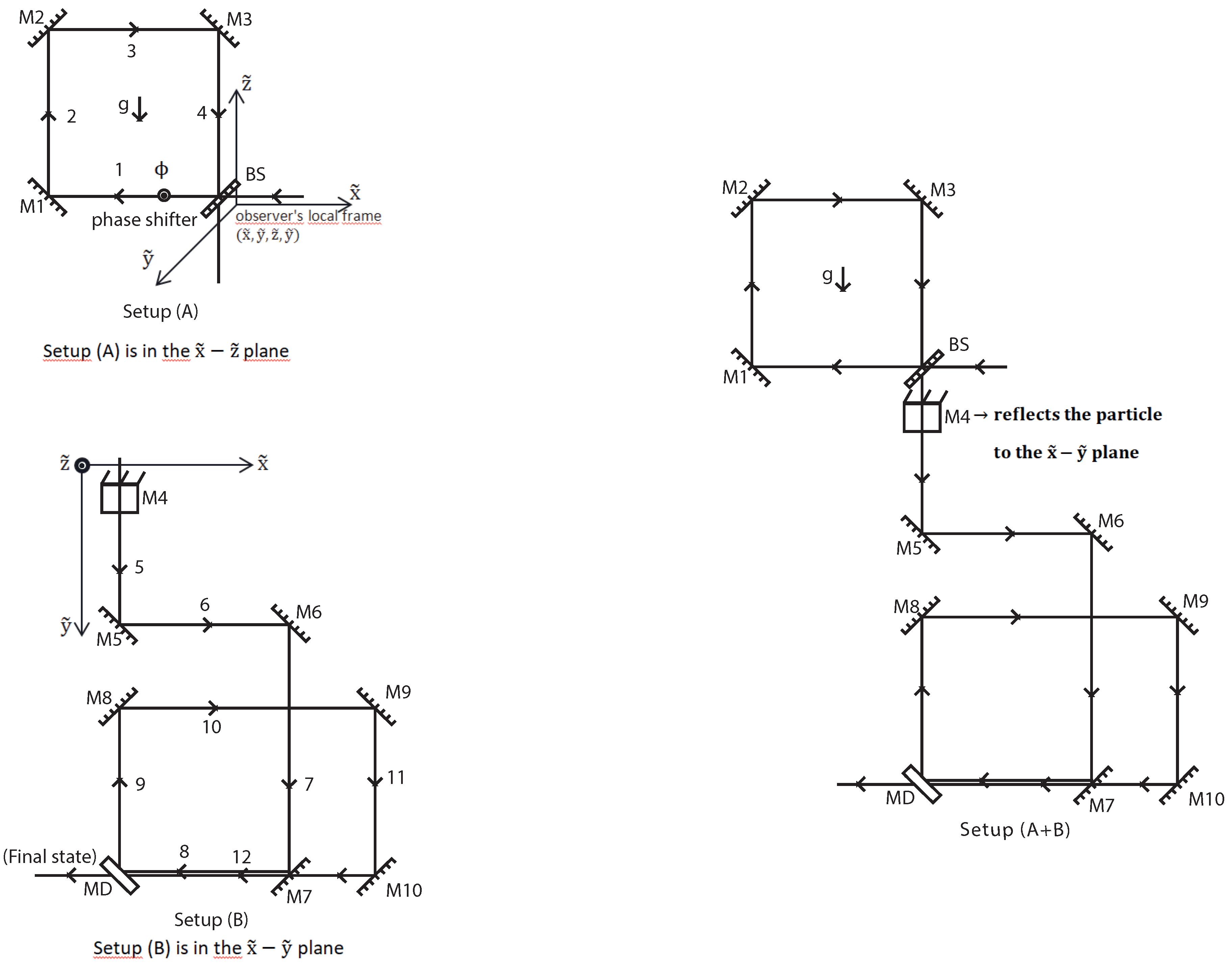
Consider the experimental setup located on the Earth’s surface, shown in Figure A2. The setup is small enough that the gravitational field is assumed to be uniform throughout the setup. Part (A) of the setup is located vertically and the arms at different heights are subjected to different gravitational potentials. On the other hand, part (B) is located horizontally and the arms are at the same gravitational potential. A particle enters the setup through a beam splitter (BS) with adjustable transmission/reflection probabilities. The particle has an evolving internal degree of freedom that can be defined as a "clock". The behavior of a particle with such a clock internal degree of freedom moving in interferometers has been studied previously [13,14]. The setups are in a closed box that the observer cannot see inside. In one corner of the setup (B), there is an apparatus called a mirrored door (MD). The MD acts like a mirror until the observer presses a button. But once the button is pressed, the mirror opens and allows the particle to exit. After waiting long enough, the observer opens the MD by pressing a button and lets the particle out. We assume that the time of flight of the particle on each arm in setup (A) is equal and given by T with respect to the observer’s time. The total flight times along paths 1-2-3-4, 5-6-7-8 and 9-10-11-12 are equal and given by . We define the total motion of the particle in one of these piecewise paths (1-2-3-4, 5-6-7-8 or 9-10-11-12 ) as one revolution. Hence, it takes time for the particle to make one revolution in (A) or (B). The observer presses the button after waiting for a period of , where . The total number of revolutions of the particle in the setup (A) or (B) is determined by the transmission/reflection probabilities of the BS. However, the setup (A) and (B) are at different gravitational potentials. Therefore, how much time the particle spends in which setup (the number of revolutions in setup (A) or (B)) causes the particle’s internal clock to be affected differently by gravitational time dilation. Indeed, the internal clock runs slightly faster in setup (A) than in setup (B). Consequently, when the observer presses the button and opens the MD, she encounters a particle state in superposition of different proper times.
Let us now carry out a quantitative analysis to understand the behavior of the quantum mechanical clock in the gravitational field. The spacetime on the Earth’s surface can be described by the Schwarzschild metric in isotropic form [15].
Here the isotropic coordinate z is related to the radius coordinate of the Schwarzschild metric in standard form as . On the surface of the Earth, it is a good approximation to take ; the difference is of the order of . Define the (Newtonian) gravitational potential as . If the metric (10) is expanded to the series and the terms up to order of are taken into account, we obtain
where is the velocity with respect to the isotropic coordinates and is the proper time, i.e., . However, this velocity is not defined in terms of the local coordinates of the observer on the Earth’s surface. The observer is located on the earth’s surface with its origin on the BS of the setup (see Figure 2). Since the spatial scale of the setup is sufficiently small, it is a good approximation to assert that the velocity of the particle moving through the setup is defined by the local coordinates of the observer. Then, the following relation applies for the magnitude of the local velocity , where R is the radius of the earth. Similarly, the observer writes the Schrödinger equation in her local coordinates () for the metric and describes the quantum mechanical evolution of the particle with this equation. Under this approximation, general relativistic contributions are analyzed in terms of correction terms to the Hamiltonian [13]. In the rest frame of the particle, the evolution of the clock is described by the equation . However, since the time coordinate of the observer is , the evolution of the clock relative to the observer is described by the equation
where,
Here we made use of equation (11) and the definition of local velocity. Note that for , expression (14) gives the gravitational redshift factor between the rest frame of the particle and the local frame of the observer. If the Hamiltonian is expanded into a series and the terms of order and higher are neglected, we get
The multiplier is the gravitational redshift factor between the Minkowski observer at infinity and the local observer at . We prefer to write it as a multiplier since this term is constant and also appears in the Hamiltonian of the particle’s external degrees of freedom. As the rest frame clock Hamiltonian, we use the two-level Hamiltonian
used in ref.[13]. Then, in the rest frame of the particle, the clock state () evolves as
while for a clock moving on the surface of the earth the clock state evolves (according to the Minkowski observer at infinity) as
where is the initial clock state and . It is meaningful to consider the orthogonalization time in determining the period of such a quantum clock. The orthogonalization time of a quantum clock is the minimum time it takes for the clock state to become orthogonal to the initial state [13,16,17]. From (17) and (18) it can be deduced that the orthogonalization time of the clock in the rest frame is
while it is
with respect to the Minkowski observer at infinity. Here we assume that the particle’s velocity is constant along the path. From expression (20) it can be seen that the period of the clock is dilated with respect to the observer at infinity. This time dilation gives both the dilation due to the gravitational potential and the special relativistic time dilation, at the order of the approximation that we have made. If we switch to the coordinates of the local observer on the Earth’s surface, unitary evolution should be carried out using . In this case, the orthogonalization time includes the extra gravitational redshift factor between the observer at infinity and the static observer on the Earth’s surface. The above analysis shows that a quantum clock described by the internal Hamiltonian (16) moving in a gravitational field experiences time dilation just like a classical clock.
Besides an internal clock degree of freedom, the particle also has an external degree of freedom. Let us derive the Hamiltonian describing the particle’s external degrees of freedom. Consider a particle of mass m moving in spacetime described by a static metric. Then, the conserved energy per unit mass is given by
where is the timelike Killing vector [18]. Under the same order of approximation as (15) we obtain the following Hamiltonian
Therefore, relative to a static local observer on the Earth’s surface, the state of the particle evolves as follows:
In the above expression, we adopt a semi-classical approximation for the motion of the particle in the setup. In this approximation, the uncertainty in the position and momentum of the particle is neglected and the positions and velocities (or momenta) in the Hamiltonian are not treated as operators but as numerical functions taking values along trajectories on the arms of the setup. In many experiments with quantum optical interferometers and matter-wave interferometers, a semi-classical approximation is used and particles are assumed to move along certain paths or superpositions of these paths [13,14,19,20]. Without the semi-classical approximation, there is uncertainty in the time of flight of the particle. But if we assume that the experimental setup is of classical scale (the length of its arms is m), then such an uncertainty does not make a significant impact on our results. Using expression (23) and the semi-classical approximation, the final state of a particle that enters from the BS and exits from the MD by making a total of turns, n turns in setup (A) and m turns in setup (B), is given as follows
where
The speed of the particle on paths 2 and 4 is time dependent but on paths 1 and 3 it is constant. The time dependence of the position and velocity must be taken into account when evaluating the integrals in expressions (3.25) and (3.27). In Appendix A we give the time dependences of the position and velocity of the particle moving along different paths. The quantity can be used as a measure of how much the quantum mechanical clock carried by the particle ticks throughout the trip. From (25) and we get
where . The number of tickings of the clock during the trip, is determined from the equation . The term in the argument of the cosine represents the general relativistic time dilation between the setup (A) and (B). Indeed, if , the particle spends all its time in setup (B). In this case the period of the clock is determined only by the term . However, if the particle starts spending time in setup (A) and the time it spends in (A) increases, n will increase and the phase of the cosine will grow. A larger phase of the cosine means a shorter period of the clock relative to the observer. In other words, the phase increases by in proportion to the time the particle spends in (A) and the internal clock runs faster. This is to be expected because in setup (A) the particle is at a higher position in the gravitational field on average.
Now imagine a demon sitting on the particle and recording the ticking of the particle’s internal clock. The demon also keeps a record of the particle’s transmission or reflection from the beam splitter with respect to the proper time. We make one more small adjustment to the setup; let BS allows the particle to cross with 100% probability at the ()th step. Such an adjustment is made to prevent the possibility that there are no particles coming out when the MD is opened after time. Therefore, when the observer opens the MD, she meets the following time state:
In the above expression, we make use of (24) and (25) and . The coefficients are determined by the transmission and reflection probabilities of the BS. Let j be the index indicating the number of reflections or transmissions of the particle in the BS. The index j takes the value . Here indicates the initial particle entering the setup. The jth transmission/reflection probabilities in the BS are defined as follows:
According to these definitions of the probabilities, coefficients are given as
where are real numbers and in the last step was used. From (34) it is easy to deduce the normalization condition
(32) contains time as an intrinsic property in the sense that it contains as a quantum superposition both the different readings of the particle’s clock and the different histories written by the demon based on that clock. Therefore (32) fits our definition of "time state". Note that the demon’s historical records and the time values indicated by the particle’s internal clock are entangled (Both the clock and the records are located on the particle, so they are in approximately the same position. Accordingly, these entangled systems are not separated in a space-like manner.). A measurement of the reading of demon’s historical records also provides a measurement of the reading of the proper time value indicated by the clock. There is one more subtle issue we would like to draw attention to. In the context of kinematic relativity, arbitrariness in clock synchronization has been well known since Reichenbach [21] and Grünbaum [22]. It is therefore important to realize that the difference in clock readings is not a matter of convention, but is due to a change in the duration at which the clock ticks. Indeed, all clocks in superposition have the same initial synchronization given by .
We need to be precise about how the demon keeps the historical records. What interests us in a PBR-type proof is not all the demon’s records, but only the records concerning the particle’s n number of turns in the setup (A). We therefore index the records with n. As in Section 2, we assume that the demon’s recordings are recorded on a quantum mechanical system. He uses qubits instead of classical bits. One way to record in this way is to convert the number n to binary and take the tensorial product of the qubit states. For example, for , is denoted by , by ,..., by . However, we would like to point out that in our PBR-type proof we only need to consider the case . This is because we only need to prove the physicality of time represented by 1 qubit of information.
By varying the transmission/reflection probabilities of the BS for a fixed number N, we can prepare distinct states with different proper time superpositions. Let and be two such distinct states with reflection/transmission probabilities and respectively. Suppose we perform M uncorrelated preparations from states and . Then the prepared systems are brought together for measurement. Depending on which of the two preparations is employed each time, M systems are prepared in one of the following quantum states:
where, . Since the preparations are independent, the complete physical state of the systems prepared by the setups is compatible with any of these quantum states with non-zero probability at least . Indeed, assuming that time is epistemic, there exist two quantum states and such that . For these states, the ontic state lies at the intersection with a non-zero probability q. If it is deduced that there is a joint measurement on this M system such that each outcome has probability zero on at least one of the states of (36), then a contradiction is obtained. Thus, by reductio ad absurdum time is proven to have ontological reality.
As we discussed before, we just need to show the contradiction for . If we take in equation (32) and choose for the phase shifter in setup (A), then we get
where and . Here, and are transmission probabilities (33) for preparations indexed by 0 and 1. The Hilbert space for (37) is the four dimensinal space . We index the record states with the subscript "rec" to distinguish them from the qubit states of the clock. Let us define the following unitarity operator on
where
It is shown in Appendix B that the probability of the following measurement on states (36) yields zero:
where,
Here, is the identity operator on the Hilbert space and the operator denotes the transformation performed by the quantum circuit used in the PBR paper (see Figure 3 of ref.[1]). In our paper operator acts on the Hilbert space . and represent the basis vectors of and respectively. The equation (42) reveals a contradiction between the assumption that time is epistemic and the predictions of quantum theory. Accordingly, if the predictions of quantum theory are correct, then time cannot be an epistemic property.
4. Conclusions
It is worth discussing the presuppositions under which we prove that time has ontological reality. First of all, our proof presupposes the PBR assumptions. Accordingly, the existence of an observer-independent real physical state is assumed, such that systems prepared independently have independent physical states. PBR makes this assumption for systems that are not entangled with other systems. However, in the time states we use in our proof, there is entanglement between the clock and the record states, as seen from equation (32). Thus, we assume entanglement, albeit not between two space-like separated systems. On the other hand, this does not weaken our proof. Because our aim is not to prove the physicality of the quantum state and, consequently, that quantum probabilities are not a matter of information. The PBR has already proven this result. What we prove is that the novelty brought by quantum probabilities can generate "time" in the context of general relativity. Thus, time in the sense of the novelty inherent in quantum probabilities and the notion of time in physics are to some extent converging. To arrive at this conclusion, quantum theory and general relativity need to be handled together. In a simple tabletop experiment, and of course under certain approximations, we have defined the time state by combining the predictions of these two theories; in this way, we have treated these two theories together. We have shown that quantum probabilities are capable of generating time, associated records and history determined by a quantum mechanical clock moving along a world line. Of course, we reached this conclusion through a gedankenexperiment designed on a very specific system. Therefore, it can be argued that the generation of time by quantum probabilities cannot occur as a result of natural processes, but only under some special conditions. On the other hand, the existence of spacetime superpositions on a very small scale is a prediction of quantum gravity theories [23,24]. It follows that quantum probabilities generate an ontic notion of time at a fundamental level in nature.
In addition to the PBR presuppositions, we have another assumption, which we call the universality of quantum probabilities. This assumption assumes that the time generated by quantum probabilities is the same regardless of which system or preparation the probabilities come from through the reduction of quantum superposition. Accordingly, a simple bipartite quantum superposition state is a typical state encoding time. It follows that the PBR-type proof only needs to consider these typical states. This assumption also implies that each small piece of time is identical in nature to every other small piece, i.e., each small piece of time has the same genetics as the whole. This is important since it shows that a long interval of time resulting from successive state reductions is not different in nature from a small interval of time resulting from a single reduction. Such a notion of time, resulting from the quantum probabilities introduced by state vector reduction, is not something that flows continuously; rather it is a set of discrete little chunks of time. Is there an ordering on this set? In other words, can the arrow of time be defined? The issue is worth discussing. The quantum probabilities arise from the reduction of a superposed quantum state. The fact that these probabilities have no epistemological origin, then, has to do with the fact that quantum superpositions have physical reality and state reduction is a physical process (As concluded in ref.[1], if the quantum state is a physical property of a system then the state vector reduction must correspond to a physical process.). The state vector reduction is a process in which information destruction takes place [25]. Therefore, if one accepts that reduction is a physical process, then there must exist a non-epistemic arrow for time. On the other hand, an isolated quantum system evolves unitary and returns to its initial state infinitely often, at least if the number of incommensurable energy levels is not too small [26,27]. Accordingly, quantum dynamics alone does not provide an arrow for time unless the reduction of the state vector is taken into account. The situation does not change significantly even in open quantum systems where the system interacts with its environment. Correlations resulting from the interaction of the quantum system with its environment lead to an exponential decay of the off-diagonal elements of the density matrix and decoherence occurs [28]. However, there is no loss of information during decoherence; Information is transferred from the system to the environment. Although the exponential damping eliminates the macroscopic interferences, the diagonal terms of the density matrix are not affected. Some authors have argued that fluctuations in channel probabilities occur due to fluctuations in the environment and that this can lead to reduction, i.e., these fluctuations provide one of the channel probabilities to be 1 [29]. Even if one accepts that such an explanation based on quantum principles for state vector reduction is correct, it does not give us a (non-epistemic) arrow of time. Indeed, in this case, quantum probabilities are related to the information stored in the environment, that is, the information that has flowed from the system into the environment and the information of fluctuations in the environment. On the other hand, the process of state reduction, often interpreted as information destruction, produces an irreversible sequence of new events, in contrast to decoherence-based explanations. This sequence of irreversible events defines an ontic arrow for time.
Appendix A. The Time Dependencies of the Position and Velocity of the Particle Moving along Different Paths
The gravitational field is assumed to be constant throughout the size of the experimental setup. Accordingly, on the paths 2 and 4 of the setup (A), the particle moves with constant acceleration, while on the paths 1 and 3 it moves with different magnitude but constant speed. The speed of the particle on all paths in setup (B) is constant and equal to its speed on path 1. The potential difference between paths 1 and 3 is so the potentials for these paths are
The velocity of a particle accelerating with a constant proper acceleration g and its position component in the direction of acceleration is given by [30]
where the initial velocity and acceleration are assumed to be parallel. Since the origin of the observer’s local frame coincides with the BS on path 1, the initial position for path 2 is and for path 4 is , where h is the height between paths 1 and 3. For a particle traveling on paths 2 and 4, we give the velocity and position functions for the sake of completeness:
The constant speed of the particle on path 3 is . Recall that T is the flight time of the particle on each path relative to the observer. The potentials to which the particle is subjected for its motion on paths 2 and 4 are
Appendix B. Derivation of the Equation (42).
It can be easily deduced that the effect of the operator (38) on the states (37) is of the form
where
In the expression above and . Therefore,
where and . From the above equation and definition (44) we obtain
Here operator performs the transformation described by the quantum circuit of ref.[1], i.e.,
It was proved in ref.[1] that for any M chosen large enough that , it is possible to choose the real parameters and such that (A12) is zero.
Figure A1.
The tapes, each containing N qubits, are prepared independently in one of the quantum states where or 1. The prepared M systems are brought together for measurement.
Figure A1.
The tapes, each containing N qubits, are prepared independently in one of the quantum states where or 1. The prepared M systems are brought together for measurement.
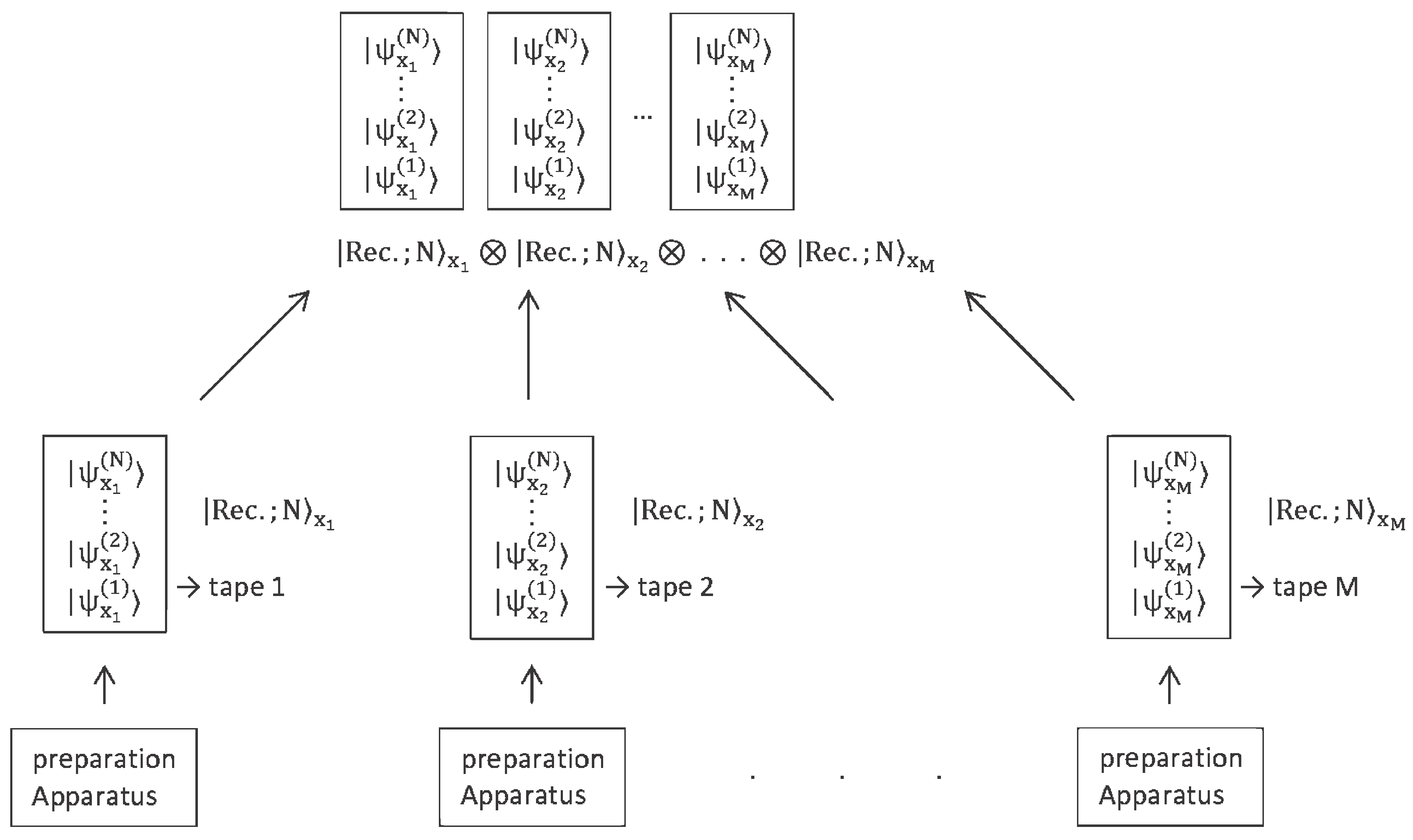
Figure A2.
Scheme of experimental setup located on the Earth’s surface. BS represents beam splitter, ,.., represent mirrors and MD represents the mirrored door which acts like a mirror until the observer presses a button. But once the button is pressed, the mirror opens and allows the particle to exit. The experimental setup consists of parts (A) and (B). On the left panel, parts (A) and (B) are shown separately and on the right panel the complete setup is shown as a whole. Part (A) of the setup is located vertically and the arms at different heights are subjected to different gravitational potentials. Whereas part (B) is horizontally located and the arms are at the same gravitational potential. The mirror is located very close to the BS (the BS- distance is neglected during calculations) and reflects the particle in the plane to the plane, ensuring that the setup (B) is in the horizontal plane with respect to the gravitational field . The origin of the observer’s local frame is placed on BS. The time of flight of the particle on each path in setup (A) is equal and T relative to the observer’s time. The total flight times along paths 1-2-3-4, 5-6-7-8 and 9-10-11-12 are equal and given by , so we say that the period of each revolution is relative to the time of the observer.
References
- Pusey, M., Barrett, J. and Rudolph, T. On the reality of the quantum state. Nature Phys 8, 475–478 (2012). [CrossRef]
- Barbour, J. The End Of Time, Oxford University Press, Oxford, 1999.
- ’t Hooft, G. The Free-Will Postulate in Quantum Mechanics. quant-ph/0701097.
- Scardigli, F., ’t Hooft, G., Severino, E., Coda, P. Free Will in the Theory of Everything. In: Determinism and Free Will. Springer, Cham. (2019).
- Conway, J. and Kochen, S. The Free Will Theorem. Found. Phys. 36, 1441-1473 (2006). [CrossRef]
- Conway, J. and Kochen, S. The Strong Free Will Theorem. Notices AMS 56, 226-232 (2009). [CrossRef]
- Acín, A., Masanes, L. Certified randomness in quantum physics. Nature 540, 213–219 (2016). [CrossRef]
- Herrero-Collantes, M. and Garcia-Escartin, J. C. Quantum random number generators. Rev. Mod. Phys. 89, 015004 (2017). [CrossRef]
- Senno, G., Strohm, T., and Acín, A. Quantifying the Intrinsic Randomness of Quantum Measurements. Phys. Rev. Lett. 131, 130202 (2023). [CrossRef]
- DeWitt, B. S. Quantum mechanics and reality. Physics Today 23, 9, 30 (1970).
- Harrigan, N., Spekkens, R.W. Einstein, Incompleteness, and the Epistemic View of Quantum States. Found Phys 40, 125–157 (2010). [CrossRef]
- Gödel, K. A remark about the relationship between relativity theory and idealistic philosophy (1949a), in Solomon Feferman, and others (eds), Collected Works: Volume II Publications 1938-1974 (New York, NY, 2001; online edn, Oxford Academic, 31 Oct. 2023),.
- Zych, M., Costa, F., Pikovski, I. and Brukner, Č. Quantum interferometric visibility as a witness of general relativistic proper time. Nat Commun 2, 505 (2011). [CrossRef]
- Zych, M., Pikovski, I., Costa, F. and Brukner, Č. General relativistic effects in quantum interference of “clocks”. J. Phys. Conf. Ser. 723, no.1, 012044 (2016).
- Weinberg, S. Gravitation And Cosmology, John Wiley and Sons, New York, 1972.
- Mandelstam, L. and Tamm, I. The uncertainty relation between energy and time in non-relativistic quantum mechanics. Journ. Phys. USSR 9, 249-254 (1945).
- Fleming, G. N. A unitarity bound on the evolution of nonstationary states. Nuovo Cim. A 16, 232–240 (1973). [CrossRef]
- Carrol, S. M. Spacetime and Geometry An Introduction to General Relativity, Addison Wesley, San Francisco 2004.
- Pikovski, I., Zych, M., Costa, F. et al. Universal decoherence due to gravitational time dilation. Nature Phys 11, 668–672 (2015). [CrossRef]
- Overstreet, C., Asenbaum, P. and Kasevich, M. A. Physically significant phase shifts in matter-wave interferometry. Am. J. Phys. 89, 324–332 (2021). [CrossRef]
- Reichenbach, H. The Philosophy of Space and time, Dover Publications, New York 1958.
- Grünbaum, A. Philosophical problems of space and time, Alfred A. Knopf, New York 1963.
- Rovelli, C. Quantum Gravity, Cambridge University Press, 2004.
- Christodoulou, M. and Rovelli, C. On the possibility of laboratory evidence for quantum superposition of geometries. Physics Letters B 792, 64–68 (2019). [CrossRef]
- von Neumann, J. Mathematische Grundlagen der Quantenmechanik, Springer, Berlin 1932; English Translation by Beyer, R.T. Mathematical foundations of quantum mechanics, Princeton University Press, Princeton 1955.
- Hogg, T. and Huberman, B. A. Recurrence Phenomena in Quantum Dynamics. Phys. Rev. Lett. 48, 711 (1982). [CrossRef]
- Peres, A. Recurrence Phenomena in Quantum Dynamics. Phys. Rev. Lett. 49, 1118 (1982). [CrossRef]
- Zurek, W. H. Environment-induced superselection rules. Phys. Rev. D 26, 1862 (1982). [CrossRef]
- Omnès, R. Decoherence and wave function collapse. Found. Phys. 41, 1857 (2011). [CrossRef]
- Styer, D. F. How do two moving clocks fall out of sync? A tale of trucks, threads, and twins. Am. J. Phys. 75, 805 (2007). [CrossRef]
Disclaimer/Publisher’s Note: The statements, opinions and data contained in all publications are solely those of the individual author(s) and contributor(s) and not of MDPI and/or the editor(s). MDPI and/or the editor(s) disclaim responsibility for any injury to people or property resulting from any ideas, methods, instructions or products referred to in the content. |
© 2024 by the authors. Licensee MDPI, Basel, Switzerland. This article is an open access article distributed under the terms and conditions of the Creative Commons Attribution (CC BY) license (http://creativecommons.org/licenses/by/4.0/).
Copyright: This open access article is published under a Creative Commons CC BY 4.0 license, which permit the free download, distribution, and reuse, provided that the author and preprint are cited in any reuse.


