
Submitted:
25 March 2024
Posted:
26 March 2024
You are already at the latest version
Abstract
Quantum physics is intrinsically probabilistic. The entropy of a quantum state quantifies the amount of randomness (or information loss) of such state. The degrees of freedom of a quantum state are position and spin, and upon their specification Born's rule in phase space defines randomness. We focus on the spin degree of freedom and elucidate the spin entropy. Then, we present some of its properties and show how entanglement increases spin entropy. Some speculative predictions on the decay of the $Z^0,W^{+,-}$ gauge bosons conclude the paper.
Keywords:
Spin Entropy
; Phase Space
; Quantum Information
; Entanglement
; Geometric Quantization
1. Introduction
This paper addresses the problem of quantifying the randomness associated with a spin state. Our broader motivation is to study the role of randomness in quantum physics. We follow the Geometric Quantization method (GQ) [1,2,3,4,5] a formulation of quantum physics derived from classical physics in phase space. One can then view quantum physics as embedding randomness into phase space classical physics and so seeing it as an information theory. Previous work addressed information theory aspects of quantum physics, see [6,7,8,9,10,11,12,13,14,15,16] and their references. We point out the GK-Law[15], a hypothesis that in a closed physical system information cannot be gained. Thus, the entropy of a quantum state could and should play a role in helping us make predictions about particle physics.
The degrees of freedom (DOFs) of a quantum state are associated with the position and spin values of a particle, i.e., all randomness of a quantum state is captured by Born’s rule once the DOFs are specified as well as its phase space. Thus, our attempt to capture the information content of a quantum state, must address these degrees of freedom as well as their phase space. We point out that in quantum physics, von Neumann entropy [6] quantifies only the lack of knowledge an observer has about a quantum state, i.e., it quantifies only the randomness in specifying its DOFs. Thus, for all pure states, von Neumann entropy is zero, while our entropy formulation is focused on pure states.
With respect to the position DOF Geiger and Kedem [15] formulated the x-p phase space quantum entropy. Let us then focus on the spin DOF.
Note that quantifying the randomness of the spin state along the z-direction alone is not sufficient, since a measurement of an eigenstate of is certain to yield the eigenvalue of this eigenstate, and yet there is the randomness associated with any spin measurement in the x-y plane as demonstrated by the Stern-Gerlach experiments[17]. It is in the spin phase space where all the randomness of a spin state is captured.
Historically, spin was first conceived as a quantum concept, but GQ derives it as the quantization of the classical two-sphere . In this Hilbert space two independent variables, such as the zenith and azimuth angles, and respectively, are required to specify a spin wave function . These classical variables are associated with the polarization of spin particles. Not only does GQ produces a description for the spin, originated from classical ideas, but also provides the spin phase space where the wave function and all its randomness is defined.
The information content, or lack thereof, associated with the phase space wave function is captured by the differential entropy [18], i.e.,
We will refer to (1) as spin-entropy. While many of the properties exhibited by the spin-entropy also hold for the more general Rényi entropy of order given by
we focus on the spin-entropy in this paper.
1.1. Previous Work
Wehrl entropy [19] was introduced to approximate a classical entropy for a quantum state, and Lieb studied spin-coherent states to evaluate Wehrl spin entropy [20,21,22] As in the case of spatial coherent states, spin coherent states constitute an overcomplete set of states. Since Werhl entropy is based on an overcomplete basis representation, projections onto this basis lead to quasi-probabilities violating the Kolmogorov third axiom. The overcomplete basis decomposition and the arbitrariness of the choice of spin-coherent states basis to define the probability distribution prevent Wehrl entropy from accurately quantifying the randomness associated with the spin observables.
This work does start from a similar view as [23] and here we steer it differently, correcting their attempt to decompose the wave function in phase space.
1.2. Paper Organization
The paper is organized as follows: Section 2 provides a summary of GQ concepts, based on [5], applied to the sphere and focus on a derivation of the wave function in spin phase space. Extensions to these GQ concepts are also in the Appendix A and references. Section 3 derives the main spin-entropy properties, including a formula for all the eigenstates of the z-direction for any spin s. Section 4 analyzes the connection between phase space entanglement and spin-entropy. We show that the more the entanglement between two particles the larger is the spin-entropy. Section 5 concludes the paper with speculations about the role of spin-entropy in particle physics.
2. Some Geometric Quantization Concepts
We first provide a summary of concepts used in this paper developed by the GQ of the two-sphere to describe spin operators and eigenfunctions in phase space. Some extra material to complete the descriptions presented in this summary is presented in the Appendix A.
2.1. Complex Plane and the Sphere
Consider the local variable to describe the complex plane . The stereographic projection of the 3D embedding of the sphere of radius s via the south pole , to the plane is given as
where are the zenith and azimuth spherical angles, respectively. The inverse mapping is then given by
and the mapping of the south pole to z requires the stereographic projection via the north pole, i.e., .
2.2. Symplectic Structure for the Sphere and Canonical Transformations
A symplectic structure for the sphere manifold is given by
where is an integer. Canonical transformations preserve . Consequently for vector fields to be generators of canonical transformations in the sphere, the transformation must satisfy
Thus, for every infinitesimal canonical transformation we can associate a function J on such that is a closed one form. Also, by inverting we get
Thus, conversely, given a classical observable J the generators of the infinitesimal canonical transformation can be readily obtained.
2.3. Spin Operator and Eigenfunctions
In order to derive the spin operators one consider the classical functions , , in the sphere, as described by (2.1). The generators of the canonical transformations associated with these functions, derived from (2.2), are isometries of the sphere. In Appendix A we give a summary of the GQ steps to obtain the quantum operator operators (A.3) acting on the two-sphere associated to these functions . These are the spin operators and can then be written as
The eigenfunctions of the operator (due to the polarization condition, see appendix (A.3), (A.3)) are of the form
which leads to
with solutions of the form
where and we note that compare to the presentation of Nair[5] the functions do have an extra factor for normalization purposes. In the representation (2.1) the wave function (2.3) is written as
These wave functions form an orthonormal basis, i.e.,
Then, through linear superposition of these eigenstates, all spin-wave functions in phase space for spin s are constructed.
Note that a wave function in the x-p phase space is decomposed as a product of a wave function on x and a wave function on p, related to each other by the Fourier transform. In contrast, a wave function in the spin phase space cannot be “reduced”, i.e., cannot be decomposed as a product of wave functions where each contains just one variable of phase space. Instead, a wave function over the entire spin phase space, the entire sphere, is required.
3. Spin-Entropy in Phase Space
Lemma 1
(Space Homogeneity). The spin-entropy, given by (1), is invariant under rotations and reflections of the coordinate system.
Proof.
Given a function , define a functional on the sphere
where .
The spin-entropy is one such functional for the function
Consider an isometry transformation , so . Applying an isometry to the wave function , i.e., applying it to g leads to
where we used the fact that isometries of the sphere are canonical transformations that preserve the symplectic form, i.e., the determinant of a Jacobian of a canonical transformations is 1, i.e., .
Thus the spin-entropy is invariant under isometries. The isometries of the sphere are the three reflections, and combinations of two reflections gives the rotations. □
One immediate conclusion is that the homogeneity of the space is reflected by the invariance of the spin-entropy to rotations and reflections of the coordinate system. So given a spin-state associated with and such that for some choice of z-coordinate it has , this state will have a spin-entropy value regardless if one chooses or not this z-coordinate to describe it.
Let us consider the eigentstates along the z-direction, described by (2.3). The spin-entropy (1) associated with these eigenfunctions is
where the probability normalization constant is given by and .
For the rest of this section, and for manipulation purposes, let us define the integer variables and , and since , we have . We may refer to as it is more convenient during manipulations.
Lemma 2
(Spin-Entropy Formula for z-Eigenstates). The spin-entropy in phase space for the z-eigenstates is invariant under the reflection and can be written as
where is the heaviside function, i.e. for and for .
Proof.
Following on (3), let us first proceed to evaluate the spin-entropy. We will refer to as the spin-entropy of the eigenstate and refers to the normalization . We then write (3) as
where
and in the last step we applied the transformation .
Noting that , it is then clear that the spin-entropy (3) have the property . And since the transformation is equivalent to , we obtain that to conclude the first statement of the lemma.
In order to evaluate define
Thus,
Considering the Ansatz that . Then, the case is already solved in (3), i.e., . We can then advance (3) for by a recursive method
Replacing and into (3) concludes the lemma. □
The entropies for the special cases and are readily derived
Lemma 3
(Spin-Entropy Variation Across z-Eigenstates). Let be the z-eigenstates of spin s. Let represent m restricted to the range , i.e., . The spin-entropy decreases as increases. Moreover, the decrease in as one vary from to is given by
Proof.
Adopting the notation we can rewrite the last two terms in (2) as
where is the heaviside function, i.e., for and otherwise. Consider the difference of consecutive values of the spin-entropy described by (2) for , i.e.,
For the last step we used Lemma 8. □
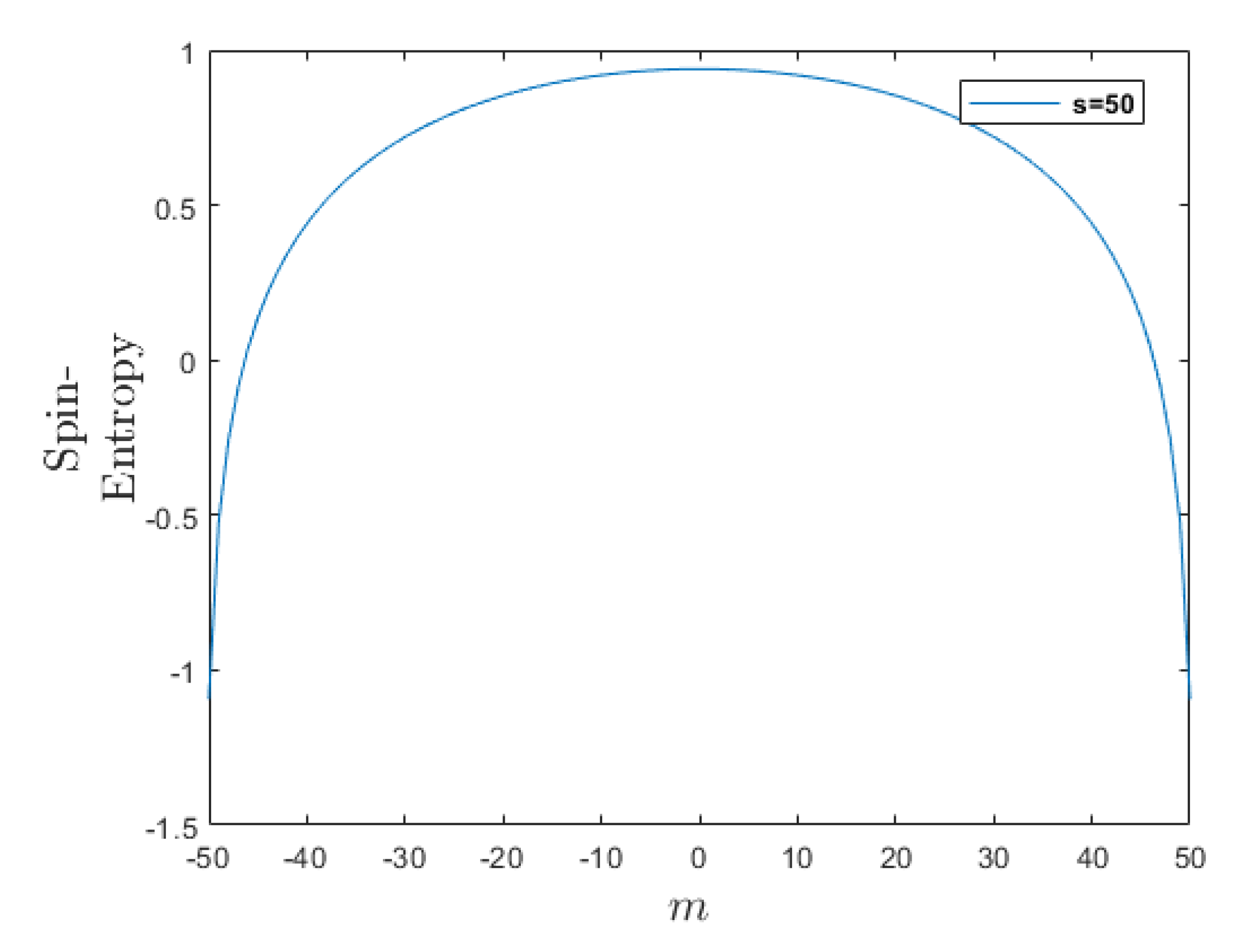
Figure 1.
Spin-Entropy for eigenstates along z-direction. It is invariant by transforming and it is decreasing as m increases in the range (see Lemma 3).
Figure 1.
Spin-Entropy for eigenstates along z-direction. It is invariant by transforming and it is decreasing as m increases in the range (see Lemma 3).
Lemma 4
(Negative Spin-Entropy across z-Eigenstates). Let be the z-eigenstates of spin s. For the spin-entropy of to have a negative value it is required that .
Proof.
From Lemma 3 the lowest entropy of a spin s particle is attained for . Examining the the spin-entropy formula (2) for such cases and requiring it to be negative we get
and since s must be a multiple of , the minimum value of s for which this is possible is . □
Since the visible universe does not seem to contain particles with spin , such mathematical property may not be relevant to physical systems. Let us examine some properties of spin and for all spin states.
3.1. Spin One-Half
Lemma 5
(Spin Entropy). All spin states have the same spin-entropy
Proof.
Let us refer to as an arbitrary spin-state. All spin states are reached by the application of an element of the to .
There exists a two-to-one homomorphic mapping of the group onto the group . If maps onto , then . This implies that the representations of are also representations of .
By Lemma 1 we conclude that all spin-states will be reached by a canonical transformations of any given spin-state and therefore have the same spin-entropy. □
3.2. Spin One
Lemma 6.
The maximum value of the spin-entropy for is and it is reached by the state and all its canonical transformations (rotations and reflections). The minimum value of the spin-entropy for is and it is reached by the states and and all their canonical transformations (rotations and reflections).
Proof.
The probability density does not depend to the global phase term and thus, the spin-entropy vary according to the four parameters . Note that for a given a set of these parameters all canonical transformations (rotations and reflections) of this wave function will correspond to transformations in parameter space.
For example for the canonical transformation of a rotation around the z-axis we have and the wave function (3.2) is then written as
corresponding to a translation in the parameters .
The rotations have three degrees of freedom and thus, the space of parameters that cause the spin-entropy to vary is reduced to one. This degree of freedom still have a reflection to reduce it further by one half the possible variations of the spin-entropy values. Thus, we examine the wave function restricted to varying one parameter.
Consider the spin-1 state (3.2) for the case of and , i.e.,
where is the free parameter. All canonical transformations of such state lead to the same spin-entropy distribution. The probability is then
where . The spin-entropy of this state is
The extremes of the entropy occur when , i.e., when
They occur for . By investigation, the cases are the z-eigenstates and yield the minimum spin-entropy. The cases are associated with the x-eigenstates and y-eigenstates, , respectively, i.e., they are canonical transformations of the z-eigenstates, and yield the maximum spin-entropy. □
We show in Figure 2 a simulation for this spin-entropy as vary.
Note that the state have a higher spin-entropy than the states , i.e., there is more randomness and less information at the state. The GK-law [15] says that the arrow of time in quantum physics, for a closed system, is given by an increase in quantum entropy. If GK-law holds and if the laws of conservation allow, then transition from a spin-state to the spin-state can occur. However, a transition from a spin-state to either of the spin-states cannot occur.
In order to test such hypothesis, one may investigate , bosons of , where such phenomena or lack thereof would be observed. These particles decay quickly (usually attributed to their large masses) and we speculate the trigger may be due to these forbidden transitions. More precisely, the state (3.2) is a superposition of z-eigenstates and and oscillates as vary. At its maximum spin-entropy the state is either the x-eigenstate () or the y-eigenstate (). The spin-entropy (3.2) will also oscillate as vary following the same cycle as the state probability (3.2). For varying over time (due to the quantum Hamiltonian) the spin-entropy would oscillate and if the GK-law holds, these particles decay would be a mechanism to bar the spin-entropy from decreasing.
Conjecture 1.
The spin-entropy associated with any spin state of magnitude s has its maximum value for the states and all its canonical transformations. The spin-entropy associated with any spin state of magnitude s has its minimum value for the pair of states and all its canonical transformations.
We have shown to be true for the cases of and and . Also, by Lemma 3 the z-direction eigenstates, for any s value, will have lower spin-entropy the larger is. All canonical transformations of a state will have the same spin-entropy. It remains to be proven that any spin state will have the spin-entropy between these values or that the extremes of the spin-entropy occur for the spin-eigenstates.
4. Phase Space Entanglement Increases Entropy
Following [7,8,24,25,26] and their references, let us define the entanglement of these two orthonormal spin eigenstates as
where controls periodically the amount of entanglement. With minimum (no) entanglement occurring at and maximum entanglement occurring at .
By Born’s rule this spin-state has a probability density
The spin-entropy of state (4) is
The extremes of the entropy occur when , i.e., when
We conjecture that they occur for . By investigation of these four cases, the cases , associated with no entanglement, yield the minimum spin-entropy which is the sum of the spin-entropy of each state. We have already calculated each state spin-entropy in (2). The cases yield the maximum spin-entropy and are associated with maximum entanglement.
We present "a sketch of a proof" by reasoning about randomness. Let us examine the role of each of the wave functions, and , that are being entangled (4). Each represent a distribution in a two-sphere , or let us call it a “container”. The phase space of the entanglement is the product of these two “container”. For , when there is no entanglement, despite the phase space being the product of two “container”, each of the distributions occupies only one of the containers. Thus, the entanglement spin-entropy is the sum of the spin-entropy of each container. For , when there is maximum entanglement, the wave functions occupy equally both containers, i.e., they are mixed in the containers. The more spread is a distribution the larger is the entropy. The parameter controls the mixture, and so the more is the mixture the larger is the spin-entropy. This reasoning is not specific about spin entanglement, it also applies to position entanglement.
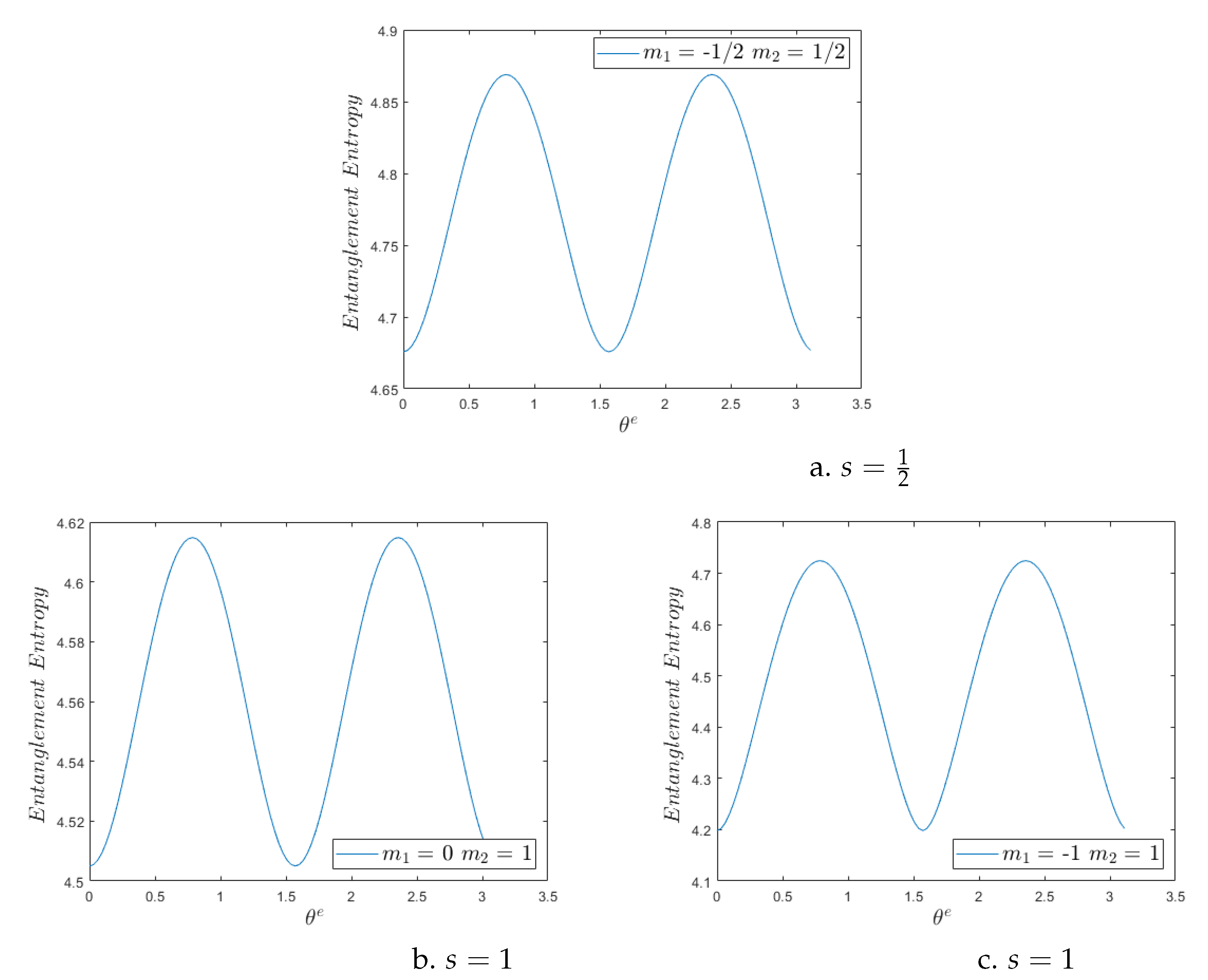
In Figure 3 we plot the spin-entropy (4) vs for z eigenstates of and for z eigenstates of . Clearly, spin-entropy increases as the entanglement increases. It is noticeable that the spin-entropy of the entanglement , for any given , is larger than the spin-entropy for the same of any of the possible entanglements for . For the case , the cases b. has the same entanglement entropy as the case . This can be inferred from the mapping , i.e., the mapping lead to the same probabilities (4) and thus, to the same spin-entropy (4). Comparing the cases b. with c. , it is noticeable that it is for c. that the minimum entanglement value as well as the maximum entanglement value occurs. The minimum entanglement is the product states and so the spin-entropy is simply the sum of the spin-entropy of both states, thus c. is smaller. The maximum value of the spin-entropy being awarded to c. is of interest. We wonder if it maybe related to the fact that the superposition of these two states is a canonical transformation of the higher entropy state , see Figure 2.
5. Conclusion
This paper quantified the randomness associated with a spin state by defining the spin-entropy in phase space.
At the formal level we used differential entropy from information theory and the Geometric Quantization method (GQ) applied to the two-sphere. The GQ produces a description for the spin, originated from classical ideas, and also provides the spin phase space where the spin-wave function and all its randomness is defined. Local canonical transformation in phase space preserve the area element of the sphere and guarantees the spin-entropy satisfies the homogeneity hypothesis, and so Lemma 1 showed the spin-entropy of a spin state is invariant under 3D rotations and reflections of the coordinate system.
Lemma 2 provides a spin-entropy formula for the z-direction spin-eigenstates. Lemma 3 and a plot of the spin-entropy of a given spin s versus different values of , see Figure 1, showed that the spin entropy is symmetric with respect to , and decreases as m increases for . Thus, in particular, the state has a higher spin-entropy than the spin states , i.e., there is more randomness and less information at the state.
If the GK-Law [15] holds, i.e., the arrow of time in quantum physics is given by an increase in quantum entropy for closed systems, and if the laws of conservation allow, then a transition from a spin-state to a spin-state can occur. However, a transition from a spin-state to either of the spin-states cannot occur. In order to test the GK-Law, one may investigate , bosons of , where such phenomena or lack thereof would be observed. We speculate that their fast decays, with a half-life of about s, are triggered by oscillatory behavior of a superposition of their eigenstates (see Figure 2 with the interpretation that the parameter is varying with time, thus the oscillations) coupled with the GK-Law of an impossibility of transitions from . After all, if a transition is forbidden and in order to bar the spin-entropy to decrease, then a mechanism to avoid this event, and satisfying the conservation laws, is to annihilate such particles and create new particles.
The phase space of the entanglement of two states is the product of two phase spaces. We reasoned that the entanglement correspond to a distribution that mixes the two phase spaces while the product of states does not mix. The larger is the entanglement, the more is the mixture, the more randomness, and so the larger is the entropy. We speculate that the phenomena of decoherence [7,8,24,26,27] of a subsystem immersed in an environment occurs so that parts of such subsystem will entangle with the environment and the total entanglement increases. An interesting future direction could exploit a connection of this work to the work on quantum thermalization [10,28,29,30] and their references, where they suggest a procedure that by tracing out the environment and evaluating the reduced density matrix of a system of interest may lead to the entropy of classical physics.
Acknowledgments
I want to thank professor C. Tomei for showing me the simple and elegant demonstration of Lemma 1. I want to thank professor P. Nair for his notes and patience in teaching me various aspects of the Geometric Quantization method as well as suggestions for studying the spin-entropy properties. I want to thank professor Z. Kedem for providing feedback in the early manuscript. I want to thank Dries Sels for many interesting conversations and pointing out to me various work on quantum information. This paper is partially based upon work supported by both the National Science Foundation under Grant No. DMS-1439786 and the Simons Foundation Institute Grant Award ID 507536 while the first author was in residence at the Institute for Computational and Experimental Research in Mathematics in Providence, RI, during the spring 2019 semester “Computer Vision” program.
Appendix A Geometric Quantization Summary
Here we cover some topics considered by geometric quantization when applied to the two-sphere to create the spin operators and wave functions. For more in depth view of the method see [3,4,5]
Appendix A.1. Symplectic Structure
Considering the symplectic structure to be the oriented surface area element of a sphere scaled down by the radius s, it is written as
This symplectic structure can be derived from a Kähler potential where
and is an integer associated with a spin magnitude s. The symplectic potential has the components given by
Here we abused the notation that , when used as superscript or subscripts, do represent the index of the component of a vector. A special case occurs for which represents both, the index of as well as the variable for which the partial derivative is differentiating. We may also switch to the component notation to indicate and , which will help with manipulations. In this case we may represent the vector potential by . We will use both notations.
The corresponding covariant derivatives are
Appendix A.2. From Canonical Transformations to PreQuantum Operators
Canonical transformations preserve . Consequently for the vector fields to be generators of canonical transformations in the sphere, written as , must satisfy (derived in (2.2)). Thus, for every infinitesimal canonical transformation we can associate a function J on such that is a closed one form.
The symplectic potential change under a canonical transformation is given by
Thus, under a canonical transformation , where . The symplectic potential may be thought of as a (1) gauge field, with the transformations . In order for to be a covariant derivative under canonical transformation the wave function must transform as . This form of the canonical transformation of will lead to the unitary operators associated with observable J.
Consider a function in phase space generating a canonical transformation and described by the change of the symplectic potential . The corresponding change in is thus
Thus, associated to the classical function the GQ method creates the prequantum operator for the classical observable J
and so canonical transformations are implemented as quantum unitary transformations of the wave function, .
Appendix A.3. From 3D Embedding Functions to Quantum Spin Operators
Let us refer to the 3D embedding in the sphere (2.1) as the “classical spin variables” for which the quantum spin operators will be derived as follows. From these variables we can evaluate the canonical transformations (2.2) for the symplectic (2.2) or its inverse, i.e., we can obtain the Hamiltonian vector field coefficients
Similarly to the abuse of notation of , the abuse of notation to the 3D variables occurs when using them as superscripts or subscripts, then they represent an index to a component of a vector. The vector field coefficients form the following Hamiltonian vector fields
where , which are the standard isometries of the sphere. The Lie commutator of these vector fields give the (2) algebra. The prequantum spin operators (A.2) for these “classical spin variables” are then
where the covariant derivatives in the sphere are given by (A.1). The polarization condition
leads to an irreducible representation of the spin operators solved by
where is the spin wave function and is a holomorphic function. Applying the polarization condition (A.3) to the prequantum operators (A.3) we obtain the spin quantum operators
Appendix B Logarithm Properties
Below are well-known properties of the logarithm functions that we derive here for completion of the presentation
Lemma 7.
For
Proof.
Due to the decreasing monotonicity of the function , the area of the rectangle with base between j and and height is always larger than the area of the curve on the same base. Similarly, the area of the rectangle with base between j and and height for is always smaller than the area of the curve on the same base. □
Lemma 8.
For
Proof.
Summing over the terms in Lemma 7 from a to we get
The integral term follows straight forwardly that
Replacing the in first term . □
References
- Souriau, J.M. Structure des systemes dynamiques; Dunod, 1970.
- Kostant, B. Quantization and unitary representations. Lecture Notes in Math. 1970, 170, 87–208. [Google Scholar]
- Woodhouse, N.M.J. Geometric quantization; Oxford University Press, 1997.
- Blau, M. Symplectic Geometry and Geometric Quantization. Lecture Notes, https://ncatlab.org/nlab/files/BlauGeometricQuantization.pdf (accessed on 8/16/2023) 1992.
- Nair, V.P. Elements of geometric quantization and applications to fields and fluids. arXiv preprint arXiv:1606.06407 2016. arXiv:1606.06407 2016.
- Von Neumann, J. Mathematical Foundations of Quantum Mechanics; Princeton University Press, 1955.
- Zeh, H.D. On the interpretation of measurement in quantum theory. Foundations of Physics 1970, 1, 69–76. [Google Scholar] [CrossRef]
- Horodecki, M.; Oppenheim, J.; Sen(De), A.; Sen, U. Distillation Protocols: Output Entanglement and Local Mutual Information. Phys. Rev. Lett. 2004, 93, 170503. [Google Scholar] [CrossRef] [PubMed]
- Deutsch, D. Uncertainty in Quantum Measurements. Phys. Rev. Lett. 1983, 50, 631–633. [Google Scholar] [CrossRef]
- Deutsch, J.M. Quantum Statistical Mechanics in a Closed System. Physical Review A 1991, 43. [Google Scholar] [CrossRef]
- Witten, E. A Mini-Introduction To Information Theory. arXiv preprint arXiv:1805.11965, 2018. arXiv:1805.11965, 2018.
- Bennett, C.H.; Bernstein, H.J.; Popescu, S.; Schumacher, B. Concentrating partial entanglement by local operations. Phys. Rev. A 1996, 53, 2046–2052. [Google Scholar] [CrossRef] [PubMed]
- Calabrese, P.; Cardy, J. Entanglement entropy and quantum field theory. J. Stat. Mech. 2004, 2004, P06002. [Google Scholar] [CrossRef]
- Srednicki, M. Entropy and area. Phys. Rev. Lett. 1993, 71, 666–669. [Google Scholar] [CrossRef] [PubMed]
- Geiger, D.; Kedem, Z.M. On Quantum Entropy. Entropy 2022, 24. [Google Scholar] [CrossRef] [PubMed]
- Geiger, D. Quantum Knowledge in Phase Space. Entropy 2023, 25. [Google Scholar] [CrossRef] [PubMed]
- Gerlach, W.; Stern, O. Der experimentelle Nachweis des magnetischen Moments des Silberatoms. Z. Phys. 1922, 8, 110–111. [Google Scholar] [CrossRef]
- Shannon, C.E. A mathematical theory of communication. The Bell system technical journal 1948, 27, 379–423. [Google Scholar] [CrossRef]
- Wehrl, A. General properties of entropy. Reviews of Modern Physics 1978, 50, 221. [Google Scholar] [CrossRef]
- Lieb, E.H.; Solovej, J.P. Quantum coherent operators: A generalization of coherent states. Letters in Mathematical Physics 1991, 22, 145–154. [Google Scholar] [CrossRef]
- Lieb, E.H.; Solovej, J.P. Proof of an entropy conjecture for Bloch coherent spin states and its generalizations. Acta Mathematica 2014, 212, 379–398. [Google Scholar] [CrossRef]
- Schupp, P. On Lieb’s Conjecture for the Wehrl Entropy of Bloch Coherent States. Communications in Mathematical Physics 1999, 207, 481–493. [Google Scholar] [CrossRef]
- Geiger, D.; Kedem, Z.M. Spin Entropy. Entropy 2022, 24. [Google Scholar] [CrossRef] [PubMed]
- Joos, E.; Zeh, H.D. The emergence of classical properties through interaction with the environment. Zeitschrift für Physik B Condensed Matter 1985, 59, 223–243. [Google Scholar] [CrossRef]
- Raimond, J.M.; Brune, M.; Haroche, S. Colloquium: Manipulating quantum entanglement with atoms and photons in a cavity. Reviews of Modern Physics 2001, 73, 565–582. [Google Scholar] [CrossRef]
- Horodecki, R.; Horodecki, P.; Horodecki, M.; Horodecki, K. Quantum entanglement. Rev. Mod. Phys. 2009, 81, 865–942. [Google Scholar] [CrossRef]
- Diósi, L. Irreversible Quantum Dynamics; Springer Berlin Heidelberg: Berlin, Heidelberg, 2003; pp. 157–163. [Google Scholar] [CrossRef]
- Srednicki, M. Chaos and Quantum Thermalization. Physical Review E 1994, 50. [Google Scholar] [CrossRef] [PubMed]
- Popescu, S.; Short, A.; Winter, A. Entanglement and the foundations of statistical mechanics. Nature Phys 2006, 2, 754–758. [Google Scholar] [CrossRef]
- Goldstein, S.; Lebowitz, J.; Tumulka, R.; Zanghì, N. Canonical Typicality. Physical Review Letters 2006, 96. [Google Scholar] [CrossRef] [PubMed]
Figure 2.
Spin-Entropy (3.2) vs for the state (3.2), a superposition of and . The extremes occur for . At its maximum , the superposition of states (3.2) is a canonical transformation of a state , either to the x-eigenstate () or to the y-eigenstate ().
Figure 2.
Spin-Entropy (3.2) vs for the state (3.2), a superposition of and . The extremes occur for . At its maximum , the superposition of states (3.2) is a canonical transformation of a state , either to the x-eigenstate () or to the y-eigenstate ().
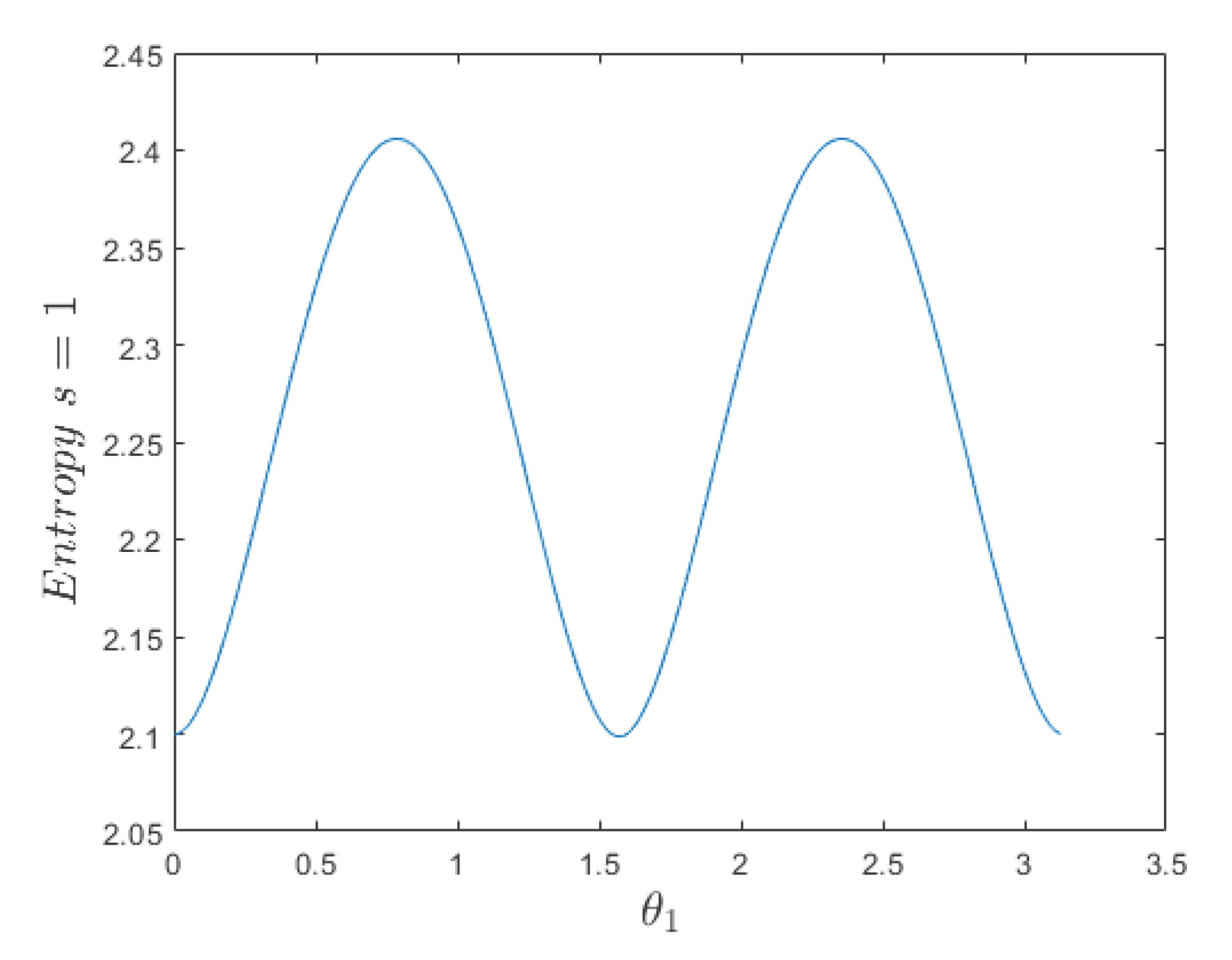
Figure 3.
Plot of Spin-Entropy of Entanglement (4) vs , a parameter that control the amount of entanglement. When there is no entanglement (product state), and when there is maximum entanglement. In all graphs the spin-entropy increases as the amount of entanglement increases.
Figure 3.
Plot of Spin-Entropy of Entanglement (4) vs , a parameter that control the amount of entanglement. When there is no entanglement (product state), and when there is maximum entanglement. In all graphs the spin-entropy increases as the amount of entanglement increases.
Disclaimer/Publisher’s Note: The statements, opinions and data contained in all publications are solely those of the individual author(s) and contributor(s) and not of MDPI and/or the editor(s). MDPI and/or the editor(s) disclaim responsibility for any injury to people or property resulting from any ideas, methods, instructions or products referred to in the content. |
© 2024 by the authors. Licensee MDPI, Basel, Switzerland. This article is an open access article distributed under the terms and conditions of the Creative Commons Attribution (CC BY) license (http://creativecommons.org/licenses/by/4.0/).
Copyright: This open access article is published under a Creative Commons CC BY 4.0 license, which permit the free download, distribution, and reuse, provided that the author and preprint are cited in any reuse.


