

Submitted:
20 March 2024
Posted:
26 March 2024
You are already at the latest version
Abstract
The Mann-Whitney effect is a measure for comparing survival distributions between two groups.
The Mann-Whitney effect is interpreted as the probability that a randomly selected subject in a
group survives longer than a randomly selected subject in the other group. Under the independence
assumption of two groups, the Mann-Whitney effect can be expressed as the traditional integral
formula of survival functions. However, when the survival times in two groups are not independent
each other, the traditional expression of the Mann-Whitney effect has to be modified. In this article,
we propose a copula-based approach to compute the Mann-Witney effect with parametric survival
models under dependence of two groups, which may arise in the potential outcome framework. In
addition, we develop a Shiny web app that can implement the proposed method via simple commands
(https://nkosuke.shinyapps.io/shiny_survival/). Through a simulation study, we show
the correctness of the proposed calculator. We apply the proposed methods to two real datasets.
Keywords:
censoring
; copula
; Hand’s paradox
; potential outcome
; Mann-Whitney effect
; stress-strength model
; two-sample comparison
; survival analysis
; survival function
; treatment effect
MSC: 62-04; 62D20; 62F10; 62N01; 62N03; 62N05
1. Introduction
When comparing the survival times of two independent groups, the Mann-Whitney parameter plays an important role in the two-sample problem ([1]). The Mann-Whitney parameter, say p, is defined as the probability that a random subject from one group (with survival time in group 1) survives longer than an independent random subject from the other group (with survival time in group 2), plus one-half the probability that the two subjects survive at the same time:
The Mann-Whitney effect relates to important statistical ideas, such as, the Mann-Whitney test ([2]), hazard ratios, and win ratio ([3]). The Mann-Whitney test examines the null hypothesis v.s. . The hazard ratio is the main effect measure of a Cox proportional hazards model, which is a typical statistical model in survival analysis. The win ratio w is given by the odds of p; that is, . That is, , or equivalently , implies a protective survival effect for group 1.
The problem of estimating the parameter p plays an important part in survival analysis. The basic idea was first studied by [4]. They illustrated an attractive relationship between the Mann-Whitney statistic and the stress-strength model. [1] first proposed a nonparametric estimator for p under independent censoring. Since then, this topic has been investigated by several researchers. In the following, we refer to some recent studies in the field of survival analysis. [5] modified Efron’s estimator for p under small sample sizes. [6] proposed a copula-graphic estimator for p and suggested the Mann-Whitney test to compare two survival distributions in the presence of dependent censoring. [7] introduced the Bayesian estimation of p for the log-Lindley distribution. [8] proposed estimating the Mann-Whitney effects in factorial clustered data. [9] developed methodologies for constructing fixed-accuracy confidence intervals of p when and follow geometric and the exponential distributions, respectively. [10] studied a estimation procedure of the stress-strength model for the two independent unit-half-normal distributions with different shape parameters. [11] investigated the effect of dependence of the valiables on p in the stress-strength model with the exponential margins. [12] proposed a group sequential method for estimating the Mann-Whitney parameter. [13] studied the estimator of p in point, interval, and Bayesian estimations when the stress valiables follow geometric and Lindley distribution. All the methods assumed that and are independent.
When and are independent of each other and continuous, one can estimate p with the marginal distributions based on the following integral:
That is, one can estimate p by estimating two marginal survival functions and . However, this is not the case when and are dependent; the phenomenon is sometimes called “Hand’s paradox” ([14]). This showed that the paradox arises when and are regarded as potential outcomes in the framework of causal inference. Therefore, p in the integral cannot be interpreted as the true treatment effect. Besides, dependence of outcomes from observation to observation is well-known in factorial designs and cross-over designs ([15]).
Since p is not identifiable solely from independently sampled data, [16] suggested a bound for p under all possible dependence structures for and . Alternatively, [17] reformulated p such that it can be identified from randomized treatment assignments. However, to estimate the true p, we must model the bivariate survival function of and . Copula is often used to model joint distributions of dependent survival times ([18,19]).
In this article, we propose a model for the bivariate survival function by using parametric copulas and parametric marginal distributions. We then derive a new formula for computing p by a one-dimensional integral. We also propose a new formula for p under the restricted follow-up. To make the proposed computation method for p to be easily performed by users, we develop a Shiny-based web app. Furthermore, we validate the accuracy of the proposed computation method and Shiny web app by simulations. We finally illustrate the proposed method by two real datasets.
The rest of the paper is organized as follows. In Section 2, we review copula-based models and introduce several well-known copula families. In this section, we show that one can compute p by Theorem in [20], and we extend the theorem to compute p when the follow-up time is restricted up to time . In Section 3, we introduce a Shiny web app in the R that can compute p via simple commands. In Section 4, we describe a simulation study to show the correctness of the proposed calculator for p. In Section 5, we illustrate a meaningful application of our proposed method using survival data.
2. Proposed Method
In this section, we first introduce copula-based bivariate survival models for and . We then propose our method for computing the Mann-Whitney effect p in Equation (1) under the copula models.
2.1. Copula Models for Dependent Survival Time
According to [21], any bivariate distribution function for can be formulated by using a copula. A bivariate copula is a bivariate distribution function for two uniform variables on ([22,23]). Let and be continuous survival times with marginal survival functions and , respectively. Initially, we model the bivariate survival function of and using a copula C:
This representation is useful since two marginal survival functions and are separated from the dependence structure C.
We will consider the following well-known families of bivariate copulas.
- The independence copula:
- The Clayton copula ([24]):
- The Gumbel copula ([25]):
- The Frank copula ([26]):
- The Farlie-Gumbel-Morgenstern (FGM) copula ([27]):
In Figure 1, we present scatterplots generated from various copulas with parameter . The Clayton copula (Figure 1 (b), (c)) shows lower tail dependence, the Gumbel copula (Figure 1 (d)) shows upper tail dependence, Frank copula (Figure 1 (e), (f)) shows symmetric dependence around the median, and the FGM copula (Figure 1 (g), (h)) is similar to the Frank copula. Unlike other copulas, the GB copula exhibits negative dependence only (Figure 1 (i)).
These copulas have been applied to survival data and other data analyses. The Clayton copula was applied to survival data with dependent censoring. For instance, [30] modeled dependence between survival and dependent censoring times in the survival data of tuberculosis cure. The Clayton, Gumbel, and Frank copula were also applied to dependently censored data in clinical trials or observational studies ([31,32,33]). The Gumbel, Frank, and FGM copulas were often used in competing risks models on survival data analysis ([34,35,36]). Copulas were also applied to multivariate meta-analysis; [37] and [38] proposed a bivariate Clayton, FGM and Gumbel models for bivariate meta-analysis. The Gumbel-Barnett copula has the simple form and is suitable for modeling negative dependence ([22,28]). Therefore, it is important to consider a variety of copulas for dependent survival times.
To see the strength of dependence in a copula, can be transformed to Kendall’s tau, . Kendall’s tau is a well-known measure to assess the dependence between two variables. Under the copula model (2), Kendall’s tau for and is expressed as
Kendall’s does not depend on the marginals, and is solely determined by the copula. Therefore, it is advantageous over the Pearson correlation for and . Kendall’s of each copula is expressed as follow.
- The independence copula:
- The Clayton copula:
- The Gumbel copula:
- The Frank copula:
- The FGM copula:
- The GB copula:
2.2. Proposed Method for Computing p
In this section, we propose a new formula for computing p under the survival copula model (2). Let and . For computing p, we will use the conditional distribution function for U given , which is the partial derivative of C with respect to v:
Then, by slightly modifying Theorem of [20], p can be expressed as the univariate integral on :
We note that Theorem of [20] is not directly applicable to the survival copula model (2) since that theorem is designed for the copula model .
Equation (3) with aforementioned copulas is computed by the following formulas:
- The Clayton copula
- The Gumbel copula
- The Frank copula
- The FGM copula
- The GB copula
In order to compute p by the above formulas, we need to specify , , and . One can specify and by continuous parametric models that will be discussed in Section 2.4. One can try different values for in a sensitivity analysis. Note that the above calculations are not applicable for discrete parametric models for and .
2.3. Computing p with Follow-Up Time
For survival data, the follow-up period is often limitted. When a subject survives longer than the follow-up period, one may treat the survival time of the subject as equal to the follow-up period ([5,39,40]). In this section, we assume that every subject has a common follow-up time . This means that we define the Mann-Whitney effect for and . We now obtain p with follow-up time from the following theorem, a straightforward expansion of Theorem in [20].
Theorem 1.
The Mann-Whitney effect p with a follow-up time τ is written as the univariate integral:
Equation 4 with different copulas is computed by the following formulas:
- The Clayton copula
- The Gumbel copula
- The Frank copula
- The FGM copula
- The GB copula
2.4. Marginal Survival Distributions
To compute p and , we considered following three parametric distributions as the marginal survival distributions of group :
- The exponential distribution:where is a rate parameter.
- The Weibull distribution:where is a scale parameter and is a shape parameter.
- The gamma distribution:where is a scale parameter and is a shape parameter, and is the gamma function, and is the lower incomplete gamma function. The gamma distribution has no simple closed-form expression for the inverse survival function. Therefore, one can use approximations for the inverse survival function. In Section 3, we use the R function “qgamma” to calculate the quantile funciton of the gamma distribution.
In Figure 2, we present survival curves of three parametric distributions, the exponential, Weibull, and gamma distributions with different parameters. These plots show that these distributions can represent almost any continuous survival curve that will be encountered in practice.
Example 1.
Let the marginals be the exponential distributions with parameter and and are independent. Then by Theorem 1 with , p is given by
□
Example 2.
Let the marginals be the exponential distributions with parameter and be the Clayton copula with parameter . Then Kendall’s τ is given by
and by Theorem 1 with , p is given by
When , is given by
When , . Here, we computed the last two equations by a numerical integration by the R function "integrate". □
Parameters for the marginal distributions can be estimated by maximum likelihood estimators (MLEs) when the survival data are available in two groups (Section 5).
3. Software and Web App
We developed a Shiny-based web app to implement the proposed method of computing p. The Shiny app is available at (https://nkosuke.shinyapps.io/shiny_survival/) and can be used by any environment, including smartphones. Using this web app, users can choose a marginal survival distribution, copula, and the relevant parameters to compute p. Our web app is easy to use without knowledge of the R.
3.1. Input
We considered three marginal survival distributions; the exponential, Weibull, and gamma distributions. We considered the Clayton, Gumbel, Frank, FGM, and GB copulas. One can choose marginal distributions and copulas, set their parameters, and choose the langage displayed on the screen in the input panels on the left-hand of our app (Figure 3). Furthermore, one can set a follow-up time with a slider bar. In Figure 3, we set the marginal survival distribution = “Exponential Distribution”, , , , copula = “Clayton”, and the langage displayed on the screen “English”.
3.2. Output
This app displays several formulas, survival curves of each group, p, , and Kendall’s . These formulas include marginal and bivariate survival functions and formulas of p and based on the input values. The theoretical values of p and are displayed together with survival curves.
Figure 3 displays the web app. In this settings, we have the output , Kendall’s .
4. Simulation Studies
To show the correctness of the proposed calculator for p, we conduced a simulation study. For the simulation study, we set the marginal survival functions to be the exponential distributions with , the Weibull distributions with , and the gamma distributions with . Furthermore, we set the copula parameters, the Clayton copula with , the Gumbel copula with , the Frank copula with , the FGM copula with , the GB copula with , and follow-up time . We generated 100,000 pairs , from the bivariate survival function based on the aforementioned settings, and calculated the Monte Carlo simulation values defined as,
Table 1 shows that the simulation values are nearly equal to the theoretical values computed by the formula of Theorem 1 for every setting. In conclusion, our simulations show that Theorem 1 is correct, and the Shiny web app based on Theorem 1 is reliable.
5. Numerical Examples
In this section, we apply our proposed methods to a tongue cancer dataset and a prostate cancer dataset. Before analyzing the real datasets, we introduce basic notations and ideas for estimating p by using censored data. Let be survival times, be censored times, be observed time, and be event indicator. What we observe is and . That is, is 0 or 1 according to whether is a censored time or a survival time. As the exponential distribution is shown to fit well for and , we obtained MLE of the exponential hazard rate by
Then, by applying the values of the MLE to the proposed Shiny web app, we obtained the estimators and , where was chosen appropriately (Section 5.1 and Section 5.2). On the other hand, under the independence assumption of and , the naïve estimator of p is
where and is a Kaplan-Meier (KM) estimator. However, this estimate is subject to the independence of two groups. Therefore, the proposed estimator is useful to examine the sensitivity under a variety of dependence structures via copulas.
5.1. Tongue Cancer Data
The tongue dataset is available in the R package KMsurv. It has 80 observations and contains: type (Tumor DNA profile: 1 = aneuploid tumor, 2 = diploid tumor), time (Time to death or on-study time (weeks)), and death (Event indicator: 0 = alive, 1 = dead). It contains observations in aneuploid cancer group (), and observations in diploid cancer group (). We considered the follow-up time and obtained . The tongue cancer data resulted in and . In Figure 4, the KM estimators of each groups and the estimated exponential survival curves are plotted. We conducted sensitivity analyses using copula-based approach. We calculated by Theorem 1 under weak, strong positive, and negative independences. We calculated via the web app (Section 3). Figure 5 shows the output under the independent, Clayton, Gumbel, Frank, FGM, and GB copula with parameter . The results under all copulas are summarized in Table 2. We obtained the ranged from to and concluded that a subject in DNA-aneuploid tumor gruop survives longer than in DNA-diploid tumor group. This conclusion did not change under any depencence structures we conducted.
5.2. Prostate Cancer Data
The prostate cancer data is avalible in the R package asaur ([41]). It has 14,294 observations and contains: grade (moderately differentiated and poorly differentiated), survTime (time from diagnosis to death or last date known alive), and status (Event indicator: 0 = censored, 1 = death from prostate cancer). It contains observations in moderately differentiated group (), and observations in poorly differentiated group ().
The prostate cancer data resulted in , , and . In Figure 6, we plot the KM estimators of each group and estimated exponential survival curves. We calculated by Theorem 1 with copulas and several parameters. We calculated under the independent, Clayton, Gumbel, Frank, FGM, and GB copulas with parameter via the web app (Figure 7). The results for all scenarios are summarized in Table 3. We obtained the ranged from to and concluded that a subject in moderately differentiated gruop survives longer than in poorly differentiated group. The range of is narrower than one of tongue cancer dataset. The results may be caused by the distinct difference of survival curves between two groups, the short follow-up time for two groups and large sample size.
6. Conclusion
The Mann-Whitney effect has been widely used for survival analysis, which can provide the meaningful measure for treatment effects for survival outcomes. However, the Mann-Whitney effect may not be interpreted as the true treatment effect under dependence of two survival times. In this article, we proposed a parametric copula-based approach for estimating the Mann-Witney effect p under depencence structures for two survival times. We derived the formulas of p under a variety of copulas and marginal survival functions. We also introduced a web-based calculator for p for users. Simulation studies demonstrated the correctness of the proposed calculator for p under a variety of the parametric marginal survival distributions and copulas. The results of data analyses show that the proposed method gives possible changes of p under various denpendence and enables to examine the sensitivity.
In the examples of real datasets, we obtained under the Clayton, Gumbel, Frank, FGM, GB copulas with varying parameters. The value of ranged from to in tongue cancer dataset, from to in prostate cancer dataset. We obtained the narrow ranges whose lower bound did not include the null value of . The result is consistent with previous studies that Hand’s paradox does not occur under strictly monotonic effect ([14,42]). While more complex dependence structures with various copulas might be considered, the conclusion may not change much.
The main limitation of the present article is that we only discussed the “parametric” approach. However, in practice, researchers may use the “semi-” or “non-parametric” approach. In future work, we will examine the method of computing p without parametric assumptions. Another extension is to include covariates or secondary outcomes in the model, which help obtain narrow bounds for treatment effects ([43]). Another limitation is that only one-parameter copulas are implemented. There are multi-parameter copulas that deserve attention ([22,28,44]).
Funding
This research was funded by [JSPS KAKENHI] grant number [22K11948] and grant number [20H04147].
References
- Efron, B. The two sample problem with censored data. Proceedings of the fifth Berkeley symposium on mathematical statistics and probability, 1967, Vol. 4, pp. 831–853.
- Mann, H.B.; Whitney, D.R. On a test of whether one of two random variables is stochastically larger than the other. Ann. Math. Statistics 1947, 18, 50–60. [Google Scholar] [CrossRef]
- Pocock, S.J.; Ariti, C.A.; Collier, T.J.; Wang, D. The win ratio: a new approach to the analysis of composite endpoints in clinical trials based on clinical priorities. European Heart Journal 2011, 33, 176–182. [Google Scholar] [CrossRef] [PubMed]
- Birnbaum, Z.W. On a use of the Mann-Whitney statistic. Proceedings of the Third Berkeley Symposium on Mathematical Statistics and Probability, 1954–1955, vol. I. Univ. California Press, Berkeley-Los Angeles, Calif., 1956, pp. 13–17.
- Dobler, D.; Pauly, M. Bootstrap- and permutation-based inference for the Mann-Whitney effect for right-censored and tied data. TEST 2018, 27, 639–658. [Google Scholar] [CrossRef]
- Emura, T.; Hsu, J.H. Estimation of the Mann-Whitney effect in the two-sample problem under dependent censoring. Comput. Statist. Data Anal. 2020, 150, 106990–17. [Google Scholar] [CrossRef]
- Biswas, A.; Chakraborty, S.; Mukherjee, M. On estimation of stress-strength reliability with log-Lindley distribution. J. Stat. Comput. Simul. 2021, 91, 128–150. [Google Scholar] [CrossRef]
- Rubarth, K.; Sattler, P.; Zimmermann, H.G.; Konietschke, F. Estimation and Testing of Wilcoxon-Mann-Whitney Effects in Factorial Clustered Data Designs. Symmetry 2022, 14. https://www.mdpi.com/2073-8994/14/2/244. [Google Scholar] [CrossRef]
- Hu, J.; Zhuang, Y.; Goldiner, C. Fixed-accuracy confidence interval estimation of P(X<Y) under a geometric-exponential model. Jpn. J. Stat. Data Sci. 2021, 4, 1079–1104. [Google Scholar] [CrossRef]
- de la Cruz, R.; Salinas, H.S.; Meza, C. Reliability Estimation for Stress-Strength Model Based on Unit-Half-Normal Distribution. Symmetry 2022, 14. https://www.mdpi.com/2073-8994/14/4/837. [Google Scholar] [CrossRef]
- Patil, D.; Naik-Nimbalkar, U.V.; Kale, M.M. Effect of Dependency on the Estimation of P[Y>X] in Exponential Stress-strength Models. Austrian Journal of Statistics 2022, 51, 10–34, https://www.ajs.or.at/index.php/ajs/article/view/1293. [Google Scholar] [CrossRef]
- Nowak, C.P.; Mütze, T.; Konietschke, F. Group sequential methods for the Mann-Whitney parameter. Stat. Methods Med. Res. 2022, 31, 2004–2020. [Google Scholar] [CrossRef]
- Singh, B.; Nayal, A.S.; Tyagi, A. Estimation of P [Y< Z] under Geometric-Lindley model. Ricerche di Matematica, 2023; 1–32. [Google Scholar]
- Hand, D.J. On Comparing Two Treatments. The American Statistician 1992, 46, 190–192. [Google Scholar] [CrossRef]
- Cochran, W.G.; Cox, G.M. Experimental designs; John Wiley & Sons, Inc., New York; Chapman & Hall, Ltd., London, 1957; pp. xiv+617. 2nd ed.
- Fan, Y.; Park, S.S. Sharp bounds on the distribution of treatment effects and their statistical inference. Econometric Theory 2010, 26, 931–951. [Google Scholar] [CrossRef]
- Fay, M.P.; Brittain, E.H.; Shih, J.H.; Follmann, D.A.; Gabriel, E.E. Causal estimands and confidence intervals associated with Wilcoxon-Mann-Whitney tests in randomized experiments. Stat. Med. 2018, 37, 2923–2937. [Google Scholar] [CrossRef] [PubMed]
- Emura, T.; Matsui, S.; Rondeau, V. Survival analysis with correlated endpoints; SpringerBriefs in Statistics, Springer, Singapore, 2019; pp. xvii+118. [CrossRef]
- Li, D.; Hu, X.J.; Wang, R. Evaluating association between two event times with observations subject to informative censoring. J. Amer. Statist. Assoc. 2023, 118, 1282–1294. [Google Scholar] [CrossRef] [PubMed]
- Emura, T.; Pan, C.H. Parametric likelihood inference and goodness-of-fit for dependently left-truncated data, a copula-based approach. Statist. Papers 2020, 61, 479–501. [Google Scholar] [CrossRef]
- Sklar, M. Fonctions de répartition à n dimensions et leurs marges. Publ. Inst. Statist. Univ. Paris 1959, 8, 229–231. [Google Scholar]
- Nelsen, R.B. An introduction to copulas, second ed.; Springer Series in Statistics, Springer, New York, 2006; pp. xiv+269. [CrossRef]
- Geenens, G. (Re-)Reading Sklar (1959);A Personal View on Sklar’s Theorem. Mathematics 2024, 12. https://www.mdpi.com/2227-7390/12/3/380. [Google Scholar] [CrossRef]
- Clayton, D.G. A model for association in bivariate life tables and its application in epidemiological studies of familial tendency in chronic disease incidence. Biometrika 1978, 65, 141–151. [Google Scholar] [CrossRef]
- Gumbel, E.J. Distributions des valeurs extrêmes en plusieurs dimensions. Publ. Inst. Statist. Univ. Paris 1960, 9, 171–173. [Google Scholar]
- Frank, M.J. On the simultaneous associativity of F(x,y) and x+y-F(x,y). Aequationes Math. 1979, 19, 194–226. [Google Scholar] [CrossRef]
- Morgenstern, D. Einfache Beispiele zweidimensionaler Verteilungen. Mitteilungsbl. Math. Statist. 1956, 8, 234–235. [Google Scholar]
- Chesneau, C. On the Gumbel-Barnett extended Celebioglu-Cuadras copula. Jpn. J. Stat. Data Sci. 2023, 6, 759–781. [Google Scholar] [CrossRef]
- Toparkus, A.M.; Weißbach, R. Testing Truncation Dependence: The Gumbel-Barnett Copula. 2024; arXiv:stat.ME/2305.19675. [Google Scholar] [CrossRef]
- Schneider, S.; dos Reis, R.C.P.; Gottselig, M.M.F.; Fisch, P.; Knauth, D.R.; Vigo, A. Clayton copula for survival data with dependent censoring: an application to a tuberculosis treatment adherence data. Stat. Med. 2023, 42, 4057–4081. [Google Scholar] [CrossRef]
- Sun, T.; Ding, Y. Copula-based semiparametric regression method for bivariate data under general interval censoring. Biostatistics 2021, 22, 315–330. [Google Scholar] [CrossRef] [PubMed]
- Moradian, H.; Larocque, D.; Bellavance, F. Survival forests for data with dependent censoring. Stat. Methods Med. Res. 2019, 28, 445–461. [Google Scholar] [CrossRef] [PubMed]
- Farzana, W.; Basree, M.M.; Diawara, N.; Shboul, Z.A.; Dubey, S.; Lockhart, M.M.; Hamza, M.; Palmer, J.D.; Iftekharuddin, K.M. Prediction of Rapid Early Progression and Survival Risk with Pre-Radiation MRI in WHO Grade 4 Glioma Patients. Cancers 2023, 15. https://www.mdpi.com/2072-6694/15/18/4636. [Google Scholar] [CrossRef]
- Escarela, G.; Carrière, J.F. Fitting competing risks with an assumed copula. Stat. Methods Med. Res. 2003, 12, 333–349. [Google Scholar] [CrossRef]
- Chen, Y.H. Semiparametric marginal regression analysis for dependent competing risks under an assumed copula. J. R. Stat. Soc. Ser. B Stat. Methodol. 2010, 72, 235–251. [Google Scholar] [CrossRef]
- Shih, J.H.; Emura, T. Likelihood-based inference for bivariate latent failure time models with competing risks under the generalized FGM copula. Comput. Statist. 2018, 33, 1293–1323. [Google Scholar] [CrossRef]
- Shih, J.H.; Konno, Y.; Chang, Y.T.; Emura, T. Estimation of a common mean vector in bivariate meta-analysis under the FGM copula. Statistics 2019, 53, 673–695. [Google Scholar] [CrossRef]
- Shih, J.H.; Konno, Y.; Chang, Y.T.; Emura, T. Copula-Based Estimation Methods for a Common Mean Vector for Bivariate Meta-Analyses. Symmetry 2022, 14. https://www.mdpi.com/2073-8994/14/2/186. [Google Scholar] [CrossRef]
- Dobler, D.; Pauly, M. Factorial analyses of treatment effects under independent right-censoring. Stat. Methods Med. Res. 2020, 29, 325–343. [Google Scholar] [CrossRef] [PubMed]
- Emura, T.; Ditzhaus, M.; Dobler, D.; Murotani, K. Factorial survival analysis for treatment effects under dependent censoring. Stat. Methods Med. Res. 2024, 33, 61–79. [Google Scholar] [CrossRef] [PubMed]
- Moore, D.F. Applied survival analysis using R; Vol. 473, Springer, 2016.
- Greenland, S.; Fay, M.P.; Brittain, E.H.; Shih, J.H.; Follmann, D.A.; Gabriel, E.E.; Robins, J.M. On causal inferences for personalized medicine: how hidden causal assumptions led to erroneous causal claims about the D-value. Amer. Statist. 2020, 74, 243–248. [Google Scholar] [CrossRef]
- Yin, Y.; Cai, Z.; Zhou, X.H. Using secondary outcome to sharpen bounds for treatment harm rate in characterizing heterogeneity. Biom. J. 2018, 60, 879–892. [Google Scholar] [CrossRef]
- SUSAM, S.O. A multi-parameter Generalized Farlie-Gumbel-Morgenstern bivariate copula family via Bernstein polynomial. Hacettepe Journal of Mathematics and Statistics 2022, 51, 618–631. [Google Scholar] [CrossRef]
Figure 1.
Scatter plots of 3,000 data points generated from the copula distribution with parameter .
Figure 1.
Scatter plots of 3,000 data points generated from the copula distribution with parameter .
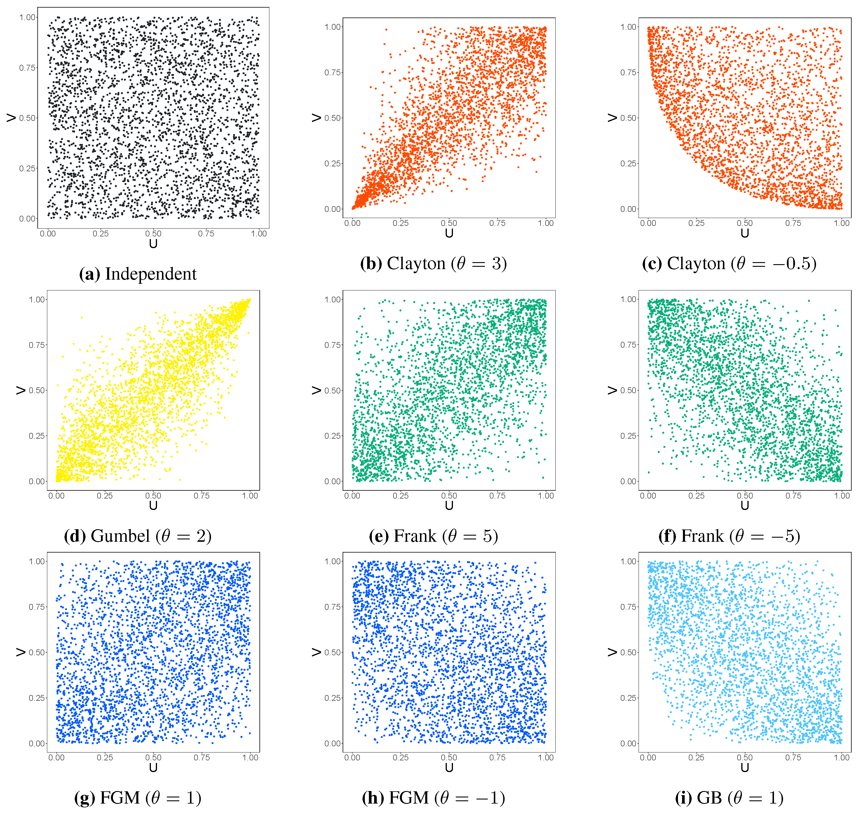
Figure 2.
Survival-curve plots of the parametric distribution functions.
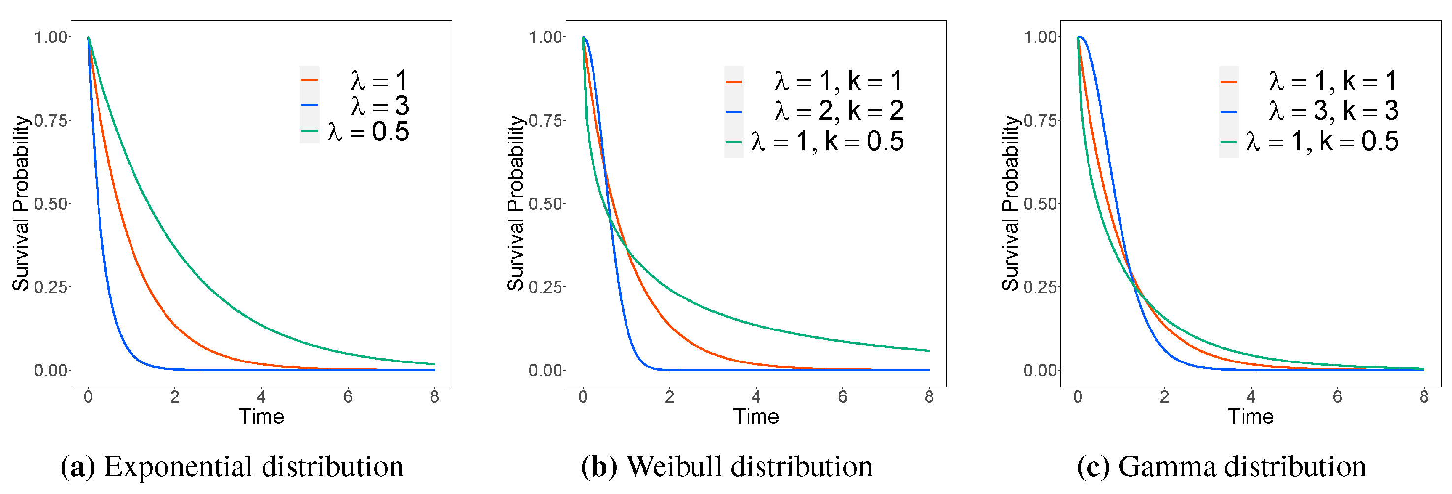
Figure 3.
The web app showing the results for computing p and .
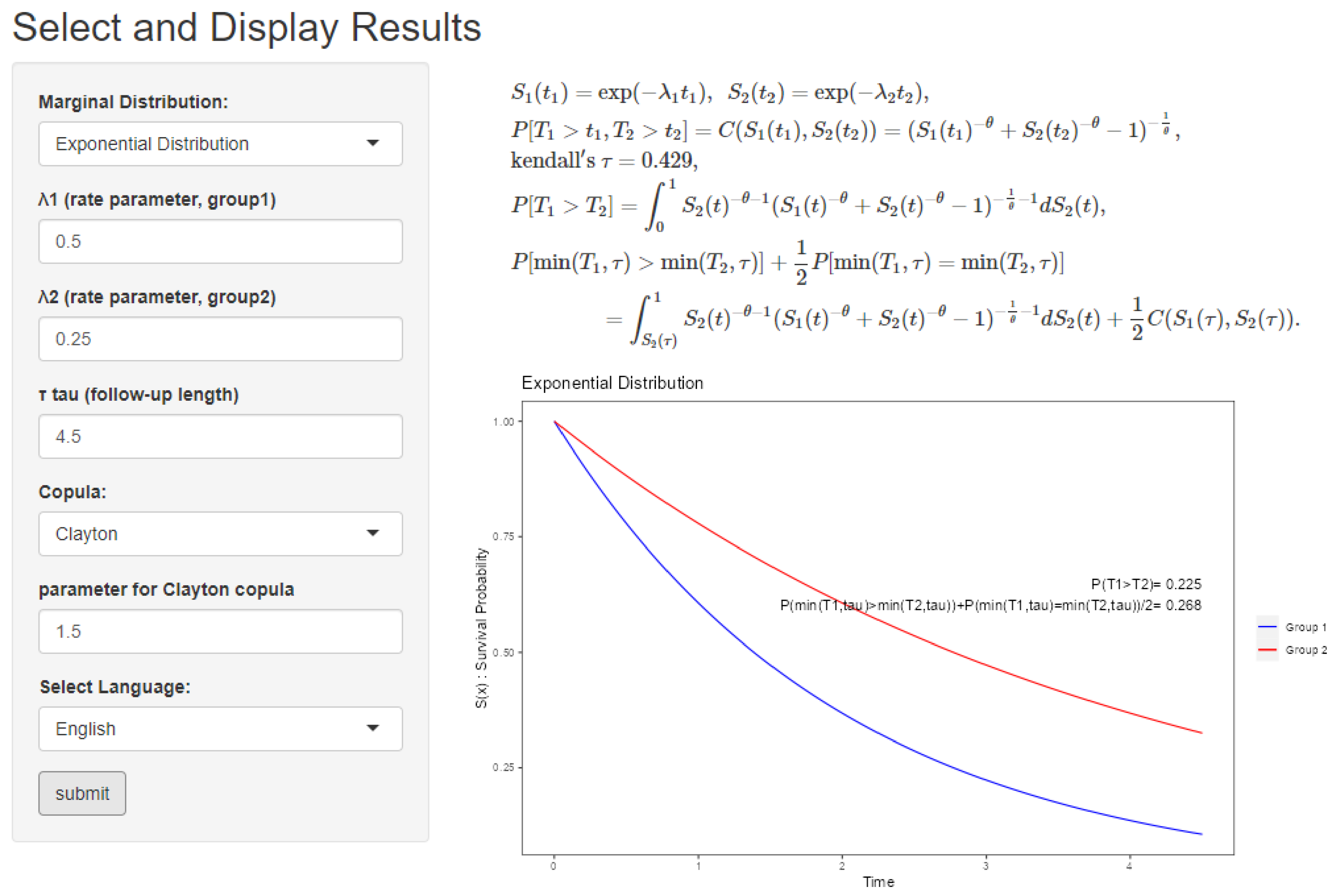
Figure 4.
KM estimators for DNA-aneuploid tumor and DNA-diploid tumor group and exponential survival curves with MLE of exponential hazard rates, .
Figure 4.
KM estimators for DNA-aneuploid tumor and DNA-diploid tumor group and exponential survival curves with MLE of exponential hazard rates, .
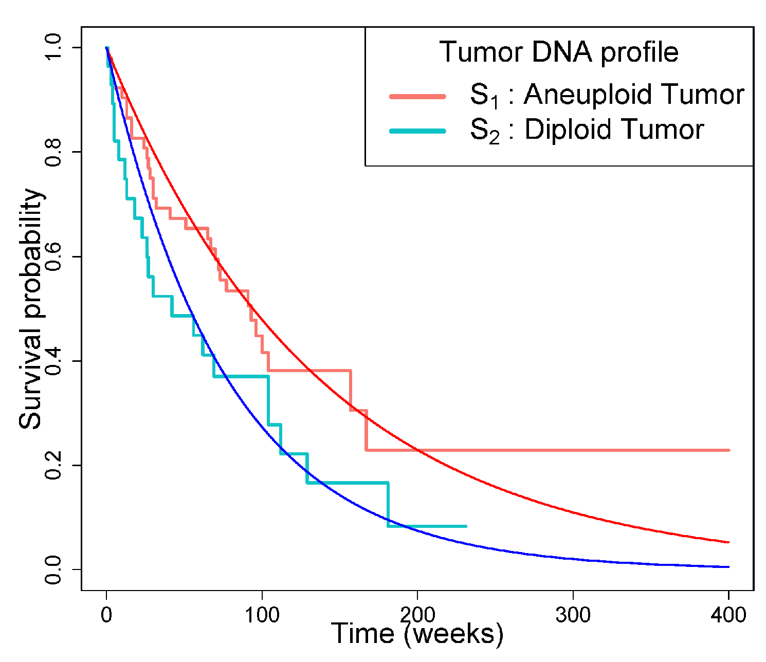
Figure 5.
Example for the tongue cancer dataset on the web app. This setting is marginal distribution: “Exponential”, , copula: “Clayton”, copula parameter: , and langage: “English”.
Figure 5.
Example for the tongue cancer dataset on the web app. This setting is marginal distribution: “Exponential”, , copula: “Clayton”, copula parameter: , and langage: “English”.
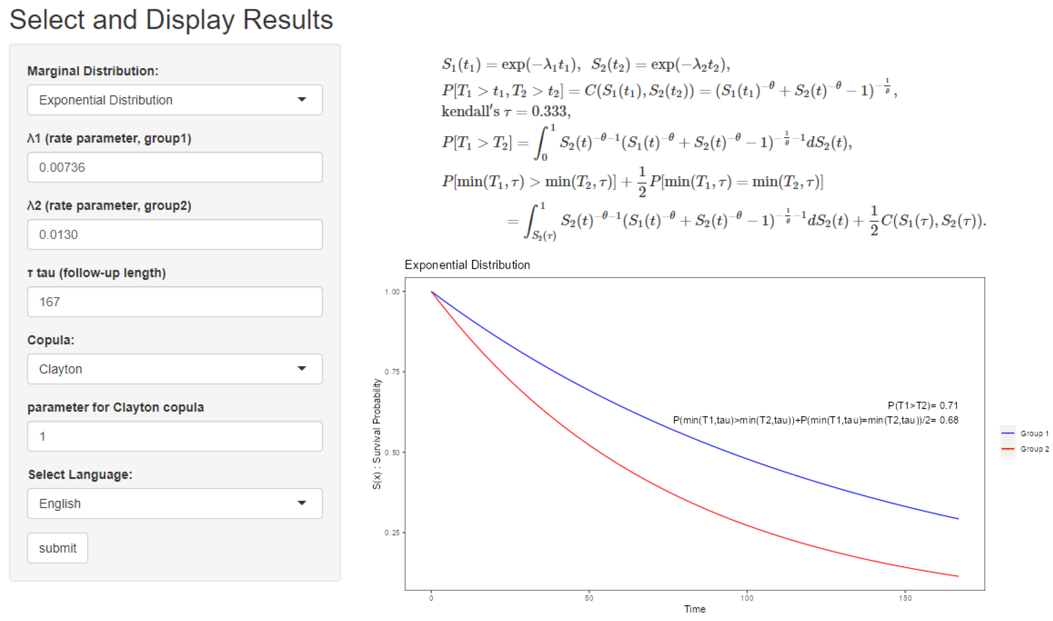
Figure 6.
KM estimators for mode grade and poor grade group and exponential survival curves with MLE of exponential hazard rates, .
Figure 6.
KM estimators for mode grade and poor grade group and exponential survival curves with MLE of exponential hazard rates, .
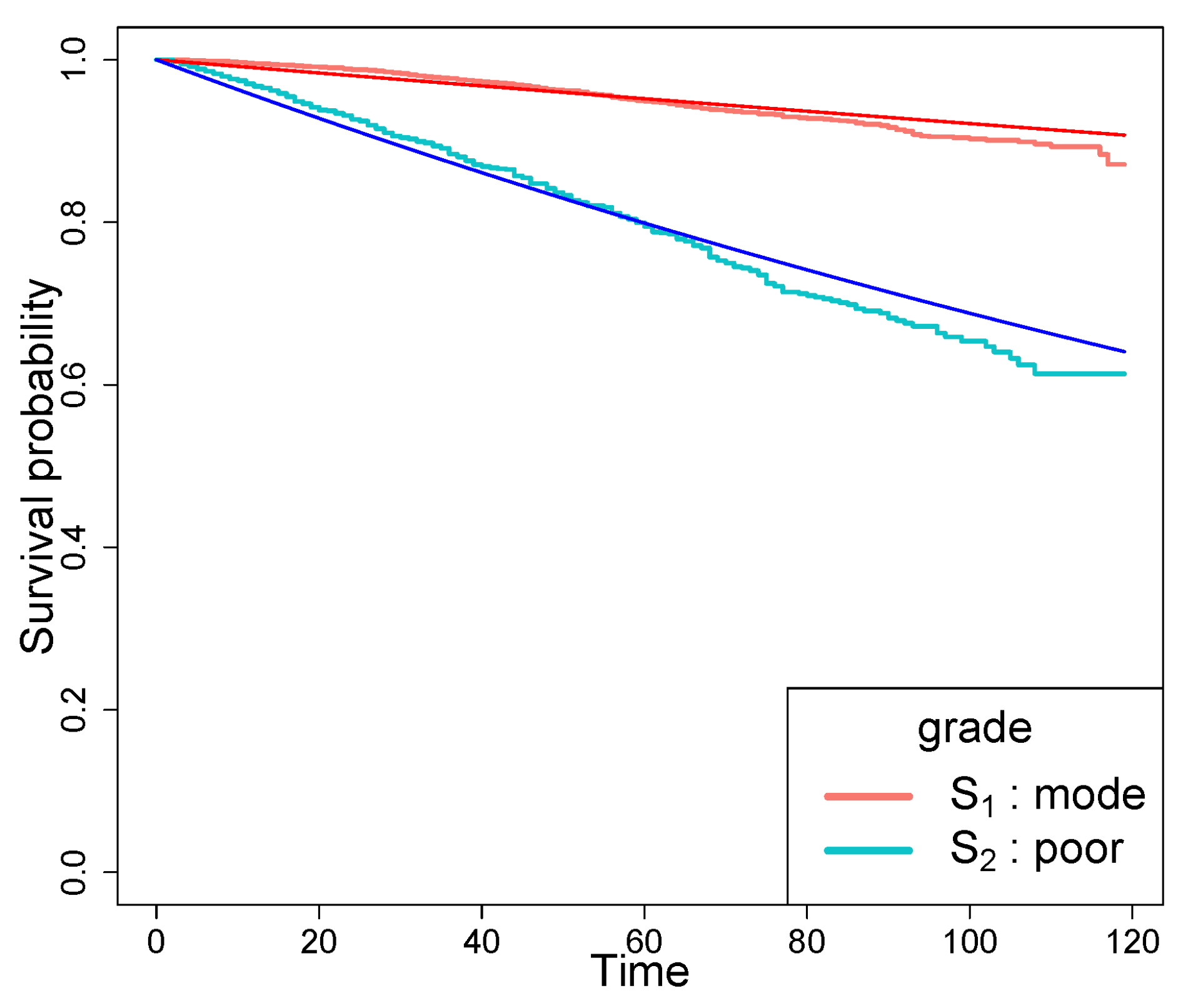
Figure 7.
Example for the tongue cancer dataset on the web app. This setting is marginal distribution: “Exponential”, , copula: “Gumbel”, copula parameter: , and langage: “English”.
Figure 7.
Example for the tongue cancer dataset on the web app. This setting is marginal distribution: “Exponential”, , copula: “Gumbel”, copula parameter: , and langage: “English”.
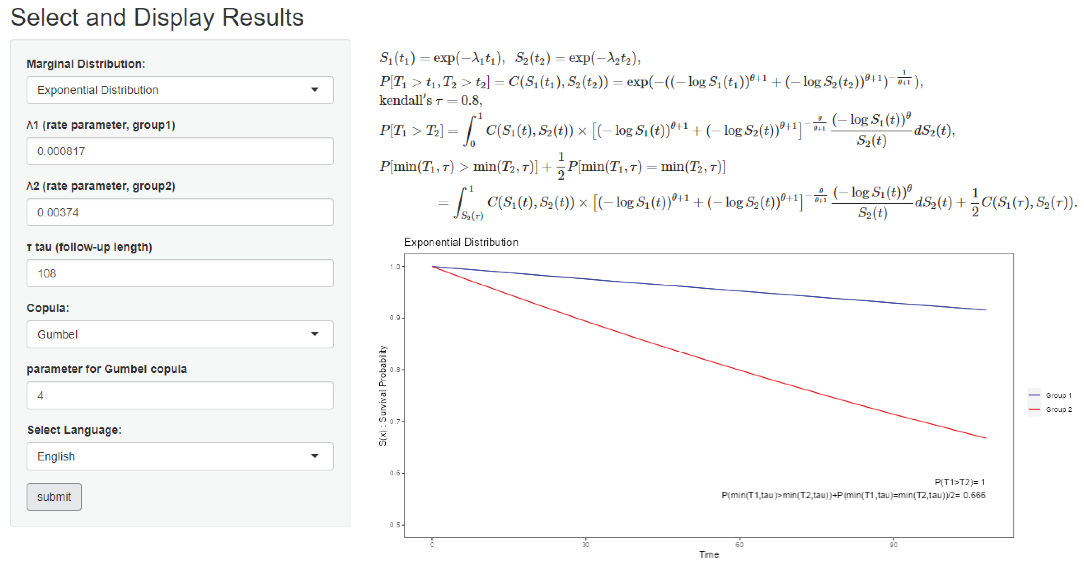

Table 1.
Comparison of the theoretical value and the simulation value for calculating defined in Theorem 1.
Table 1.
Comparison of the theoretical value and the simulation value for calculating defined in Theorem 1.
| Distribution | Copula | ||||||||||||
| Exponential | Clayton | 1 | 0.33 | 1 | - | 2 | - | 0.645 | 0.643 | 0.737 | 0.738 | 0.744 | 0.746 |
| 5 | 0.71 | 1 | - | 2 | - | 0.704 | 0.706 | 0.872 | 0.872 | 0.881 | 0.883 | ||
| 10 | 0.83 | 1 | - | 2 | - | 0.746 | 0.745 | 0.920 | 0.921 | 0.930 | 0.930 | ||
| Gumbel | 0 | 0.00 | 1 | - | 2 | - | 0.629 | 0.631 | 0.666 | 0.666 | 0.666 | 0.665 | |
| 4 | 0.80 | 1 | - | 2 | - | 0.798 | 0.799 | 0.961 | 0.961 | 0.970 | 0.969 | ||
| Frank | -5 | -0.46 | 1 | - | 2 | - | 0.615 | 0.615 | 0.622 | 0.622 | 0.622 | 0.622 | |
| 1 | 0.11 | 1 | - | 2 | - | 0.636 | 0.636 | 0.684 | 0.684 | 0.685 | 0.685 | ||
| 5 | 0.46 | 1 | - | 2 | - | 0.674 | 0.674 | 0.771 | 0.768 | 0.773 | 0.772 | ||
| FGM | -1 | -0.22 | 1 | - | 2 | - | 0.617 | 0.617 | 0.633 | 0.634 | 0.633 | 0.631 | |
| 0 | 0.00 | 1 | - | 2 | - | 0.629 | 0.629 | 0.666 | 0.666 | 0.666 | 0.666 | ||
| 1 | 0.22 | 1 | - | 2 | - | 0.642 | 0.641 | 0.699 | 0.697 | 0.700 | 0.702 | ||
| GB | 0.5 | -0.21 | 1 | - | 2 | - | 0.623 | 0.624 | 0.642 | 0.643 | 0.642 | 0.641 | |
| 1 | -0.36 | 1 | - | 2 | - | 0.617 | 0.616 | 0.629 | 0.628 | 0.629 | 0.632 | ||
| Weibull | Clayton | 1 | 0.33 | 1 | 0.5 | 2 | 1 | 0.497 | 0.496 | 0.594 | 0.589 | 0.603 | 0.602 |
| 5 | 0.71 | 1 | 0.5 | 2 | 1 | 0.482 | 0.480 | 0.644 | 0.645 | 0.653 | 0.654 | ||
| 10 | 0.83 | 1 | 0.5 | 2 | 1 | 0.472 | 0.472 | 0.645 | 0.645 | 0.654 | 0.653 | ||
| Gumbel | 0 | 0.00 | 1 | 0.5 | 2 | 1 | 0.511 | 0.509 | 0.560 | 0.562 | 0.562 | 0.562 | |
| 4 | 0.80 | 1 | 0.5 | 2 | 1 | 0.425 | 0.424 | 0.584 | 0.585 | 0.593 | 0.594 | ||
| Frank | -5 | -0.46 | 1 | 0.5 | 2 | 1 | 0.528 | 0.530 | 0.542 | 0.541 | 0.542 | 0.543 | |
| 1 | 0.11 | 1 | 0.5 | 2 | 1 | 0.505 | 0.504 | 0.566 | 0.565 | 0.569 | 0.572 | ||
| 5 | 0.46 | 1 | 0.5 | 2 | 1 | 0.486 | 0.486 | 0.592 | 0.595 | 0.597 | 0.597 | ||
| FGM | -1 | -0.22 | 1 | 0.5 | 2 | 1 | 0.521 | 0.523 | 0.548 | 0.549 | 0.549 | 0.551 | |
| 0 | 0.00 | 1 | 0.5 | 2 | 1 | 0.511 | 0.509 | 0.560 | 0.563 | 0.562 | 0.562 | ||
| 1 | 0.22 | 1 | 0.5 | 2 | 1 | 0.501 | 0.503 | 0.572 | 0.574 | 0.575 | 0.577 | ||
| GB | 0.5 | -0.21 | 1 | 0.5 | 2 | 1 | 0.519 | 0.520 | 0.549 | 0.546 | 0.549 | 0.548 | |
| 1 | -0.36 | 1 | 0.5 | 2 | 1 | 0.526 | 0.526 | 0.545 | 0.545 | 0.545 | 0.545 | ||
| Gamma | Clayton | 1 | 0.33 | 1 | 1.5 | 2 | 2 | 0.529 | 0.529 | 0.651 | 0.649 | 0.679 | 0.678 |
| 5 | 0.71 | 1 | 1.5 | 2 | 2 | 0.530 | 0.528 | 0.763 | 0.763 | 0.809 | 0.810 | ||
| 10 | 0.83 | 1 | 1.5 | 2 | 2 | 0.534 | 0.533 | 0.817 | 0.816 | 0.862 | 0.863 | ||
| Gumbel | 0 | 0.00 | 1 | 1.5 | 2 | 2 | 0.530 | 0.530 | 0.611 | 0.612 | 0.615 | 0.614 | |
| 4 | 0.80 | 1 | 1.5 | 2 | 2 | 0.545 | 0.546 | 0.813 | 0.813 | 0.853 | 0.853 | ||
| Frank | -5 | -0.46 | 1 | 1.5 | 2 | 2 | 0.532 | 0.530 | 0.584 | 0.584 | 0.584 | 0.583 | |
| 1 | 0.11 | 1 | 1.5 | 2 | 2 | 0.530 | 0.529 | 0.622 | 0.622 | 0.628 | 0.628 | ||
| 5 | 0.46 | 1 | 1.5 | 2 | 2 | 0.530 | 0.530 | 0.679 | 0.679 | 0.694 | 0.692 | ||
| FGM | -1 | -0.22 | 1 | 1.5 | 2 | 2 | 0.531 | 0.533 | 0.591 | 0.591 | 0.592 | 0.591 | |
| 0 | 0.00 | 1 | 1.5 | 2 | 2 | 0.530 | 0.529 | 0.611 | 0.610 | 0.615 | 0.614 | ||
| 1 | 0.22 | 1 | 1.5 | 2 | 2 | 0.529 | 0.529 | 0.631 | 0.631 | 0.639 | 0.640 | ||
| GB | 0.5 | -0.21 | 1 | 1.5 | 2 | 2 | 0.531 | 0.532 | 0.597 | 0.598 | 0.598 | 0.598 | |
| 1 | -0.36 | 1 | 1.5 | 2 | 2 | 0.532 | 0.532 | 0.589 | 0.592 | 0.590 | 0.588 | ||
Table 2.
Estimates for fitting the KM estimator (independent) and with the exponential marginal survival distributions (the independent, Clayton, Gumbel, Frank, FGM, GB copulas) for the tongue cancer dataset.
Table 2.
Estimates for fitting the KM estimator (independent) and with the exponential marginal survival distributions (the independent, Clayton, Gumbel, Frank, FGM, GB copulas) for the tongue cancer dataset.
| Copula | marginal distribution | |||
|---|---|---|---|---|
| Independent | KM estimator | - | - | 0.632 |
| Independent | exponential | - | 0.638 | 0.633 |
| Clayton | exponential | 1 | 0.709 | 0.676 |
| 5 | 0.856 | 0.799 | ||
| Gumbel | exponential | 4 | 0.906 | 0.862 |
| Frank | exponential | -5 | 0.600 | 0.600 |
| 5 | 0.733 | 0.714 | ||
| FGM | exponential | -1 | 0.609 | 0.609 |
| 1 | 0.666 | 0.658 | ||
| GB | exponential | 0.5 | 0.617 | 0.617 |
| 1 | 0.606 | 0.606 |
Table 3.
Estimates for fitting the KM estimator (independent) and with the exponential marginal survival distributions (the independent, Clayton, Gumbel, Frank, FGM, GB copulas) for the prostate cancer dataset.
Table 3.
Estimates for fitting the KM estimator (independent) and with the exponential marginal survival distributions (the independent, Clayton, Gumbel, Frank, FGM, GB copulas) for the prostate cancer dataset.
| Copula | marginal distribution | |||
|---|---|---|---|---|
| Independent | KM estimator | - | - | 0.679 |
| Independent | exponential | - | 0.821 | 0.625 |
| Clayton | exponential | 1 | 0.889 | 0.626 |
| 5 | 0.958 | 0.635 | ||
| Gumbel | exponential | 4 | 0.997 | 0.665 |
| Frank | exponential | -5 | 0.753 | 0.624 |
| 5 | 0.924 | 0.632 | ||
| FGM | exponential | -1 | 0.777 | 0.623 |
| 1 | 0.865 | 0.626 | ||
| GB | exponential | 0.5 | 0.786 | 0.624 |
| 1 | 0.764 | 0.623 |
Disclaimer/Publisher’s Note: The statements, opinions and data contained in all publications are solely those of the individual author(s) and contributor(s) and not of MDPI and/or the editor(s). MDPI and/or the editor(s) disclaim responsibility for any injury to people or property resulting from any ideas, methods, instructions or products referred to in the content. |
© 2020 by the authors. Licensee MDPI, Basel, Switzerland. This article is an open access article distributed under the terms and conditions of the Creative Commons Attribution (CC BY) license (https://creativecommons.org/licenses/by/4.0/).
Copyright: This open access article is published under a Creative Commons CC BY 4.0 license, which permit the free download, distribution, and reuse, provided that the author and preprint are cited in any reuse.