
Submitted:
12 July 2025
Posted:
15 July 2025
You are already at the latest version
Abstract
This paper suggests the Exponentiated Power Shanker (EPS) distribution, a fresh three-parameter extension of the standard Shanker distribution with the ability to extend a wider class of data behaviors, from right-skewed and heavy-tailed phenomena. The structural properties of the distribution, namely the complete and incomplete moments, entropy, and moment generating function are derived and examined in a formal manner. Maximum likelihood estimation (MLE) techniques are used for estimation of parameters, as well as a Monte Carlo simulation study to account for estimator performance across varying sample sizes and parameter values. The EPS model is also generalized to a regression paradigm to include covariate data, whose estimation is also conducted via MLE. Practical utility and flexibility of the EPS distribution are demonstrated through two real examples: one for duration of repairs and another for HIV/AIDS mortality in Germany. Comparisons with some of the existing distributions, i.e., Power Zeghdoudi, Power Ishita, Power Prakaamy, and Logistic-Weibull, are made through some of the goodness-of-fit statistics such as log-likelihood, AIC, BIC, and Kolmogorov-Smirnov statistic. Graphical plots, including PP plots, QQ plots, TTT plots, and empirical CDFs, further confirm the high modeling capacity of the EPS distribution. Results confirm the high goodness-of-fit and flexibility of the EPS model, making it a very good tool for reliability and biomedical modeling.
Keywords:
exponentiated power distribution
; censored data
; regression model
; CD4 count
; HIV/AIDS mortality
1. Introduction
The study of lifetime distributions plays a crucial role in reliability analysis and survival modeling. [1] pioneered a notable approach by developing a one-parameter lifetime distribution based on a two-component mixture: an exponential distribution and a gamma distribution (with a shape parameter of 2), both sharing a common scale parameter , and mixed with a proportion of . This methodology was inspired by [2]’s foundational work on mixing proportions. Distributions derived from this innovative method often exhibit a desirable bathtub-shaped hazard rate, making them highly suitable for various real-life reliability applications. Their appeal lies in their simplicity, consolidating properties of both exponential and gamma distributions into a single-parameter framework. This simplicity has subsequently spurred numerous investigations, leading to the development of other mixture-based distributions, including the Chris-Jerry distribution by [3], the Odoma distribution by [4], the Pranav distribution by [5], the Aradhana distribution by [6], and the Fav-Jerry distribution by [7], among others. To enhance the flexibility of baseline distributions, particularly in capturing complex data characteristics such as skewness, kurtosis, and varied goodness-of-fit, power distributions have emerged as a significant advancement. This approach introduces an additional shape parameter, which invariably improves the adaptability of the resulting distribution. For example, the power Lindley distribution, proposed by [8], remarkably captures diverse hazard rate shapes (increasing, decreasing, and bathtub), a capability the original one-parameter Lindley distribution lacks. Similarly, [9] introduced the two-parameter power Shanker distribution, adept at modeling increasing, decreasing, and constant hazard rates. These power parameters critically modify the shape of the distribution by influencing skewness and tail behavior, enabling a better fit for skewed or heavy/light-tailed data, and facilitating the modeling of non-monotonic hazard rates often observed in survival and reliability data. Such enhancements lead to improved goodness-of-fit over base models, as widely supported by empirical applications using real-life datasets. The increasing complexity of real-world data, as summarized in Table (Table 1) along with standard limitations and advanced solutions, necessitates the development of sophisticated distributions capable of accurately capturing and explaining these intricate behaviors.
Beyond power transformations, another potent method for increasing distributional flexibility is through the exponentiation approach. This technique, often involving the addition of an extra shape parameter, is well-regarded for its capacity to modify the tail behavior and further enrich the variety of hazard rate shapes a distribution can model. Applying this exponentiation method to the Power Shanker distribution yields the Exponentiated Power Shanker (EPS) distribution. The EPS distribution consequently inherits enhanced flexibility from both the power and exponentiation processes, making it highly adaptable for modeling diverse data patterns and achieving superior goodness-of-fit. Furthermore, for practical applications in regression analysis, particularly with positive-valued data such as survival times, it is common to apply a logarithm transformation to the random variable. This transformation allows a linear predictor, dependent on covariates, to directly influence the scale or location parameters of the distribution, leading to a more interpretable and tractable regression framework. Numerous studies underscore the critical role of clinical and demographic factors, such as age and various comorbidities (e.g., cardiovascular disease, asthma, diabetes, neurological disorders, and obesity), as significant predictors of survival times [28,29,30,31,32]. These variables, commonly treated as covariates in statistical models, are essential for enhancing the interpretability of regression-based survival analyses in biomedical contexts. The inherent complexities of such data, including individual heterogeneity and the frequent presence of censoring, necessitate highly flexible and robust modeling approaches. To address these challenges, we propose the novel Exponentiated Power Shanker (EPS) distribution and its regression counterpart, the Log-Exponentiated Power Shanker (LEPS) regression model. By integrating the LEPS within a regression framework, our model offers an enhanced capability to analyze the lifetimes of COVID-19 patients in Brazil, particularly under the prevalent censoring conditions found in medical data. This robust framework allows for the accurate capture of covariate effects, such as age, heart disease, asthma, diabetic condition, neurological condition, and obesity, on patient lifetimes, thereby facilitating a deeper understanding of disease dynamics.
The primary objectives of this study encompass the introduction of the Exponentiated Power Shanker (EPS) distribution, a three-parameter extension of the Shanker distribution, designed to enhance modeling flexibility for diverse data behaviors, including right-skewed and heavy-tailed phenomena prevalent in reliability and survival analysis. This involves a systematic derivation and examination of its core theoretical properties, such as complete and incomplete moments, entropy, and moment-generating function. Furthermore, the study aims to apply Maximum Likelihood Estimation for parameter estimation of the EPS distribution, assessing its performance through a Monte Carlo simulation across various sample sizes and parameter values. The research also extends the EPS framework into a regression model, the Log-Exponentiated Power Shanker (LEPS) regression, to incorporate covariate data, with parameter estimation also performed via MLE, thereby enabling the modeling of covariate influence on the distribution’s parameters. Ultimately, the study showcases the applicability and superior goodness-of-fit of the proposed distributions using real-world datasets. Specifically, the EPS distribution is fitted to failure times of item data and mortality rates of HIV/AIDS patients in Germany. The LEPS regression model is then applied to analyze the lifetimes (in days) of COVID-19 patients in Brazil, correlating these lifetimes with clinical covariates including age, heart disease, asthma, diabetic condition, neurological condition, and obesity. A comprehensive evaluation, encompassing comparisons against existing distributions using various goodness-of-fit statistics and graphical diagnostics, confirms the models’ performance.
The novelty of this work resides in several key aspects. The proposed Exponentiated Power Shanker (EPS) distribution innovatively combines power transformation and exponentiation approaches, yielding a three-parameter distribution significantly more adaptable than its predecessors. This dual enhancement introduces an additional shape parameter, enabling it to capture complex data characteristics such as varying skewness, kurtosis, and a wider array of hazard rate shapes, including bathtub, L-shape, increasing, and decreasing, which simpler distributions lack. The EPS distribution is particularly designed to effectively model complex data behaviors like right-skewed and heavy-tailed phenomena that often challenge less flexible distributions. The development and specific application of the Log-Exponentiated Power Shanker (LEPS) regression model are novel, especially for analyzing positive-valued data like lifetimes in a regression context. By applying a logarithm transformation, the model facilitates linear predictors based on covariates to influence the distribution’s parameters, offering a more interpretable framework for biomedical and reliability data with censoring. The study’s practical utility is robustly demonstrated through diverse real-world applications: fitting the EPS distribution to failure times of item data and mortality rates of HIV/AIDS patients in Germany, and utilizing the LEPS regression model for analyzing COVID-19 patient lifetimes in Brazil against relevant clinical covariates. This showcases its broad applicability and effectiveness in challenging data environments. Finally, the work includes a rigorous evaluation of the proposed distributions, comprising formal derivations of structural properties, a Monte Carlo simulation for parameter estimation, and extensive comparisons with several existing distributions using multiple goodness-of-fit criteria and graphical diagnostics, collectively affirming its superior modeling capacity.
Following the introduction, Section 2 is dedicated to a detailed construction of the EPS distribution itself. With this as a foundation, Section 3 examines its structural properties. It subsequently focuses on parameter estimation in Section 4, where the Maximum Likelihood Estimation (MLE) methodology is outlined. In Section 5, the discussion extends to the application of the EPS distribution under a regression framework. For verifying the theoretical derivations and estimation techniques, a comprehensive simulation study is presented in Section 6. Then Section 7 addresses real-world applications, specifically demonstrating the application of the distribution with the fitting of Log-EPS Regression in Section 7.1 and its application on reliability data in Section 7.2. Finally, Section 8 summarises the paper with an overview of the most significant findings and potential future research directions.
2. The Exponentiated Power Shanker (EPS) Distribution
The cumulative distribution function (CDF) of Power Shanker distribution due to [9] is given as follows
where , are the scale and shape parameters respectively. The probability density function (PDF) corresponding to equation (1) is
[33] and [34] developed the exponentiated family of distributions. By definition, a random variable X is said to assume exponentiated-G distribution if its CDF and PDF are respectively
and
where is the parameter vector of . By substituting Equation (1) into Equation (3) yields Equation (5). Similarly, substituting Equations (1) and (2) into Equation (4) yields Equation (6). Hence, the CDF and PDF of the EPS are expressed as follows;
and
The hazard rate function (HRF) is given as
To verify the normalization condition, we evaluate
Substituting , we get , yielding:
Now, expand the bracketed term using the binomial expansion:
Rewriting the integral using the summation, we have:
Each term inside the summation is a gamma-like integral. Using the gamma function identity,
we find that the integral simplifies to 1. This confirms that is properly normalized.
Figure 1 and Figure 2 collectively illustrate the substantial flexibility of the PDF for the EPS distribution, parameterized by c, , and . Figure 1 showcases the capacity of the EPS distribution to exhibit various unimodal shapes, ranging from markedly right-skewed (as seen with the black, red, blue, and orange curves) to distinctly left-skewed (exemplified by the green dashed-dotted curve). These plots demonstrate that varying the parameters allows the mode of the distribution to shift across the range of x values, accommodating different central tendencies and degrees of asymmetry in the data. Figure 2 further highlights the versatility of the EPS distribution, particularly its ability to model shapes commonly encountered in survival and reliability analysis. The black and red dashed curves, with their sharp initial peaks near zero followed by a decline, indicate a decreasing PDF shape, which is characteristic of phenomena where events are more likely to occur early in the observation period. Most notably, the green dashed-dotted curve in Figure (Figure 2 demonstrates a complex, irregular shape, suggesting that the EPS distribution is capable of capturing more intricate data patterns beyond simple unimodal or monotonically decreasing forms. The orange dashed-dotted curve in this figure provides another example of a unimodal, right-skewed shape. Together, both figures affirm that by adjusting its three parameters, the EPS distribution can adeptly fit a wide array of empirical data distributions, including those with varying skewness, different peak locations, and even non-standard or decreasing probability densities, making it a robust tool for diverse modeling applications.
Figure 3 and Figure 4 graphically depict the versatility of the EPS distribution in modeling various shapes of the HRF, which is crucial for understanding instantaneous failure rates in survival and reliability analysis. Figure 3 demonstrates the EPS distribution’s capacity to exhibit the widely recognized bathtub shape, where the hazard initially decreases, remains relatively constant, and then increases. This figure also illustrates the ability to capture continuously increasing and decreasing hazard rate patterns depending on the chosen parameter combinations of c, , and . Complementing Figure 3, Figure 4 further accentuates the diverse HRF shapes achievable by the EPS distribution. It reinforces the presence of prominent bathtub shapes, along with clear examples of increasing and decreasing hazard functions. Notably, some parameter settings in Figure 4 demonstrate scenarios where the hazard rate can be nearly constant or exhibit sharp, pronounced decreases, indicating early life failures. The broad range of HRF configurations across both figures underscores the inherent flexibility of the EPS distribution, making it highly adaptable for modeling complex time-to-event data that might exhibit different risk characteristics over time, from early life reliability issues to wear-out phases or simply monotonically changing risk profiles.
2.1. Linear Representation
Using the generalized binomial theorem on , the pdf in Equation (6) can be expressed as
3. Structural Characteristics
The crude moment of EPS is defined as
Applying binomial theorem on , we obtain
We further decompose using binomial expansion to have Equation (7) reduce to
Intuitively, we replace by and complete the integration as follows;
The incomplete moment of X defined as can be written;
The same steps used in the complete moment yield the incomplete moment, hence
The Rény entropy of EPS is
where is the pdf of EPS distribution and . Using the general binomial expansion for the decomposition, the Rény entropy is given as
The moment generating function and the characteristic function are respectively
and
Figure (Figure 5) evidently illustrates the influence of parameters c and on the most significant statistical moments of the EPS distribution: mean, variance, skewness, and kurtosis. Mean and variance plots exhibit a typically homogeneous tendency. Both moments increase as a function of c and . Exactly, for a fixed , there is an initial steep increase with c (by some 2.0-2.5), after which the rate of increase slows down, suggesting saturation or asymptotic behavior. Similar positive correlation with increasing is observed, particularly when c is small. This close similarity in behaviour between the mean and variance indicates that while the central tendency of the distribution itself varies as a result of changes in c and , its overall variability increases proportionally.
In contrast, plots for skewness and kurtosis portray a more intricate and non-linear association with the parameters. For skewness, although high positive values are seen when both c and are low, the distribution becomes more symmetric (skewness gets closer to zero) as they increase. Interestingly, there are areas where a rise in c may reduce skewness at first, even to negative values in some instances, before a possible turnaround. The kurtosis plot also exhibits dynamic behavior. Extremely high kurtosis, indicating heavy tails and spiked peakness (leptokurtic distributions) occurs when c and are low. However, when c and increase in size, the kurtosis decreases, suggesting a move towards distributions with lighter tails and less spiky peaks, perhaps near to mesokurtic or even platykurtic ones. These plots illustrate that while c and always influence the location and scale (mean and variance) of the EPS distribution, their influence on its shape (skewness and kurtosis) is considerably more complex and non-monotonic. The discussed sensitivity of skewness and kurtosis to the smaller values of c and illustrates the way small changes in these parameters can significantly alter the asymmetry and tail behavior of the distribution. Conversely, for higher values of the parameters, the distribution will converge to a less extreme and more symmetric shape. Such intimate knowledge is central to correct interpretation of model fits as well as parameter selection in practical applications of the EPS distribution.
4. Maximum Likelihood Estimation
Let be n independent and identically distributed random variables from the EPS distribution, and let be the vector of unknown parameters. Then, the log-likelihood function for ℑ is given by:
Taking partial derivatives of the log-likelihood with respect to the parameters yields:
Hence, setting , we obtain the MLE for c:
The partial derivative with respect to is:
The partial derivative with respect to is:
Setting and and solving numerically, the MLEs for and are obtained. These can be computed in R using the optim() function. Let
The second partial derivatives are then given by:
The Hessian matrix for the parameter vector is a symmetric matrix:
The concept of MLE relies on finding the parameter values that maximize the likelihood function (or equivalently, the log-likelihood function) for a given set of observed data. While the method is widely used, it is essential to understand the conditions under which the MLE is guaranteed to exist and be unique. Without such guarantees, numerical optimization procedures like the optim() function in R might converge to a local maximum, fail to converge, or yield multiple possible solutions, leading to ambiguous or incorrect parameter estimates. For a general parametric statistical model, let be the PDF of the random variable X, where ℑ is the vector of unknown parameters belonging to a parameter space . Given n independent and identically distributed (i.i.d.) observations , the log-likelihood function is given by:
The MLE is defined as, The existence and uniqueness of depend on the properties of the log-likelihood function and the parameter space .
4.1. Conditions for Existence
A maximum likelihood estimator is guaranteed to exist under the following general conditions:
- The log-likelihood function must be continuous over the parameter space . This ensures that the function does not have "jumps" that would prevent a maximum from being attained. For the EPS distribution, the log-likelihood function is a composite of continuous functions (logarithms, exponentials, sums, products), so it is generally continuous wherever it is defined. However, careful consideration must be given to the domains of logarithmic terms, e.g., , , , , , and the term . These terms imply that , , , , and the argument of the last logarithm must be strictly positive.
-
If the parameter space is a compact set (i.e., closed and bounded), and the log-likelihood function is continuous on , then by the Extreme Value Theorem, a maximum of is guaranteed to exist within . In practice, parameter spaces for distributions are often open (e.g., for scale or shape parameters), which are not compact. In such cases, alternative conditions are needed, such as:
- (a)
- as ℑ approaches the boundary of or goes to infinity: This condition ensures that the maximum does not lie on the boundary or at infinity, forcing it into the interior of the parameter space. For the EPS distribution, for example, as or or , certain terms in tend to , which is a desirable property for ensuring an interior maximum. Similarly, if parameters become excessively large, the likelihood should tend to zero.
4.2. Conditions for Uniqueness
Even if an MLE exists, it may not be unique. Uniqueness is typically ensured by:
-
If the log-likelihood function is strictly concave over the parameter space , and if a maximum exists, then that maximum is unique. A strictly concave function has at most one global maximum.
- (a)
- Mathematically, strict concavity can be checked by examining the Hessian matrix of the log-likelihood function, . If is negative definite for all , then is strictly concave. This is often the most challenging condition to verify analytically for complex likelihood functions.
- (b)
- For the EPS distribution, one would need to compute the second partial derivatives with respect to c, , and , and then form the Hessian matrix. Demonstrating that this matrix is negative definite across the entire parameter space can be very difficult.
4.3. Implications for the EPS Distribution
For the EPS distribution and its MLEs for :
- The analytical solution for (Equation 8) implicitly depends on and . This means that exists uniquely given specific values of and . However, the global MLE for c depends on the numerically optimized values of and .
-
Since the likelihood equations for and (Equations 9 and 10 set to zero) do not have closed-form solutions, numerical methods like optim() are necessary. The success and reliability of these numerical methods heavily depend on the underlying properties of the log-likelihood function related to existence and uniqueness:
- (a)
- Local Maxima: If the log-likelihood function for the EPS distribution is not strictly concave, optim() might converge to a local maximum instead of the global maximum. This highlights the importance of choosing good initial values for the optimization (e.g., from moment estimators or a grid search) and potentially running the optimization from multiple starting points to increase confidence in finding the global optimum.
- (b)
- Boundary Issues: The parameters must be positive. The numerical optimization routine must be constrained to respect these bounds (e.g., using method="L-BFGS-B" with lower arguments in R’s optim() function). If the true MLE lies on the boundary of the parameter space, standard derivative-based methods may not apply directly, and the maximum might not be at a point where the gradient is zero.
- (c)
- Identifiability: A fundamental prerequisite for uniqueness is that the model must be identifiable, meaning that different parameter vectors must correspond to different probability distributions. If the EPS distribution is not identifiable (i.e., different combinations of can produce the exact same distribution), then unique MLEs cannot exist. While most well-defined distributions are identifiable, it’s a theoretical point to consider.
5. Regression
Suppose one makes the transformation where EPS with pdf in Equation (6). Set and , the LEPS density, cdf, and survival function for are given by
and
where and . Hence, for EPS , LEPS . Define , the survival and density functions are respectively
and
where . Using equation (11), we construct a parametric regression model for the response variable and a vector of explanatory variables as
where , is the vector of unknown regression coefficients and z is the random error with density in Equation (12). Define the survival and density functions of are
and
where and
5.1. MLE of For Right-Censored Sample
Suppose the lifetime X of n individuals diagnosed with COVID-19 virus is EPS distributed. Let be the response variable of a parametric regression model from the EPS distribution with pdf in Equation (14). To estimate the parameters of the transformed model, the n individuals are quarantined and subjected to routine treatment at the same time. After time , individuals recovers. If the lifetimes of the other individuals are denoted by . Then, the likelihood of can be expressed as
where is the pdf in equation (14). It is witty to write
The estimates of the unknown parametric regression coefficients are obtained using numerical iteration implemented in R.
6. Simulation Study
The EPS distribution is simulated over three scenarios to examine the validity of the MLEs. The acceptance-rejection technique is employed to simulate random samples of size from the distribution. The aforementioned procedure is replicated 1000 times, and the average estimates (AEs), the biases, and the mean squared errors (MSEs) are calculated.
The algorithm for simulating random samples is based on the acceptance-rejection method:
- Generate t from the density
- Generate .
-
Otherwise, return to step 1.
The function serves as the proposal density within the acceptance-rejection method. This particular form, , corresponds to the probability density function of a two-parameter Weibull distribution. Its selection is motivated by two key factors. Firstly, random samples can be efficiently generated from a Weibull distribution using standard techniques (e.g., inverse transform sampling), making it a practical choice for the proposal step. Secondly, for the acceptance-rejection method to be efficient, the proposal density should ideally envelope the target distribution (the PDF of the EPS distribution) when scaled by a constant N. By choosing a proposal density that shares a similar functional form or general shape with the target distribution, the acceptance rate of the algorithm is maximized, thereby reducing the computational time required to generate the desired number of samples from the EPS distribution. This efficiency is crucial for conducting a large number of replications in the simulation study.
Maximum likelihood estimates of the parameters are computed for every replication. Performance of the estimators is assessed by computing the following measures over the 1000 replications:
where is the estimate of the parameter in the replication.
These estimates indicate the bias and accuracy of the MLEs under different sample sizes and parameter values. Low MSE and bias are indicators of high estimator quality. The results in Tables (Table 2) and (Table 3) indicate that with increased sample size, estimators gain precision and stability, supporting the asymptotic behavior of the MLE.
Table 2 and Table 3 present simulation results for EPS model for two population (true) parameter values: and . Data was generated for sample sizes and and MLEs were calculated for each case with 1000 Monte Carlo replications. The results indicate that, for both sets of true parameters, the estimators of c, , and have positive biases that substantially decrease with increasing sample size (n). For larger sample sizes ( and ), the biases are very small, and it can be observed that the estimators are increasingly getting more accurate (unbiased) as n increases. This is how the asymptotic properties of MLEs must be. In addition, the MSEs of all parameters have a sharp and significant decrease with a increase in sample size, showing a striking increase in the accuracy of estimates for larger samples. The sudden decline in failure rates. For , the maximum likelihood method converges perfectly for almost all replications (no failures), indicating considerably improved numerical stability of the estimation algorithm. While a few failures in the smallest sample size () were found for the initial set of parameters for Table 2, the values are very small compared to normal convergence failure rates.
In summary, the findings suggest that the MLEs of the EPS model behave well with low bias and MSE at large sample sizes and exhibit good convergence properties for varying sample sizes and true parameter values. These are indications that the log-likelihood function is better or the optimization process is more stable, which leads to reliable estimates of the EPS distribution.
Figure 6.
(a) Bias (b) MSE plots for the LEPS Regression Simulation
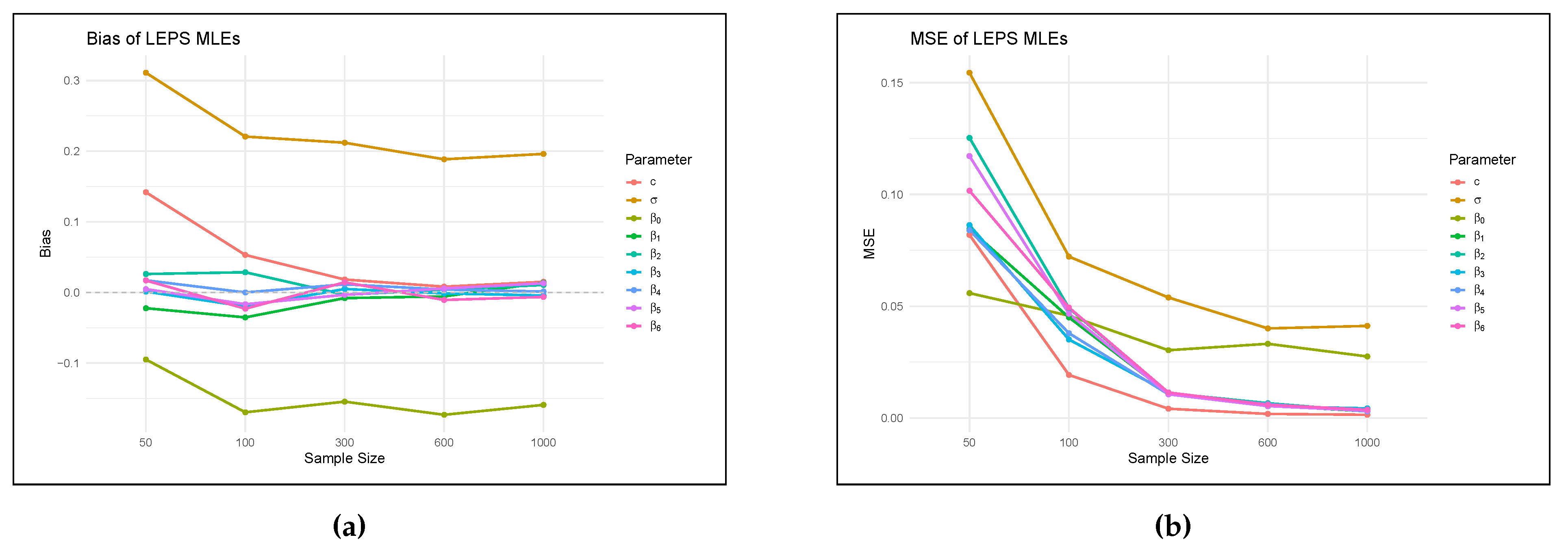
From Table 4, the simulation results for the MLEs of the LEPS regression model, with true parameters set as , , , , , , , , and , demonstrate distinct behaviors across varying sample sizes. For parameter c, its bias exhibits some fluctuation and does not consistently diminish towards zero, suggesting that larger sample sizes might be necessary for its full asymptotic properties to manifest, despite its MSE reducing significantly with increased sample size. By contrast, while the MSE for parameter consistently decreases, a persistent positive bias indicates the presence of a finite-sample bias even as precision improves. The intercept consistently shows a negative bias; although its MSE decreases, the magnitude of this bias does not decrease monotonically, possibly reflecting complex finite-sample dynamics. In contrast, the coefficients for the covariates ( to ) exhibit strong convergence of their mean estimates to the true values. Crucially, both the magnitude of their bias and their Mean Squared Error (MSE) consistently decrease with larger sample sizes, thereby affirming the expected asymptotic properties of MLEs for these parameters and confirming enhanced accuracy and precision. Overall, the findings align with the desirable asymptotic properties of MLEs for most parameters, indicating improved accuracy and precision as sample size increases. The very low incidence of simulation failures further attests to the excellent computational stability of the MLE procedure, an observation visually supported by Figure 7.
Figure (Figure 6) presents the simulation results for the MLEs of the LEPS regression model, illustrating the bias and Mean Squared Error (MSE) of the parameter estimates across varying sample sizes. Panel (a) displays the bias of the LEPS MLEs. It is evident that as the sample size increases from 50 to 1000, the bias for most parameters, including and the regression coefficients through , generally converges towards zero. This diminishing bias with increasing sample size suggests that the MLEs are asymptotically unbiased, a desirable property for these estimators. However, parameter c shows a more fluctuating bias that remains somewhat distant from zero, indicating that larger sample sizes than those explored might be required for its bias to fully dissipate, or that it exhibits a higher finite-sample bias. Panel (b) illustrates the MSE of the LEPS MLEs. Consistent with theoretical expectations for well-behaved estimators, the MSE for all parameters systematically decreases as the sample size increases. This trend confirms the asymptotic efficiency of the MLEs, indicating that the precision of the parameter estimates improves with larger datasets. The rate of decrease is notably steep for smaller sample sizes (e.g., from 50 to 300), after which the decline becomes more gradual, suggesting that while improvements in precision continue, the marginal gains diminish beyond a certain sample size within the simulated range. The overall pattern across both plots supports the statistical consistency of the LEPS MLEs, as both bias and variance (implicitly captured by MSE) generally decrease with increasing sample size.
7. Applications
In this section, we demonstrate the utility of the proposed LEPS regression model in explaining the impact of clinical factors on the lifetimes of COVID-19 patients. We also show its effectiveness in fitting traditional datasets, specifically times between failures for repairable items and the death rate of HIV/AIDS patients in Germany.
7.1. Fitting LEPS Regression Model to Lifetime of COVID-19 Patients
The dataset comprises the lifetime (in days) of 322 individuals diagnosed with COVID-19 through RT-PCR screening in Campinas, Brazil. These data were previously studied by [35]. A notable characteristic of this sample, is that approximately of the individuals have censored observations. This implies that for these participants, the event of death due to COVID-19 was not observed within the study’s follow-up period. For censored cases, we know only that their survival time extends beyond the recorded observation duration, meaning they were alive at the last point of contact or at the study’s conclusion. The variable `ind` serves as a unique, non-informative identifier for each participant in the dataset. Its role is solely for record management and to differentiate individual entries, carrying no inherent statistical value or order. Based on Equation (13), the variable ’censor’ is which is the crucial censoring indicator. It is a binary variable that takes a value of 0 if the observation for individual i is censored, indicating that the individual was alive at the end of the follow-up period or was lost to follow-up, without experiencing the event. Conversely, takes a value of 1 if the observed lifetime event, specifically death due to COVID-19, occurred for individual i. Age is representing the age of individual i, measured in full years. Age is a continuous covariate widely recognized as a significant demographic factor influencing the severity and outcomes of COVID-19 infection. The variable ’heart’ is . This binary variable would indicate the presence or absence of heart disease (e.g., cardiovascular disease, ischemic heart disease, heart failure) for individual i. A value of 1 would denote the presence of such a condition, and 0 its absence. Cardiac comorbidities are well-established risk factors for severe COVID-19. The variable ’asthma’ is , a binary variable which captures the presence or absence of asthma for individual i. A value of 1 would indicate a diagnosis of asthma, and 0 its absence. Respiratory conditions, including asthma, are frequently investigated as potential modifiers of COVID-19 severity. The variable ’diab’ is , a binary variable indicating the presence or absence of diabetes mellitus for individual i. A value of 1 signifies that the individual has a diagnosis of diabetes mellitus (or that this condition was reported), while 0 indicates the absence of diabetes or that this information was not available or not applicable. Diabetes is a common comorbidity consistently linked with increased risk of severe COVID-19 and adverse outcomes. The variable ’neuro’ , a binary variable which denote the presence or absence of a neurological condition for individual i. A value of 1 would signify the existence of such a condition, and 0 its absence. Neurological involvement and pre-existing neurological disorders have been identified in relation to COVID-19 outcomes. The variable ’obesity’ , a binary variable which indicates whether individual i is classified as obese. A value of 1 would signify obesity, and 0 its absence. Obesity is widely recognized as a significant risk factor for severe COVID-19 and increased mortality.
Figure (Figure 7a) represents the normal probability graph that shows that the lifetimes of the COVID-19 patients follow the normal distribution. Figure (Figure 7b) is the quantile residual plot against their index (the order of observations) in the dataset. From the plot, there are potential outliers as points lie below and above the lower and upper implicit boundaries (-3,3). Figure (Figure 7c) is the histogram of the age of the patients. It is evident from the histogram that the data is right-skewed.
For the fitting of the LEPS regression model to the lifetimes (in days) of COVID-19 patients, several established parametric regression models were selected for comparative analysis. These include the log-exponentiated power Chris-Jerry (LEPCJ) by [36], log-exponentiated power Akash (LEPA) by [37], log-power Prakaamy (LPP), log-exponentiated power Lindley (LEPL), log-power Rama (LPR), log-power Lomax (LPLo), log-power Zeghdoudi (LPZ), log-power Suja (LPSU), log-exponentiated power Ishita (LEPI), log-power Ishita (LPI), and the log-exponentiated Weibull (LEW) model.
Table (Table 5) shows comparisons of the model selection metrics of various distributions to the COVID-19 data. LEPS achieves the lowest Akaike Information Criterion (AIC = 426.4954), Consistent AIC (CAIC = 427.3471), and Hannan-Quinn Information Criterion (HQIC = 440.0577), and thus ranks first by consequence. LEPI and LEW models follow with slightly higher values in these metrics. In contrast, models such as LPP and LEPR have very much larger information criteria values, which refer to poorer fit. Bayesian Information Criterion (BIC) ranks LPZ last among all the best-fitting models, even though its AIC and CAIC values are higher than those of LEPS. Overall, the results reveal that the LEPS distribution presents the most consistent and best-fitting model for the data among the competitors under consideration.
For each distributional model in Table (Table 6), the regression model is
The statistically significant predictors (meaning ) within models tend to consist of age, heart disease, and neurological condition, and sometimes diabetic condition, which are constant negative or positive effects depending on the model. The signs of coefficients define the effect direction: age (usually negative and significant), heart disease (negative and significant), neurological condition (negative and significant in most models), Others (asthma, diabetic condition and obesity) vary less in significance. Parameter c distinguishes between models and is linked with the shape or flexibility of fit of the distribution, and is representative of scale with varying precision.
For the LEPS model, the regression model for the lifetimes (in days) of COVID-19 patients () is given by:
Standard errors are given in parentheses, and p-values are shown in brackets below:
The scale and shape parameters of the LEPS distribution are These are specific to the LEPS distribution; where
- (i)
- Intercept (): Estimated lifetime for the baseline patient with all predictors at zero (i.e. youngest age, no heart disease, no asthma, no diabetes, no neurological condition, no obesity) is about 4 years and 6 months.
- (ii)
- Age (): For every additional year of age, the lifetime is expected to decrease by roughly 0.018 years, holding all else equal. This suggests a negative correlation between survival time and age.
- (iii)
- Heart disease (): Patients with heart disease suffers a lifetime reduction by about 0.31 years.
- (iv)
- Asthma (): Asthma appears to be positively correlated with lifetime, increasing it by about 0.088 years but it is not significant statistically since (p-value ).
- (v)
- Diabetes (): lifetime for diabetic patients is significantly low at about 0.54 years, suggesting diabetes seriously reduces the life expectancy of a COVID-19 patient.
- (vi)
- Neurological condition (): Neurological conditions also decrease lifetime by about 0.44 years.
- (vii)
- Obesity (): Obesity has a very weak negative effect on lifetime, but the effect is small and not statistically significant.
This model quantifies to what degree clinical parameters influence COVID-19 patients’ lifetimes through differences in survivals, which identifies high-risk groups. Across all the models considered, a consistent pattern emerges regarding the significance of covariates. Specifically, the parameters , , and were found to be statistically significant in every model. These parameters correspond to age, heart disease, and neurological condition, respectively, suggesting their strong association with the response variable under study. For models such as LEPS, LEPCJ, LEPA, LEPL, LEPR, LPL, LEPI, and LEW, the parameters c, , , , , and were consistently not significant. This implies that these covariates do not have a meaningful contribution to the outcome in these models. In contrast, for the LPP, LPZ, LEPSU, and LPI models, the parameter c is not applicable, yet the insignificance of , , , , and remains consistent. It is noteworthy that despite the structural differences in the models (such as the presence or absence of parameter c), the core set of significant parameters (, , and ) remains unchanged. This reinforces the robustness of their influence and suggests that interventions or predictions based on these variables are likely to be reliable across various modeling frameworks. The repeated insignificance of parameters like , , , and across models indicates that these variables may be redundant or have weak explanatory power in the context of this analysis. It may be beneficial in future studies to consider removing or replacing these covariates to streamline model complexity without sacrificing predictive accuracy.
The 95% confidence intervals for the parameters are computed with the following formula, For instance, in the LEPS model, the coefficient for age () had a , indicating a statistically significant and negative association with lifetime. Confidence intervals for other parameters provide similar insights and can be found in Tables (Table 7) and (Table 8). Above all, this consistency in parameter significance across different link functions and error structures provides strong evidence for the reliability of key predictors and offers direction for model refinement. Confidence intervals were computed for each parameter estimate to assess the precision of the estimates.
7.2. Fitting EPS to Reliability Data
The first data set represent the times between failures for repairable items initially studied by [38] and reported in Table (Table 9). The second data set is Death rate due to HIV/AIDS in Germany from year 2000 to 2020 reported in https://platform.who.int/mortality/themes/theme-details/topics/indicator-groups/indicator-group-details/MDB/hiv-aids and presented in Table (Table 10). In Table (Table 11), we present a summary of basic statistics to gain insight from the two data sets. From Table (Table 11), the repairs times dataset is smaller on its mean (0.0154) and median (0.0124), and has a steep right skew (skewness = 1.2955) that indicates a longer right tail. It is also smaller with an IQR of 0.0123 and a range of 0.0462. Two outliers indicate extreme values. A high kurtosis of 4.3192 indicates a more pointed distribution with heavier tails. In contrast, the HIV/AIDS mortality rate data set has a mean of 0.5203, median of 0.5395, and is very slightly left-skewed with skewness -0.3335, showing slight asymmetry toward smaller values. The inter-quartile range (IQR) is 0.1590, with a total range of 0.3786, and a standard deviation of 0.1090, showing moderate variability. Its kurtosis of 2.1101 shows a very slightly flatter distribution than normal.
The proposed EPS distribution is compared with new generalized logistic-x transformed exponential (NGLXTE) distribution introduced by [39], Logistic-Weibull distribution by [40], power Zeghdoudi distribution by [41], power Ishita distribution by [42], power Prakaamy distribution by [43], power Rama distribution by [44] and Power Lomax distribution introduced by [45]. The model selection criteria are the Akaike information criterion (AIC), consistent Akaike information criterion (CAIC), Bayesian information criterion (BIC) and Hannan-Quinn information criterion (HQIC) which are computed using;
where is the log-likelihood function in Equation (), k is the number if parameters, n represents the sample size and is the vector of parameters; for the EPS model, For goodness of fit test, let an be an ordered random sample from the EPS , where c, and are unknown; the Cramér-von Mises , Anderson-Darling and Kolmogorov-Smirnov statistics are computed using the following;

Table 12.
Model Assessment and Goodness of Fit Criteria for the Data sets
| Data | Distribution | LL | AIC | CAIC | BIC | HQIC | P-value | |||
|---|---|---|---|---|---|---|---|---|---|---|
| Data-I | EPS | 98.54 | -191.0839 | -190.1608 | -186.8803 | -189.7391 | 0.0178 | 0.1346 | 0.0660 | 0.9995 |
| NGLXTE | 96.82 | -189.6349 | -189.1904 | -186.8325 | -188.7383 | 0.0712 | 0.5074 | 0.1219 | 0.7643 | |
| Logistic-Weibull | 97.74 | -189.4824 | -188.5593 | -185.2788 | -188.1376 | 0.0303 | 0.1958 | 0.0738 | 0.9968 | |
| Power Zeghdoudi | 231.89 | -459.7825 | -459.3380 | -456.9801 | -458.8860 | 0.0189 | 0.1435 | 0.0661 | 0.9994 | |
| Power Ishita | 98.24 | -192.4895 | -192.0450 | -189.6871 | -191.5929 | 0.0280 | 0.2115 | 0.0749 | 0.9960 | |
| Power Prakaamy | 98.24 | -192.4895 | -192.045 | -189.6871 | -191.5929 | 0.0280 | 0.2115 | 0.0749 | 0.9960 | |
| Power Rama | -196.4895 | -192.4895 | -192.045 | -189.6871 | -191.5929 | 0.0220 | 0.2116 | 0.0748 | 0.9960 | |
| Power Lomax | 98.46 | -190.9299 | -190.0068 | -186.7263 | -189.5851 | - | - | 367.17 | ||
| Data-II | EPS | 17.95 | -29.8916 | -28.4798 | -26.7580 | -29.2115 | 0.0225 | 0.1958 | 0.0868 | 0.9932 |
| NGLXTE | 17.84 | -31.6816 | -31.0149 | -29.5925 | -31.2282 | 0.0275 | 0.2202 | 0.0945 | 0.9827 | |
| Logistic-Weibull | 15.77 | -25.5328 | -24.1211 | -22.3993 | -24.8528 | 0.0923 | 0.6032 | 0.1170 | 0.9044 | |
| Power Zeghdoudi | 31.70 | -59.4087 | -58.7420 | -57.3196 | -58.9553 | 0.0466 | 0.3275 | 0.1054 | 0.9546 | |
| Power Ishita | 17.79 | -31.5737 | -30.9070 | -29.4846 | -31.1203 | 0.0326 | 0.2473 | 0.0999 | 0.9710 | |
| Power Prakaamy | 17.79 | -31.5738 | -30.9072 | -29.4848 | -31.1205 | 0.0326 | 0.2473 | 0.0999 | 0.9710 | |
| Power Rama | -35.57 | -31.5714 | -30.9047 | -29.4823 | -31.1180 | 0.0326 | 0.2474 | 0.1000 | 0.9707 | |
| Power Lomax | 17.78 | -29.5634 | -28.1516 | -26.4298 | -28.8833 | 0.0756 | 0.5523 | 0.9074 | 2.2 |
Model fit was checked using the log-likelihood (LL), Akaike Information Criterion (AIC), Bayesian Information Criterion (BIC), Corrected AIC (CAIC), and Hannan-Quinn Information Criterion (HQIC). Models with higher log-likelihood and lower information criteria are considered better for parameter estimation. In Data I, Power Zeghdoudi distribution possessed the highest log-likelihood (LL = 231.89) and lowest AIC, BIC, CAIC, and HQIC, thereby indicating the best parameter estimation fit. However, the log-likelihood value is significantly higher than the rest, and the disparity may reflect an inconsistency in scaling or computation error that needs to be verified. Omitting Power Zeghdoudi, the Power Ishita and Power Prakaamy distributions were found to perform competitively with similar low information criteria. The EPS and Logistic-Weibull models also showed good performance with good values of log-likelihood and acceptable values of information criteria. The Power Lomax model was far worse based on very poor goodness-of-fit statistics and low log-likelihood. In Data II, the Power Zeghdoudi model again produced the best estimation performance, with maximum LL (31.70) and minimum information criteria. The next best were NGLXTE, Power Ishita, and Power Prakaamy, all of whom had closely competing values. The EPS and Logistic-Weibull models ranked slightly below in parameter estimation accuracy. Goodness-of-fit was assessed according to the Cramér–von Mises (W), Anderson–Darling (A), and Kolmogorov–Smirnov (KS) statistics and their corresponding p-values. Small W, A, KS statistics and large p-values for models indicate closer fit to empirical data. For Data I, all of EPS, Power Zeghdoudi, Power Ishita, Power Prakaamy, and Logistic-Weibull distributions provided excellent fit with very small KS values (0.066 to 0.075) and very large p-values (larger than 0.996). Among them, the EPS model provided the largest p-value of 0.9995, indicating the best fit to empirical distribution. On the contrary, the Power Lomax distribution provided very poor fit with very large KS statistics and a p-value near zero. Even in Data II, the same performance pattern was observed. The distributions of EPS, Power Zeghdoudi, Power Ishita, Power Prakaamy, and NGLXTE all had low KS values (0.0868 to 0.1000) and high p-values (0.9707 to 0.9932), which suggest very good reliability. The Power Lomax distribution again had very high KS statistics and essentially zero p-values, which suggest poor fit.
Table 13 presents the maximum likelihood estimates (MLEs) and standard errors of the parameters of various statistical distributions fitted to Data-I and Data-II. For the EPS distribution, the parameter estimates vary significantly across datasets, with , , and taking higher values and standard errors in Data-I, reflecting higher variability. The NGLXTE model yields more stable estimates with relatively smaller standard errors, particularly for Data-II, reflecting higher model accuracy. The Logistic-Weibull distribution contains large standard errors in both data, particularly in and , which could indicate issues with parameter identifiability or fit to the data. The Power Zeghdoudi, Power Ishita, Power Prakaamy, and Power Rama distributions yield stable estimates between Data-I and Data-II, particularly in and , with Data-II providing lower standard errors, indicating more precise inference. Lastly, the Power Lomax distribution displays extreme differences between datasets in parameter size and standard error, most notably in and , with Data-II estimates being considerably larger. Overall, the results indicate that parameter estimates and their errors vary quite noticeably between models and datasets, with certain distributions exhibiting more stability and precision for specific data.
In Figure (Figure 8), the data plot for Data-I overlays a violin plot with an embedded boxplot, and a histogram with a superimposed density curve. The histogram indicates right-skewness with dense low values and an elongated tail. The red density curve verifies the skewness and identifies the peak at a low value. The violin plot also visually supports the shape of the distribution. The box plot shows a small median and narrowed interquartile range (IQR), which is characteristic of right-skewness. For Data-II, the histogram shows right skewness, though perhaps less pronounced than for Data-I. The density curve supports this skewness. The violin and boxplot show slightly higher median and IQR than for Data-I. In Figure (Figure 9), plot for Data-I; Empirical CDF (red line) closely matches the EPS CDF fitted (black line / dots), indicating a good fit. The same assertion for Data-II on the basis of a similar trend as Data-I since empirical and EPS CDFs closely match. bThe empirical survival function (red line) closely matches the theoretical survival function of the EPS. The TTT plot of Data-I in Figure (Figure 10) is concave up, reflecting increasing hazard rate. Similar to Data-I, the TTT plot of Data-II reflects increasing hazard rate behavior. Data-I PP Plot’s red dots are close to the diagonal, which provides a good fit of the EPS distribution. For Data-II PP Plot, dots are also close to the diagonal and provide a strong fit for Data-II. In Figure (Figure 11), the quantiles of Data-I coincide closely with quantiles of the EPS distribution with slight discrepancies. Similarly, Data-II quantiles follow theoretical EPS quantiles closely, confirming a close fit. Both data sets are right-skewed and appear overall more concentrated towards small values for Data-I. Both exhibit increasing hazard rates as confirmed by TTT plots. The EPS distribution gives a good and consistent fit to both data sets with respect to: Empirical CDFs and survival functions, PP plots (probability correspondence), and QQ plots (quantile correspondence). Robustness of the overall fit with all the diagnostics provides the evidence of the appropriateness of the EPS distribution as the model for both the data sets.
8. Conclusion
The EPS distribution, proposed here, has strong modeling flexibility and empirical relevance for lifetime and reliability data. Through thorough structural analysis and simulation, the distribution has been proven to model a broad spectrum of density and hazard function shapes—varying from unimodal and skewed to bathtub and monotonic behaviors. Simulation results show that while the MLEs can become biased in small samples, especially for specific parameter settings, the estimators become more stable and accurate as the sample size increases. Application of the EPS model on two real data sets—repair time and HIV/AIDS mortality rates—documents its pragmatic solidness. In both cases, the EPS distribution shows an excellent fit, performing competitively or better than other proven distributions such as Power Ishita, Logistic-Weibull, and Power Zeghdoudi according to likelihood-based criteria and goodness-of-fit tests. Diagnostic plots (QQ, PP, CDF, and TTT plots) graphically authenticate the better or competitive fit of the model. Hence, the EPS distribution is a powerful member of the family of flexible life-time models, highly suitable in the broad range of applied contexts in survival analysis, reliability analysis, and public health research. Its extension to regression further broadens its suitability for covariate-dependent response modeling.
Author Contributions
For research articles with several authors, a short paragraph specifying their individual contributions must be provided. The following statements should be used “Conceptualization, X.X. and Y.Y.; methodology, X.X.; software, X.X.; validation, X.X., Y.Y. and Z.Z.; formal analysis, X.X.; investigation, X.X.; resources, X.X.; data curation, X.X.; writing—original draft preparation, X.X.; writing—review and editing, X.X.; visualization, X.X.; supervision, X.X.; project administration, X.X.; funding acquisition, Y.Y. All authors have read and agreed to the published version of the manuscript.”, please turn to the CRediT taxonomy for the term explanation. Authorship must be limited to those who have contributed substantially to the work reported.
Funding
This work was supported and funded by the Deanship of Scientific Research at Imam Mohammad Ibn Saud Islamic University (IMSIU) (grant number IMSIU-DDRSP2501).
Data Availability Statement
This study used publicly available data and codes which can be accessed from https://github.com/obulezi12345-svg/exponentiated-power-shanker-R-codes
Conflicts of Interest
The authors declare that there is no competing interest.
References
- Shanker, R. Shanker distribution and its applications. International journal of statistics and Applications 2015, 5, 338–348. [Google Scholar] [CrossRef]
- Lindley, D.V. Fiducial distributions and Bayes’ theorem. Journal of the Royal Statistical Society. Series B (Methodological), 1958; 102–107. [Google Scholar]
- Onyekwere, C.K.; Obulezi, O.J. Chris-Jerry distribution and its applications. Asian Journal of Probability and Statistics 2022, 20, 16–30. [Google Scholar] [CrossRef]
- Odom, C.; Ijomah, M. Odoma distribution and its application. Asian journal of probability and statistics 2019, 4, 1–11. [Google Scholar] [CrossRef]
- KK, S. Pranav distribution with properties and its applications. Biom Biostat Int J 2018, 7, 244–254. [Google Scholar]
- Shanker, R. Aradhana distribution and its applications. International Journal of Statistics and Applications 2016, 6, 23–34. [Google Scholar] [CrossRef]
- Ekemezie, D.F.N.; Obulezi, O.J. The Fav-Jerry Distribution: Another Member in the Lindley Class with Applications. Earthline Journal of Mathematical Sciences 2024, 14, 793–816. [Google Scholar] [CrossRef]
- Ghitany, M.E.; Al-Mutairi, D.K.; Balakrishnan, N.; Al-Enezi, L.J. Power Lindley distribution and associated inference. Computational Statistics & Data Analysis 2013, 64, 20–33. [Google Scholar] [CrossRef]
- Shanker, R.; Shukla, K.K. Power Shanker distribution and its application. Türkiye Klinikleri Biyoistatistik 2017, 9, 175–187. [Google Scholar] [CrossRef]
- Embrechts, P.; Klüppelberg, C.; Mikosch, T. Modelling Extremal Events: for Insurance and Finance; Springer, 1997.
- Kotz, S.; Nadarajah, S. Extreme Value Distributions: Theory and Applications; Imperial College Press, 2000.
- Azzalini, A. A class of distributions which includes the normal ones. Scandinavian Journal of Statistics 1985, 12, 171–178. [Google Scholar]
- Aryal, G.R.; Nadarajah, S. Skew t-distribution and its applications. Statistics 2005, 39, 55–76. [Google Scholar]
- McLachlan, G.J.; Peel, D. Finite Mixture Models; Wiley-Interscience, 2000.
- Rasmussen, C.E. The infinite Gaussian mixture model. PhD thesis, University of Cambridge, 1999.
- Lambert, D. Zero-inflated Poisson regression, with an application to defects in manufacturing. Technometrics 1992, 34, 1–14. [Google Scholar] [CrossRef]
- Ridout, M.S.; Demetrio, C.G.; Hinde, J. Count data models with heterogeneity: An application to claim frequency data. Biometrical Journal 2001, 43, 441–452. [Google Scholar]
- Jones, M.C. Kumaraswamy distribution: properties and applications. International Journal of Statistical Modeling 2009, 8, 281–298. [Google Scholar]
- Cordeiro, G.M.; de Castro, M.H. The beta generalized Kumaraswamy distribution. Journal of Statistical Computation and Simulation 2011, 81, 891–907. [Google Scholar]
- Mudholkar, G.S.; Srivastava, D.K.; Freimer, M. The exponentiated Weibull family: A reanalysis of the bus-motor-failure data. Technometrics 1996, 38, 253–256. [Google Scholar] [CrossRef]
- Aarset, M.V. How to identify a bathtub hazard rate. IEEE Transactions on Reliability 1987, 36, 106–108. [Google Scholar] [CrossRef]
- Box, G.E.P.; Jenkins, G.M. Time Series Analysis: Forecasting and Control; Holden-Day, 1976.
- Joe, H. Multivariate Models and Dependence Concepts; Chapman and Hall/CRC, 1997.
- Klein, J.P.; Moeschberger, M.L. Survival Analysis: Techniques for Censored and Truncated Data; Springer, 2003.
- Tobin, J. Estimation of relationships for limited dependent variables. Econometrica 1958, 26, 24–36. [Google Scholar] [CrossRef]
- Gelman, A.; Carlin, J.B.; Stern, H.S.; Dunson, D.B.; Vehtari, A.; Rubin, D.B. Bayesian Data Analysis, 3rd ed.; Chapman and Hall/CRC, 2013.
- McCulloch, C.E.; Searle, S.R.; Neuhaus, J.M. Generalized, Linear, and Mixed Models; Wiley, 2001.
- Zhou, F.; Yu, T.; Du, R.; Fan, G.; Liu, Y.; Liu, Z.; Xiang, J.; Wang, Y.; Song, B.; Gu, X.; et al. Clinical course and risk factors for mortality of adult inpatients with COVID-19 in Wuhan, China: a retrospective cohort study. The Lancet 2020, 395, 1054–1062. [Google Scholar] [CrossRef]
- Guan, W.j.; Liang, W.h.; Zhao, Y.; Liang, H.r.; Chen, Z.s.; Li, Y.m.; Liu, X.q.; Chen, R.c.; Tang, C.l.; Wang, T.; et al. Comorbidity and its impact on 1590 patients with COVID-19 in China: a nationwide analysis. European Respiratory Journal 2020, 55. [Google Scholar] [CrossRef]
- Chen, T.; Wu, D.; Chen, H.; Yan, W.; Yang, D.; Chen, G.; Ma, K.; Xu, D.; Yu, H.; Wang, H.; et al. Clinical characteristics of 113 deceased patients with coronavirus disease 2019: retrospective study. BMJ 2020, 368. [Google Scholar] [CrossRef]
- Huang, C.; Wang, Y.; Li, X.; Ren, L.; Zhao, J.; Hu, Y.; Zhang, L.; Fan, G.; Xu, J.; Gu, X.; et al. Clinical features of patients infected with 2019 novel coronavirus in Wuhan, China. The Lancet 2020, 395, 497–506. [Google Scholar] [CrossRef] [PubMed]
- Sardu, C.; D’Onofrio, N.; Biondi-Zoccai, G.; Ferraraccio, F.; Rizzo, M.R.; Barbieri, M.; Ruggiero, R.; Marfella, R.; Paolisso, G. Outcome of patients with diabetes mellitus affected by COVID-19: experience from an Italian hospital. Diabetes research and clinical practice 2020, 162, 108137. [Google Scholar]
- Durrans, S.R. Distributions of fractional order statistics in hydrology. Water Resources Research 1992, 28, 1649–1655. [Google Scholar] [CrossRef]
- Lehmann, E.L. The power of rank tests; Springer, 2012.
- Ferreira, A.A.; Cordeiro, G.M. The exponentiated power Ishita distribution: Properties, simulations, regression, and applications. Chilean Journal of Statistics (ChJS) 2023, 14. [Google Scholar] [CrossRef]
- Obulezi, O.J.; Ujunwa, O.E.; Anabike, I.C.; Igbokwe, C.P. The exponentiated power Chris-Jerry distribution: properties, regression, simulation and applications to infant mortality rate and lifetime of COVID-19 patients. TWIST 2023, 18, 328–337. [Google Scholar]
- Nwankwo, M.P.; Nwankwo, B.C.; Obulezi, O.J. The Exponentiated Power Akash Distribution: Properties, Regression, and Applications to Infant Mortality Rate and COVID-19 Patients’ Life Cycle. Annals of Biostatistics and Biometric Applications 2023, 5, 1–12. [Google Scholar]
- Murthy, D.P.; Xie, M.; Jiang, R. Weibull models; John Wiley & Sons, 2004.
- Obulezi, O.J.; Obiora-Ilouno, H.O.; Osuji, G.A.; Kayid, M.; Balogun, O.S. A new family of generalized distributions based on logistic-x transformation: sub-model, properties and useful applications. Research in Statistics 2025, 3, 2477232. [Google Scholar] [CrossRef]
- Chaudhary, A.K.; Kumar, V. The Logistic-Weibull distribution with Properties and Applications. IOSR Journal of Mathematics 2021, 17, 32–41. [Google Scholar]
- Messaadia, H.; Zeghdoudi, H. Zeghdoudi distribution and its applications. International Journal of Computing Science and Mathematics 2018, 9, 58–65. [Google Scholar] [CrossRef]
- Shukla, K.K.; Shanker, R. Power Ishita distribution and its application to model lifetime data. Statistics in Transition new series 2018, 19. [Google Scholar] [CrossRef]
- Shukla, K.K.; Shanker, R. Power Prakaamy distribution and its applications. International Journal of Computational and Theoretical Statistics 2020, 7. [Google Scholar]
- Abebe, B.; Tesfay, M.; Eyob, T.; Shanker, R. A two-parameter power Rama distribution with properties and applications. Biometrics and Biostatistics International Journal 2019, 8, 6–11. [Google Scholar]
- Rady, E.H.A.; Hassanein, W.; Elhaddad, T. The power Lomax distribution with an application to bladder cancer data. SpringerPlus 2016, 5, 1–22. [Google Scholar] [CrossRef]
Figure 1.
The PDF of EPS
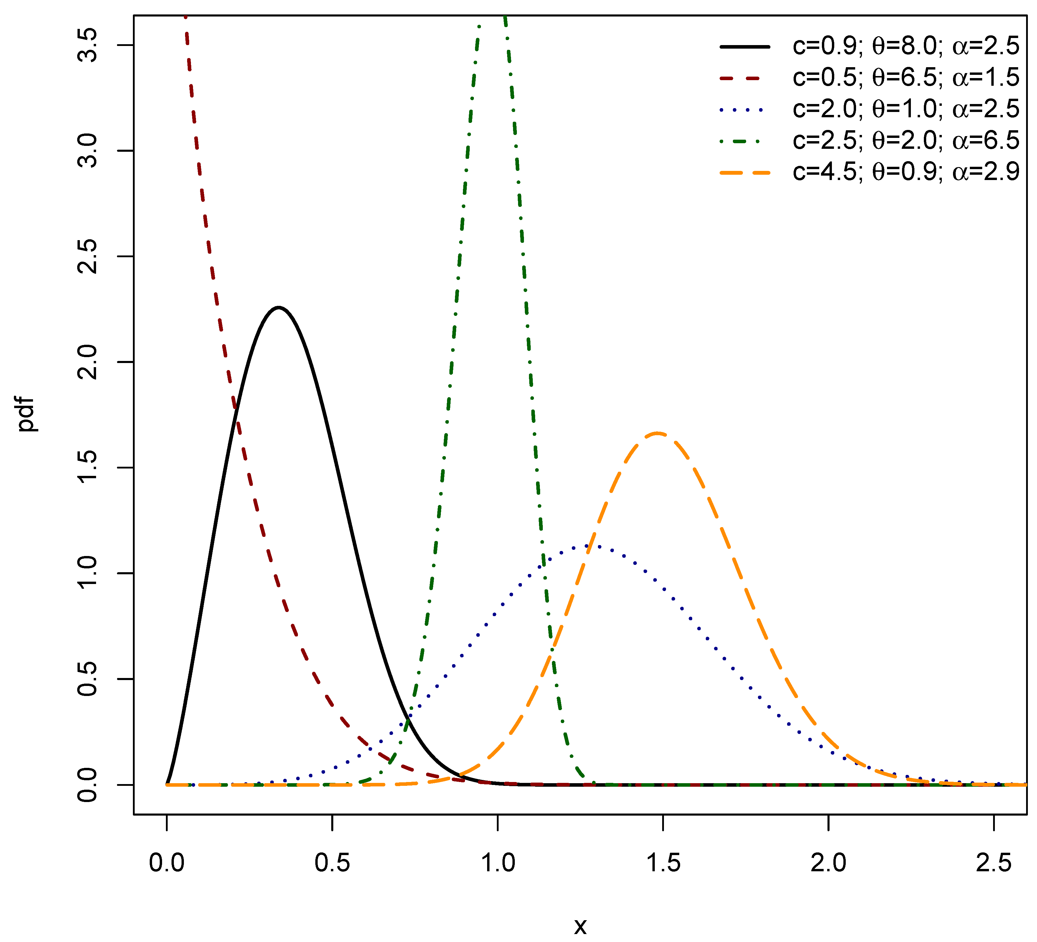
Figure 2.
The PDF of EPS
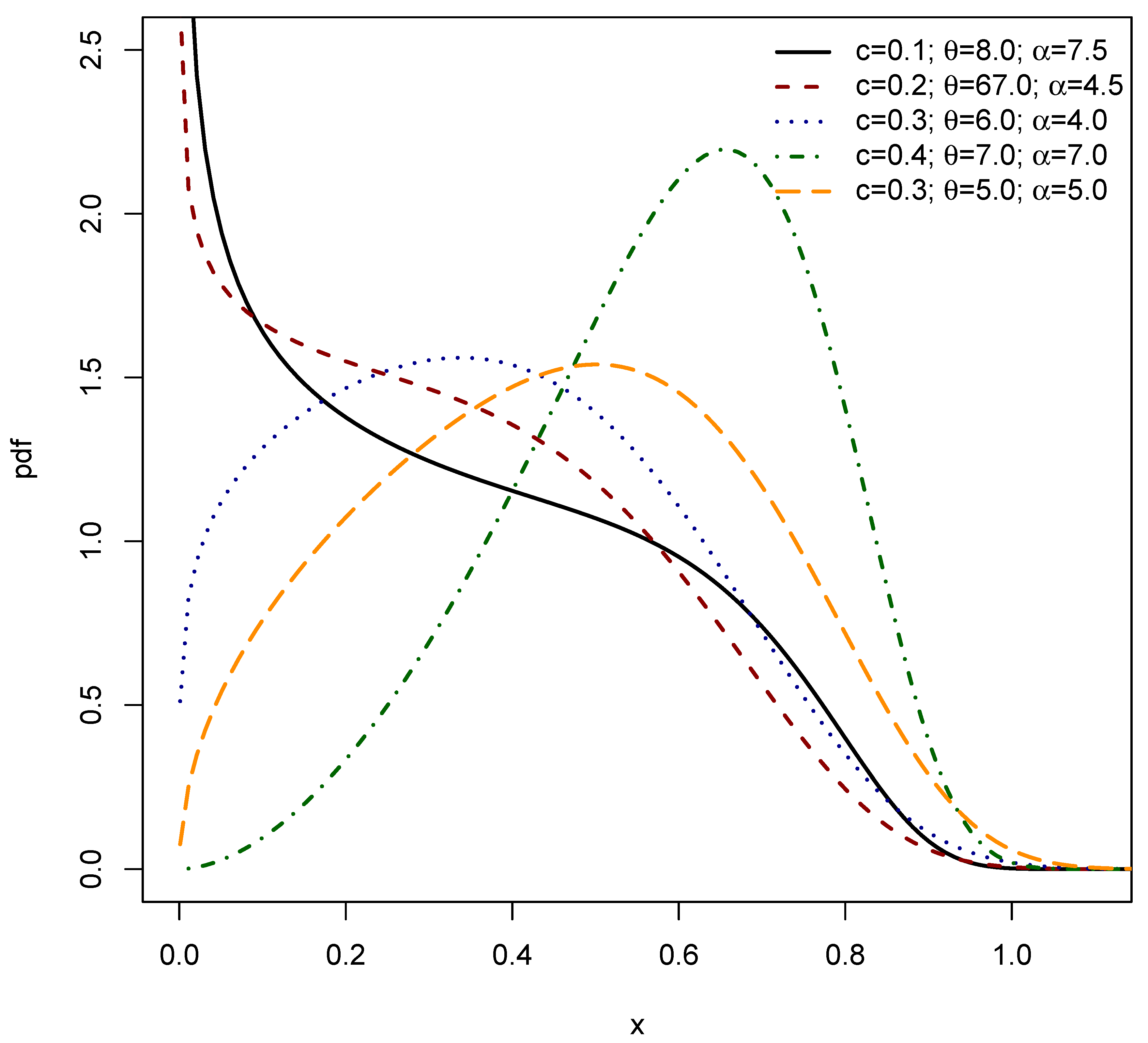
Figure 3.
The HRF of EPS
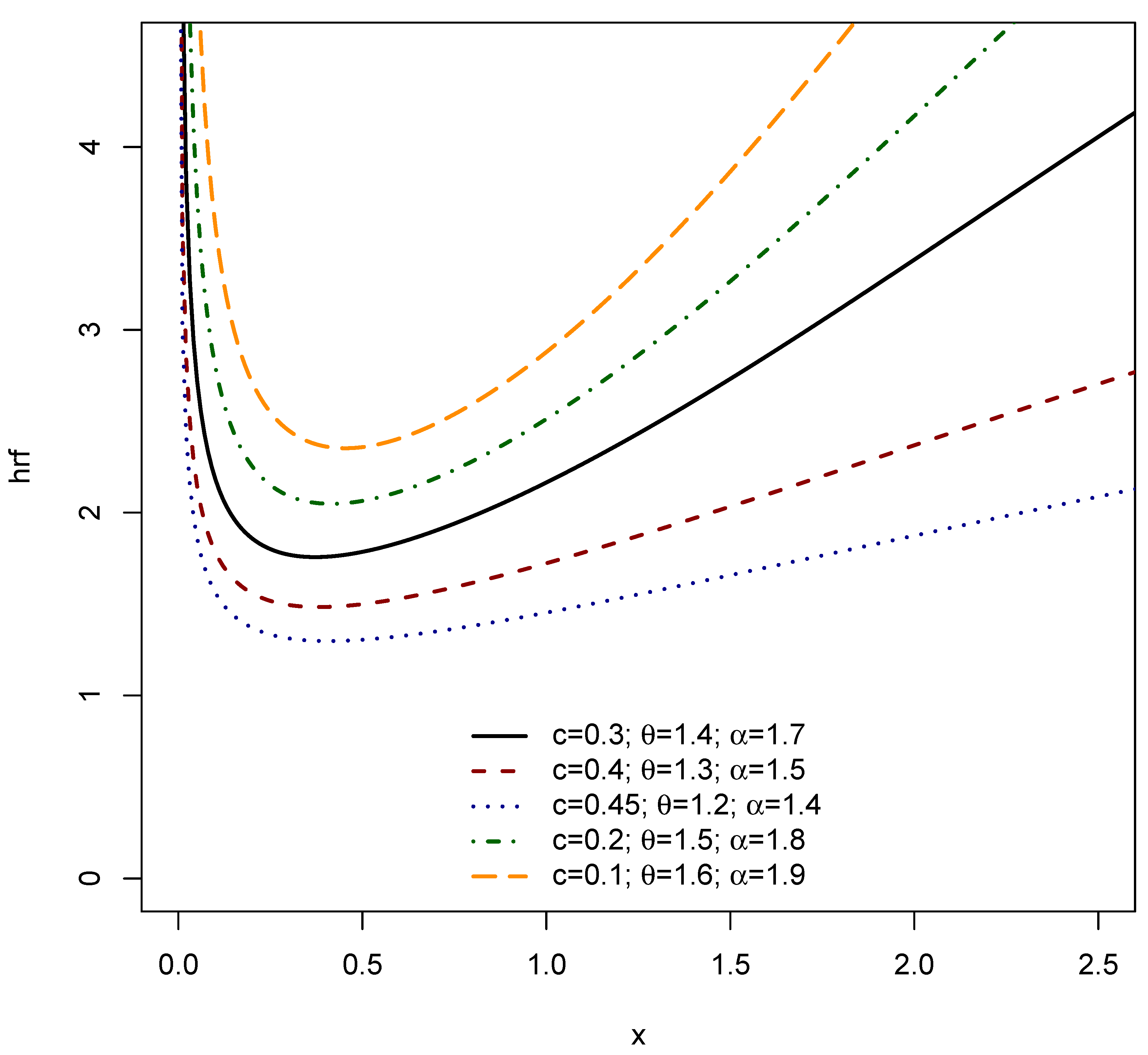
Figure 4.
The HRF of EPS
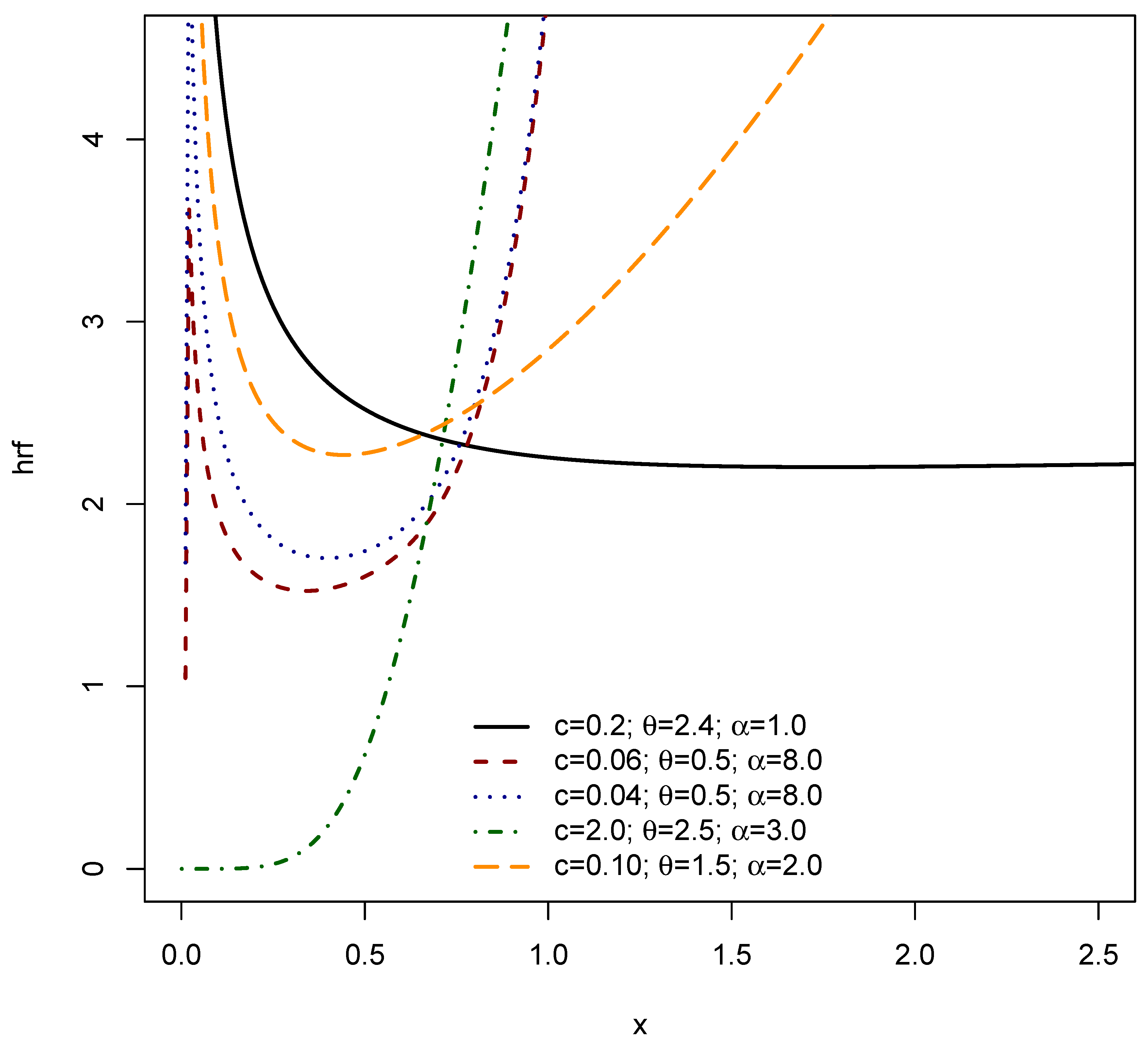
Figure 5.
Mean, Variance, Skewness, and Kurtosis
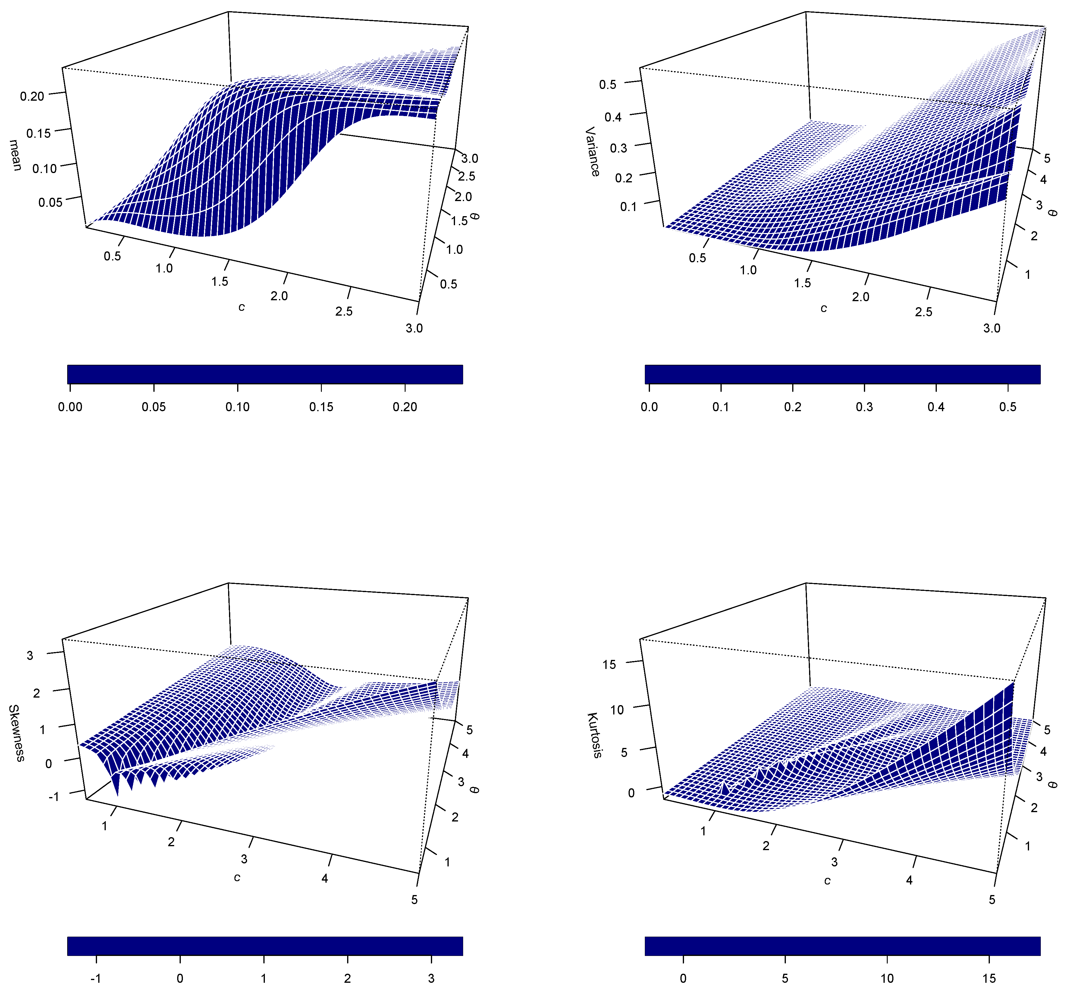
Figure 7.
(a) Normal probability plot (b) Index plot (c) Histogram for age
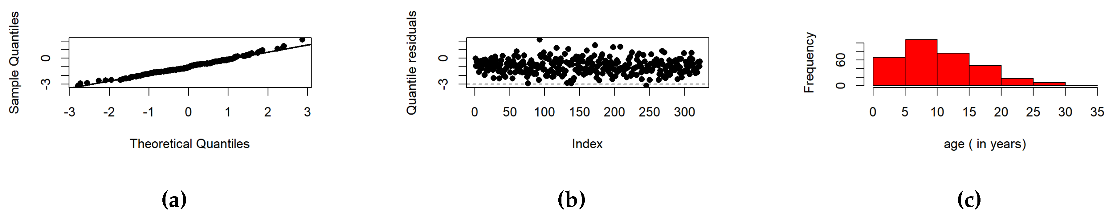
Figure 8.
Boxplots superimposed on Violin and Density plots superimposed on Histogram
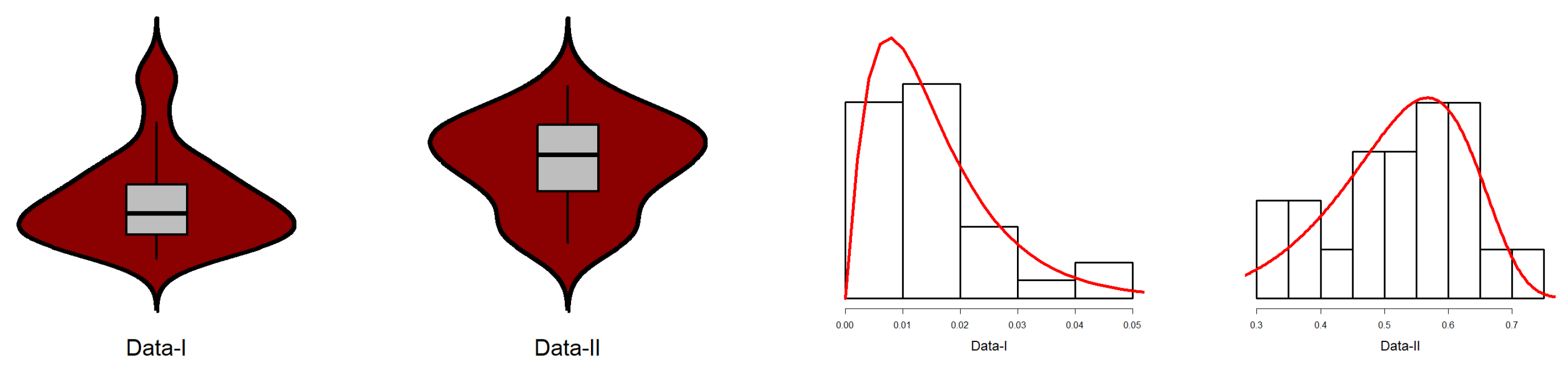
Figure 9.
Empirical CDF with superimposed EPS CDF, Empirical S(x) with superimposed EPS Survival Function
Figure 9.
Empirical CDF with superimposed EPS CDF, Empirical S(x) with superimposed EPS Survival Function
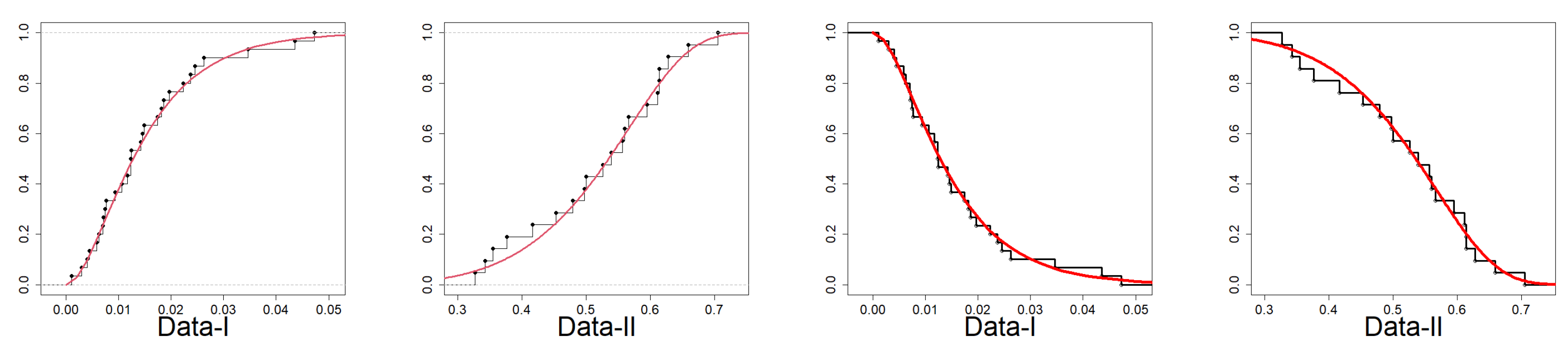
Figure 10.
TTT and PP Plots
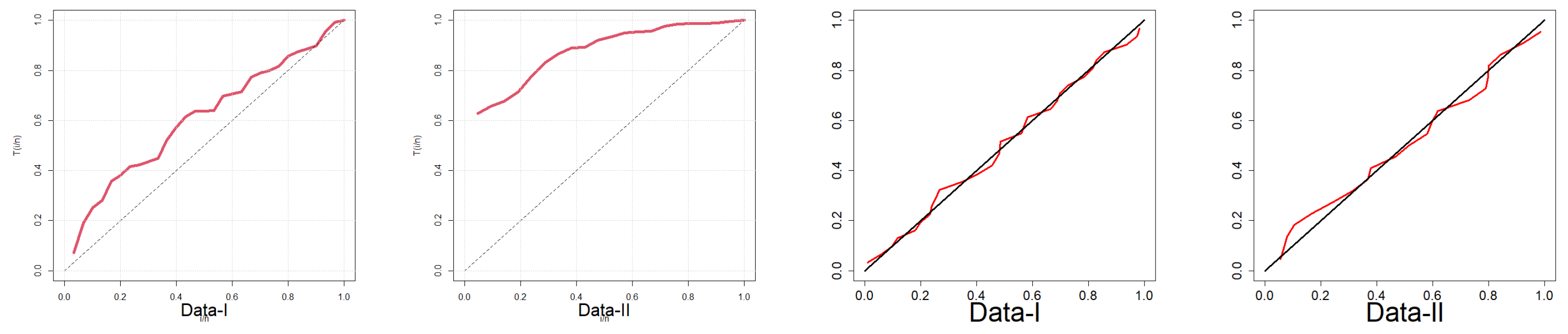
Figure 11.
QQ plots
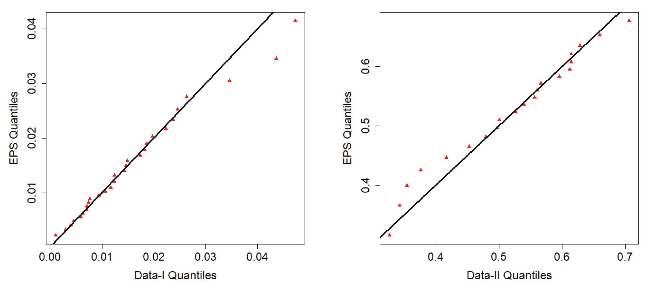
Table 1.
Emerging Data Behaviors, Standard Limitations, and Advanced Models
| Behavior | Examples | Standard Limitation | Advanced Models | References |
|---|---|---|---|---|
| Heavy Tails | Financial returns, insurance claims | Normal, exponential decay too quickly | Pareto, t-distribution, Generalized Pareto Distribution (GPD), Log-Cauchy, Stable distributions | [10,11] |
| Skewness | Income, survival times | Normal/logistic are symmetric | Skew-normal, Skew-t, Exponentiated, Transmuted models | [12,13] |
| Multimodality | Gene expression, survey responses | Standard distributions are unimodal | Mixture models, Dirichlet processes, Kernel Density Estimation (KDE) | [14,15] |
| Zero-inflation | Doctor visits, insurance claims | Poisson underestimates zeros | Zero-inflated Poisson, Zero-inflated Negative Binomial | [16,17] |
| Complex bounded shapes | Proportions, rates (0 to 1) | Beta/uniform lack shape flexibility | Kumaraswamy, Beta-Kumaraswamy, Generalized Beta (GB) family | [18,19] |
| Non-monotonic hazard | Reliability/survival data | Weibull assumes monotonic hazard | Exponentiated Weibull, Bathtub models | [20,21] |
| Dependence (Temporal/Spatial) | Sensor data, climate, markets | Assumes independence | ARIMA, GARCH, Spatial Autoregressive (SAR) models, Copulas | [22,23] |
| Censoring or Truncation | Survival, income data | Assumes complete data | Tobit models, Kaplan-Meier estimator, Cox proportional hazards model | [24,25] |
| Nonlinear/Mixed structures | Random or hierarchical effects | Cannot capture heterogeneity | Generalized Linear Mixed Models (GLMMs), Bayesian Hierarchical Models | [26,27] |
Table 2.
Simulation Result I for the EPS Model
| True Population Parameter | n | AE | Bias | MSE | Failure | |
|---|---|---|---|---|---|---|
|
and |
50 | c | 4.01214 | 2.76214 | 1805.52 | 2 |
| 3.21083 | 0.21083 | 1.07584 | ||||
| 2.70836 | 0.45836 | 3.05114 | ||||
| 100 | c | 1.48190 | 0.23193 | 0.94771 | 0 | |
| 3.07120 | 0.07120 | 0.28288 | ||||
| 2.40114 | 0.15114 | 0.58128 | ||||
| 300 | c | 1.29588 | 0.04588 | 0.14002 | 0 | |
| 3.02794 | 0.02794 | 0.07585 | ||||
| 2.30830 | 0.05830 | 0.13499 | ||||
| 600 | c | 1.27276 | 0.02276 | 0.05977 | 0 | |
| 3.01246 | 0.01246 | 0.03454 | ||||
| 2.27485 | 0.02485 | 0.05943 | ||||
|
and |
50 | c | 2.39687 | 1.19687 | 102.66400 | 0 |
| 2.64503 | 0.14503 | 0.74596 | ||||
| 2.06780 | 0.31780 | 1.37844 | ||||
| 100 | c | 1.53352 | 0.33352 | 20.05157 | 0 | |
| 2.55056 | 0.05056 | 0.29395 | ||||
| 1.89479 | 0.14479 | 0.41803 | ||||
| 300 | c | 1.25556 | 0.05556 | 0.13416 | 0 | |
| 2.51623 | 0.01623 | 0.07365 | ||||
| 1.78768 | 0.03768 | 0.07880 | ||||
| 600 | c | 1.22647 | 0.02647 | 0.05145 | 0 | |
| 2.50769 | 0.00769 | 0.03345 | ||||
| 1.76348 | 0.01348 | 0.03225 |
Table 3.
Simulation Result II for the EPS Model
| True Population Parameter | n | AE | Bias | MSE | Failure | |
|---|---|---|---|---|---|---|
|
and |
50 | c | 7.58699 | 5.58699 | 10808.23 | 0 |
| 1.62114 | 0.12114 | 0.61375 | ||||
| 0.53816 | 0.03816 | 0.03435 | ||||
| 100 | c | 2.37108 | 0.37108 | 4.04365 | 0 | |
| 1.52277 | 0.02277 | 0.19236 | ||||
| 0.52169 | 0.02169 | 0.01270 | ||||
| 300 | c | 2.10305 | 0.10305 | 0.42604 | 0 | |
| 1.51435 | 0.01435 | 0.05911 | ||||
| 0.50540 | 0.00540 | 0.00406 | ||||
| 600 | c | 2.05266 | 0.05266 | 0.17822 | 0 | |
| 1.50626 | 0.00626 | 0.02683 | ||||
| 0.50247 | 0.00247 | 0.00183 | ||||
|
and |
50 | c | 5.34962 | 3.59962 | 1355.51 | 0 |
| 2.66720 | 0.16720 | 0.90745 | ||||
| 0.85155 | 0.10155 | 0.18730 | ||||
| 100 | c | 2.33891 | 0.58891 | 7.82254 | 0 | |
| 2.58483 | 0.08483 | 0.36659 | ||||
| 0.79499 | 0.04499 | 0.05807 | ||||
| 300 | c | 1.88049 | 0.13049 | 0.50744 | 0 | |
| 2.52786 | 0.02786 | 0.10010 | ||||
| 0.76031 | 0.01031 | 0.01386 | ||||
| 600 | c | 1.79878 | 0.03978 | 0.14491 | 0 | |
| 2.50497 | 0.00497 | 0.04073 | ||||
| 0.75652 | 0.00652 | 0.00615 |
Table 4.
Simulation Results from the LEPS Regression
| n | Parameter | AE | Bias | MSE | Failures |
|---|---|---|---|---|---|
| 50 | c | 0.8419 | 0.1419 | 0.081913 | 0 |
| 1.3111 | 0.3111 | 0.15446 | 0 | ||
| 0.4051 | -0.0949 | 0.055856 | 0 | ||
| -0.4223 | -0.0223 | 0.084558 | 0 | ||
| 0.3261 | 0.0261 | 0.125322 | 0 | ||
| -0.1987 | 0.0013 | 0.086269 | 0 | ||
| 0.1172 | 0.0172 | 0.083993 | 0 | ||
| -0.0953 | 0.0047 | 0.117172 | 0 | ||
| 0.067 | 0.017 | 0.101669 | 0 | ||
| 100 | c | 0.7531 | 0.0531 | 0.019264 | 1 |
| 1.2207 | 0.2207 | 0.072187 | 1 | ||
| 0.3303 | -0.1697 | 0.045762 | 1 | ||
| -0.4353 | -0.0353 | 0.044984 | 1 | ||
| 0.3286 | 0.0286 | 0.049173 | 1 | ||
| -0.2199 | -0.0199 | 0.035101 | 1 | ||
| 0.1 | 0 | 0.037915 | 1 | ||
| -0.1167 | -0.0167 | 0.046636 | 1 | ||
| 0.027 | -0.023 | 0.049399 | 1 | ||
| 300 | c | 0.7183 | 0.0183 | 0.004132 | 0 |
| 1.212 | 0.212 | 0.053904 | 0 | ||
| 0.3454 | -0.1546 | 0.030306 | 0 | ||
| -0.408 | -0.008 | 0.011035 | 0 | ||
| 0.2967 | -0.0033 | 0.011113 | 0 | ||
| -0.1951 | 0.0049 | 0.01142 | 0 | ||
| 0.1115 | 0.0115 | 0.010602 | 0 | ||
| -0.1033 | -0.0033 | 0.010573 | 0 | ||
| 0.0643 | 0.0143 | 0.011398 | 0 | ||
| 600 | c | 0.7082 | 0.0082 | 0.001816 | 0 |
| 1.1885 | 0.1885 | 0.040061 | 0 | ||
| 0.3268 | -0.1732 | 0.033185 | 0 | ||
| -0.4056 | -0.0056 | 0.005568 | 0 | ||
| 0.3041 | 0.0041 | 0.006607 | 0 | ||
| -0.2013 | -0.0013 | 0.00525 | 0 | ||
| 0.1041 | 0.0041 | 0.006256 | 0 | ||
| -0.0944 | 0.0056 | 0.005313 | 0 | ||
| 0.0394 | -0.0106 | 0.005905 | 0 |
Table 5.
Performance Indices for the COVID-19 Data
| Distribution | AIC | CAIC | BIC | HQIC | Rank |
|---|---|---|---|---|---|
| LEPS | 426.4954 | 427.3471 | 460.4664 | 440.0577 | 1 |
| LEPCJ | 432.8959 | 433.7475 | 466.8668 | 446.4582 | 10 |
| LEPA | 430.5849 | 431.4365 | 464.5559 | 444.1472 | 8 |
| LPP | 634.9586 | 635.6660 | 665.1550 | 647.0140 | 12 |
| LEPL | 427.5919 | 428.4435 | 461.5629 | 441.1542 | 4 |
| LEPR | 633.7501 | 634.6017 | 667.7211 | 647.3124 | 11 |
| LEPLo | 428.4645 | 429.3170 | 462.4363 | 442.0276 | 5 |
| LPZ | 429.4645 | 430.1719 | 459.6609 | 441.5199 | 6 |
| LPSU | 432.6906 | 433.3980 | 462.8870 | 444.7460 | 9 |
| LEPI | 426.5270 | 427.3786 | 460.4979 | 440.0893 | 2 |
| LPI | 430.2170 | 430.9244 | 460.4134 | 442.2724 | 7 |
| LEW | 426.5323 | 427.3839 | 460.5033 | 440.0946 | 3 |
Table 6.
Regression Coefficients of lifetime of COVID-19 Patients
| Dist | c | ||||||||
|---|---|---|---|---|---|---|---|---|---|
| LEPS | 0.32055 | 0.39854 (0.17345) |
4.52354 (0.35328) |
-0.01763 (0.00445) |
-0.30804 (0.12678) |
0.08840 (0.11187) |
-0.53958 (0.31905) |
-0.43946 (0.15208) |
-0.05539 (0.18159) |
| LEPCJ | 0.28569 | 0.44464 (0.12469) |
4.03788 (0.31162) |
-0.01460 (0.00377) |
-0.26641 (0.10794) |
0.05634 (0.10103) |
-0.40018 (0.30172) |
-0.38661 (0.14027) |
-0.06365 (0.16069) |
| LEPA | 0.86502 | 1.02188 (0.47811) |
3.38640 (1.03469) |
-0.01789 (0.00392) |
-0.34401 (0.13128) |
0.09313 (0.12089) |
-0.44848 (0.34812) |
-0.50329 (0.15598) |
-0.00147 (0.20885) |
| LPP | - | 1.34315 (0.08866) |
3.68414 (0.32038) |
-0.02804 (0.00429) |
-0.45720 (0.14211) |
0.12111 (0.13263) |
-0.59199 (0.35996) |
-0.60786 (0.16355) |
-0.28410 (0.22410) |
| LEPL | 0.51725 | 0.55772 (0.23260) |
4.29864 (0.41692) |
-0.01771 (0.00405) |
-0.32000 (0.12351) |
0.09596 (0.11470) |
-0.50055 (0.32494) |
-0.45724 (0.15254) |
-0.02007 (0.19166) |
| LEPR | 0.08776 | 1.30970 (0.08555) |
3.64433 (0.31309) |
-0.02701 (0.00418) |
-0.45200 (0.13917) |
0.11142 (0.12970) |
-0.59003 (0.35738) |
-0.58702 (0.16277) |
-0.27204 (0.21963) |
| LEPLo | 11.0562 | 0.53888 (0.04311) |
-5.81524 (0.84512) |
0.01826 (0.00414) |
0.34664 (0.12894) |
-0.09095 (0.12057) |
0.50343 (0.33638) |
0.48175 (0.15694) |
0.01736 (0.19969) |
| LPZ | - | 1.11805 (0.07670) |
3.27079 (0.29615) |
-0.01817 (0.00390) |
-0.34904 (0.13435) |
0.09141 (0.12386) |
-0.44806 (0.34622) |
-0.51847 (0.16116) |
-0.00658 (0.21319) |
| LPSU | - | 1.49635 (0.08426) |
1.99343 (0.28684) |
-0.01785 (0.00365) |
-0.33588 (0.13137) |
0.09619 (0.12081) |
-0.40231 (0.33385) |
-0.50443 (0.15288) |
0.01387 (0.21289) |
| LEPI | 0.21330 | 0.39922 (0.20624) |
4.42438 (0.41197) |
-0.01755 (0.00391) |
-0.30067 (0.12971) |
0.08156 (0.11068) |
-0.51081 (0.32332) |
-0.42436 (0.15583) |
-0.07581 (0.17826) |
| LPI | - | 1.16293 (0.07608) |
3.25318 (0.30392) |
-0.01902 (0.00398) |
-0.35417 (0.13681) |
0.10365 (0.12661) |
-0.45484 (0.34889) |
-0.52951 (0.16079) |
-0.00731 (0.21907) |
| LEW | 0.53288 | 0.27088 (0.14772) |
4.67512 (0.35132) |
-0.01737 (0.00446) |
-0.28274 (0.12487) |
0.08807 (0.11101) |
-0.53446 (0.31753) |
-0.42685 (0.15148) |
-0.08440 (0.17681) |
Table 7.
95% Confidence Intervals (Part 1)
| Parameter | LEPS | LEPCJ | LEPA | LPP | LEPL | LPR | ||||||
|---|---|---|---|---|---|---|---|---|---|---|---|---|
| Lower | Upper | Lower | Upper | Lower | Upper | Lower | Upper | Lower | Upper | Lower | Upper | |
| c | -0.0111 | 0.6522 | 0.0837 | 0.4877 | -0.6538 | 2.3838 | -0.0868 | 1.1213 | -1967.2710 | 1967.4460 | ||
| 0.0573 | 0.7398 | 0.1993 | 0.6899 | 0.0813 | 1.9625 | 1.1687 | 1.5176 | 0.1001 | 1.0153 | 1.1414 | 1.4780 | |
| 3.8285 | 5.2186 | 3.4248 | 4.6509 | 1.3508 | 5.4220 | 3.0538 | 4.3144 | 3.4784 | 5.1189 | 3.0284 | 4.2603 | |
| -0.0264 | -0.0089 | -0.0220 | -0.0072 | -0.0256 | -0.0102 | -0.0365 | -0.0196 | -0.0257 | -0.0097 | -0.0352 | -0.0188 | |
| -0.5575 | -0.0586 | -0.4788 | -0.0541 | -0.6023 | -0.0857 | -0.7368 | -0.1776 | -0.5630 | -0.0770 | -0.7258 | -0.1782 | |
| -0.1317 | 0.3085 | -0.1424 | 0.2551 | -0.1447 | 0.3310 | -0.1398 | 0.3820 | -0.1297 | 0.3216 | -0.1438 | 0.3666 | |
| -1.1673 | 0.0881 | -0.9938 | 0.1934 | -1.1333 | 0.2364 | -1.3002 | 0.1162 | -1.1398 | 0.1387 | -1.2931 | 0.1131 | |
| -0.7387 | -0.1403 | -0.6626 | -0.1106 | -0.8102 | -0.1964 | -0.9296 | -0.2861 | -0.7573 | -0.1571 | -0.9072 | -0.2668 | |
| -0.4126 | 0.3019 | -0.3798 | 0.2525 | -0.4124 | 0.4094 | -0.7250 | 0.1568 | -0.3971 | 0.3570 | -0.7041 | 0.1601 | |
Table 8.
95% Confidence Intervals (Part 2)
| Parameter | LPL | LPZ | LEPSU | LEPI | LPI | LEW | ||||||
|---|---|---|---|---|---|---|---|---|---|---|---|---|
| Lower | Upper | Lower | Upper | Lower | Upper | Lower | Upper | Lower | Upper | Lower | Upper | |
| c | -18.2400 | 40.3524 | -0.0547 | 0.4813 | -0.0000 | 1.0658 | ||||||
| 0.4541 | 0.6237 | 0.9671 | 1.2689 | 1.3306 | 1.6621 | -0.0065 | 0.8049 | 1.0133 | 1.3126 | 0.0503 | 0.6315 | |
| -7.4779 | -4.1526 | 2.6882 | 3.8534 | 1.4291 | 2.5577 | 3.6139 | 5.2349 | 2.6553 | 3.8511 | 3.9840 | 5.3663 | |
| 0.0101 | 0.0264 | -0.0258 | -0.0105 | -0.0250 | -0.0107 | -0.0253 | -0.0099 | -0.0268 | -0.0112 | -0.0261 | -0.0086 | |
| 0.0929 | 0.6003 | -0.6134 | -0.0847 | -0.5943 | -0.0774 | -0.5559 | -0.0455 | -0.6233 | -0.0850 | -0.5284 | -0.0371 | |
| -0.3282 | 0.1463 | -0.1523 | 0.3351 | -0.1415 | 0.3339 | -0.1362 | 0.2993 | -0.1454 | 0.3527 | -0.1303 | 0.3065 | |
| -0.1583 | 1.1652 | -1.1292 | 0.2331 | -1.0591 | 0.2545 | -1.1469 | 0.1253 | -1.1412 | 0.2316 | -1.1592 | 0.0902 | |
| 0.1729 | 0.7905 | -0.8355 | -0.2014 | -0.8052 | -0.2037 | -0.7309 | -0.1178 | -0.8459 | -0.2132 | -0.7249 | -0.1288 | |
| -0.3755 | 0.4102 | -0.4260 | 0.4128 | -0.4050 | 0.4327 | -0.4265 | 0.2749 | -0.4383 | 0.4237 | -0.4323 | 0.2634 | |
Table 9.
Repair Times Data (Data-I)
| 1.43 | 0.11 | 0.71 | 0.77 | 2.63 | 1.49 | 3.46 | 2.46 | 0.59 | 0.74 |
|---|---|---|---|---|---|---|---|---|---|
| 1.23 | 0.94 | 4.36 | 0.40 | 1.74 | 4.73 | 2.23 | 0.45 | 0.70 | 1.06 |
| 1.46 | 0.30 | 1.82 | 2.37 | 0.63 | 1.23 | 1.24 | 1.97 | 1.86 | 1.17 |
Table 10.
HIV/AIDS Death Rate in Germany (Data-II)
| 0.70570244 | 0.65946256 | 0.62801346 | 0.6143952 | 0.61453596 | 0.59540885 | 0.61190438 |
|---|---|---|---|---|---|---|
| 0.56040019 | 0.53945593 | 0.52641369 | 0.55652406 | 0.56615856 | 0.50050448 | 0.49723726 |
| 0.47911586 | 0.3270769 | 0.34298934 | 0.35461942 | 0.37625366 | 0.41652161 | 0.45295061 |
Table 11.
Basic Statistics
| Data-I | Data-II | |
|---|---|---|
| n | 30 | 21 |
| 0.0072 | 0.4530 | |
| 0.0194 | 0.6119 | |
| IQR | 0.0123 | 0.1590 |
| Outlier | 0.0436, 0.0473 | - |
| Mean | 0.0154 | 0.5203 |
| Median | 0.0124 | 0.5395 |
| Var | 0.0001 | 0.0119 |
| SD | 0.0113 | 0.1090 |
| Range | 0.0462 | 0.3786 |
| Skewness | 1.2955 | -0.3335 |
| Kurtosis | 4.3192 | 2.1101 |
Table 13.
Maximum Likelihood Estimates and Standard Errors for the Parameters
| Distribution | Parameter | Data-I | Data-II | ||
|---|---|---|---|---|---|
| MLE | Standard Error | MLE | Standard Error | ||
| EPS | c | 2.02704 | 2.01553 | 0.53153 | 0.54852 |
| 107.73256 | 161.86640 | 77.82167 | 173.8626 | ||
| 1.02418 | 0.50546 | 8.80975 | 6.35813 | ||
| NGLXTE | 0.95548 | 0.14244 | 0.23295 | 0.04141 | |
| 36.67111 | 4.51186 | 1.22582 | 0.04716 | ||
| Logistic-Weibull | 0.30937 | 2.93717 | 1.70673 | 55.05655 | |
| 3.90162 | 50.42695 | 3.05404 | 109.99449 | ||
| 7.26999 | 69.02284 | 4.59278 | 148.15444 | ||
| Power Zeghdoudi | 125.35135 | 67.87865 | 20.37515 | 7.51274 | |
| 0.98946 | 0.13455 | 3.78107 | 0.64425 | ||
| Power Ishita | 385.28497 | 302.30205 | 28.73580 | 16.17704 | |
| 1.46339 | 0.20284 | 5.84443 | 1.02779 | ||
| Power Prakaamy | 385.19264 | 302.05889 | 28.72744 | 16.18301 | |
| 1.46334 | 0.20273 | 5.84413 | 1.02807 | ||
| Power Rama | 385.40469 | 302.79412 | 28.71725 | 16.14841 | |
| 1.46342 | 0.20310 | 5.84763 | 1.02518 | ||
| Power Lomax | 0.00268 | 0.00061 | 10.36019 | 100.65774 | |
| 3.60831 | 1.70345 | 300.34300 | 2898.00826 | ||
| 1.71697 | 0.13879 | 5.85607 | 1.03083 | ||
Disclaimer/Publisher’s Note: The statements, opinions and data contained in all publications are solely those of the individual author(s) and contributor(s) and not of MDPI and/or the editor(s). MDPI and/or the editor(s) disclaim responsibility for any injury to people or property resulting from any ideas, methods, instructions or products referred to in the content. |
© 2025 by the authors. Licensee MDPI, Basel, Switzerland. This article is an open access article distributed under the terms and conditions of the Creative Commons Attribution (CC BY) license (http://creativecommons.org/licenses/by/4.0/).
Copyright: This open access article is published under a Creative Commons CC BY 4.0 license, which permit the free download, distribution, and reuse, provided that the author and preprint are cited in any reuse.


