
Submitted:
11 April 2025
Posted:
14 April 2025
You are already at the latest version
Abstract
This paper introduces a flexible family of segmented proportional hazard distributions designed to model abrupt changes in hazard rates, which are often observed in medical and engineering applications. The proposed framework generalizes the proportional hazard transformation to segmented distributions, including new forms of the Rayleigh, log-logistic, Lindley, and Laplace PH models. We develop a maximum likelihood estimation procedure incorporating right censoring, a key feature of real-world survival data. The segmented hazard models effectively capture structural breaks in the hazard function, providing a robust alternative to traditional survival models that assume constant hazard dynamics. A case study based on IQ score data illustrates the improved flexibility and interpretability of the segmented Laplace PH model in detecting latent change points. The proposed models enhance the capacity to model complex survival patterns with abrupt changes in risk, contributing to a deeper understanding of dynamic hazard processes.
Keywords:
segmented distributions
; proportional hazard models
; survival analysis
; structural change
; maximum likelihood
; Laplace distribution
; right censoring
1. Introduction
Proportional hazard models have become essential tools in survival analysis, particularly in fields like medicine and engineering, where time-to-event data often play a critical role in understanding treatment effects, risk factors, and patient outcomes [21]. These models are widely used to analyze survival data by adjusting the hazard function and incorporating time-dependent covariates, which are highly prevalent in real-world medical studies. However, traditional models often assume constant hazard rates over time, failing to account for abrupt changes in failure or risk rates that are frequently observed in clinical and environmental studies.
In medical research, for instance, sudden changes in failure rates may occur as a result of treatment interventions, disease progression, or other factors. A patient undergoing a new medication regimen may experience different risk levels before, during, and after treatment, with the hazard rate shifting accordingly. Similarly, environmental studies often exhibit abrupt changes in variables like pollution levels or temperature due to external factors, leading to significant variations in failure rates over time [5,10].
Traditional models struggle to capture these dynamic changes. For this reason, there is a growing need for more flexible statistical models that can accommodate multiple change points in the hazard function. Recent approaches, such as the exponential piecewise model [9], power piecewise exponential model [11], and exponentiated Weibull hazard function [16], have made progress in modeling these complexities. However, these methods are often limited to specific distributions and lack the versatility needed for more complex data structures.
In this paper, we introduce a family of segmented proportional hazard models that extend beyond current methodologies by offering greater flexibility in modeling data with multiple change points in hazard rates. Our proposed models, including segmented versions of the Rayleigh, log-logistic, Lindley, and Laplace proportional hazard distributions, provide a powerful tool for analyzing survival data across various fields, particularly in medicine and engineering, where abrupt changes are common. By incorporating a censoring mechanism and employing maximum likelihood estimation, our models offer a robust alternative for analyzing complex survival data with high degrees of variability over time or space.
The remainder of this paper is organized as follows. Section 2 introduces the Proportional Hazard Distribution (PHD), which serves as the cornerstone for constructing the subsequent segmented models. Section 3 presents the proposed family of segmented proportional hazard distributions, including the segmented Rayleigh, log-logistic, Lindley, and Laplace variants (SLPH). In Section 4, we describe the maximum likelihood estimation procedure for these models, including the treatment of right-censored data, following the approach of [6]. Section 5 illustrates the practical application of the proposed methodology using real data, comparing the performance of the SLPH model against various alternative models such as the segmented Laplace (LS), segmented half-normal (HNS), segmented half-normal proportional hazard (HNSHP), standard Laplace, skew-normal (SN), Gamma, normal, and mixture of normals. Finally, Section 6 concludes the paper with a summary of findings and directions for future research.
2. Proportional Hazard Distribution
The Proportional Hazard Distribution (PHD) is introduced as an extension of the minimum distribution in the sample, wherein is replaced by , for a random variable Z with a Probability Density Function (PDF) denoted as f and a Cumulative Distribution Function (CDF) denoted as F. As a result, this distribution can be regarded as that of a fractional order statistic. We proceed to define the PHD distribution (as seen in [15]).
Let F be a continuous Cumulative Distribution Function (CDF) with a Probability Density Function (PDF) denoted as f, and a hazard function . We state that a random variable Z follows a proportional hazard distribution associated with F (f) and the parameter if its probability density function is given by
where is a positive real number. We use the notation . The distribution function of the model is defined as
The risk function of this model is expressed as , where represents the risk function of the Probability Density Function (PDF) . In other words, the risk function is proportional to that of the PDF , which explains the nomenclature “pdf with proportional hazard.”
Within the proportional hazard family of distributions, in cases where is parameterized by a distribution family indexed by a parameter vector , it suffices for to be fully determined. This ensures the identifiability of the parameters within the PHD model.
In effect, much like [2], we consider two Probability Density Functions (PDFs) belonging to the proportional hazard family, characterized by the vectors and . Since both distributions adhere to the proportional hazard principle, we have . Now, if for we find , then . Notably, if , it yields , implying , which in turn contradicts the assumption of distinct parameters for the two distributions.
Now, when , at least one pair exists such that . Since is constant, it follows that . These findings underscore the impossibility of distinct parameter sets leading to the same risk function. Consequently, it suffices for the risk function to be determined to ensure the identifiability of model parameters.
Now, we consider the scenario in which the density function takes on a segmented form, resulting in a more adaptable model for explaining abrupt alterations in the intermittent failure rate caused by diverse experimental factors within specific time frames or spaces.
3. Segmented Proportional Hazard Distribution
If the risk function, , of the base PDF exhibits distinct behaviors within different sections of its range, it becomes feasible to partition the domain of into L intervals delimited by points . This allows for the expression of the failure rate ratio in the interval as . Consequently, the segmented proportional hazard function , with , can be defined as follows:
In a similar way, we have that
Here, must be a monotonically non-decreasing and continuous function, while must be continuous at the common points specifically, for . Similarly, , the Probability Density Function (PDF) of , should also be continuous at these common points, i.e., . These conditions ensure that is a continuous and differentiable (smooth) function, and that is continuous at the shared points. As a result, it can be deduced that , , and signifying that they are all monotonically continuous functions.
By defining the risk function, we have that
Now, according to the definition of the cumulative risk function, it follows that
that is,
So, calling
for , the th component of the survival function is represented by:
By substituting (7) into (5), we obtain the component of the i-th group of the segmented Probability Density Function (PDF) of the risk function, denoted as (HSM) . The segmented PDF of f will be indicated as .
The cumulative hazard distribution function of the proportional hazard family can be expressed in terms of the survival function as
Consequently, the proportional hazard extension of the segmented function (HPSM) is derived by substituting (4) into (8). The PDF of this extension is given by
The i-th component of the i-th group of the random variable X is given by:
This Probability Density Function (PDF) will be referred to as . In cases where is parameterized by a vector of parameters , we will denote it as .
Note that when , the segmented function of the density is obtained. Similarly, if , the Probability Density Function (PDF) of the proportional hazard is derived. When , we retrieve the PDF .
Based on the preceding equation, the survival function of the i-th group is given by:
Similarly, the Cumulative Distribution Function (CDF) can be expressed as:
Additionally, the hazard function of the i-th group is given by:
Now, as , we can express as the union , where . Thus, for , the p-th percentile of X is given by
Here, represents the inverse function of .
The moments of the segmented random variable X will depend on each distribution family under discussion. In general, the r-th moment of X can be expressed as
where for
Similarly, the moment-generating function of X is given by
where for
Next, we present the PDF, CDF, survival, and hazard functions of the segmented Rayleigh, Log-logistic, Lindley, and Laplace distributions.
3.1. Segmented Rayleigh Proportional Hazard Distribution
For the density function of the Rayleigh distribution, we have the hazard function , which leads to the PDF of the segmented proportional hazard represented by:
where
Thus, the distribution, survival, and hazard functions of this model are given by:
3.2. Segmented Log-Logistic Proportional Hazard Distribution
The hazard function of the log-logistic distribution for the i-th group is given by , which leads to the expression of the PDF for the segmented proportional hazard as:
The survival function is expressed by
as long as the hazard function is given by
3.3. Segmented Lindley Proportional Hazard Distribution
The hazard function of the Lindley distribution’s PDF is given by
then, after intensive calculations, the segmented proportional hazard PDF is given by
Therefore, the survival function is given by
where the segmented proportional hazard function is obtained
3.4. Segmented Laplace Proportional Hazard Distribution
The PDF of a Laplace random variable with parameters and is given by:
where the survival and hazard functions are expressed, respectively, by
and
Then, for , the proportional hazard density is obtained from Laplace
while if
The survival function of the segmented proportional hazard for is given by
while if
therefore, the hazard function is given by
4. Estimation
For the estimation of the parameters of the segmented proportional hazard distribution, we will employ the maximum likelihood estimate. Suppose that represents the PDF of the segmented proportional hazard distribution indexed by the parameter and the parameter vector , where for , we have . This sets the framework for defining,
The PDF can be expressed in the following form:
Assuming that the elements of the partition are known and given a sample of size , obtained from observations , the likelihood function of is expressed as follows:
Subsequently, the log-likelihood function is given by
Consequently, the components of the score function are given by:
where and . Here, denotes the first derivative of with respect to , and the same notation is used for and .
The derivative with respect to is given by:
Equating (34) and (35) to zero gives the score equations, the solution of which, using iterative numerical methods, leads to the maximum likelihood estimates of the parameters of the segmented proportional hazard model. It should be noted that there are existing statistical software and libraries, such as the R project, that provide functions like optim and nlm, among others, which can be used to obtain maximum likelihood estimates for any proposed model. From the equation , we obtain
Subsequently, substituting (36) into (33) yields the profiled log-likelihood of , removing the constant term:
We now proceed to determine the observed and expected information matrices in general terms. These matrices are of significant interest because, for large samples, their inverses evaluated at the maximum likelihood estimates (MLE) of the parameters yield the asymptotic covariance matrix. This matrix, in turn, is used to determine the standard errors of the parameter estimates. Under the assumption of asymptotic normality and certain regularity conditions, this allows for the calculation of confidence intervals for the parameters and the execution of hypothesis tests. Furthermore, certain optimization methods use the information matrix to compute the MLEs of the parameters. The existence of these matrices depends on the specific configuration of f and F in each case.
Given that the elements of the information matrix are defined as the negative second derivatives of the log-likelihood function’s elements, these elements will depend on the properties of f and F as formulated in the particular case’s PDF. In this sense, the conditions and properties of the observed and expected information matrices are contingent upon these configurations. Assuming that the second derivatives of , , and exist (which is guaranteed since both f and F are continuous, as well as h), the elements of the observed information matrix () are given by
where represents the second derivative of , with respect to and respectively, the same notation is used for and .
and
The elements of the information matrix () are obtained by calculating the expectation of the elements of the observed information matrix, denoted as , where spans the parameters for and , as well as the parameter .
Under conditions of regularity, employing asymptotic theory for the maximum likelihood estimator vector of the parameter vector , we observe that as , . Using the same argument of stochastic convergence, it follows that converges in distribution to a normal distribution, that is,
4.1. Censoring
We now introduce a point of censoring, denoted as C, in the distribution of the segmented proportional hazard. In studies of survival data, it is common to encounter various types of censoring [18]. Therefore, for the k-th observation, the censored variable in the segmented proportional hazard is defined as , where . It is assumed that the value of censoring for the k-th individual does not depend on . To this end, we define the indicator variable for censoring as
The density function for the case of right-censoring ( for ) for the i-th group is given by:
Note that if , the segmented censored density of is obtained. Similarly, if , the censored PDF of the proportional hazard is achieved, and if , the censored PDF of is obtained.
For a random sample, , the log-likelihood function is given by
where for . The estimation method remains an iterative process, using the score equations as in the case of the uncensored scenario. Profiled likelihood can also be employed since, for the parameter, it follows that:
Until now, it has been assumed that the number of exchange points, denoted as L, and the values are known. However, this assumption does not hold in practice, necessitating the exploration of alternatives that can help identify these points or provide their estimates. The first approach to address this challenge involves analyzing potential change points in the empirical cumulative hazard distribution derived from the data and considering these points as the actual change points in the distribution.
Another possible alternative involves estimating the change points through an iterative process. This process entails creating partitions for and estimating potential change points within each partition. Subsequently, the log-likelihood function is maximized for each partition to determine the most suitable one. Comparison criteria for models, such as AIC, BIC, and CAIC, can also be employed to assist in partition selection.
In reality, it is generally not expected to have a partition with numerous change points. Instead, real-world data tends to exhibit multiple instances of subtle changes in the cumulative hazard distribution. Therefore, the partition with a limited number of change points is often more representative of the underlying distribution.
5. Illustration
Here, we illustrate the segmented proportional hazard model using a real dataset. We consider the IQ scores data of 52 white males hired by a large insurance company in 1971, known as the Otis IQ Scores dataset. These data were previously studied by [19] [see also [12]. The cumulative hazard function based on this dataset is provided in Figure 1 - (c).
We fit various families of segmented distributions to the data, including segmented Laplace, segmented Laplace proportional hazard, segmented half-normal, and segmented half-normal proportional hazard. Additionally, we adjust other distributions, such as the Laplace distribution, skew-normal, Gamma, normal, and the mixture of normals (MN).
To discriminate and choose the best model among the aforementioned options, we employed the Akaike Information Criterion (AIC) [1], the corrected Akaike Information Criterion (CAIC) proposed by [4], and the Hannan-Quinn criterion (HQC) introduced by [13].
These criteria are defined as follows:
Table 1 displays the AIC, CAIC, and HQIC values for the various fitted models, along with the estimated partition values for the case of .
Initially, the Laplace model is compared to the SLPH model using hypothesis tests.
Using the likelihood ratio statistic,
we obtain
The result is greater than the value of . Thus, the SLPH model stands as a suitable alternative for fitting the dataset. Additionally, the SLPH model is compared to the LS model, and the Laplace model is compared to the LS model using hypothesis tests.
respectively, using the likelihood ratio statistics
After numerical evaluations, we obtain
This result is greater than the value of . The SLPH model exhibits the best fit among the other models.
Figure 1 - (a), (b), and (c) depict the CDF of the adjusted distributions and the cumulative hazard function derived from parameter estimates. These figures demonstrate the good fit of the segmented Laplace proportional hazard model (SLPH).
6. Concluding Remarks
This study addresses the growing need for advanced statistical models in survival analysis, particularly when dealing with data that may exhibit abrupt changes in the hazard rates during the observation period. Traditional models often fail to capture these complexities, especially when handling skewed distributions and heavy-tailed data. The segmented proportional hazard models we propose in this paper contribute to filling this gap by offering enhanced flexibility for accurately modeling such behaviors.
Our introduction of segmented proportional hazard models, including the Rayleigh, log-logistic, Lindley, and Laplace distributions, provides a new framework for capturing the nuances in survival data, particularly in medical research where sudden shifts in failure rates are common. By incorporating a censoring mechanism, our approach also addresses a critical aspect of real-world survival data that has previously been overlooked in segmented models. This makes our model well-suited for medical applications, such as the analysis of time-to-event data or survival times in clinical trials.
Furthermore, our development of the maximum likelihood estimation procedure for these models, coupled with its proven asymptotic properties, strengthens the theoretical foundation of segmented hazard models in survival analysis. The ability of our method to adapt to varying data patterns is supported by real data applications, such as the analysis of IQ scores, where the segmented Laplace hazard proportional model demonstrated superior performance. This finding underscores the model’s practical utility in medical research, particularly for analyzing datasets that exhibit non-normality, censoring, and abrupt changes in hazard rates.
Author Contributions
Conceptualization, G.M., R.B.A.F., and C.B.; data curation, G.M., R.B.A.F., and C.B.; formal analysis, G.M. and R.B.A.F.; funding acquisition, C.B.; investigation, G.M., R.B.A.F., and C.B.; methodology, G.M.; project administration, G.M. and C.B.; resources, G.M., R.B.A.F., and C.B.; supervision, G.M., R.B.A.F., and C.B.; visualization, C.B.; writing—original draft, G.M., R.B.A.F., and C.B.; writing—review and editing, C.B. All authors have read and agreed to the published version of the manuscript.
Funding
This project was supported in a collaborative and non-monetary way by the Universidad de Córdoba through the SFCB-07-23 project (Modelos de regresión segmentados con respuestas distribuidas Hazard proporcional como herramienta para el análisis estadístico de datos), and by the Institución Universitaria ITM, which contributed time and resources for the researchers.
Institutional Review Board Statement
Not applicable.
Informed Consent Statement
Not applicable.
Data Availability Statement
Not applicable.
Acknowledgments
G.M. acknowledges the support provided by Universidad de Córdoba, Montería, Colombia. R.B.A.F. thanks the Universidade Federal do Ceará-Brazil. C.B. expresses his sincere gratitude to the Institución Universitaria ITM.
Conflicts of Interest
The authors declare no conflict of interest.
Abbreviations
The following abbreviations are used in this manuscript:
| PHD | Proportional hazard distribution |
| HPSM | Proportional hazard segmented model |
| MN | Mixture of normals |
| HNS | Segmented half-normal |
| HNSHP | Segmented half-normal proportional hazard |
| LS | Segmented Laplace |
| SLPH | Segmented Laplace proportional hazard |
| SM | Segmented model of hazard function |
| SN | Skew normal |
References
- Akaike H. A new look at the statistical model identification. IEEE Trans. Autom. Control 1974, 19, 716–723. [CrossRef]
- Agamez-Montalvo; G.S. Modelos de mistura finita usando a classe de distribuições alpha potência. Doctoral thesis, Universidade de Sao paulo, Brasil.
- Bathiany, S.; Dijkstra, H.; Crucifix, M.; Dakos, V.; Brovkin, V.; Williamson, M.S.; Lenton, T.M.; Scheffer, M. Beyond bifurcation: using complex models to understand and predict abrupt climate change Dynamics and Statistics of the Climate System 2016, 1(1), 2059-6987.
- Cavanaugh, J. E. Unifying the derivations for the Akaike and corrected Akaike information criteria. Statistics & Probability Letters 1997, 33(2), 201-208. [CrossRef]
- Chen, X.; Baron, M. Change-point analysis of survival data with application in clinical trials. Open Journal of Statistics 2014, 4(09), 663. [CrossRef]
- Chen, Wx.; Long, Cx.; Yang, R.; Dong-sen Y. Maximum Likelihood Estimator of the Location Parameter under Moving Extremes Ranked Set Sampling Design. Acta Math. Appl. Sin. Engl. 2021, 37, 101–108.
- Coelho-Barros, E.A.; Achcar J.A.; Martinez, E.Z.; Davarzani, N.; Grabsch, H.I. Bayesian Inference for the Segmented Weibull Distribution. Colombian Journal of Statistics 2019, 42(2), 225–243. [CrossRef]
- Conners, T.E. Segmented models for stress-strain diagrams. Wood Sci.Technol. 1989, 23, 65–73. [CrossRef]
- Feigl, P.; Zelen, M. Estimation of exponential survival probabilities with concomitant information. Biometrics 1965, 21, 826-838. [CrossRef]
- Friedman, M. Piecewise exponential models for survival data with covariates. Ann Statist 1982, 10, 101-113. [CrossRef]
- Gómez, Y. M.; Gallardo, D. I.; Arnold, B. C. The power piecewise exponential model. Journal of Statistical Computation and Simulation 2018, 88(5), 825-840.
- Gupta, R.C.; Brown, N. Reliability studies of skew normal distribution and its application to a strengthstress model. Commun Stat Theory Method 2001, 30(11), 2427-2445. [CrossRef]
- Hannan, E.; Quinn, B. The determinationof the order of an autoregression. Journal of the Royal Statistical Society. Series B 1979, 41(2), 190-195.
- Li, H.; Zuo, H.; Su, Y.; Xu, J; Yin, Y. Study on segmented distribution for reliability evaluation. Chin J Aeronaut 2016, 30(1), 310-329. [CrossRef]
- Martínez-Flórez, G.; Moreno-Arenas, G.; Vergara-Cardoso, S. Properties and Inference for Proportional Hazard Models. Colombian Journal of Statistics 2013, 36, 95–114.
- Mazucheli, J.; Coelho-Barros, E.A.; Achcar, J.A. Inferences for the change-point of the exponentiated Weibull hazard function. REVSTAT 2012, 10(3), 309-322.
- Perevaryukha, A.Y. Modeling Abrupt Changes in Population Dynamics with Two Threshold States. Cybern Syst Anal 2016, 52, 623-630. [CrossRef]
- Reich, B.J.; Smith, L.B. Bayesian quantile regression for censored data. Biometrics 2013, 69(3), 651-660. [CrossRef]
- Roberts H.V. Data analysis for managers with minitab. Scientific Press, Redwood City. 1988.
- R Core Team R: A language and environment for statistical computing. R Foundation for Statistical Computing. SVienna, Austria. 2022.
- Samawi, H., Yu, L., & Yin, J. On Cox proportional hazards model performance under different sampling schemes. PLOS ONE, 2023, 18(4), e0278700. [CrossRef]
- Zhang, S.; Zhang, H.; Li, J.; Li, J. AGCT: a hybrid model for identifying abrupt and gradual change in hydrological time series Environ Earth Sci 2019, 78(43). [CrossRef]
Figure 1.
(a) Empirical CDF (solid line), SLPH (dashed line), LS (dotted line), and Laplace (dotted and dashed line). (b) Empirical CDF (solid line), SLPH (dashed line), Gamma (dotted line), and SN (dotted and dashed line). (c) Cumulative hazard function: empirical (solid line), SLPH (dashed line), LS (dotted line), and Laplace (dotted line and dashed strokes).
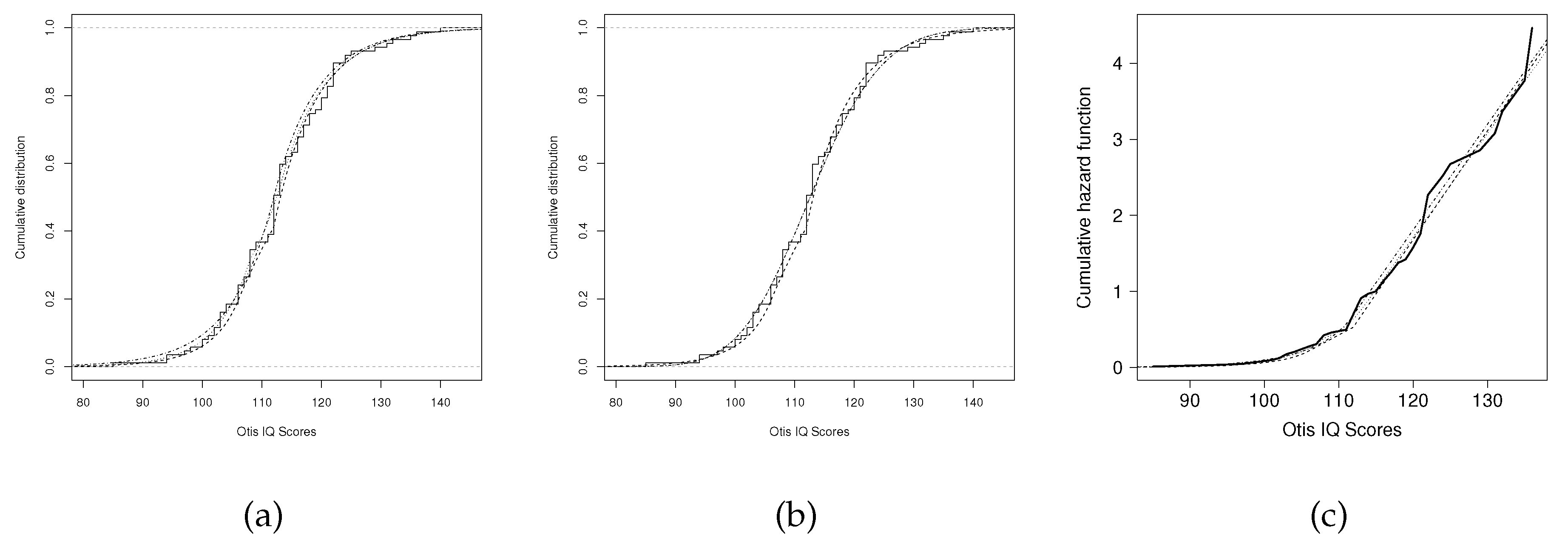

Table 1.
AIC, CAIC and HQIC criteria for the fitted models.
| Distribution | AIC | BIC | HQIC | |
|---|---|---|---|---|
| Laplace | 641.708 | 643.9977 | 643.6944 | |
| LS | 108.0222 | 641.6922 | 644.7422 | 646.6569 |
| SLPH | 111.9693 | 637.8516 | 641.2693 | 643.8092 |
| HNS | 99.9687 | 682.7748 | 685.2626 | 685.7536 |
| HNSHP | 99.9687 | 683.4016 | 686.1423 | 687.3734 |
| SN | 644.612 | 647.0998 | 647.5908 | |
| Gamma | 642.9468 | 645.2360 | 644.9327 | |
| Normal | 646.3490 | 648.6382 | 648.3349 | |
| MN | 646.4074 | 649.4574 | 651.3721 |
Table 2.
Estimation of the parameters, along with their standard errors, for the Laplace, LS, SLPH, HNS, and HNSHP models.
Table 2.
Estimation of the parameters, along with their standard errors, for the Laplace, LS, SLPH, HNS, and HNSHP models.
| Estimate | Laplace | LS | SLPH | HNS | HNSHP |
|---|---|---|---|---|---|
| 112.0004 | 110.6122 | 105.9556 | |||
| (0.0308) | (1.1075) | (0.4240) | |||
| 113.3408 | 111.9993 | ||||
| (0.9016) | (0.1693) | ||||
| 7.1859 | 5.6885 | 5.9306 | 1382.2189 | 272.5887 | |
| (0.7706) | (1.3427) | (1.1603) | (598.4787) | (108.9069) | |
| 7.3183 | 2.1697 | 6.2681 | 17.7197 | ||
| (1.0452) | (0.5466) | (2.5036) | (0.1300) | ||
| 0.3093 | 0.1867 | ||||
| (0.0638) | (0.0214) |
Table 3.
Estimation of the parameters, along with their standard errors, for the SN, Gamma, Normal, and MN models.
Table 3.
Estimation of the parameters, along with their standard errors, for the SN, Gamma, Normal, and MN models.
| Estimate | SN | Gamma | Normal | MN |
|---|---|---|---|---|
| 105.724 | 112.862 | 111.6556 | ||
| (3.119) | (1.028) | (2.1347) | ||
| 113.7674 | ||||
| (2.5908) | ||||
| 11.910 | 1.2396 | 9.589 | 35.9973 | |
| (2.076) | (0.1880) | (0.2349) | (42.1964) | |
| 130.2105 | ||||
| (81.5536) | ||||
| 1.143 | 139.9127 | 0.4278 | ||
| (0.684) | (21.1856) | (0.6189) |
Disclaimer/Publisher’s Note: The statements, opinions and data contained in all publications are solely those of the individual author(s) and contributor(s) and not of MDPI and/or the editor(s). MDPI and/or the editor(s) disclaim responsibility for any injury to people or property resulting from any ideas, methods, instructions or products referred to in the content. |
© 2025 by the authors. Licensee MDPI, Basel, Switzerland. This article is an open access article distributed under the terms and conditions of the Creative Commons Attribution (CC BY) license (http://creativecommons.org/licenses/by/4.0/).
Copyright: This open access article is published under a Creative Commons CC BY 4.0 license, which permit the free download, distribution, and reuse, provided that the author and preprint are cited in any reuse.


